Deep Reinforcement Learning-Based Two-Phase Hybrid Optimization for Scheduling Agile Earth Observation Satellites

Abstract

The multi-agile Earth observation satellite scheduling problem is challenging because of its large solution space and substantial task volume. This study generates observation schemes for static tasks over an execution period. To balance solution quality and computational efficiency, a deep reinforcement learning (DRL)-based algorithmic framework is proposed. A Markov decision process (MDP) is formulated as the foundational model for the DRL architecture. To mitigate problem complexity, the action space is decomposed into two interdependent decision layers: task sequencing and resource allocation. Given the resource occupation constraints during action execution, a novel reward function is designed by integrating resource occupation utility into the immediate reward mechanism. Corresponding to these dual decision layers, a Two-Phase Hybrid Optimization (TPHO) framework is developed. The task sequencing subproblem is addressed through an encoder–decoder architecture based on sequence-to-sequence learning. To preserve resource diversity throughout the scheduling horizon, a maximum residual capacity (MRC) heuristic is introduced. A comprehensive experimental suite is constructed, incorporating multi-satellite scheduling scenarios with capacity and temporal constraints. The experimental results demonstrate that the TPHO framework with MRC rules achieves superior performance, yielding a total reward improvement exceeding 16% compared with the A-ALNS algorithm in the most complex scenario involving 1200 tasks, yet requiring less than 3% of the computational duration of A-ALNS.

1. Introduction

Earth observation satellites (EOSs) provide large-scale observation coverage and are equipped with optical instruments to take photographs of specific areas at the request of users [1,2,3]. EOSs have been extensively employed in scientific research and application, mainly in environmental and disaster surveillance, ocean monitoring, agricultural harvesting, etc. [4]. Recently, agile EOSs (AEOSs) have drawn significant attention as a new generation of these platforms [5]. Unlike conventional EOSs, AEOSs possess three-axis (roll, pitch, and yaw) maneuverability, which amplifies flexibility and expands the solution space of their task scheduling. Cooperatively multiple AEOSs can serve various demands, such as multi-angular observation and wide area observation [6]. Consequently, multi-AEOS (MAEOS) scheduling has become a primary focus of satellite platforms.

However, although the number of AEOSs in orbit is increasing, they are still limited because of the vast number of applications they can be used for [7,8]. Therefore, an effective scheduling algorithm must be developed to improve the efficiency of observation systems. The MAEOS scheduling problem (MAEOSSP) is a large-scale combinatorial optimization problem and has been proven to be NP-hard [9]. Algorithms applied to MAEOSSP are usually classified as exact methods, heuristic methods, metaheuristic methods and machine learning methods [10].

Exact methods, such as mixed-integer linear programming [9], dynamic programming [11], and branch and price [12], provide optimal solutions and are limited to the scale and complexity of corresponding problems. Simple heuristic rules are extensively used in most optimization problems because they are efficient and intuitive [13,14,15]. Owing to their low computational complexity, heuristic methods have been widely applied in practical satellite scheduling, such as Pleiades in France [16], FireBIRD in Germany [17], and EO-1 in the USA [18]. Heuristic methods can speed up the process by finding a satisfactory solution, but studies and engineering projects have also indicated that heuristic results can be improved further. Metaheuristic methods typically provide satisfactory observation plans with a longer run time. Various metaheuristic algorithms have been proposed, including genetic algorithms and their variants [19,20,21,22], tabu search [23,24,25], simulated annealing [26], ant colonies and their variants [27], differential evolution algorithms [28], and large neighborhood search [29,30]. However, the search difficulty and solution times of these algorithms increase dramatically as the scale of the problem increases. Traditional exact and metaheuristic algorithms cannot meet the requirements of high efficiency and fast response in practical applications [31].

A major breakthrough in deep reinforcement learning (DRL) was achieved by Mnih et al. [32], where their proposed Deep Q-Network (DQN) demonstrated for the first time that DRL could attain human-level performance in complex decision-making tasks. In recent years, DRL has made remarkable achievements in games and has been applied to combinatorial optimization problems [33,34,35,36,37]. Combinatorial optimization allows one to optimally select variables in a discrete decision space, which is similar to the action selection of DRL. Moreover, with its “offline training and online decision making” characteristics, DRL demonstrates the potential for quick responses to requirements and shows a high solving speed compared with metaheuristics [38].

Therefore, DRL has become a promising method for solving satellite scheduling problems. Research efforts on DRL have been dedicated to single-AEOS scheduling [39,40,41,42], but there is little research on DRL for MAEOS scheduling.

Research efforts have been dedicated to addressing single-satellite Earth observation scheduling problems through DRL. Wang et al. [39] integrated case-based learning and a genetic algorithm to schedule EOS. Shi et al. [40] proposed an efficient and fair proximal policy optimization-based integrated scheduling method for multiple tasks using the Satech-01 satellite. Wang et al. [41] formulated a dynamic and stochastic knapsack model to describe the online EOS scheduling problem and proposed a DRL-based insertion process. He et al. [42] investigated a general Markov decision process (MDP) model and a Deep Q-Network for AEOS scheduling, and this solution method has also been employed for satellite range scheduling [43]. Chen et al. [44] regarded neural networks as feasible rule-based heuristics in their proposed end-to-end DRL framework. Zhao et al. [45] proposed a two-phase neural combinatorial optimization approach to address the EOS scheduling problem. Lam et al. [46] proposed a DRL-based approach that could provide solutions in nearly real time. Huang et al. [10] addressed the AEOS task scheduling problem within one orbit using the deep deterministic policy gradient (DDPG) method. Huang et al. [47] focused on decision-making in the task sequence and proposed a dynamic destroy deep-reinforcement learning (D3RL) model with two application modes. Liu et al. [48] proposed an attention decision network to optimize the task sequence in the AEOS scheduling problem. Liu et al. [49] presented a DRL algorithm with a local attention mechanism to investigate the single agile optical satellite scheduling problem. Wei et al. [50] introduced a DRL and parameter transfer based approach to solve a multi-objective agile earth observation satellite scheduling problem. Chun et al. [31] investigated a graph attention network-based decision neural network for the agile Earth observation satellite scheduling problem.

Compared with single-EOS scheduling, there is little research on DRL for MAEOS scheduling. Dalin et al. [51] proposed a DRL-based multi-satellite mission planning algorithm for high and low-orbit AEOSs, which kept the revenue rate difference compared with A-ALNS [30] below 5%. Wang et al. [52] focused on the autonomous mission planning problem for AEOSs, in which the visible time window (VTW) was set as a time interval. Li et al. [53] tackled the issue of multi-satellite rapid mission re-planning using a deep reinforcement learning method that incorporated mission sequence modeling. Chen et al. [54] addressed a multi-objective learning evolutionary algorithm for solving the multi-objective multi-satellite imaging mission planning problem. Wang et al. [55] developed an improved DRL method to address the MAEOSSP with variable imaging durations. Song et al. [56] introduced a genetic algorithm (GA) framework incorporating DRL for generating both initial solutions and neighborhood search solutions to address the multitype satellite observation scheduling problem. These studies focus on scenarios in which each task has only one VTW in each satellite.

In this study, we propose a DRL-based two-phase hybrid optimization (TPHO) method to generate an observation plan for the MAEOSSP. For each AEOS, tasks may have different numbers of VTWs. We propose an encoder–decoder network to optimize the task sequence and a heuristic method to allocate satellites for tasks. We model the MAEOS scheduling process using with a finite MDP with a continuous state space. The major contributions of this study are summarized as follows:

• An MDP for the MAEOSSP is constructed, in which the action space is decomposed into task action and resource action subspaces corresponding to the task sequence and resource allocation subproblems, and a new reward function is proposed.
• A DRL-based TPHO framework is proposed for the MAEOSSP. An encoder–decoder network in TPHO is designed to determine the task sequence, and a heuristic method is proposed to optimize the resource allocation problem.
• A comprehensive experiment is conducted to examine the performance of our method. Based on the computational results, the proposed method has proven to be effective and has high time efficiency. The experimental results also show that this study provides an intuitive and effective resource allocation rule in capacity limited application scenarios.

The remainder of this study is organized as follows: Section 2 presents the MAEOSSP in detail. Section 3 describes the proposed methods. Section 4 presents the experimental results, followed by discussions in Section 5. Section 6 presents the conclusions.

2. Problem Description

This study generates observation schemes for static tasks over an execution period. The tasks observe point targets according to user demands that include the latitude and longitude of the point target, observation duration, required observation time, etc. All user demands in the past period are collected and sent to the operation center. Then, considering the objectives and constraints, the operation center exports an observation scheme based on optimization algorithms. Subsequently, the scheme codes are sent to satellites, which execute tasks according to the uploaded scheme codes. After the current execution period ends, the observation system proceeds to the next execution period.

In practical management, generating a schedule can be considerably complicated because many details must be considered, such as regulations and user requirements. Following previous research [6,30,56,57], we simplified the problem by considering several assumptions.

(1)

A solar panel can provide sufficient energy for each satellite.

(2)

The download management of the acquired images is not considered because this issue falls outside the scope of this study.

(3)

There is, at most, one observation sensor running on a satellite at any time.

(4)

The maneuver time for pitch and roll maneuvers is considered when calculating the attitude transition time between two continuous tasks.

(5)

Observation tasks are point targets and targets preprocessed to be covered in a single observation.

(6)

Each task can be conducted once at most and does not need to be repeated.

(7)

If a task is successfully scheduled, it can be executed successfully without being affected by other factors.

(8)

The task and its execution demands are defined before scheduling starts; no new tasks or variations in demands occur.

Given the above assumptions, the MAEOSSP in this study can be described as follows. The task set containing a total of M tasks is defined as $I=\left\{\mathrm{1,2},\cdots , M\right\}$. For task $i\in I$, the observation time required by the user is $\left[{rs}_i,{re}_i\right]$, the observation duration is $d_i$, the observation profit is $P_i$, and the storage occupied by $i$ is $s_i$. The satellite set is $J=\left\{\mathrm{1,2},\cdots , N\right\}$. Each satellite, $j\in J$, has a memory capacity of $C_j$. The number of VTWs for task $i$ in satellite $j$ is $n_{twij}$. The set of VTWs for task $i$ in satellite $j$ is ${TW}_{ij}=\left\{{tw}_{ijk}|k=\mathrm{1,2},\cdots ,n_{twij}\right\}$, where ${tw}_{ijk}=\left[{tws}_{ijk,}{twe}_{ijk}\right]$. $\left[{ts}_{ij,}{te}_{ij}\right]$ represents the observation time for task $i$, where ${te}_{ij}={ts}_{ij}+d_i$.

The symbols and notations are shown in

Table 1. Symbols and notations.

Notations	Description	Notations	Description
$I$	Set of observation tasks	$A_t$	Set of task index
$J$	Set of involved AEOSs	$A_r$	Set of AEOS index
${TW}_{ij}$	Set of VTWs for task $i$ in AEOS $j$	$S_t$	Vector of task state at time step $t$
$n_{twij}$	Number of VTWs for task $i$ in AEOS $j$	$s_i^t$	Vector of state element of task $i$.
${tws}_{ijk}$	Start time of $k$th VTW for task $i$ in AEOS $j$	$x_i$	Vector of static state elements of task $i.$
${twe}_{ijk}$	End time of $k$th VTW for task $i$ in AEOS $j$	$d_i^t$	Vector of dynamic state elements of task $i$.
${rs}_i$	Start time of required OTW of task $i$	$X$	Matrix of static elements
${re}_i$	End time of required OTW of task $i$	$D_t$	Matrix of dynamic elements
${ts}_{ij,}$	Start time of observation for task $i$ in AEOS $j$	$P_i$	Observation profit of task $i$
${te}_{ij}$	End time of observation for task $i$ in AEOS $j$	${st}_i^t$	Storage occupied by task $i$.
θpij	Pitch attitude angle to task i by AEOS j	${rc}_i^t$	Remaining storage in all satellites for task $i$.
θrij	Roll attitude angle to task i by AEOS j,	$s_i$	Required storage of task $i$
vp	Angular velocity of the pitch maneuver	$C_j$	Memory capacity of AEOS $j$
vr	Angular velocity of the roll maneuver	$n_{twij}$	Number of VTWs for task $i$ on AEOS $j$
$d_i$	Observation duration of task $i$	${ftw}_i^t$	FTWs for task $i$ at time step $t.$
${ttw}_i^t$	Total length of FTWs in all satellites for task $i$ at time step $t$.	${eet}_i^t$	Earliest end time of task $i$ in all satellites at time step $t$
$x_{ij}$	If task $i$ is observed by AEOS $j$, and $x_{ij}=0$ otherwise.	$y_{ij\tau }$	If task $i$ is observed by AEOS $j$ and start time of task $i$ is $\mathsf{\tau }$, and $y_{ij\tau }=0$ otherwise.
${tr}_{mnj}$	Attitude transition time between two adjacent tasks $m$ and $n$	${sch}_i^t$	If task $i$ has been scheduled at time step $t$, ${sch}_i^t=1$, and ${sch}_i^t=0$, otherwise.

OTW—observation time window; FTW—feasible time window.

.

• Objective function:

The objective function of the MAEOSSP in this study is to maximize the total observation profit of all scheduled tasks. The objective function is defined as follows:

$$\mathrm{Maximize}: f={\displaystyle \sum _{j\in J}{\displaystyle \sum _{i\in I}{x}_{ij}{P}_i}},$$

(1)

where $x_{ij}=1$ if task $i$ is observed by satellite $j$, and $x_{ij}=0$ otherwise.

2.

Uniqueness constraint:

All tasks are one-time tasks. That is, each task can be observed no more than once over the entire time horizon.

$${\displaystyle \sum _{j=1}^N{\displaystyle \sum _{k=1}^{n_{twij}}{\displaystyle \sum _{\tau =tw{s}_{ijk}}^{tw{e}_{ijk}}{y}_{ij\tau }\tau }}}\le 1, i\in I,$$

(2)

where $y_{ij\tau }=1$ if task $i$ is observed by satellite $j$ and the start time of task $i$ is $\mathsf{\tau }$, and $y_{ij\tau }=0$ otherwise.

3.

Memory capacity constraint:

The total storage consumed by observed tasks for each satellite cannot exceed the memory capacity of the satellite.

$${\displaystyle \sum _{i\in I}{x}_{ij}{s}_i}\le C_j, j\in J,$$

(3)

4.

Observation time request constraint:

Task $i$ can be observed by any satellite, but the observation should start and be completed within the required observation time by users.

$$r{s}_i\le t{s}_i<t{e}_i\le r{e}_i, i\in I$$

(4)

5.

VTW constraint:

If task $i$ is observed by satellite $j$, the observation should start and be completed within VTW ${tw}_{ijk}$, where ${tw}_{ijk}\in {TW}_{ij}$.

$$tw{s}_{ijk}\le t{s}_i<t{e}_i\le tw{e}_{ijk}, i\in I, x_{ij}=1$$

(5)

6.

Attitude transition time constraint:

When two adjacent tasks, $i$ and $k$, are observed by satellite $j$, the time gap between the two tasks should not exceed the satellite attitude transition time, ${tr}_{ikj}$:

$$t{e}_i+t{r}_{ikj}\le t{s}_k,$$

(6)

where the transition time, ${tr}_{ikj}$, is the ratio of angles for observing the two tasks on satellite $j$ at the start time of the observation and the satellite maneuvering velocity.

The attitude transition time, ${tr}_{ikj}$, is calculated as follows:

$$t{r}_{ikj}=\max \left\{{\displaystyle \frac{\left|{\theta }_{pij}-{\theta }_{pkj}\right|}{v_p}},{\displaystyle \frac{\left|{\theta }_{rij}-{\theta }_{rkj}\right|}{v_r}}\right\},$$

(7)

where θ_pij is the pitch attitude angle to task i observed by satellite j, θ_rij is the roll attitude angle to task i observed by satellite j, and v_p and v_r are the angular velocities of the pitch and roll maneuvers, respectively.

Based on the assumptions, objective function, and constraints of the problem, we present a detailed solving method in Section 3.

3. Solving Method

The MAEOSSP investigated in this study involves determining the execution resources and time windows for each task under temporal and capacity constraints to optimize the objective function. Given the finite nature of satellite resources, tasks exhibit competitive relationships where scheduling sequences critically influence objective values. To mitigate complexity, the problem is decomposed into three interdependent decisions: task sequence determination, resource allocation, and execution time window determination. Once the task sequence is established, the subsequent focus narrows to identifying appropriate resources and temporal windows for individual tasks. As a promising approach, deep reinforcement learning (DRL) demonstrates balanced capabilities in decision quality and efficiency and has shown good sequential decision-making abilities, motivating our proposed DRL-based algorithm for task sequence determination.

DRL updates model parameters through agent–environment interactions, with the MDP framework serving as its foundational model, comprising states, actions, state transitions, and reward mechanisms. Establishing an MDP enables the precise specification of agent–environment interactions, which we systematically formalize in this section.

The state vector, representing environmental characteristics, is the input to the deep neural network. To enhance feature representation, state elements are categorized into static and dynamic elements based on their value variability during iterations.

Actions, the network’s output, constitute the agent’s decision space. While environmental state transitions must jointly determine task sequences, resource allocations, and temporal windows, the deep network primarily generates sequence decisions. This necessitates complementary mechanisms for resource and execution time determination. Considering computational efficiency, heuristic methods are employed. Given that tasks with visible time windows form satellite-specific sets, different satellites correspond to sets with different tasks due to distinct orbital parameters. To preserve resource diversity during the whole scheduling process, a maximum residual capacity (MRC) rule is proposed. An MRC rule indicates that a feasible satellite with maximum residual capacity is allocated to the determined task. This mechanism ensures that the observation system maintains resource diversity without premature depletion due to storage capacity constraints. Following previous studies [26,30,42,48], the beginning execution time of the determined task is set to the earliest of its feasible time windows in the determined satellite, i.e., the Earliest Start Time (EST) rule.

State transitions occur through the interplay of current states, DRL-generated task sequences, and heuristic-based resource allocations, with the agent receiving immediate reward feedback. The agent optimizes its policy by maximizing cumulative rewards representing long-term returns. Upon completing the scheduling process, the total return of the whole scheduling process is obtained. However, determining the contributions of individual step decisions to final returns remains challenging. As each decision schedules one task, task profit has naturally served as the immediate reward feedback in previous studies [42,47,48].

Nevertheless, task execution simultaneously consumes finite resources, significantly impacting long-term returns. In this study, resources are categorized into temporal resources and storage capacity resources. Temporal resources involve complex factors such as durations, visible time windows, and transition time, making them difficult to simply characterize. Furthermore, since task execution timing is determined by the EST (Earliest Start Time) heuristic, temporal attributes are partially accounted for in the scheduling process. Consequently, a reward function combining task profit and storage consumption ratios is proposed. This formulation incorporates the impacts of both resource consumption and task profit on cumulative returns. Given that the reward values undergo standardization prior to neural network training, the introduction of weighting coefficients to either task profit or storage consumption becomes unmeaningful. Section 3.1 describes the description of the Markov decision process model in detail.

Based on the above description, we propose a DRL-based TPHO framework. A deep neural network determines a task action, then based on the task action, a heuristic algorithm determines the resource action and the execution time. The decisions of the deep neural network and heuristic algorithms jointly drive the state transition of the environment. The sample (state, task action, reward, and next state) is generated in this process and trains the deep neural network model. Figure 1 shows the interaction between the environment, MDP model, and TPHO framework. The deep neural network in TPHO determines the task sequence. It receives task information sequences that describe the environment and outputs probability sequences for task selection. Since encoder–decoder architecture is a universal framework for sequence-to-sequence learning, an encoder–decoder is designed to determine the task action.

The state vector comprises both static and dynamic elements, where static components maintain invariant values across decision steps while dynamic counterparts vary temporally. Given their distinct characteristics, these elements undergo separate feature encoding through individual fully connected layers. This architectural design serves dual purposes: (1) the fully connected structure prevents information loss through linear transformation preservation, and (2) parallel encoding significantly reduces computational overhead compared with concatenation before encoding.

To provide scheduling sequences for the neural network, gated recurrent unit (GRU) networks receive historical static elements from previously scheduled tasks, effectively capturing sequential dependencies. GRU selection over long short-term memory (LSTM) networks is strategically motivated by two factors [58]: (1) the moderate sequence lengths in this decision-making context and (2) the limited dataset scale characteristic of satellite scheduling problems. The GRU’s streamlined architecture with fewer gating mechanisms enables accelerated training convergence while maintaining essential memory retention capabilities.

Section 3.2 details the encoder–decoder network and Section 3.2 details the training process. To train the encoder–decoder network, the soft actor–critic (SAC) algorithm is employed. According to Liu et al. [59], proximal policy optimization (PPO) faces stability challenges, and deep deterministic policy gradient (DDPG) and SAC demonstrate robust performance, notably in moderate-elasticity scenarios. The real-world application of the SAC model further affirmed its practical viability, marking a significant performance improvement [59].

3.1. Markov Decision Process Model

The Markov decision process presents the state space of the environment, the action space of the agent, the state transition function, and the reward function. the state describes the features of the environment, based on which the proposed encoder–decoder network selects a task action. According to the state transition function, the next state is reached based on the current state, task action, and resource action decision made by the heuristic algorithm. Then, a reward from the environment is received.

• State space

The state, $S_t$, is described by the following equations:

$$S_t=\left\{s_1^t,s_2^t,\cdot \cdot \cdot ,s_M^t\right\},$$

(8)

$$s_i^t=\left\{x_i,d_i^t\right\},$$

(9)

$$x_i=\left\{d_i,P_i\right\},$$

(10)

$$d_i^t=\left\{sc{h}_i^t,tt{w}_i^t,ee{t}_i^t,s{t}_i^t,r{c}_i^t\right\}.$$

(11)

$$r{c}_i^t={\displaystyle \sum _{j\in J}\left(C_j-{\displaystyle \sum _{i\in I}{x}_{ij}^t{s}_i}\right)}$$

(12)

where $s_i^t$ is the state element of task $i$, including static elements, $x_i$, and dynamic elements, $d_i^t$. The value of static elements is unchanged in the entire decision process, and the value of dynamic elements may vary in each new state. If task $i$ has been scheduled before, ${sch}_i^t=1$, and ${sch}_i^t=0$, otherwise.

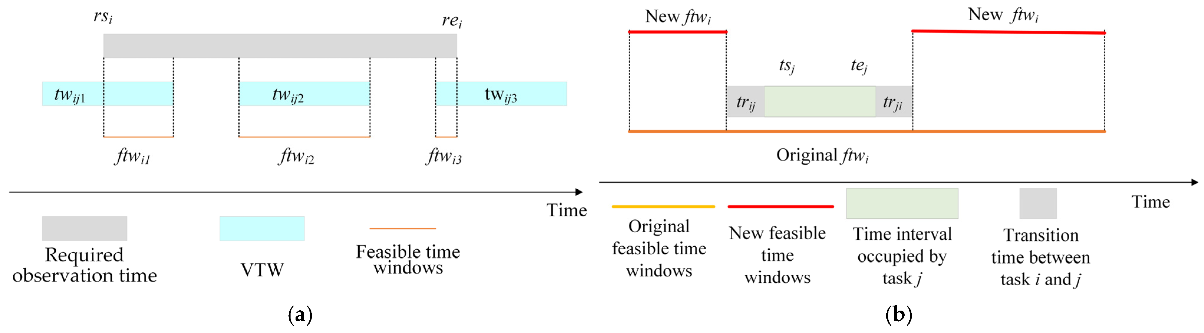
Following a previous study [48], we use two dynamic elements, ${ttw}_i^t$ and ${eet}_i^t$, to include the VTW information for each task. This state representation for the MDP can be applied to cases where tasks may have various numbers of VTWs.

${ttw}_i^t$ is the total length of the feasible time windows of all satellites for task $i$ at time step $t$. The feasible time windows for task $i$ at time step $t$, denoted as ${ftw}_i^t$, are the intersection of the required observation time by users and the VTWs for task $i$. Figure 2 describes the feasible time windows for task i.

${eet}_i^t$ is the earliest end time of task $i$ in all satellites at time step $t$. ${ftw}_i^t$ and ${eet}_i^t$ are updated at each time step, since a newly scheduled task may occupy the VTWs of task $i$. The value of each element is normalized by the maximum value.

${st}_i^t$ is the value of storage occupied by task $i$. ${rc}_i^t$ is the value of the remaining capacity in all satellites for task $i$. ${rc}_i^t$ is calculated by Equation (12). $x_{ij}^t=1$ if task $i$ is observed by satellite $j$ at time step $t$, and $x_{ij}^t=0$ otherwise. ${st}_i^t$ was originally a static element; here, ${st}_i^t$ and ${rc}_i^t$ are normalized together by the maximum value of the two types of elements. Thus, the value of ${st}_i^t$ may change over time steps.

• Action space

The action space is decomposed into the task action and resource action subspaces:

$$A=\left\{A_t,A_r\right\}$$

(13)

$$A_t=\left\{i|i=1,2,\cdot \cdot \cdot ,M\right\}$$

(14)

$$A_r=\left\{j|j=1,2,\cdot \cdot \cdot ,N\right\}$$

(15)

$A_t$ and $A_r$ are the collections of task number and satellite number, respectively. The action is selecting a task and a satellite, and the selected task is executed at the earliest of its feasible time windows by the selected satellite.

• State transition

If task $a$ and satellite $b$ are determined at time step $t$, the state, $S_t$, is then updated to $S_{t+1}$. In $S_{t+1}$, the static elements of all tasks remain unchanged. ${sch}_a^{t+1}$ is set to 0. The ${ttw}_i^{t+1}$ and ${eet}_i^{t+1}$ values of the other tasks are updated according to the time interval occupied by task $a$ in satellite $b$. The ${rc}_i^t$ for other tasks is updated according to the storage occupied by task $a$ in satellite $b$. The $s_i^t$ for all tasks is normalized by the updated maximum value.

• Reward function

In previous studies [42,47,48], the reward function is usually described as the increment in total profit. Here, we propose a novel reward function considering the storage occupied by the tasks, as defined in the following equation:

$$r_t=f\left(Y_t\right)-f\left(Y_{t-1}\right),$$

(16)

$$Y_t=\left\{y_{1t},y_{2t},\dots ,y_{Mt}\right\},$$

(17)

$$f\left(Y_t\right)={\displaystyle \sum _{i=1}^M\frac{P_i}{s_i}}{y}_{it},$$

(18)

where $y_{it}=\left\{\mathrm{0,1}\right\}$, $y_{it}=1$ if task $i$ has been scheduled at time step $t$, and $y_{it}=0$, otherwise. Normalizing of the reward function can avoid the impact of excessive or insufficient rewards on learning effectiveness and improve the comparability of reward values. Normalization of the reward function can avoid the impact of excessive or insufficient rewards on learning effectiveness and improve the comparability of reward values. Therefore, reward normalization is implemented to stabilize the learning dynamics during policy optimization. The value of $P_i/s_i$ is normalized by the maximum value of all tasks.

3.2. Two-Phase Hybrid Optimization

According to the MDP in this study, the decision process of the MAEOSSP is decomposed into a task sequence decision and a resource allocation decision. We propose a two-phase hybrid optimization that includes an encoder–decoder network for task sequence decision and a heuristic algorithm for resource allocation decision.

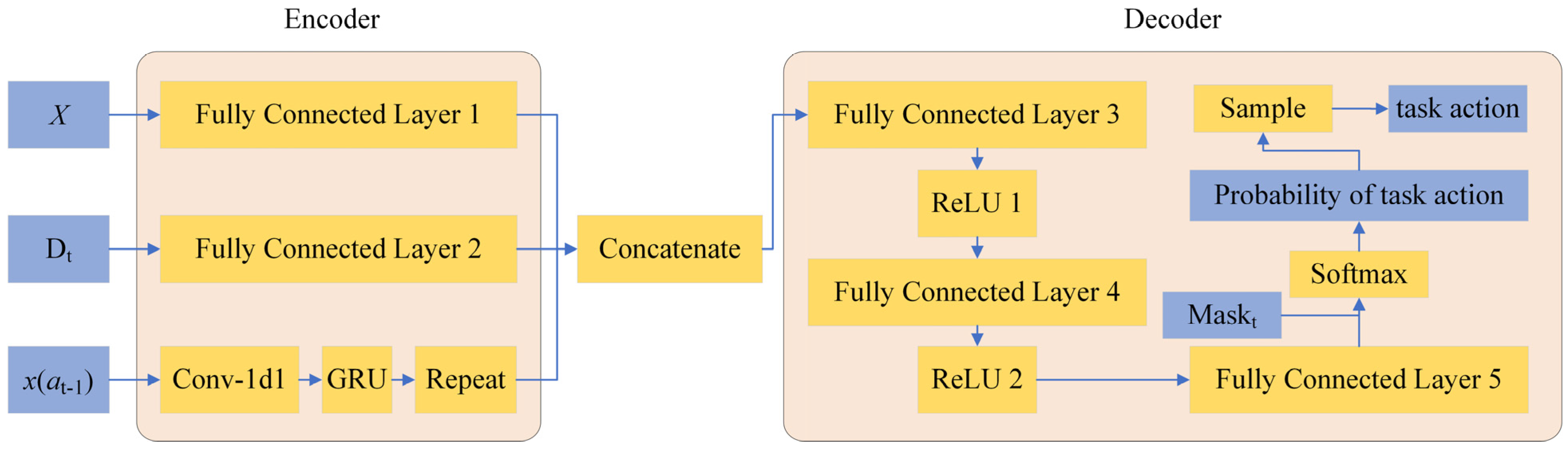
Since DRL has demonstrated a strong ability in sequential decision-making, we propose an encoder–decoder network to make decision in the task sequence. Figure 3 shows the architecture of the proposed encoder–decoder network. The encoder architecture comprises three parallel neural network layers, each specialized for encoding static elements, dynamic elements, and scheduling sequences. The decoder is structured as a stacked series of fully connected layers integrated with activation functions and incorporates the softmax-based normalization to probabilistically constrain the output space. Given their distinct characteristics, static and dynamic elements undergo separate feature encoding through individual fully connected layers. To provide scheduling sequences to the encoder–decoder network, the GRU receives historical static elements from previously scheduled tasks.

$X=transpose\left(\left[x_1, x_2,{\cdots ,x}_M\right]\right)$ is the matrix of the static elements, $D_t=transpose\left(\left[d_1^t, d_2^t,\cdots ,d_M^t\right]\right)$ is the matrix of the dynamic elements, $a_{t-1}$ is the task action selected in the last time step, $t-1$, and $x\left(a_{t-1}\right)$ is the $a_{t-1}$-th element in $X$. According to Equations (10) and (11), the dimension of $X$ is $\left(2,M\right)$, the dimension of $D_t$ is $\left(5,M\right)$, and the dimension of $x\left(a_{t-1}\right)$ is $\left(\mathrm{2,1}\right)$. $X$, $D_t$, and $x\left(a_{t-1}\right)$ are transposed before encoding, and after encoding, their dimensions are $\left(M,hd\right)$, $\left(M, hd\right)$, and $\left(1, hd\right)$, respectively. hd is the hidden dimensions of the fully connected layers and the GRU. We use a repeat operation to expand the dimension of encoded $x\left(a_{t-1}\right)$ from $\left(1, hd\right)$ to $\left(M, hd\right)$. Then, the encoded vectors are concatenated column-wise. In order not to lose information, $X$ and $D_t$ are encoded by fully connected networks. To save sequence information, $x\left(a_{t-1}\right)$ is encoded by a one-dimensional convolutional network and GRU.

The encoded inputs are concatenated as illustrated in Figure 3, after three linear layers and two activation layers, the value of each task action is obtained. The values are mapped to $\left(\mathrm{0,1}\right)$ by applying the Softmax function, and then the probability of each task action is obtained, based on which the task action selection is determined via sampling.

All neural network components, including fully connected layers, convolutional layers, GRUs, activation functions, and the Softmax layer are implemented using PyTorch 2.5.1. The specific implementation commands and corresponding parameters for each network layer are detailed in

Table A1. Specific implementation commands and corresponding parameters for each net-work layer.

Network Layer	PyTorch Implementation
Fully connected layer 1	torch.nn.Linear (2, hd)
Fully connected layer 2	torch.nn.Linear (5, hd)
Fully connected layer 3	torch.nn.Linear (3×hd, hd)
Fully connected layer 4	torch.nn.Linear (hd, hd)
Fully connected layer 5	torch.nn.Linear (hd, 1)
Fully connected layer 6	torch.nn.Linear (7, hd)
Fully connected layer 7	torch.nn.Linear (hd, hd)
Fully connected layer 8	torch.nn.Linear (hd, M)
Conv-1d1	torch.nn.Conv1d (2, out_channels = hd, kernel_size = 1, stride = 1)
GRU	torch.nn.GRU (hd, hd, 1, batch_first = True)
ReLU	torch.nn.functional.relu()
Softmax	torch.nn.functional.softmax()

in the Appendix A.

${Mask}_t$ is a mask matrix used to mask unfeasible task actions. ${Mask}_t=\left\{m_i|i=1,\dots ,M\right\}$, $m_i=1$ if task i is feasible at time step t and has not been scheduled, and $m_i=0$ otherwise. The probability of an unfeasible task is modified to zero by the mask matrix. Task i is feasible if least one satellite has feasible time windows for task i and the remaining capacity of the satellite is no less than the storage consumed by task i.

The task action is determined by the proposed encoder–decoder network, and then the resource action and beginning time decisions for task execution are needed to update the state. When allocating a satellite to observe the determined task, we consider decreasing the impact of resource occupation by the determined task on the feasibility of other unscheduled tasks. We propose a heuristic rule denoted as MRC that indicates a feasible satellite with maximum residual capacity is allocated to the determined task. The MRC rule is illustrated in Algorithm 1.

Algorithm 1 Heuristic rule MRC

Input: Determined task $a$, feasible time windows in satellite $j$ ${ftw}_a^j$, remaining capacity of satellite $j$ ${rc}^j$, initialize $rc$ = 0

Output: Number of the determined satellite $j_t$

1: for number of satellites $j$ = 1, 2, …, N do

2:    if ${ftw}_a^j=\varnothing$ do

3:       continue

4:    else if ${rc}^j>rc$ and ${rc}^j>s_i$ do

5:        $rc={rc}^j$

6:        $j_t=j$

7:     end if

8:  end for

In accordance with previous studies [26,30,42,48], the beginning execution time of the determined task is set to the earliest of its feasible time windows in the determined satellite. We also employ a heuristic rule as a comparison, denoted as EFT, indicating that a feasible satellite with the earliest feasible time windows is determined. The heuristic rule EFT is illustrated in Algorithm 2, where Max_v represents a big enough number, and $min\left\{{ftw}_a^j\right\}$ represents the earliest feasible time windows in satellite.

Algorithm 2 Heuristic rule EFT

Input: Determined task $a$, feasible time windows in satellite $j$ ${ftw}_a^j$, initialize $et$ = Max_v

Output: Number of the determined satellite $j_t$

1: for number of satellites $j$ = 1, 2, …, N do

2:    if ${ftw}_a^j=\varnothing$ do

3:        continue

4:    else if $min\left\{{ftw}_a^j\right\}<et$ and ${rc}^j>s_i$ do

5:        et $=min\left\{{ftw}_a^j\right\}$

6:        $j_t=j$

7:     end if

8:  end for

The task action and resource action, as determined by the encoder–decoder network and the heuristic rule, interact with the environment resulting in experience samples for training. The trained encoder–decoder network and heuristic rule form the proposed TPHO framework.

3.3. Training Process

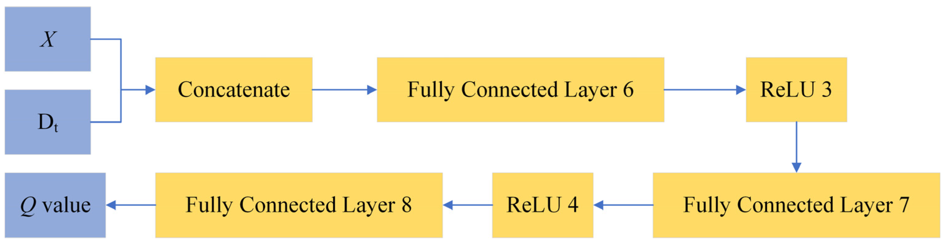
The SAC algorithm is employed to train the proposed encoder–decoder network [60]. SAC is an off-policy algorithm based on the actor–critic framework with maximum entropy. Figure 4 presents the architecture of the critic network in this study. The PyTorch 2.5.1 implementation specifications and corresponding parameters for each network layer are reported in Table A1 of the Appendix A.

The actor in the SAC algorithm maintains the diversity of exploration. A soft target update technique is used to smoothen the alterations during the training process. A dual Q-network is also adopted in SAC. The loss function of SAC is defined as follows [60]:

$$J_Q\left(\phi \right)=\mathrm{E}\left[{\left(Q\left(S_t,A^t\right)-r\left(S_t,A^t\right)-\gamma {\mathrm{E}}_{S_{t+1}}\left[{\mathrm{E}}_{{\pi }_{\theta }}\left[Q_{\tilde{\mathsf{\Phi }}}\left(S_{t+1},A^{t+1}\right)-\alpha \log {\pi }_{\theta }\left(A^{t+1}|S_{t+1}\right)\right]\right]\right)}^2\right],$$

(19)

$$J_{\pi }\left(\theta \right)={\mathrm{E}}_{s~D}\left[{\mathrm{E}}_{a~{\pi }_{\theta }}\left[\alpha \log {\pi }_{\theta }\left(a|s\right)-Q_{\phi }(s,a)\right]\right],$$

(20)

where $\phi$ represents the parameter of the $Q$ function, $Q_{\mathsf{\Phi }}\left(s,a\right)$ is the $Q$ function, $A^t$ is the action decision at time step $t$, $r$ is the reward value, $\tilde{\mathsf{\phi }}$ is the parameter of the target network, and $Q_{\tilde{\mathsf{\phi }}}$ is the target $Q$ value function.$\theta$ is the network parameter of the policy network ${\pi }_{\theta }$. $\alpha$ represents the regularization parameter of entropy. D is the experience replay pool used to store experience samples. The training process is illustrated in Algorithm 3, where Max_e is the maximum episode number. done = false indicates $S_{t+1}$ is not terminal. Learning begins when the number of samples in the experience pool reaches learning size.

Algorithm 3 Training process based on SAC

Input: Initial SAC parameters $\theta$, $\phi$, $\tilde{\phi }$, experience replay buffer D

Output: Trained encoder–decoder network

1: for number of episode = 1, 2, …, Maxe do

2:    Initial state $S_{t\leftarrow 0}$

3:    done = False

4:    while not done do

5:       Get a task action $a$ based on the network

6:       Get a resource action $a’$ based on the heuristic rule MRC

7:       Execute $a$ and $a’$, observe next state $S_{t+1}$

8:       Get reward r and update done

9:       Store experience sample ($S_t, a, r, S_{t+1}, done$) in D

10:        $S_t\leftarrow S_{t+1}$

11:       if size(D) > learning size do

12:          Sample a batch of ($S_t, a, r, S_{t+1}, d$) from D randomly

13:          Compute the loss as in (18)~(19)

14:          Update $\theta$, $\phi$, $\tilde{\phi }$ using Adam

15:        end if

16:     end for

3.4. Testing Process

The output of the encoder–decoder network is the probability distribution for the task action. During the training process, the task is selected according to the probability distribution. In the testing process, the action with the maximum probability is selected. Algorithm 4 describes the testing process.

Algorithm 4 Testing process

Input: Task profit $P_a$, trained encoder–decoder network, heuristic rule MRC, initialize $S_{t\leftarrow 0}$, done$\leftarrow$False, total profits$\leftarrow$0

Output: Total profits, observation plan

1: while not done do

2:    Input $S_t$ and sequence information into encoder–decoder network

3:    Select the task with the maximum probability

4:    Select a satellite based on MRC

5:    Execute $a$ at the earliest feasible time windows

6:    update done and state $S_t\leftarrow S_{t+1}$

7:    total profits = total profits + $P_a$

The performance of the proposed method is validated through numerical experiments in Section 4.

4. Results

A series of MAEOSSPs with different parameters were generated to evaluate our methods. Several advanced methods were employed as comparisons to verify the effectiveness of the proposed methods. All algorithms were implemented on a Dell Precision 3680 computer with an Intel Core i9-14900K @ 3.20 GHz, 32 MB RAM, with 27.8 GB video memory for NVIDIA Ge-Force RTX 3060 GPU and coded using Python 3.9. Algorithms based on learning were coded in PyTorch 2.5.1. The main parts of the computer are assembled in Xiamen and Kunshan, China.

4.1. Design of Experiments

The scheduling horizon was from 2022/09/01 00:00 to 2022/09/01 24:00. As shown in

Table 2. Simulation scenarios.

Region	Number of AEOSs	Number of Tasks	Training Scenarios	Test Scenarios
114–124°E, 30–45°N	2,3,4	300, 600, 900, 1200	12	60

, all scenarios were tested using two, three, and four AEOSs. The number of tasks changed from 300 to 1200 in increments of 300. Tasks were defined by the area corresponding to 114−124°E and 30−45°N and were distributed mainly in China. One training scenario and five test scenarios were used for each scale of task or satellite. In the following sections, X-Y represents scenarios in which the number of AEOSs is X and the number of tasks is Y.

The storage consumption and observation duration for each task were randomly generated between [1.6 GB and 3.3 GB] and [15 s and 30 s], respectively. To standardize the description of profit, the tasks were discretized into nine levels. Here, we randomly assigned an integer in a range of 1–9 to each task as the profit value. The VTWs of the AEOSs for tasks were obtained from the System Tool Kit (STK). AEOS coverage analysis was performed using the STK, with the GAOFEN constellation simulated to compute accessible time windows for target tasks. The angular velocities of the satellite pitch maneuver v_p and roll maneuver, v_r, were both set to 5°/s, and the orbit parameters of the AEOSs are listed in

Table 3. Orbit parameters.

Semi-Major Axis (km)	Orbital Inclination (°)	Right Ascension of the Ascending Node (°)	Orbital Eccentricity	Argument of Perigee (°)	Mean Anomaly (°)
7005	97.81	196.3165	0.0006736	208.4552	96.52
7129	98.41	129.9734	0.0001996	89.5171	188.83
7078	98.23	59.8261	0.0002885	111.2301	236.73
7019	97.96	202.6863	0.0010966	93.4251	279.04

.

Hyperparameter tuning in DRL algorithms lacks fixed rules. We referenced approximate parameter ranges from the existing literature [59,60] and finalized the parameters through pre-experiments.

Table 4. Training parameters.

Parameters	Value
Maximum number of episodes	50
Memory capacity	500
Learning size	200
Batch size	64
Discount factor	0.9
Learning rate of actor	1 × 10−4
Learning rate of critic	1 × 10−3
Regularization parameter of entropy	1 × 10−2
Soft update factor	0.005
Hidden dimension	256

lists the parameters of the proposed encoder–decoder network using in the training process. The parameter values were determined based on a pre-experiment implemented on scenarios with 2 AEOSs and 600 tasks (denoted as 2-600), in which the network with different values for each parameter was trained. The testing results are shown in Figure 5.

The median of the running time results is denoted as t*, and the median of the total profit results is denoted as TP*. In Figure 5, the area formed by values smaller than t* and greater than TP* is marked with a green shadow, representing the relatively balanced good results of the two indicators. Figure 5 shows that the result for the parameters with the values in Table 4 demonstrates a balance between total profit and temporal efficiency and obtains a higher total profit.

4.2. Training Analysis of the Proposed TPHO

As shown in

Table 5. Algorithm structures.

Algorithm	Group	Heuristic Rule	Reward Function	Network
TPHO-MRC	Our method	MRC	Equations (15)–(17)	Encoder–decoder
TPHO-EFT	Comparison	EFT	Equations (15)–(17)	Encoder–decoder
TPHO-Profit	Comparison	MRC	Increment in total profit	Encoder–decoder
TPHO-Linear	Comparison	MRC	Equations (15)–(17)	Linear

, three TPHO-based algorithms are compared to verify the performance of the specific designs for the proposed TPHO. TPHO-MRC is the proposed method, in which the reward function is defined as Equations (16)–(18), a proposed encoder–decoder network is used to generate the task sequence, and the MRC rule is used to allocate the satellite. In TPHO-EFT, the heuristic rule MRC is replaced by EFT. TPHO-Profit defines the increment in total profit as the reward function. TPHO-Linear employs multiple layers of fully connected networks to make decisions in the task sequence.

Figure 6 shows the total profit during the training process of the four algorithms in 12 training scenarios with different numbers of AEOSs and tasks. The total profit increases in the early stage and finally oscillates around a certain value, demonstrating that the network can learn to improve its policy and converge to a stable policy. The slope of the training curve indicates the learning efficiency of the network, and the height of the training curve shows the quality of the policy. Notably, in the 3-300 (Figure 6e) and 4-300 (Figure 6i) scenarios, the optimal solutions can be achieved using the initial strategies of the four methods.

Figure 6 shows that TPHO-MRC provides the best solution among the four algorithms after training and shows good learning efficiency in all training scenarios. The training curves also indicate that the total profit of TPHO-Profit converges to a lower value. Using EFT as the resource allocation rule, TPHO-EFT performs worse than other algorithms in scenarios with four AEOSs. TPHO-Linear obtains worse results than TPHO-MRC in scenarios 3-1200, 4-900, and 4-1200. This proves that the proposed encoder–decoder network, MRC rule, and designed reward function can improve the optimization performance of TPHO.

4.3. Testing Results

To evaluate the generalization ability of the four algorithms, we applied the trained TPHO-MRC, TPHO-Linear, TPHO-Profit, and TPHO-EFT algorithms to 60 test scenarios. We also compared the proposed algorithms with two existing metaheuristic algorithms: SA [26] and A-ALNS [30]. The average results for total profit (TP), standard deviation (SD), and coefficient of variation (CV) for five test scenarios for each satellite task size are listed in

Table 6. Comparison of testing results.

Number of AEOSs and Tasks	Value	TPHO-MRC	TPHO-Linear	TPHO-Profit	TPHO-EFT	A-ALNS	SA
2-300	TP	1425.2	1424.8	1423.6	1425.4	1360.2	1336.2
	SD	38.98	38.74	39.46	38.28	40.79	56.33
	CV	2.73%	2.72%	2.77%	2.69%	3.00%	4.22%
2-600	TP	2056	2055.2	1907	2047	1794.8	1749.8
	SD	36.34	35.29	39.40	37.01	27.60	85.67
	CV	1.77%	1.72%	2.07%	1.81%	1.54%	4.90%
2-900	TP	2313.8	2308.4	2277.2	2313.2	1949.4	1895.8
	SD	24.60	24.38	29.50	24.54	25.60	50.14
	CV	1.06%	1.06%	1.30%	1.06%	1.31%	2.64%
2-1200	TP	2467.4	2461.4	2152	2458.4	2011.4	1939.4
	SD	49.73	35.50	20.12	40.99	25.35	82.40
	CV	2.02%	1.44%	0.94%	1.67%	1.26%	4.25%
3-300	TP	1428	1428	1428	1428	1426.6	1417
	SD	37.50	37.50	37.50	37.50	38.87	31.53
	CV	2.63%	2.63%	2.63%	2.63%	2.72%	2.22%
3-600	TP	2583.2	2582.2	2579.8	2581.8	2347.2	2084.6
	SD	46.96	45.98	48.28	46.56	39.90	56.61
	CV	1.82%	1.78%	1.87%	1.80%	1.70%	2.72%
3-900	TP	3094.2	3093	2976	3092	2646	2429.8
	SD	32.74	33.34	47.83	32.09	60.55	66.16
	CV	1.06%	1.08%	1.61%	1.04%	2.29%	2.72%
3-1200	TP	3373.2	3121.4	3328.8	3370	2718	2419.6
	SD	46.84	46.13	41.77	46.53	123.09	202.53
	CV	1.39%	1.48%	1.25%	1.38%	4.53%	8.37%
4-300	TP	1428	1428	1428	1428	1428	1424.6
	SD	37.50	37.50	37.50	37.50	37.50	41.16
	CV	2.63%	2.63%	2.63%	2.63%	2.63%	2.89%
4-600	TP	2812	2811.4	2810	2758.8	2632.8	2212.6
	SD	63.67	63.88	62.49	60.21	52.73	174.35
	CV	2.26%	2.27%	2.22%	2.18%	2.00%	7.88%
4-900	TP	3688.6	3685.4	3674.2	3654	3244	2642.2
	SD	37.98	36.78	38.54	34.06	24.15	62.21
	CV	1.03%	1.00%	1.05%	0.93%	0.74%	2.35%
4-1200	TP	4126.8	4123.6	4101.8	4099.6	3482.8	2585.6
	SD	59.15	58.33	57.22	62.12	165.48	180.08
	CV	1.43%	1.41%	1.40%	1.52%	4.75%	6.96%

TP represents the total profit, SD represents the standard deviation, and CV represents the coefficient of variation.

, and the results are intuitively presented in Figure 7. Table 6 and Figure 7 show that TPHO-MRC obtains the highest total profit in all test scenarios, and the CV values of the TPHO-based algorithms are lower than 3%, demonstrating the stability of the algorithms. TPHO-MRC demonstrates a performance improvement exceeding 16% compared with the A-ALNS algorithm in scenarios involving 1200 observation tasks. A two-tailed Wilcoxon signed-rank test [61] was performed to pair six algorithms to ascertain the significance of the results. Notably, the results of the 3-300 and 4-300 scenarios are not included because most algorithms obtain the optimal solutions.

Table 7. Results of significance test.

Algorithm	TPHO-Linear	TPHO-EFT	TPHO-Profit	A-ALNS	SA
TPHO-MRC	0.001	0.002	0.001	0.001	0.001
TPHO-Linear		0.161	0.032	0.001	0.001
TPHO-EFT			0.097	0.001	0.001
TPHO-Profit				0.001	0.001
A-ALNS					0.001

details the significant test results. The results indicate that TPHO-MRC significantly outperforms other algorithms at the 1% level of significance, and algorithms based on TPHO significantly outperform the two metaheuristic algorithms, demonstrating the effectiveness of the proposed TPHO.

The average results for the runtimes of the six algorithms are listed in

Table 8. Testing runtimes.

Number of AEOSs and Tasks	Runtime(s)
	TPHO-MRC	TPHO-Linear	TPHO-Profit	TPHO-EFT	A-ALNS	SA
2-300	3.099	2.798	2.930	4.136	92.514	9.369
2-600	10.907	10.022	11.217	10.116	174.249	35.997
2-900	21.876	20.664	20.122	19.019	252.129	78.477
2-1200	35.800	34.665	29.784	30.826	1514.861	142.777
3-300	5.741	4.456	5.805	5.726	24.709	12.303
3-600	17.058	15.171	16.965	14.994	276.333	46.696
3-900	32.482	31.029	27.686	28.140	390.706	106.019
3-1200	54.714	52.903	46.446	45.561	2587.387	189.259
4-300	6.540	5.429	6.520	6.382	0.193	12.666
4-600	21.270	19.693	21.954	18.828	370.466	52.161
4-900	43.123	40.969	36.348	36.058	515.719	120.106
4-1200	70.073	69.514	69.203	58.393	3391.777	210.437

. Algorithms based on TPHO show better time efficiency than metaheuristic algorithms. The runtimes of the four TPHO-based algorithms are similar. TPHO-MRC could complete scheduling within 71 s for scenarios with up to 4 AEOSs and 1200 tasks, constituting less than 3% of the computational duration required by the A-ALNS algorithm. Figure 8 illustrates the runtime trends. As shown in Figure 8, the runtime of A-ALNS increases sharply as the number of AEOSs and tasks increases. The average runtime of A-ALNS for the 4-300 scenarios is 0.193, because all feasible tasks have been scheduled in the initial solution of the algorithm so that the algorithm terminates after generating the initial solution. By contrast, the runtimes of the TPHO-based algorithms increase slightly as the number of AEOSs and tasks increases. This indicates that the TPHO-based algorithms can efficiently complete scheduling for larger-scale MAEOSSPs.

4.4. Sensitivity Analysis

• Impact of the number of AEOSs and tasks

Figure 9 shows the average total profit and profit acquisition rate of TPHO-MRC under different numbers of tasks and AEOSs. The profit acquisition rate is the ratio of the total profit of scheduled tasks to the total profit of all tasks, reflecting the degree of task overload. Figure 9a shows that the total profit of TPHO-MRC increases with an increasing number of AEOSs and tasks. In the 3-300 and 4-300 scenarios, the profit acquisition rates are equal to 1, implying that all tasks are scheduled. As the number of tasks increases, the total profit increases, and the profit acquisition rate decreases. This is because excessive tasks exceed the resource ability of the AEOSs, but the TPHO-MRC can make good selection decisions from excess tasks to improve the total profit.

2.

Impact of satellite memory capacity

In the proposed TPHO-MRC, the designed reward function and heuristic rule are related to the memory capacity constraint. To evaluate the performance of algorithms under looser memory capacity constraints, we compared TPHO-MRC with TPHO-Profit and TPHO-EFT in scenarios in which the memory capacities of the AEOSs are set to 450 GB (increased by 100).

Table 9. Test results for scenarios with memory capacity = 450 GB.

Number of AEOSs and Tasks	TPHO-MRC		TPHO-Profit		TPHO-EFT
	Total Profit	Profit Acquisition Rate	Total Profit	Profit Acquisition Rate	Total Profit	Profit Acquisition Rate
2-300	1428	1.000	1428	1.000	1428	1.000
2-600	2386.8	0.846	2279.8	0.810	2368.8	0.841
2-900	2773.8	0.652	2751	0.647	2769	0.651
2-1200	2996.8	0.576	2719	0.523	2980.2	0.573
3-300	1428	1.000	1428	1.000	1428	1.000
3-600	2793.2	0.992	2790.2	0.991	2770.8	0.984
3-900	3614.4	0.860	3545.2	0.844	3599	0.857
3-1200	4022.4	0.714	4004.4	0.711	4015.6	0.713
4-300	1428	1.000	1428	1.000	1428	1.000
4-600	2817	1.000	2817	1.000	2802.2	0.995
4-900	4116.2	0.962	4110.4	0.961	3954	0.923
4-1200	4780.4	0.845	4773.6	0.843	4613.2	0.815

shows the detailed average total profit and profit acquisition rate for the three algorithms and that TPHO-MRC still obtains the best results among them. A significant test was also performed for the pairs of the three algorithms. TPHO-MRC significantly outperforms TPHO-Profit (p = 0.003) and TPHO-EFT (p = 0.003) in scenarios with relaxed memory capacity constraints.

The total profit increases with a rise in memory capacity. Figure 10 shows the rate of increase in total profit for the three algorithms. The rise in total profit increases as the task number increases and decreases as the AEOS number increases, aligning with the normal relationship between task load and capacity demand. The TPHO-Profit result increases the most and that of TPHO-EFT increases the least, except in 4-600 scenarios in which all tasks are executed by TPHO-Profit and TPHO-MTC. Notably, TPHO-EFT outperforms TPHO-Profit in 2-AEOS and 3-AEOS scenarios, but the opposite conclusion can be drawn in 4-AEOS scenarios, as shown in Table 6 and Table 9. This indicates that the MRC rule shows more prominent effectiveness in scenarios with more AEOSs.

The methods and experimental conclusions are discussed further in Section 5.

5. Discussion

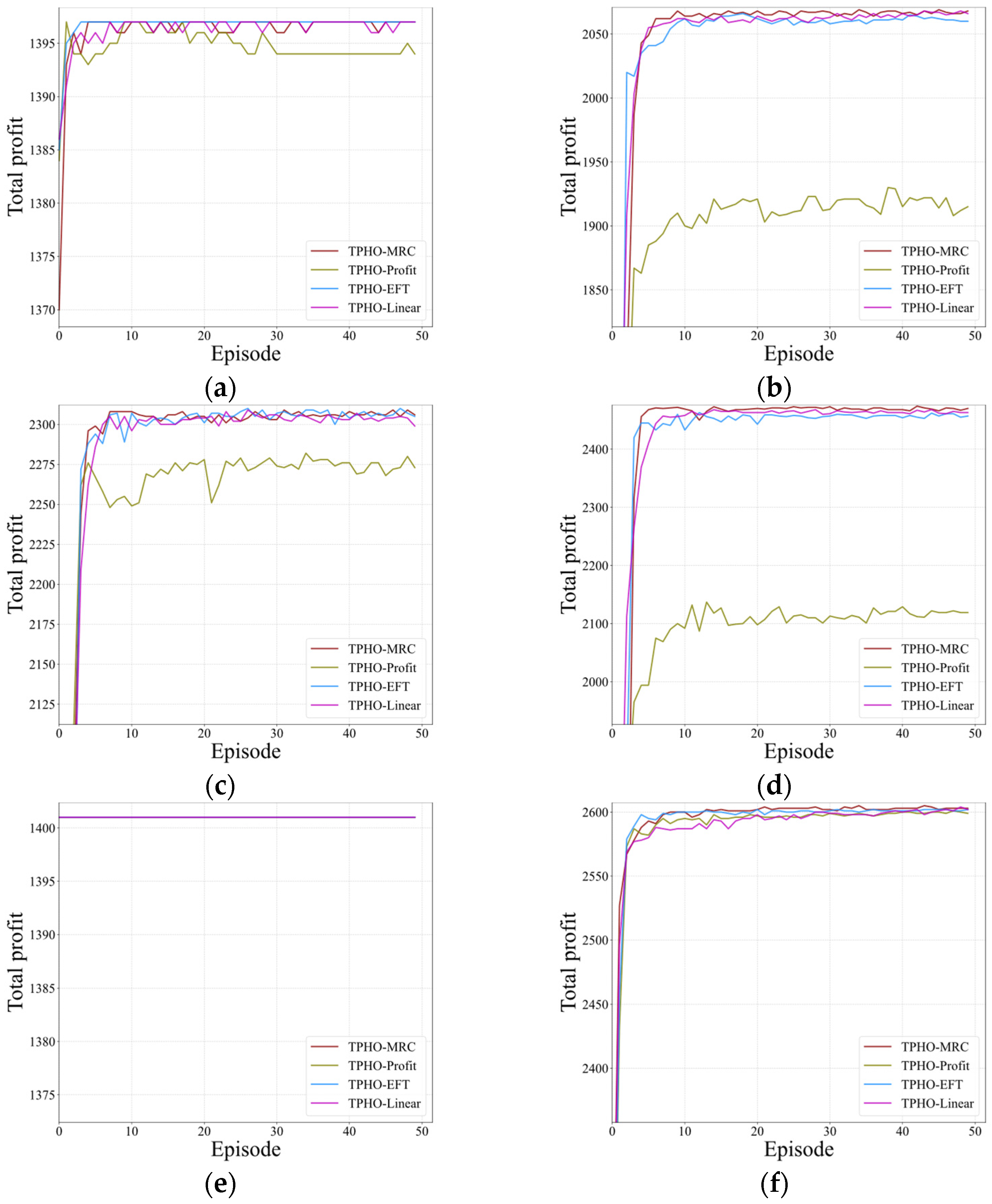
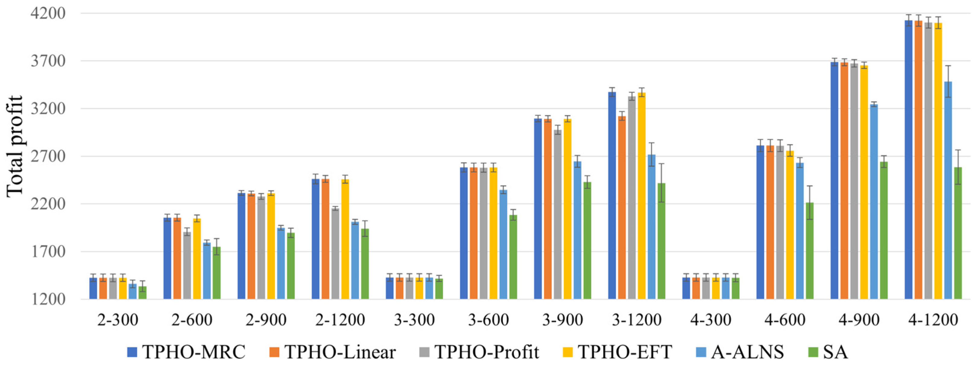
With the development of space science and technology, the collaborative operation of multiple AEOSs has shown advantages in enhanced remote sensing services, including speed. An effective scheduling algorithm is the key to improving the efficiency of AEOS applications. This study proposed a DRL-based TPHO framework with an effective heuristic rule, MRC, to rapidly generate an observation plan for the MAEOSSP. During the training process, the total profit increases at the beginning and then oscillates around a specific value, demonstrating that the network can converge on a stable policy. After training, the proposed method can be generalized to various application scenarios. According to the testing results, the proposed TPHO-MRC algorithm significantly outperforms other algorithms. Comparison results also indicate that the TPHO-based algorithms show good time efficiency and have the potential to apply to larger-scale MAEOSSPs.

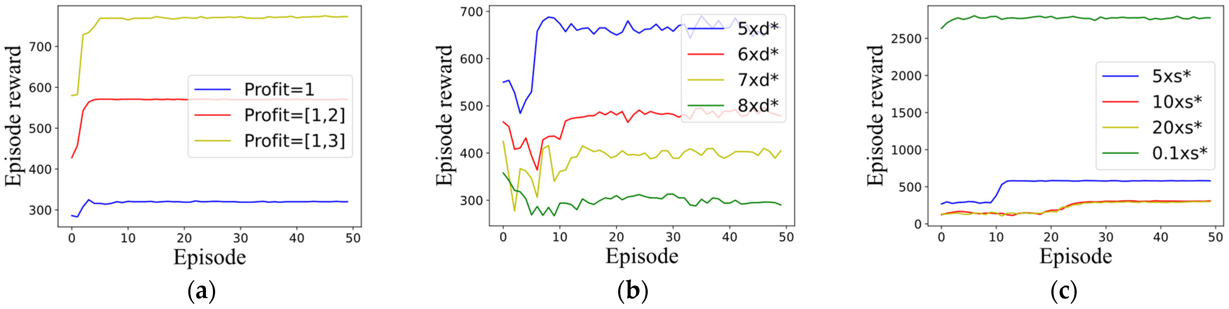
To further discuss the performance of the proposed TPHO-MRC, boundary value analysis of algorithm applicability was conducted. In the experimental section of this study, tasks were divided into nine priority levels based on importance, i.e., the task profit range was [1, 9]. Task reward serves as crucial information for the proposed algorithm’s task sequence decision-making. Here, we analyze the training convergence when differences in task importance decrease. Figure 11a shows the training curves when task profits are in ranges [1, 3], [1, 2], and all equal to 1. When there are only two profit levels, the algorithm can still converge near the maximum value of the training curve. When all profits are equal, although the algorithm converges, it fails to approach the maximum value, indicating that the current algorithm is more suitable for scenarios with distinct task priorities.

In our experiments, task observation durations ranged from d* = [15 s, 30 s]. We analyze the training convergence when extending observation durations. Figure 11b displays training curves for 5×, 6×, 7× and 8× original durations. The algorithm converges to maximum values at 5× and 6× duration, converges near initial values at 7×, and completely fails at 8× duration, demonstrating current applicability for observation durations within [90 s, 180 s].

For storage requirements, tasks occupied s* = [1.6 GB, 3.3 GB] with satellite capacity of 350 GB. Figure 11c shows training curves when storage demands increase to 5×, 10×, 20× and capacity reduces to 1/10. The algorithm maintains convergence to maximum values in both scenarios, indicating broad adaptability to storage requirement variations.

MAEOS scheduling usually serves as an oversubscription scenario in which the task load exceeds the resource ability. The proposed TPHO-MRC has shown the ability to make good selections from excess tasks. We also compared TPHO-MRC and TPHO-Profit with TPHO-EFT in two different memory capacity scenarios. The comparison results demonstrate that the proposed MRC rule is an intuitive and effective resource allocation rule in capacity-limited application scenarios.

6. Conclusions

This study investigates the MAEOS scheduling problem, described by an MDP model. In the MDP, the characteristics of the learning environment were presented by static and dynamic elements of the state. The action space was decomposed into two subspaces corresponding to the task sequence and resource allocation subproblems, and a new reward function was designed. Based on the MDP, we proposed a TPHO framework. An encoder–decoder network was designed to determine the task scheduling sequence, and a heuristic rule, MRC, was employed to allocate the resource. Comprehensive experiments were conducted to examine the performance of the TPHO framework. The results indicated that the proposed encoder–decoder network could converge on a stable policy. The proposed TPHO framework with the MRC rule significantly outperforms other algorithms, including two advanced algorithms (A-ALNS and SA). The computational results also showed that the TPHO-based algorithms showed high time efficiency for the MAEOSSP.

Owing to the considerable time efficiency and good generalization ability, the TPHO-MRC integrated with the target decomposition technique can be applied to MAEOSSP for area targets and mobile targets. Another promising direction involves using the proposed methods to address online scheduling or reactive scheduling. The proposed TPHO framework is a DRL-based general framework whose training stability and generalization ability are limited to the environment. Thus, it may not be suitable for more complex situations.

References

1. Balsamo, G.; Agustì-Parareda, A.; Albergel, C.; Arduini, G.; Beljaars, A.; Bidlot, J.; Blyth, E.; Bousserez, N.; Boussetta, S.; Brown, A. Satellite and in situ observations for advancing global Earth surface modelling: A review. Remote Sens. 2018, 10, 2038. [Google Scholar] [CrossRef]
2. Ban, Y.; Gong, P.; Giri, C. Global land cover mapping using Earth observation satellite data: Recent progresses and challenges. ISPRS J. Photogramm. Remote Sens. 2015, 103, 1–6. [Google Scholar] [CrossRef]
3. Zhao, Q.; Yu, L.; Du, Z.; Peng, D.; Hao, P.; Zhang, Y.; Gong, P. An overview of the applications of earth observation satellite data: Impacts and future trends. Remote Sens. 2022, 14, 1863. [Google Scholar] [CrossRef]
4. Gu, X.; Tong, X. Overview of China earth observation satellite programs [space agencies]. IEEE Signal Process. Mag. 2015, 3, 113–129. [Google Scholar]
5. Wang, X.; Wu, G.; Xing, L.; Pedrycz, W. Agile Earth Observation Satellite Scheduling over 20 Years: Formulations, Methods, and Future Directions. IEEE Syst. J. 2021, 15, 3881–3892. [Google Scholar] [CrossRef]
6. Xu, Y.; Liu, X.; He, R.; Chen, Y. Multi-satellite scheduling framework and algorithm for very large area observation. Acta Astronaut. 2020, 167, 93–107. [Google Scholar] [CrossRef]
7. Denis, G.; Claverie, A.; Pasco, X.; Darnis, J.-P.; de Maupeou, B.; Lafaye, M.; Morel, E. Towards disruptions in Earth observation? New Earth Observation systems and markets evolution: Possible scenarios and impacts. Acta Astronaut. 2017, 137, 415–433. [Google Scholar] [CrossRef]
8. Ustin, S.L.; Middleton, E.M. Current and near-term advances in Earth observation for ecological applications. Ecol. Process. 2021, 10, 1. [Google Scholar] [CrossRef]
9. Wang, J.; Demeulemeester, E.; Qiu, D. A pure proactive scheduling algorithm for multiple earth observation satellites under uncertainties of clouds. Comput. Oper. Res. 2016, 74, 1–13. [Google Scholar] [CrossRef]
10. Huang, Y.; Mu, Z.; Wu, S.; Cui, B.; Duan, Y. Revising the Observation Satellite Scheduling Problem Based on Deep Reinforcement Learning. Remote Sens. 2021, 13, 2377. [Google Scholar] [CrossRef]
11. Wang, J.; Song, G.; Liang, Z.; Demeulemeester, E.; Hu, X.; Liu, J. Unrelated parallel machine scheduling with multiple time windows: An application to earth observation satellite scheduling. Comput. Oper. Res. 2023, 149, 106010. [Google Scholar] [CrossRef]
12. Peng, G.; Song, G.; Xing, L.; Gunawan, A.; Vansteenwegen, P. An exact algorithm for agile earth observation satellite scheduling with time-dependent profits. Comput. Oper. Res. 2020, 120, 104946. [Google Scholar] [CrossRef]
13. Wang, P.; Reinelt, G.; Gao, P.; Tan, Y. A model, a heuristic and a decision support system to solve the scheduling problem of an earth observing satellite constellation. Comput. Ind. Eng. 2011, 61, 322–335. [Google Scholar] [CrossRef]
14. Chen, X.; Reinelt, G.; Dai, G.; Wang, M. Priority-Based and Conflict-Avoidance Heuristics for Multi-Satellite Scheduling. Appl. Soft. Comput. 2018, 69, 177–191. [Google Scholar] [CrossRef]
15. Chang, Z.; Chen, Y.; Yang, W.; Zhou, Z. Mission planning problem for optical video satellite imaging with variable image duration: A greedy algorithm based on heuristic knowledge. Adv. Space. Res. 2020, 66, 2597–2609. [Google Scholar] [CrossRef]
16. Beaumet, G.; Verfaillie, G.; Charmeau, M.C. Feasibility of autonomous decision making on board an agile earth-observing satellite. Comput. Intell. 2011, 27, 123–139. [Google Scholar] [CrossRef]
17. Wille, B.; Wörle, M.T.; Lenzen, C. VAMOS–verifification of autonomous mission planning on-board a spacecraft. IFAC Proc. 2013, 46, 382–387. [Google Scholar] [CrossRef]
18. Chien, S.; Tran, D.; Rabideau, G.; Schaffer, S.; Mandl, D.; Frye, S. Planning operations of the earth observing satellite EO-1: Representing and reasoning with spacecraft operations constraints. In Proceedings of the 6th International Workshop on Planning and Scheduling for Space (IWPSS), Pasadena, CA, USA, 19–21 July 2009. [Google Scholar]
19. Fatos, X.; Sun, J.; Barolli, A.; Biberaj, A.; Barolli, L. Genetic algorithms for satellite scheduling problems. Mob. Inf. Syst. 2012, 8, 351–377. [Google Scholar]
20. Zhibo, E.; Shi, R.; Gan, L.; Baoyin, H.; Li, J. Multi-satellites imaging scheduling using individual reconfiguration-based integer coding genetic algorithm. Acta Astronaut. 2021, 178, 645–657. [Google Scholar]
21. Zhang, F.; Chen, Y.; Chen, Y. Evolving Constructive Heuristics for Agile Earth Observing Satellite Scheduling Problem with Genetic Programming. In Proceedings of the IEEE Congress on Evolutionary Computation (CEC), Rio de Janeiro, Brazil, 8–13 July 2018. [Google Scholar]
22. Chang, Z.; Punnen, A.P.; Zhou, Z.; Cheng, S. Solving dynamic satellite image data downlink scheduling problem via an adaptive bi-objective optimization algorithm. Comput. Oper. Res. 2023, 160, 106388. [Google Scholar] [CrossRef]
23. Sarkheyli, A.; Vaghei, B.G.; Bagheri, A. New tabu search heuristic in scheduling earth observation satellites. In Proceedings of the 2010 2nd International Conference on Software Technology and Engineering, San Juan, FL, USA, 3–5 October 2010. [Google Scholar]
24. Zhao, Y.; Du, B.; Li, S. Agile Satellite Mission Planning Via Task Clustering and Double-Layer Tabu Algorithm. Comput. Model. Eng. Sci. 2020, 122, 235–257. [Google Scholar] [CrossRef]
25. Habet, D.; Vasquez, M. Vimont. Bounding the optimum for the problem of scheduling the photographs of an agile earth observing satellite. Comput. Optim. Appl. 2010, 47, 307–333. [Google Scholar] [CrossRef]
26. Wu, G.; Wang, H.; Pedrycz, W.; Li, H.; Wang, L. Satellite observation scheduling with a novel adaptive simulated annealing algorithm and a dynamic task clustering strategy. Comput. Ind. Eng. 2017, 113, 576–588. [Google Scholar] [CrossRef]
27. Zhang, Z.; Zhang, N.; Feng, Z. Multi-satellite control resource scheduling based on ant colony optimization. Expert Syst. Appl. 2014, 41, 2816–2823. [Google Scholar] [CrossRef]
28. Li, Z.; Li, X. A multi-objective binary-encoding differential evolution algorithm for proactive scheduling of agile earth observation satellites. Adv. Space. Res. 2019, 63, 3258–3269. [Google Scholar] [CrossRef]
29. Liu, X.; Laporte, G.; Chen, Y.; He, R. An Adaptive Large Neighborhood Search Metaheuristic for Agile Satellite Scheduling with Time-Dependent Transition Time. Comput. Oper. Res. 2017, 86, 41–53. [Google Scholar] [CrossRef]
30. He, L.; Liu, X.; Laporte, G.; Chen, Y.; Chen, Y. An improved adaptive large neighborhood search algorithm for multiple agile satellites scheduling. Comput. Oper. Res. 2018, 100, 12–25. [Google Scholar] [CrossRef]
31. Chun, J.; Yang, W.; Liu, X.; Wu, G.; He, L.; Xing, L. Deep Reinforcement Learning for the Agile Earth Observation Satellite Scheduling Problem. Mathematics 2023, 11, 4059. [Google Scholar] [CrossRef]
32. Mnih, V.; Kavukcuoglu, K.; Silver, D.; Rusu, A.A.; Veness, J.; Bellemare, M.G.; Graves, A.; Riedmiller, M.; Fidjeland, A.K.; Ostrovski, G. Human-level control through deep reinforcement learning. Nature 2015, 518, 529–533. [Google Scholar] [CrossRef]
33. Nazari, M.; Oroojlooy, A.; Snyder, L.; Takác, M. Reinforcement Learning for Solving the Vehicle Routing Problem. Adv. Neural Inf. Process. Syst. 2018, 31, 9839–9849. [Google Scholar]
34. Khadilkar, H. A Scalable Reinforcement Learning Algorithm for Scheduling Railway Lines. IEEE Trans. Intell. Transp. Syst. 2018, 20, 727–736. [Google Scholar] [CrossRef]
35. Ye, H.; Li, G.Y.; Juang, B.H.F. Deep Reinforcement Learning Based Resource Allocation for V2V Communications. IEEE Trans. Veh. Technol. 2019, 68, 3163–3173. [Google Scholar] [CrossRef]
36. Khalil, E.; Dai, H.; Zhang, Y.; Dilkina, B.; Song, L. Learning Combinatorial Optimization Algorithms over Graphs. Adv. Neural Inf. Process. Syst. 2017, 30, 6348–6358. [Google Scholar]
37. Peng, B.; Wang, J.; Zhang, Z. A Deep Reinforcement Learning Algorithm Using Dynamic Attention Model for Vehicle Routing Problems. In Proceedings of the International Symposium on Intelligence Computation and Applications, Guangzhou, China, 16–17 November 2019. [Google Scholar]
38. Bello, I.; Pham, H.; Le, Q.V.; Norouzi, M.; Bengio, S. Neural Combinatorial Optimization with Reinforcement Learning. arXiv 2016, arXiv:1611.09940. [Google Scholar]
39. Wang, C.; Chen, H.; Zhai, B.; Li, J.; Chen, L. Satellite Observing Mission Scheduling Method Based on Case-Based Learning and a Genetic Algorithm. In Proceedings of the 2016 IEEE 28th International Conference on Tools with Artificial Intelligence (ICTAI), San Jose, CA, USA, 6–8 November 2016. [Google Scholar]
40. Shi, Q.; Li, L.; Fang, Z.; Bi, X.; Liu, H.; Zhang, X.; Chen, W.; Yu, J. Efficient and Fair PPO-Based Integrated Scheduling Method for Multiple Tasks of Satech-01 Satellite. Chin. J. Aeronaut. 2024, 37, 417–430. [Google Scholar] [CrossRef]
41. Wang, H.; Yang, Z.; Zhou, W.; Li, D. Online Scheduling of Image Satellites Based on Neural Networks and Deep Reinforcement Learning. Chin. J. Aeronaut. 2019, 32, 1011–1019. [Google Scholar] [CrossRef]
42. He, Y.; Xing, L.; Chen, Y.; Pedrycz, W.; Wang, L.; Wu, G. A Generic Markov Decision Process Model and Reinforcement Learning Method for Scheduling Agile Earth Observation Satellites. IEEE Trans. Syst. Man Cybern. Syst. 2022, 52, 1463–1474. [Google Scholar] [CrossRef]
43. Ou, J.; Xing, L.; Yao, F.; Li, M.; Lv, J.; He, Y.; Song, Y.; Wu, J.; Zhang, G. Deep Reinforcement Learning Method for Satellite Range Scheduling Problem. Swarm. Evol. Comput. 2023, 77, 101233. [Google Scholar] [CrossRef]
44. Chen, M.; Chen, Y.; Chen, Y.; Qi, W. Deep Reinforcement Learning for Agile Satellite Scheduling Problem. In Proceedings of the 2019 IEEE Symposium Series on Computational Intelligence (SSCI), Xiamen, China, 6–9 December 2019. [Google Scholar]
45. Zhao, X.; Wang, Z.; Zheng, G. Two-Phase Neural Combinatorial Optimization with Reinforcement Learning for Agile Satellite Scheduling. J. Aerosp. Inf. Syst. 2020, 17, 346–357. [Google Scholar] [CrossRef]
46. Lam, J.T.; Rivest, F.; Berger, J. Deep Reinforcement Learning for Multi-Satellite Collection Scheduling. In Proceedings of the International Conference on Theory and Practice of Natural Computing, Kingston, ON, Canada, 9–11 December 2019. [Google Scholar]
47. Huang, W.; Li, Z.; He, X.; Xiang, J.; Du, X.; Liang, X. DRL-Based Dynamic Destroy Approaches for Agile-Satellite Mission Planning. Remote Sens. 2023, 15, 4503. [Google Scholar] [CrossRef]
48. Liu, D.; Zhou, G. Deep Reinforcement Learning-Based Attention Decision Network for Agile Earth Observation Satellite Scheduling. Remote Sens. 2024, 16, 4436. [Google Scholar] [CrossRef]
49. Liu, Z.; Xiong, W.; Han, C.; Yu, X. Deep Reinforcement Learning with Local Attention for Single Agile Optical Satellite Scheduling Problem. Sensors 2024, 24, 6396. [Google Scholar] [CrossRef] [PubMed]
50. Wei, L.N.; Chen, Y.N.; Chen, M.; Chen, Y.W. Deep reinforcement learning and parameter transfer based approach for the multi-objective agile earth observation satellite scheduling problem. Appl. Soft Comput. 2021, 110, 107607. [Google Scholar] [CrossRef]
51. Dalin, L.; Haijiao, W.; Zhen, Y.; Yanfeng, G.; Shi, S. An Online Distributed Satellite Cooperative Observation Scheduling Algorithm Based on Multiagent Deep Reinforcement Learning. IEEE Geosci. Remote Sens. Lett. 2021, 18, 1901–1905. [Google Scholar] [CrossRef]
52. Wang, X.; Wu, J.; Shi, Z.; Zhao, F.; Jin, Z. Deep reinforcement learning-based autonomous mission planning method for high and low orbit multiple agile Earth observing satellites. Adv. Space. Res. 2022, 70, 3478–3493. [Google Scholar] [CrossRef]
53. Li, P.; Cui, P.; Wang, H. Mission Sequence Model and Deep Reinforcement Learning-Based Replanning Method for Multi-Satellite Observation. Sensors 2025, 25, 1707. [Google Scholar] [CrossRef]
54. Chen, Y.X.; Shen, X.; Zhang, G.; Lu, Z.Z. Multi-Objective Multi-Satellite Imaging Mission Planning Algorithm for Regional Mapping Based on Deep Reinforcement Learning. Remote Sens. 2023, 15, 3932. [Google Scholar] [CrossRef]
55. Wang, M.; Zhou, Z.; Chang, Z.; Chen, E.; Li, R. Deep reinforcement learning for Agile Earth Observation Satellites scheduling problem with variable image duration. Appl. Soft Comput. 2025, 169, 112575. [Google Scholar] [CrossRef]
56. Song, Y.; Ou, J.; Pedrycz, W.; Suganthan, P.N.; Wang, X.; Xing, L.; Zhang, Y. Generalized model and deep reinforcement learning-based evolutionary method for multitype satellite observation scheduling. IEEE Trans. Syst. Man Cybern. Syst. 2024, 54, 2576–2589. [Google Scholar] [CrossRef]
57. Cho, D.H.; Choi, H.L. A Traveling Salesman Problem-Based Approach to Observation Scheduling for Satellite Constellation. Int. J. Aeronaut. Space. 2019, 20, 553–560. [Google Scholar] [CrossRef]
58. Cahuantzi, R.; Chen, X.; Güttel, S. A comparison of LSTM and GRU networks for learning symbolic sequences. In Proceedings of the Science and Information Conference, London, UK, 13–14 July 2023. [Google Scholar]
59. Liu, Y.; Man, K.L.; Li, G.; Payne, T.R.; Yue, Y. Evaluating and selecting deep reinforcement learning models for optimal dynamic pricing: A systematic comparison of PPO, DDPG, and SAC. In Proceedings of the 2024 8th International Conference on Control Engineering and Artificial Intelligence, Shanghai, China, 26–28 January 2024. [Google Scholar]
60. Haarnoja, T.; Zhou, A.; Abbeel, P.; Levine, S. Soft Actor-Critic: Off-Policy Maximum Entropy Deep Reinforcement Learning with a Stochastic Actor. In Proceedings of the International Conference on Machine Learning, Stockholm, Sweden, 10–15 July 2018; Volume 80, pp. 1861–1870. [Google Scholar]
61. Zhang, L.; Dong, X. Wilcoxon Singed Rank Test Using Median Rank Set Sampling. Chin. J. Appl. Probab. 2013, 29, 113–120. [Google Scholar]
Figure 1. The interaction between the environment, MDP model, and TPHO framework.
Remotesensing 17 01972 g001
Figure 2. Description of feasible time windows. (a) Initial feasible time windows. (b) New feasible time windows after a task is scheduled.
Remotesensing 17 01972 g002
Figure 3. The proposed encoder–decoder network architecture.
Remotesensing 17 01972 g003
Figure 4. The critic network architecture.
Remotesensing 17 01972 g004
Figure 5. Results of the pre-experiment. Red star indicates the result of the setting values of the parameters in Table 4. The values of the parameters used for comparison are as follows: memory capacity = 250 (GB), 750 (GB); learning size = 100, 300; batch size = 32, 128; discount factor = 0.95, 0.99; learning rate of actor = 1 × 10⁻³, 1 × 10⁻⁵; learning rate of critic = 1 × 10⁻², 1 × 10⁻⁴; regularization parameter of entropy = 1 × 10⁻¹, 1 × 10⁻³; soft update factor = 1 × 10⁻¹, 1 × 10⁻³; hidden dimension = 128, 512.
Remotesensing 17 01972 g005
Figure 6. Training performance of the four algorithms. (a) Number of AEOSs and tasks: 2-300. (b) Number of AEOSs and tasks: 2-600. (c) Number of AEOSs and tasks: 2-900. (d) Number of AEOSs and tasks: 2-1200. (e) Number of AEOSs and tasks: 3-300. (f) Number of AEOSs and tasks: 3-600. (g) Number of AEOSs and tasks: 3-900. (h) Number of AEOSs and tasks: 3-1200. (i) Number of AEOSs and tasks: 4-300. (j) Number of AEOSs and tasks: 4-600. (k) Number of AEOSs and tasks: 4-900. (l) Number of AEOSs and tasks: 4-1200.
Remotesensing 17 01972 g006aRemotesensing 17 01972 g006b
Figure 7. The average results with error bars for total profit.
Remotesensing 17 01972 g007
Figure 8. Average runtimes of algorithms. The runtime curves of the four TPHO-based algorithms nearly overlap.
Remotesensing 17 01972 g008
Figure 9. The trends of average total profit and profit acquisition rate. (a) Average total profit of TPHO-MRC under different numbers of tasks and AEOSs. (b) Average profit acquisition rate of TPHO-MRC under different numbers of taks and AEOSs.
Remotesensing 17 01972 g009
Figure 10. Increase in total profit for TPHO-MRC, TPHO-Profit, and TPHO-EFT.
Remotesensing 17 01972 g010
Figure 11. The training curves when there are differences in task attributes. (a) The training curves when task profits are in ranges [1, 3], [1, 2], and all equal to 1; (b) the training curves for 5×, 6×, 7× and 8× original observation durations; (c) the training curves when storage demands increase to 5×, 10×, 20× and capacity reduces to 1/10.
Remotesensing 17 01972 g011