1. Introduction
Hyperspectral remote sensing displays a wide spectral response range, relatively high spectral resolution, and a narrow bandwidth, which are advantageous for ground object feature inversion. Given the constraints imposed by the imaging signal-to-noise ratio and the law of energy conservation [
1], it is challenging to extract ground object features at a fine spatial scale. In contrast, multispectral remote sensing, with fewer and broader bands, usually provides higher spatial resolution, while difficulties still exist for distinguishing ground object types with similar broadband reflectance characteristics. There are hardware limitations that prevent the acquisition of images with both high spectral resolution and high spatial resolution [
2], which make image fusion that optimizes the spectral characteristics of hyperspectral images and the spatial details of multispectral images an optimal means of accurately identifying ground objects.
Multispectral image (MSI) and hyperspectral image (HSI) fusion (MHIF) can be broadly categorized into traditional methods and deep learning-based methods [
3]. Traditional methods primarily include Bayesian-based methods [
4], pan-sharpening methods [
5], matrix decomposition methods [
6], and tensor representation methods [
7]. These traditional algorithms typically incorporate manually designed prior constraints [
8], such as the non-local sparsity assumption [
9] and image priors [
10]. Although they show a lower dependency on data [
11], the manually predefined parametric priors, serving as predefined spatial and spectral degradation information [
12], are usually limited for the representation of the complex correlation between big datasets [
13].
The fused image generated from hyperspectral and multispectral data possesses broad application prospects and significant practical value. For instance, in the field of disaster early warning, it can be employed for the precise monitoring and source tracing of leaks of greenhouse gases, such as methane [
14]. Its practical significance lies in the use of hyperspectral data’s fine spectral resolution to identify specific disaster signals, such as gas absorption wavelengths, while leveraging the wide-area coverage capability of multispectral data to enable efficient source localization and early warning. This, in turn, supports disaster risk prevention and emergency response efforts. In the domain of geological and mineral exploration, MHIF can be applied for the accurate identification of alteration minerals and the spatial mapping of their distribution [
15]. Its practical significance is reflected in the ability of the fused imagery to precisely resolve the characteristic absorption bands of minerals, efficiently locate mineralization anomalies, and assess the potential of mineral resources. Ultimately, it provides low-cost and high-precision technical support for large-scale mineral exploration. In the field of precision agriculture monitoring, the main application scenarios include the fine-scale classification of crop types over large areas and the dynamic tracking of crop growth status [
16]. Its practical value lies in the ability of hyperspectral data, with its narrow-band sensitivity, to capture crop physiological features, while multispectral data contributes to rapid coverage. This combination supports variable-rate fertilization, precision irrigation, and the early warning of pests and diseases in farmland management, thereby continuously enhancing agricultural productivity and promoting sustainable resource utilization.
Deep learning methods driven by data overcome the limitations of traditional approaches that heavily rely on manually designed features and explicit mathematical modeling [
17]. They adopt an end-to-end learning paradigm to automatically extract the most relevant representations for a given task [
18]. By employing multi-layer nonlinear transformations, deep learning hierarchically extracts features and captures deep relationships within the data. Transformer-based algorithms, by being efficient at handling high-dimensional and nonlinear data, have demonstrated more effective improvements over CNNs in capturing long-range dependencies and non-local information extraction from images [
19], which may adaptively learn the complex mapping relationships within the joint spatial–spectral domain.
The development of window-based self-attention models based on transformers, such as the Swin Transformer [
20], integrates the advantages of CNNs’ local attention mechanisms with the long-range dependency modeling capability of transformers’ shifted window scheme. Although these methods significantly enhance their performance in complex environments, certain limitations still exist. First, the constraining of the local receptive field in token interactions caused by the short-range token sequence modeling strategies in transformer-based fusion limits the simultaneous capture of fine-grained local features and global contextual information [
21]. Second, the current fusion algorithms often fail to introduce adequate spatial and spectral regularization constraints, leading to a pronounced degradation in both the spatial resolution and the spectral fidelity of the fused images. Specifically, during high-frequency feature reconstruction, the absence of an effective edge-aware optimization model may produce significant deviations in the accurate reconstruction of edge structures, restricting the synergistic representation capability of multi-source remote sensing data [
22].
To address the aforementioned problems, this study proposes a hyperspectral and multispectral remote sensing image fusion method based on a retractable spatial–spectral transformer network, named RSST. RSST consists of three modules: a shallow fusion module, an attention retractable transformer module, and a spatial–spectral information recovery module. The shallow fusion module employs parallel convolutional layers to fuse the extracted spatial and spectral features to generate a preliminary fused HR-HSI. The attention retractable transformer module introduces fixed non-overlapping local windows to obtain module tokens for the first dense attention block (DAB) via a sparse grid to obtain module tokens for the second sparse attention block (SAB). The alternate application of these two types of self-attention blocks delivers retractable attention to the input features and captures both local and global receptive fields. The spatial–spectral information recovery module supplements a spatial information recovery module (SpatRM) and a spectral information recovery module (SpecRM) to reconstruct the missing spatial and spectral information under the guidance of spatial and spectral edge loss functions to mitigate the “black-box” limitations of CNNs and transformers.
Compared with other mainstream models, RSST demonstrates architectural novelty through a retractable attention mechanism that alternately stacks DABs and SABs in a hierarchical manner. This design overcomes the limitations of global context modeling imposed by the reliance on local window self-attention in existing transformer-based models. Furthermore, RSST introduces a gradient spatial–spectral information recovery module, which employs multi-stage explicit gradient constraints to collaboratively optimize the reconstruction of high-frequency edge information. This effectively addresses the issues of spatial blurring and spectral distortion commonly observed in traditional methods. In terms of computational efficiency, RSST reduces model complexity, to a certain extent, by optimizing the depth of the residual groups and the configuration of the attention heads. Compared with conventional transformer models, this design maintains superior performance in multi-scale remote sensing image fusion while achieving a balance between high-dimensional feature interaction efficiency and task adaptability. Consequently, RSST offers a more efficient solution for MHIF tasks.
The experiments on the Pavia, PaviaU, IEEE 2018, and Botswana datasets at 4×, 8×, and 16× scaling factors demonstrate that RSST significantly outperforms state-of-the-art (SOTA) algorithms (GLPHS [
23], ICCV15 [
24], HySure [
25], SSR-NET [
22], ResTFNet [
26], DCT [
27], and 3DT [
28]), achieving optimal performance with lower computational costs.
The specific contributions of this study are as follows:
The retractable transformer module is applied for remote sensing image fusion, verifying that the hierarchical alternating stacking of dense attention and sparse attention serves as an effective variant of the transformer self-attention mechanism, which indicates superior capabilities in extending the contextual modeling range of the model and achieving the synergistic optimization of multi-scale feature representation.
A function considering spatial and spectral gradient loss is constructed in the joint spatial–spectral feature domain based on a multi-stage explicit gradient propagation as a frequency-domain constraint, which enables the synergistic reconstruction of structural details and spectral features in the high-dimensional feature space, significantly enhancing the performance of remote sensing image fusion.
The organization of this article is as follows:
Section 2 introduces related work.
Section 3 describes experimental materials and the network architecture of RSST, including the image shallow fusion module, the attention retractable transformer module, and the spatial–spectral recovery module. In
Section 4, the experimental results of RSST and comparative algorithms (including traditional methods and state-of-the-art (SOTA) deep learning algorithms of the same category) applied to four datasets are analyzed, along with the results for the subsequent ablation studies.
Section 5 presents an in-depth discussion of the entire study and further analyzes the challenges encountered, as well as the directions for future work.
Section 6 presents the conclusion of the study.
3. Materials and Methods
3.1. Experimental Datasets
This study selected four representative hyperspectral remote sensing datasets for algorithm validation, as presented in
Table 1, which are IEEE 2018 [
52], Botswana, PaviaC (Pavia), and PaviaU [
53]. Their heterogeneous spatial–spectral characteristics provide an ideal benchmark for evaluating the model’s adaptability across multiple scenarios. These datasets possess different spatial and spectral resolutions, effectively verifying the efficient fusion performance of RSST in various environments.
The Botswana dataset was acquired by the NASA EO-1 satellite over the Okavango Delta region in Botswana between 2001 and 2004. The Hyperion sensor onboard the satellite collected data from 242 spectral channels with a spatial resolution of 30 m, covering the 400–2500 nm spectral range and supporting the identification of 14 typical land cover types. The IEEE 2018 dataset originates from the 2018 IEEE GRSS Data Fusion Contest. It was released by the Hyperspectral Image Analysis Laboratory at the University of Houston and the National Center for Airborne Laser Mapping (NCALM). This dataset was collected by the ITRES CASI 1500 multispectral imaging system over the University of Houston campus and its surrounding areas, containing 20 typical urban land cover classes. The PaviaU and PaviaC datasets were collected from Pavia University and Pavia City Center, respectively. These hyperspectral datasets were acquired by the ROSIS sensor during an airborne campaign over Northern Italy. PaviaU primarily focuses on urban landscape analysis, while PaviaC emphasizes suburban environmental monitoring. Although both datasets contain nine land cover classes, the specific class categories are not entirely identical.
3.2. Implementation Details
To address the issue of insufficient reference images during training, this study follows the Wald protocol to create training samples. Specifically, the original hyperspectral image (HSI) is used as a reference, and both multispectral images (MSIs) and low-resolution hyperspectral images are generated for training through spectral and spatial downsampling. For spectral downsampling, the spectral response function of the PMS-2 sensor onboard the GF-2 satellite is employed for band mapping to construct the MSI. For spatial downsampling, a Gaussian filter is applied to the original HSI, using an anisotropic Gaussian kernel convolution to simulate spatial degradation characteristics in real-world applications, ultimately generating the low-resolution HSI. All image data undergo normalization during processing to ensure data consistency and improve the model’s training performance. In each dataset, 128 × 128 regions are independently cropped as the test set, while the remaining areas are used for training. The training set is constructed by extracting 10,000 fixed-sequence 128 × 128 patches, ensuring that these regions do not overlap with the test set. This guarantees the independence and reliability of the test results.
The input feature dimensions of the LR-HSI in this study vary according to the spatial downsampling ratios applied to the original HSI (128 × 128 pixels). At a downsampling ratio of ×4, the input region corresponds to a 32 × 32-pixel area; at ×8, it corresponds to a 16 × 16-pixel area, and so on. Each pixel unit within the input feature region is subsequently mapped to a feature token vector. To ensure spatial consistency between the LR-HSI and HR-MSI, the LR-HSI input regions are upsampled to 128 × 128 pixels to match the spatial resolution of the HR-MSI (128 × 128 pixels). However, the number of input image channels is fixed at 3, and the embedded spatial dimension is consistently set to a 96-dimensional feature space. The main network structure consists of four cascaded residual attention modules, each integrating a four-head self-attention mechanism for feature interaction. Specifically, the number of residual groups is set to 4, and each transformer layer has 4 attention heads. The sparse attention window sampling stride is set to 8, while the dense attention local window size is fixed at 7 × 7 pixels. The hidden layer dimension expansion factor in the multi-layer perceptron (MLP) is set to four times the embedding dimension. To enhance model generalization and regulate the model, a stochastic path dropout strategy is introduced, with a random depth drop rate of 0.1. The super-resolution reconstruction module employs a sub-pixel convolution operation, with a spatial resolution upscaling factor set to 4×. All input data undergo pixel intensity normalization, with the dynamic range constrained to the interval [−1, 1].
3.3. Overall Network
RSST achieves MHIF through the collaborative use of a shallow fusion module, an attention retractable transformer module, and a spatial–spectral information recovery module. First, the shallow fusion module concatenates the HSI and MSI and applies convolutional layers to fuse them into an initial HR-HSI. Subsequently, the fused image is passed to the attention retractable transformer module, where dense attention blocks (DABs) and sparse attention blocks (SABs) interact to collaboratively model local details and global structure, resulting in a further optimized image. Finally, the spatial–spectral information recovery module guides the reconstruction of lost spatial and spectral edge information, generating the final HR-HSI.
3.4. Shallow Fusion Module
The shallow fusion module maps the features of HSI and MSI to the same spatial and spectral dimensions, while using convolutional layers to stabilize the optimization process, thereby obtaining higher-quality results [
54]. The shallow fusion module employs four parallel convolutional layers to capture local shallow features from both HSI and MSI and convert them into consistent representations. This helps unify the information representations from different data sources, laying the foundation for subsequent image processing. The specific implementation of the shallow fusion module is illustrated in
Figure 1. The layer connection structure encompasses the feature propagation paths of both LR-HSI and HR-MSI input data, as well as the feature fusion and processing paths involving channel concatenation and cascaded convolution. A detailed analysis of the shallow fusion module is provided as follows.
The input data for the shallow fusion module consist of high-spatial-resolution multispectral images (HR-MSIs) and low-spatial-resolution hyperspectral images (LR-HSIs), both derived from the original hyperspectral image (HSI) through data preprocessing. The original HSI undergoes spatial downsampling using Gaussian filtering and anisotropic kernel convolution to generate the LR-HSI, thereby simulating the spatial degradation commonly encountered in real-world scenarios. The spatial resolution of LR-HSI varies according to the applied downsampling ratio. In contrast, the HR-MSI with a resolution of 128 × 128 pixels is constructed from the original HSI through spectral downsampling. Although this process reduces the spectral dimensionality, the resulting HR-MSI retains significantly higher spatial resolution compared to that of the spatially downsampled LR-HSI, thus providing richer spatial detail. To ensure spatial consistency between LR-HSI and HR-MSI for subsequent processing, the LR-HSI is further upsampled using bilinear interpolation so that both inputs share the same spatial resolution of 128 × 128 pixels. Ultimately, the LR-HSI and HR-MSI, both resized to 128 × 128 pixels, are used as the input data for the shallow fusion module. For the low-spatial-resolution hyperspectral image, feature extraction is performed using convolutional layers, where the input channel number is mapped from the original band number to 64. The convolutional layer is configured with a 3 × 3 kernel size, a padding of 1, and a stride of 1 by default. The image is then passed through a ReLU activation function and upsampled using bilinear interpolation. This rectified linear unit (ReLU), with highly nonlinear characteristics and strong stochastic regularization, helps maintain the generalization of the neural network’s nonlinear features. At the same time, it effectively prevents issues like gradient explosion and vanishing through more efficient gradient descent and backpropagation, resulting in a more stable network training process. Additionally, due to the omission of many multiplication operations during the computation, the ReLU significantly improves computational efficiency, and its dispersed activity reduces the overall computational cost of the neural network. For the high-spatial-resolution multispectral image, the same convolution and activation function processes are applied. The convolution layer is configured with a 3 × 3 kernel and a padding of 1, with the input channel number set to the chosen band number, and the output is 64 channels, ensuring consistency in the feature representation space between the two data sources. Afterward, the processed low-resolution and high-resolution data are concatenated along the channel dimension. After the fusion of data with two different spatial resolutions, the new image feature’s channel dimension is extended to 128, with other parameters unchanged. The fused features are then further processed through two cascaded 3 × 3 convolutional layers. The first layer maintains the channel dimension as 128 to enhance local context association. The second layer performs channel compression, reducing the output channel number to the original hyperspectral band count. In summary, after shallow fusion, the network first performs feature interaction via isometric convolution and then recovers the original band structure through dimensionality-reduction convolution.
This module’s shallow fusion approach differs from that of most conventional methods, such as cross-modal message insertion, by employing a fully convolutional architecture for multi-resolution feature fusion. This ensures the end-to-end differentiability, which is beneficial for the stability of gradient propagation. Furthermore, this method enhances feature capturing and representation capabilities based on parametric learning, allowing for the adaptive adjustment of feature mapping relationships through convolution kernel weights, thus improving the joint modeling of spatial–spectral features. Additionally, the cascaded convolutional layers after feature fusion implement a multi-scale receptive field design through the continuous stacking of layers, effectively capturing complementary information between the data of different resolutions.
3.5. Attention Retractable Transformer (ART) Module
3.5.1. Superiority and Necessity
The attention retractable transformer (ART) module employed in this study is fundamentally designed for image super-resolution. Through the synergistic design of deep residual in residual (RIR) groups [
55] and an attention retractable mechanism [
21], the ART overcomes the global perception limitations of SwinIR [
56], while achieving an efficient collaboration between local feature enhancement and global semantic association. Its core residual nested structure constructs a stable gradient pathway through multi-level skip connections, adaptively separating low-frequency redundant information from high-frequency key features and improving the representation capability of cross-scale features. The necessity of this module arises from the inefficiency of traditional convolutional networks in handling low-frequency information indiscriminately, which often leads to the degradation of feature representation efficiency. In contrast, the ART fundamentally optimizes feature selection and fusion efficiency by establishing a direct transmission pathway for low-frequency information and a high-frequency feature focusing mechanism.
3.5.2. Attention Retractable Transformer Architecture
The overall architecture of the ART module in this study is shown in
Figure 2. In this module, the feature map output from shallow fusion is used as the new input, and spatial–spectral feature optimization is achieved through hierarchical feature extraction and attention interaction. The overall architecture is divided into three parts: shallow feature input, residual group cascaded optimization, and cross-hierarchical feature fusion.
In the shallow feature input section, a single-layer 3 × 3 convolution is applied to the input image I
LF ∈
H × W × Cin for spatial–spectral feature mapping, generating shallow features
F0 ∈
H × W × C, where H and W represent the height and width of the input image I
LF, C
in denotes the number of input channels, and C represents the new feature dimension. This shallow feature input process can be mathematically expressed as follows (Zhang et al. [
55]), where H
SIR represents the shallow convolutional processing:
In the residual group cascaded optimization section, F0 is further fed into a deep network composed of NG residual groups. Each residual group consists of NB retractable attention blocks (DABs and SABs), alternately stacked with a 3 × 3 convolution. These NG residual group blocks establish a significantly deep structure with an extensive receptive field. Through the collaborative modeling of local details and global semantics via dense–sparse attention mechanisms, the network ultimately outputs the deeply extracted and processed feature representation F1.
In the cross-hierarchical feature fusion and reconstruction section, a low-frequency information direct transmission mechanism is employed to mitigate gradient vanishing while preserving high-frequency feature representation capability. Residual connections are used to fuse shallow and deep features, generating the final high-precision features, which are then upsampled and reconstructed into the high-resolution image I
SF.
FR represents the final high-precision feature representation. This process can be mathematically expressed as follows (Zhang et al. [
21]):
Based on the dense and sparse region labeling attention strategy, the core of the residual group consists of two consecutive modules, namely, DAB and SAB. DAB adopts a fixed-size non-overlapping local window partitioning strategy, while SAB establishes long-range semantic associations by selecting windows with certain intervals through stride sampling, capturing cross-region contextual information. Both types of attention blocks are based on the multi-head self-attention mechanism designated to interact with features in local dense regions and global sparse distributions. Under the condition of maintaining consistent interaction token numbers, the model’s receptive field is expanded by repeatedly alternating the application of these blocks, enhancing the transformer’s ability to perceive remote pixels and contextual information. Each attention block sequentially performs self-attention calculations, multi-layer perceptron nonlinear mappings, layer normalization, and residual connections and is ultimately refined by a convolutional layer to detail the features, as shown in
Figure 3 (Zhang et al. [
21]).
3.5.3. Computational Cost Comparison and Optimization
The attention retractable mechanism applied in this study optimizes the computational efficiency bottleneck of traditional self-attention modules, to some extent, by innovatively integrating feature interaction patterns between local dense and sparse regions.
Firstly, it should be clarified that the computation of the multi-head self-attention block in the transformer can be summarized as follows:
Q,
K, and
V are the three key parameters of the linear projections of the input, namely, query, key, and value. For a two-dimensional feature image, there are a total of h×w tokens. Then, based on the window size, the feature image is divided into image block groups, each containing
tokens, where
also refers to the number of windows. The width and height of each window are both
W. Under this premise, the MSA operation is performed within each window:
It is not difficult to see that, at this point, the computational cost is relatively high. D-MSA significantly reduces the computation of dense attention by processing multiple local windows in parallel, establishing a linear relationship between global high complexity and feature map size, which can significantly reduce memory consumption. Similarly, S-MSA establishes long-range associations between non-adjacent regions through stride sampling, and, while maintaining the number of token interactions, it can also reduce computational costs. The computational results of D-MSA and S-MSA are shown as follows (Zhang et al. [
21] and Zhu et al. [
57]):
The advantage of the ART module applied in the RSST algorithm lies in its ability to maintain feature representation integrity while reducing the computational complexity of the module. This is undoubtedly due to the effective decoupling of high-dimensional tensor operations through the window partitioning strategy and the efficient avoidance of redundant computations through the sparse sampling mechanism (Zhang et al. [
21]). However, when applied to the MHIF task, this module exhibits certain limitations pertaining to its computational efficiency. Computer vision methods typically process three-channel color inputs, while the channel dimension of shallow fused features exceeds that of conventional three-channel inputs. This high-dimensional characteristic leads to a significant increase in computational complexity during the feature interaction process, meaning that the computational efficiency of this module still displays optimization potential. The model’s expressive capability is enhanced by the deep residual structure and multi-head self-attention mechanism in the ART, and the parameter redundancy may result in a diminishing marginal benefit between computational resource consumption and model performance gain.
The cost issue originated from the channel dimension C is objectively difficult to resolve. Therefore, to address the issue of excessive parameter count in the ART module, certain improvements have been made. By systematically adjusting the depth of the ART residual groups, as well as optimizing the scaling ratio of parallel computing units in the multi-head attention mechanism, RSST achieves an effective balance between algorithm performance and computational resource consumption. When the depth of the residual groups and the number of attention heads are both set to 6, the algorithm complexity for the PaviaU dataset at an 8× magnification is as shown in
Table 2.
When the residual group depth and the number of attention heads are both adjusted to 4 (this is also the parameter setting used in this study), while keeping other conditions unchanged, the algorithmic complexity is as shown in
Table 3.
As observed from the subsequent experimental results, RSST still achieves optimal performance in most cases, indicating that the algorithm’s performance is not significantly different from that of the original algorithm, and the improved algorithm fully meets the requirements. Furthermore, it is evident that, especially in terms of time complexity, this study has achieved better results compared to those of previous methods. This modularized and streamlined design effectively alleviates the contradiction between parameter scale and computational efficiency in the original architecture, achieving an optimized balance between model expressive power and computational efficiency and providing a better solution for high-dimensional feature fusion tasks.
3.6. Spatial–Spectral Information Recovery Module
The spatial–spectral information recovery module extracts two types of edge features based on spatial and spectral characteristics to facilitate further analysis and processing. In this module, part of the SSR-NET model architecture is applied. Despite the black-box nature of CNNs, making learned features uncontrollable, this study explicitly defines spatial and spectral gradient losses to guide the network optimization direction [
22]. Meanwhile, by focusing on the high-frequency features of spatial and spectral edges in images, the module significantly enhances the quality of information recovery and reconstruction.
3.6.1. Spatial Information Recovery Module
The spatial information recovery module (SpatRM) aims to optimize the spatial gradient field and enhance edge structures. It primarily extracts multi-scale spatial features through convolutional layers, with the core idea being the use of spatial gradient operators to quantify local differences in high-frequency edges. The overall approach involves constructing a spatial convolution module that includes a convolutional layer with a kernel size of 3 × 3, a stride of 1, a padding of 1, and both spatial height and width strides of 1. The fused image, processed by the attention retractable transformer, is inputted into this convolutional layer to obtain spatially enhanced features, which are then used to compute spatial edge features with a spatial gradient operator. This process can be expressed with the following formula:
Here,
Zsf denotes the image I
SF obtained through shallow fusion and the attention retractable transformer, and
Convspat refers to the spatial information-capturing convolutional layer. A skip connection is used to construct the network, which transmits low-frequency information through the residual structure, thereby avoiding issues such as gradient vanishing. The 3 × 3 convolutional layer plays a significant role in extracting local spatial features and optimizing the high-frequency gradient field (Wang et al. [
58]).
To capture local spatial information, the gradient operator should comprehensively reflect the variations in adjacent pixels in both the height and width directions. Therefore, spatial height gradient operators are introduced to describe the intensity changes along the height direction, capturing features such as building contours and vertical edge information, while spatial width gradient operators are used to represent the intensity gradients along the width direction, extracting features such as object boundaries and horizontal edge information. Based on the spatial gradient operators, a spatial edge loss function is established, as follows (Zhang et al. [
22]):
where
R denotes the ground truth HR-HSI.
Lspat1 and
Lspat2 represent the spatial height edge loss and spatial width edge loss, respectively, both calculated using the mean squared error (MSE) loss function. The
Lspat loss ensures the alignment of the gradient domain by restoring the image
Zspat to the reference image R, enhancing edge structure sharpness and texture fidelity by minimizing the spatial gradient residual (Zhang et al. [
22]).
3.6.2. Spectral Information Recovery Module
Similarly, after the spatial detail information recovery, a similar spectral information recovery module (SpecRM) is constructed to optimize the spectral gradient field and suppress spectral distortion. The parameters of the convolutional layers in the SpecRM module are the same as those in the SpatRM module, but its network architecture introduces a cascade structure for joint optimization, a collaborative optimization mechanism. Specifically, the output
Zspat from the SpatRM is used as the input data, and spectral details are progressively refined through cross-channel 3 × 3 convolutional layers, modeling the nonlinear relationships between bands and calculating spectral edge features to recover the spectral information lost in the HR-MSI. Ultimately, the output is the fused image HR-HSI with processed details, along with the extracted edge information. This recovery process can be expressed by the following formula (Zhang et al. [
22]):
Zspat represents the image obtained after spatial enhanced feature recovery, and
Convspec represents a convolutional layer with skip connections.
Similarly, the key to SpecRM is the spectral gradient operator, which is mainly used to quantify the spectral reflectance variations between adjacent bands, reflecting the absorption characteristics of different substances in remote sensing images. Based on the spectral gradient operator, the spectral inter-band continuity constraint is introduced to reconstruct the high-frequency spectral information, known as the spectral edge loss function. This loss function effectively suppresses artifacts and distortions between bands by constraining the consistency of spectral gradients, ensuring the smoothness of the spectral curve. The formula for the spectral edge loss function is as follows (Zhang et al. [
22]):
Since
Zspec achieves the recovery and reconstruction of high-frequency information crucial for both spatial and spectral images, particularly edge information, it is only necessary to add a content loss function on this basis to complete the HMIF task. To ensure that the final output image maintains overall relative consistency with the reference image in all aspects, the content loss function is essential. Unlike the commonly used L2 loss, this study applies a content loss function optimized based on the spectral edge loss. Its formula is as follows (Zhang et al. [
22]):
where
=
, and
represents the spectral edge map of
Z in the spectral information recovery module.
Finally, the total objective function is constructed by integrating dual-domain gradient constraints to further enhance collaborative optimization. This ensures that the spatial–spectral information recovery module not only achieves end-to-end high-resolution fusion but also simultaneously preserves the joint high fidelity of the spatial structure and the spectral characteristics of the remote sensing images. The total loss function is formulated as follows (Zhang et al. [
22]):
At this point, it is implicitly assumed that the weights λ of all loss terms are equal, each set to 1. Therefore, no explicit weight parameters are designed, and the three obtained loss functions are directly summed. All the aforementioned formulas are optimized jointly through gradient backpropagation, refining convolution kernel parameters and effectively achieving the global collaborative recovery of spatial–spectral features (Zhang et al. [
22]).
4. Results
4.1. Training Environment
This study implements a standardized experimental protocol during the training phase to ensure that all comparative algorithms are optimized under the same training data distribution and hyperparameter space. In terms of specific configurations, the Adam gradient descent algorithm is employed, with the base learning rate parameterized to 0.001. A single-sample mini-batch training strategy is applied to enhance the stability of the parameter updates. The computational platform is built on the PyTorch 2.1.0 deep learning framework, and the algorithm logic is implemented based on the Python 3.12.3 interpreter environment. Regarding hardware configuration, the hardware acceleration unit uses the NVIDIA RTX 4090 parallel computing architecture, equipped with 90 GB of high-speed RAM. The NVIDIA RTX 4090 graphics card was manufactured by NVIDIA Corporation, which is headquartered in Santa Clara, CA, USA. The CUDA core parallelization mechanism significantly improves tensor computation efficiency, ensuring that the system meets the performance requirements for large-scale computations.
4.2. Experimental Results
This study constructs a multi-level comparative validation framework to assess the effectiveness of the RSST algorithm. The comparative algorithm design covers both traditional model-driven methods and data-driven deep learning paradigms.
In the traditional method group, classic methods are selected, including GLPHS using feature replacement and the linear weighting model [
23], ICCV15 with joint spectral unmixing [
24], and HySure with hybrid prior constraints [
25]. In the deep learning comparison group, several state-of-the-art (SOTA) algorithms are integrated, including SSRNET, with spatial–spectral attention mechanisms [
22]; ResTFNet, utilizing a residual tensor decomposition framework [
26]; DCT (DCTransformer), with a dynamic convolution module [
27]; and 3DT (3DT-Net), based on a spatiotemporal joint modeling architecture [
28]. The rationale for selecting these specific algorithms as comparative methods is thoroughly elaborated below.
The GLPHS algorithm is based on the generalized Laplacian pyramid (GLP) framework, which belongs to the category of multi-resolution analysis (MRA) methods. It has been extensively validated in the field of pan sharpening for its outstanding spectral fidelity and spatial detail enhancement capabilities. Thus, it serves as an effective baseline for evaluating the applicability of traditional methods to the MHIF task. The ICCV15 algorithm was selected as a comparative method due to its joint optimization of hyperspectral image super-resolution and endmember abundance estimation via a coupled spectral unmixing model. It imposes strict physical constraints, such as bounded spectral reflectance, and demonstrates strong performance in terms of RMSE and SAM metrics. This makes it suitable for the comparative verification of RSST’s spatial–spectral information recovery capability. The HySure algorithm was chosen for its integration of cross-band edge alignment via a convex optimization framework with vector total variation (VTV) regularization. It also employs subspace decomposition and a blind estimation strategy to adaptively solve for sensor degradation parameters. HySure has demonstrated robust fusion performance across multiple datasets, making it a reliable reference to validate the superiority of RSST. All three of these traditional algorithms are driven by physical models such as spectral mixture models or sensor degradation models, and are based on efficient optimization frameworks, offering both robustness and generalizability.
The deep learning-based comparative algorithms selected in this study fall into two main categories: CNN-based and transformer-based frameworks. SSR-NET, a CNN-based fusion model, incorporates cross-modal information injection and a dual-branch network constrained by spatial–spectral edge loss. It has shown superior fusion performance across multiple datasets, while maintaining a lightweight model structure. However, it primarily focuses on a local dense region representation, making it suitable for validating the effectiveness of RSST by highlighting its innovations in global optimization mechanisms. ResTFNet, another CNN-based method, adopts a dual-stream feature-level fusion framework combined with a residual learning mechanism and L1 loss optimization. It exhibits excellent performance in preserving spatial details and spectral information, providing a reliable comparative baseline for feature extraction in hybrid architectures. Its superiority across multiple evaluation metrics effectively validates the innovative advantages of the RSST algorithm in regards to feature interaction. DCT (DCTransformer) is a transformer-based autoregressive architecture that enhances global feature learning through sparse sequence representation using discrete cosine transform (DCT) and block-wise autoregressive modeling. Its frequency-domain enhancement strategy offers an effective comparative benchmark for evaluating the RSST algorithm’s innovations in global context modeling. The 3DT (3DT-Net) algorithm is selected as a transformer-based comparative algorithm due to its capability to model long-range spatial dependencies via Swin Transformer layers, coupled with 3D-CNN for the effective extraction of joint spectral–spatial features. It demonstrates significant performance advantages over CNN-based methods across various metrics and serves as a reliable baseline for validating RSST’s capability in capturing complex features. The four deep learning-based comparative algorithms selected in this study encompass conventional CNN models, transformer models, and hybrid architectures. They exhibit a high degree of innovation and possess powerful multi-dimensional feature modeling capabilities.
The evaluation system uses multiple quantitative metrics. The root mean squared error (RMSE) characterizes pixel-level reconstruction accuracy, i.e., evaluating the average square root error between the image fusion or reconstruction result and the target image. The peak signal-to-noise ratio (PSNR) quantifies the radiometric fidelity of the reconstructed image, i.e., measuring the fidelity of the image fusion. The error relative global dimensional synthesis (ERGAS) is used to measure the global error between the image fusion and reference image, further evaluating the spatial–spectral joint fidelity performance. The spectral angle mapper (SAM) analyzes the spectral feature preservation capability by calculating the spectral similarity of the images. This set of orthogonal evaluation metrics comprehensively reveals the significant advantages of RSST in spatial–spectral feature coupling, detail reconstruction accuracy, and radiometric fidelity preservation, providing multi-dimensional data support for algorithm mechanism analysis.
Specifically, in this study, the other seven deep learning methods are re-implemented using PyTorch, and the experiments strictly follow the controlled variable principle. All comparison models are trained using the same data distribution, hyperparameter configuration, and testing protocol as those for RSST. The following sets of visual comparison experiments reveal that, compared to the traditional method group (GLPHS, ICCV15, HySure), RSST exhibits superior spatial–spectral feature fidelity in regards to texture detail reconstruction. In comparison to the deep learning SOTA method group (SSRNET, ResTFNet, DCT, 3DT), RSST shows significant advantages pertaining to edge sharpness preservation and spectral continuity focus. For quantitative evaluation, a multi-scale reconstruction quality evaluation system is employed, with ×4, ×8, and ×16 scale factors set for orthogonal analysis across four quantitative metrics. RSST achieves the best performance across all scale levels for nearly all four benchmark datasets, which thoroughly validates the effectiveness and robustness of the algorithm design.
4.2.1. Results Based on Pavia Dataset
- 1.
Qualitative Visual Effects
This study randomly selects a region from the Pavia dataset with a scale factor of ×8 for visual evaluation.
Figure 4 shows the visual fusion results at the ×8 scale on the Pavia dataset for each algorithm. The first row displays the low-spatial-resolution hyperspectral image (Upsampled HSI) after upsampling, and the images reconstructed by various algorithms, which achieve both high spatial and high spectral resolution. These results are compared with the spatial features of the reference image (REF). In the first row, to present the experimental results more clearly, each subfigure contains a centrally located red box, and the enclosed region is locally enlarged in the lower left corner of the subfigure. It can be observed that, apart from the fusion image of GLPHS, which exhibits local gradient vanishing, and the ICCV15 image, which presents some spectral aliasing artifacts, most deep learning comparison algorithms and the RSST algorithm generally demonstrate better spatial consistency.
Given the subjective limitations of visual discrimination, it is difficult to directly assess the specific performance differences of each algorithm with the naked eye. Therefore, the second row displays the pseudo-color heatmaps of the mean relative absolute error (MRAE) for each pixel in the fused images, quantifying the spatial distribution of reconstruction errors through chromatic differences. It is evident that, in this evaluation metric, traditional algorithms show a clear disadvantage compared to deep learning algorithms. Among them, the fusion image of GLPHS performs the worst overall, followed by ICCV15 and HySure; DCT performs slightly better; ResTFNet, 3DT, and SSRNET show better results; and RSST achieves the best overall performance.
This study designs the spectral angle mapper (SAM) heatmaps, shown in the third row, to represent the fusion quality of individual pixels in the fused images. This metric is based on the cosine similarity of spectral vectors, where a smaller vector angle indicates the better recovery and reconstruction of spectral resolution compared to that of the reference image. From
Figure 4, it can be concluded that, in this evaluation metric, traditional algorithms still exhibit a certain disadvantage compared to the deep learning algorithms, although the gap is smaller. Among the traditional algorithms, GLPHS exhibits a higher degree of spectral distortion, specifically displaying significant deviations in the recovery of local details. Among the deep learning algorithms, SSRNET, ResTFNet, 3DT, and RSST all perform well, which undoubtedly demonstrates the strong modeling capability of deep learning algorithms for improving the spectral resolution of multispectral images, particularly their significant advantage in capturing the nonlinear relationships between local and global details. Noteworthily, DCT does not perform perfectly in regards to this evaluation metric, with considerable color distortion.
Additionally, to quantitatively and visually represent the pixel-level differences between the fused images and the reference image, this study computes the error map between the fused HR-HSI and the reference image (REF), which is shown in the last row as the DIF residual distribution map. It is evident from
Figure 4 that the fused image from GLPHS is the most blurred image, with the greatest difference from the reference image (REF), resulting in the worst fusion performance. ICCV15 and HySure generate some artifacts and color deviations in challenging areas, while DCT fails to adequately recover local details. Although SSRNET, ResTFNet, and 3DT produce relatively clear fused images, they still exhibit some color distortions and local blurring. In contrast, the difference map between RSST and the reference image is the closest to REF, showing the best performance, which undoubtedly demonstrates the effectiveness of the RSST algorithm structure.
- 2.
Quantitative Evaluation Results
Compared to the previous qualitative visual results, evaluating the image performance of popular HMIF algorithms and the RSST algorithm on the Pavia dataset using four mainstream quantitative evaluation metrics (RMSE, PSNR, ERGAS, and SAM) is obviously more intuitive and accurate. Therefore,
Table 4 shows the quantitative comparison results of image fusion for each algorithm at different scale factors (×4, ×8, and ×16) for the Pavia dataset. The best, second-best, and third-best fusion results are marked in red, blue, and green fonts, respectively. From the table data, it is evident that, at all magnification levels, the four quantitative evaluation results of RSST are the best. Specifically, at the ×4 scale, RSST achieves an RMSE of 1.5855, a PSNR of 41.7608, an ERGAS of 1.7899, and a SAM of 4.8697, showing the most significant advantage compared to the fusion effects at other magnification levels.
Noteworthily, the fusion results of each algorithm for the Pavia dataset show a significant negative correlation with the magnification factor, meaning that the advantages of the algorithms decrease sequentially at the ×4, ×8, and ×16 scales. The possible reasons for this phenomenon are as follows: First, larger magnification factors often lead to the significant loss of spatial edges, texture information, and spectral edge information, i.e., the cross-scale decay of high-frequency geometric features results in the failure to accurately reconstruct high-precision land cover details. Second, the cascading amplification of interpolation noise can easily lead to artifact interference and frequency domain aliasing, which in turn causes local blurring and edge loss, affecting the accuracy of the fusion, to some extent. Third, when the magnification factor of the image is large, mismatches between different bands and scales become more likely, leading to spectral distortion and spatial deformation in the fused image. Additionally, although 3DT achieved relatively better results in the medium- and small-scale fusion when compared to SSRNET (with the second-best performance in all metrics), its cross-scale generalization ability at the ×16 scale is inferior to that of SSRNET (with the third-best performance in all metrics), and its overall performance remains consistently behind RSST.
4.2.2. Results Based on PaviaU Dataset
- 1.
Qualitative Visual Effects
Next, this study conducted a visual evaluation of a randomly selected region with a scaling factor of ×8 for the PaviaU dataset.
Figure 5 presents the visual fusion results of the algorithm outputs, along with the spatial and spectral fusion effects, and an error heatmaps for a specific band. Each column in the figure represents the upsampled low-spatial-resolution hyperspectral image (Upsampled HSI), the images obtained using various algorithms that combine both high spatial and spectral resolution, and the real reference image (REF). In the first row, to present the experimental results more clearly, each subfigure contains a centrally located red box, and the enclosed region is locally enlarged in the lower left corner of the subfigure. It can be observed that, in terms of visual fusion, traditional image fusion algorithms (GLPHS, ICCV15, HySure) exhibit significant artifact interference compared to that of the deep learning algorithms (SSRNET, ResTFNet, DCT, 3DT, RSST) in regards to spatial detail reconstruction. Specifically, the fusion image produced by the GLPHS algorithm shows poor visual quality in the mean relative absolute error (MRAE) heatmap, the spectral angle mapper (SAM) heatmap of the HySure algorithm shows poor performance, and ICCV15 achieves the best visual quality among the traditional algorithms under these conditions. Among the deep learning algorithms, DCT and 3DT fail to achieve good spectral fidelity, particularly in the detail and edge regions. In terms of local spatial edge recovery, SSRNET and ResTFNet perform well but still exhibit certain discrepancies with the real image (REF). However, the fusion image output by the RSST algorithm, particularly in terms of both spatial and spectral resolution, is the most accurate and shows the least deviation from the reference image (REF). This clearly demonstrates that, in the field of image fusion for spatial and spectral detail recovery, RSST shows strong capabilities, with good accuracy and robustness.
- 2.
Quantitative Evaluation Results
To provide a more intuitive and accurate quantitative evaluation of the fusion results, this study analyzes the fusion performance of the RSST algorithm and seven other comparative algorithms for the PaviaU dataset, with scaling factors of ×4, ×8, and ×16. Similarly, RMSE, PSNR, ERGAS, and SAM were used as quantitative evaluation metrics. Thus, for all scaling factors and evaluation metrics for the PaviaU dataset, RSST consistently achieves the best results, which aligns with the qualitative visual evaluation conclusions drawn previously, as shown in
Table 5. This quantitative evaluation is consistent with the previous qualitative visual assessment. Noteworthily, among the comparison algorithms, at the ×4 scaling factor, 3DT delivers the second-best fusion results, second only to RSST, with its performance closest to that of RSST. SSRNET ranks third. At the ×8 scaling factor, SSRNET and ResTFNet achieve the second-best and third-best fusion results, respectively, with SSRNET showing a greater performance gap between RSST when compared with the ×4 scaling factor. At the ×16 scaling factor, SSRNET achieves the second-best results, but its performance on all quantitative metrics is significantly worse than that of RSST, with the largest gap observed across all scaling factors. Furthermore, at the ×16 scaling factor, for the RMSE and PSNR evaluations, 3DT shows the third-best results, while for ERGAS and SAM, ResTFNet ranks third. This indicates that, in the challenging large-scale image fusion scenarios, all comparison algorithms perform worse than the proposed RSST algorithm. SSRNET performs relatively well, while ResTFNet exhibits poor fusion quality and accuracy at larger scaling factors, with significant discrepancies from the reference image. Although 3DT performs well in fusion precision at this scaling factor, it still fails to fully recover the spectral and spatial details, leaving room for improvement. The results show that the existing methods generally exhibit the issue of spatial–spectral feature decoupling in large-scale fusion tasks, while RSST, by introducing a cross-scale attention mechanism, effectively mitigates the coupling effect of high-frequency detail attenuation and spectral drift, demonstrating superior robustness in complex reconstruction scenarios.
4.2.3. Results Based on IEEE 2018 Dataset
- 1.
Qualitative Visual Effects
Next, this study also analyzes the qualitative visual fusion effects on the IEEE 2018 dataset.
Figure 6 shows the qualitative visual effect heatmaps and error maps obtained using the RSST algorithm and seven other comparison algorithms at the ×8 scaling factor. In the first row, to present the experimental results more clearly, each subfigure contains a centrally located red box, and the enclosed region is locally enlarged in the lower left corner of the subfigure. From the first row of the figure, it can be observed that the visual fusion effects of traditional algorithms such as GLPHS, ICCV15, and HySure are not fine enough. Although deep learning algorithms like SSRNET, ResTFNet, and DCT show slightly better fusion effects, the final output still shows a significant discrepancy regarding local edge details compared to those in the reference image (REF). The 3DT algorithm performs relatively well on this dataset, especially in terms of SAM, with results close to those of RSST, achieving a good outcome. The overall output of the RSST algorithm is the best, with the MRAE and SAM heatmaps displaying superior results, where the colors are the lightest among all algorithms. Additionally, RSST exhibits a significant advantage in terms of the heatmap for a particular spectral band that is closest to the ground truth REF, which is clearly visible in the error map. The qualitative visual effects indicate that deep learning methods are often limited by the linear fusion assumption, leading to a spectral drift. However, RSST effectively alleviates issues such as multi-physics coupling interference through a non-local feature interaction mechanism. This demonstrates the significant advantages and strong capabilities of the RSST algorithm in regards to feature extraction, spatial edge and spectral detail recovery, and attention retractable fusion.
- 2.
Quantitative Evaluation Results
Table 6 quantifies the fusion results of the RSST algorithm and the other seven comparison algorithms for the IEEE 2018 dataset, with scaling factors of ×4, ×8, and ×16. Similar to the results obtained with the Pavia and PaviaU datasets, the traditional algorithms still do not perform ideally in regards to image fusion, with the final fused images showing poor spatial and spectral resolutions. However, there is a slight difference: at the ×4 scaling factor, the SAM quantitative evaluation of the GLPHS algorithm is optimal, the ERGAS quantitative evaluation of the ICCV15 algorithm is the third best, and the RMSE, PSNR, and SAM indicators of the HySure algorithm are also the third best. This suggests that traditional algorithms can achieve better performance under smaller scaling factors and suitable datasets, with relatively high accuracy. Among the deep learning algorithms, SSRNET exhibits the third-best performance at the larger scaling factor (×16), ResTFNet exhibits the third-best performance at the moderately large scaling factor (×8), and DCT generally performs better, with the ERGAS metric being optimal at ×4, and the other evaluation indicators being the second best at all other scaling factors. In comparison, the RSST algorithm exhibits the best overall image fusion performance among all algorithms. The RSST algorithm achieves optimal results for all other scaling factors, except for ERGAS, which is the second best at the ×4 scaling factor, and SAM, which is only slightly worse than the third-best algorithm. Notably, at the larger scale (×16), the RSST algorithm shows a significant advantage across all metrics, with a PSNR of 46.2756, which is much higher than that of the second-best PSNR of 44.0535.
4.2.4. Results Based on Botswana Dataset
Figure 7 presents a qualitative analysis of the hyperspectral and multispectral image fusion results of the RSST algorithm and its comparison algorithms for the Botswana dataset, based on feature visualization, spectral angle mapper (SAM), and residual distribution analysis. In the first row, to present the experimental results more clearly, each subfigure contains a centrally located red box, and the enclosed region is locally enlarged in the lower left corner of the subfigure. Compared to the results of the previous three datasets, all algorithms show relatively good fusion performance for this dataset. Specifically, the MRAE heatmap indicates that, except for the SSRNET and DCT algorithms, which exhibit significant deviations in regards to spectral information recovery and reconstruction, as evidenced by much darker heatmap colors, the other six algorithms perform well, demonstrating good error distribution characteristics. In the SAM heatmap representing the spectral angle mapping analysis, the HySure algorithm shows the worst visual performance, likely due to the limited representational capacity of traditional linear unmixing models. Although traditional algorithms like GLPHS and ICCV15 show relative improvement, they are still slightly inferior to the other deep learning algorithms. Among the deep learning algorithms, ResTFNet and 3DT exhibit localized spectral distortions, while the RSST algorithm’s SAM heatmap performs best, with the overall color scale closest to the reference true values (REF).
- 2.
Quantitative Evaluation Results
Table 7 quantitatively demonstrates the fusion results of the RSST algorithm and the other seven comparison algorithms for the Botswana dataset, with scaling factors of ×4, ×8, and ×16. Similar to the results of the Pavia and PaviaU datasets, traditional algorithms still show a noticeable gap in image fusion performance compared to that of the deep learning algorithms on this dataset. It should be noted that the GLPHS algorithm achieved the third-best performance for ERGAS at the ×4 scaling factor and SAM at the ×8 scaling factor. The HySure algorithm achieved the best ERGAS evaluation at ×4 and the second-best at ×8. Among the deep learning algorithms, SSRNET showed good performance at the ×16 scaling factor, achieving partial third-best results. The ResTFNet algorithm showed significant improvement at the ×16 scaling factor when compared to SSRNET, reaching the second-best level for most metrics and the third-best level for most metrics at the ×8 scaling factor. The 3DT algorithm achieved near-second-best results at the medium and small scales (×4 and ×8). In contrast, the RSST algorithm consistently outperformed all other algorithms, except for ERGAS at the ×4 scaling factor (the second-best results) and SAM (slightly below third-best results). This algorithm achieved the best results across all other scaling factors, demonstrating its superiority at larger scales (×16), such as in the ERGAS metric, where it scored 1.8510, significantly outperforming the second-best result from ResTFNet (2.0151).
4.3. Comparison of Result Curves
Figure 8 presents the training curves of RSST and four other deep learning algorithms for the PaviaU dataset with a scaling factor of ×8. The results show that, as the number of training iterations increases, RMSE, ERGAS, and SAM continuously decrease, while PSNR steadily increases. It can be observed that the RSST method exhibits a significant advantage across all metrics, with its stability and excellent performance during the iterations clearly outperforming those of other methods. Specifically, in terms of RMSE and SAM, the RSST algorithm consistently maintains the lowest values, indicating its remarkable superiority in reducing reconstruction errors and maintaining spectral angle consistency. In the case of PSNR, the RSST method consistently achieves the highest value among all algorithms, further validating its outstanding performance in preserving the quality of the reconstructed image. Additionally, for the ERGAS metric, the RSST method outperforms other methods, showing the most stable trend with the smallest fluctuations and the fastest convergence rate, reflecting the robustness of the RSST fusion algorithm and its excellent low-error reconstruction capability. In contrast, SSRNET and ResTFNet exhibit the second-best performance across all metrics, while the DCT method shows slightly weaker performance, particularly exhibiting higher fluctuations in the ERGAS and PSNR metrics. Overall, the RSST method demonstrates high precision and stability, while exhibiting good adaptability and robustness, providing a more effective solution for remote sensing image processing tasks.
Figure 9 illustrates the spectral reconstruction performance of different algorithms (GLPHS, ICCV15, HySure, SSRNET, ResTFNet, DCT, 3DT, RSST) for four different datasets (Pavia, PaviaU, Botswana, IEEE 2018) in a selected band. The evaluation metric is the trend of reconstruction error and the difference from the reference true value (REF) across bands. In the Pavia and PaviaU datasets, the RSST method (red curve) consistently exhibits a significantly lower reconstruction error compared to that of other methods, closely following the reference value trend across most bands. This indicates that RSST can better preserve spectral features, especially in the areas marked with red borders, where its error fluctuations are minimal, showcasing the algorithm’s strong reconstruction ability for complex spectral details. For the more complex spectral characteristics of the Botswana dataset, the RSST algorithm continues to perform well, maintaining the lowest error across most bands, particularly in the regions highlighted by the red box, demonstrating high robustness and reconstruction accuracy. Other methods, such as SSRNET and HySure, although performing similarly to RSST in some bands, still exhibit significant error fluctuations in high-frequency regions. In the IEEE 2018 dataset, the RSST method also performs prominently, with its error curve consistently showing the closest trend to that of the reference value, especially in the two red-boxed regions, where RSST’s stability and spectral reconstruction accuracy significantly outperform those of other methods. GLPHS shows large errors in some bands, indicating its limited ability to capture spectral details.
Figure 10 displays the peak signal-to-noise ratio (PSNR) performance comparison of seven image fusion methods at a scaling factor of ×8 across four different datasets (Pavia, PaviaU, Botswana, IEEE 2018). For the Pavia dataset, most methods show a rapid increase in PSNR at the beginning, followed by stabilization. RSST performs the best throughout, with its PSNR significantly higher than that of other algorithms. HySure and GLPHS also exhibit good, but are slightly lower, performance than that of RSST. In the PaviaU dataset, RSST again shows excellent performance, maintaining a high PSNR throughout the process. HySure and GLPHS follow closely, but RSST demonstrates more stable performance in certain bands. The results for the Botswana dataset are similar to those for the first two datasets, with RSST outperforming all other algorithms, and its PSNR exhibits minimal fluctuation. HySure and GLPHS also perform well in most bands, but RSST shows superior stability. For the IEEE 2018 dataset, RSST once again demonstrates the best performance, maintaining a high PSNR throughout. HySure and GLPHS perform well initially but decline in the later stages, while RSST maintains consistent high stability.
4.4. Ablation Experiment
In this section, the detailed and quantitative evaluation of the impact of each important component of RSST on the overall performance of the algorithm is conducted, as well as a discussion of the key design choices in RSST. The evaluation mainly focuses on the fusion module (including the shallow fusion and attention retractable transformer module), as well as the spatial–spectral information recovery module.
In the data preprocessing section, the PaviaU, Pavia, Botswana, and IEEE 2018 datasets are used to train the RSST model at an 8× magnification factor. Similarly, we select 128 × 128 regions, cropped in a fixed order and non-overlapping with the test set, as the training set. The number of iterations remains 10,000. Unless otherwise specified, all other training configurations are identical to those used previously, except for the modules indicated in the table. This study evaluates seven challenging quantitative metrics (Param, Flops, model size, RMSE, PSNR, SAM, and ERGAS) under different ablation settings (with or without specific modules) and presents the complete results in a tabular form, as shown in
Table 8. The ablation experiment results across various datasets exhibit consistent patterns, demonstrating the generalizability and robustness of the ablation findings, as well as the reliability of the study’s conclusions. A detailed analysis of the ablation results is provided as follows.
4.4.1. Image Fusion Module
In this study, the effectiveness of the core approach, including shallow fusion and attention retractable transformer, is first explored by removing the image fusion module. The fourth to sixth columns of the second major row in
Table 8 present the evaluation of model complexity following the removal of the image fusion modules. Under this setting, all three complexity-related indicators (Param, Flops, and model size) reach their optimal values, indicating that the image fusion modules contribute the most significantly to the overall complexity of the RSST algorithm. The seventh to eleventh columns of the same row illustrate the quantitative results of RSST across four datasets, before and after the removal of the image fusion modules. This study continues to employ four classical evaluation metrics (RMSE, PSNR, ERGAS, and SAM) for quantitative assessment. Notably, among all ablation settings, the absence of the image fusion modules leads to the largest performance degradation, in most cases. Specifically, the PSNR value drops by an average of 20. Particularly for the Pavia and PaviaU datasets, RMSE increases by approximately 18, and ERGAS increases by around 11 after the removal of the image fusion modules. This significant fluctuation in spatial–spectral reconstruction performance quantitatively confirms the critical role of the image fusion modules within the RSST framework, demonstrating their effectiveness in enhancing the quality of multi-source remote sensing data fusion.
4.4.2. Loss Functions Based on Spatial and Spectral Information
SpatRM and SpecRM play a crucial role in HSI-MSI fusion. In this section, to verify the superiority of the proposed spatial and spectral information recovery network, the entire image fusion module is retained, while the spatial edge loss function
in SpatRM and the spectral edge loss function
in SpecRM are removed, leaving only the content loss function
. The third major row in
Table 8 presents the model complexity analysis and the quantitative experimental results for the Pavia, PaviaU, IEEE 2018, and Botswana datasets after the removal of the two aforementioned loss functions. A comparison with the fourth major row indicates that the removal of these loss functions leads to a slight reduction in model complexity. Therefore, it can be concluded that, while the spatial–spectral information loss functions have some impact on computational efficiency, they are not the primary contributing factors. From the perspective of quantitative evaluation metrics, the absence of these loss functions results in a noticeable performance decline across all indicators. For instance, for the Botswana dataset, the SAM increases from 1.219 to 1.461, the RMSE rises from 0.258 to 0.309, the PSNR decreases from 44.41 to 42.827, and the ERGAS increases significantly from 1.751 to 5.226. These results clearly validate the effectiveness of the proposed spatial–spectral information recovery network in the RSST framework.
4.5. Complexity Analysis
Figure 11 is a comparative chart analyzing the model complexity. The horizontal axis represents the number of model parameters (in millions), and the vertical axis represents the floating-point operations (Flops, in gigaflops). The chart includes data points for five deep learning models (SSRNET, 3DT-Net, DCTransformer, RSST, ResTFNet), with each data point labeled with the model name, the number of parameters, the floating-point operations, and the model size.
As shown in
Figure 11, there are significant differences in the number of parameters and the computational complexity among the models. Specifically, 3DT (3DT-Net) has a higher number of parameters (4.65M) and floating-point operations (303.43G), and its model size is also larger (second only to DCTransformer). In contrast, SSRNET has fewer parameters (0.29M) and lower floating-point operations (4.69G). This indicates that 3DT-Net is a relatively complex model that requires more computational resources to run, while SSRNET is relatively simpler and more computationally efficient, achieving good results with lower complexity. Similarly, ResTFNet achieves high fusion accuracy and good robustness under a limited complexity framework.
In addition, in
Figure 11, DCT (DCTransformer) exhibits the greatest number of parameters, the highest computational load, and the largest model size. Although this model exhibits higher complexity, its advantages in image fusion become evident when processing more complex datasets, such as IEEE 2018 and Botswana, where its performance is second only to that of RSST. RSST, on the other hand, significantly reduces the floating-point operations, from 303.43G in 3DT-Net to 47.34G in RSST, making the algorithm suitable for simpler scenarios with lower computational resource requirements, while also meeting the practical demands of optimization strategies for large-scale, high-resolution remote sensing data.
5. Discussion
This study proposes a hyperspectral and multispectral remote sensing image fusion method based on a retractable spatial–spectral transformer network (RSST), which demonstrates significant advantages across multiple datasets and various scaling factors (×4, ×8, ×16). Experimental results show that RSST consistently outperforms both traditional methods (such as GLPHS, ICCV15, and HySure) and recent deep learning-based approaches (such as SSRNET, ResTFNet, DCT, and 3DT) in terms of core metrics, including RMSE, PSNR, ERGAS, and SAM. For instance, for the PaviaU dataset with a scaling factor of ×8, RSST achieves an RMSE of 1.6286 and a SAM of 1.9502, substantially lower than those of other methods, thereby validating its effectiveness in jointly optimizing spatial detail reconstruction and spectral fidelity. Furthermore, the spectral reconstruction residual curves also indicate that RSST consistently exhibits lower reconstruction errors compared to those of other approaches, demonstrating the model’s strong capability in recovering complex spectral details. These advantages stem from the retractable attention mechanism that alternates between dense and sparse attention blocks, which significantly expands the model’s contextual modeling capacity. In addition, the gradient-based spatial–spectral information recovery module explicitly constrains high-frequency edge features, effectively addressing the edge blurring and spectral distortion issues often encountered in traditional methods due to limited feature interaction.
After systematically reviewing and analyzing the theoretical frameworks and implementation mechanisms of representative methods in the field of image fusion, this study further clarifies the architectural innovations of RSST by highlighting its differences from other SOTA models. The design of RSST integrates the advantages of transformers in modeling long-range dependencies and CNNs in extracting local features, representing a significant improvement over local window-based self-attention models such as the Swin Transformer. Compared with transformer-based methods employing multi-head self-attention mechanisms, RSST introduces a retractable attention module that overcomes the limitations of local dense windows in capturing global information. Additionally, it incorporates a spatial–spectral gradient information recovery module to address the deficiencies of existing approaches in regards to edge information extraction and refinement. In contrast to traditional fusion methods based on Bayesian frameworks or tensor decomposition models, RSST adopts an end-to-end data-driven paradigm, reducing the reliance on handcrafted priors and offering greater suitability for modeling the nonlinear mappings inherent in complex high-dimensional data. Overall, the specific advancements of RSST align well with recent research trends such as multi-scale feature co-optimization and frequency-domain constraints, further validating the effectiveness of retractable attention mechanisms and explicit gradient information constraints in the fusion of multispectral and hyperspectral images.
Within the broader context of remote sensing applications, the proposed RSST algorithm offers valuable technical support for a variety of tasks, including high-resolution land cover classification, environmental change monitoring, precision agriculture, and mineral exploration. RSST addresses the limitations of hardware sensors by fusing multi-source data to generate images with both high spatial and high spectral resolution, thereby laying a solid foundation for fine-grained object recognition and spectral feature inversion. Moreover, RSST incorporates computational efficiency optimizations, such as adjusting the depth of residual groups and the number of attention heads to reduce complexity, making the real-time processing of high-dimensional remote sensing data more feasible. These characteristics confer RSST with potential applicability in resource-constrained scenarios such as satellite-based edge computing, further extending its practical relevance in operational remote sensing missions.
However, despite RSST’s modular design achieving a certain balance between performance and computational cost, its architecture, which is based on deep transformer residual groups, still exhibits a relatively large number of parameters and high memory consumption. It is evident that, after optimizing computational efficiency, RSST achieves a Flops value of 47.34G, which is significantly lower than that of transformer-based architectures such as DCTransformer (311.01G) and 3DT-Net (303.43G). Nevertheless, there remains room for improvement when these Flop values are compared with those of CNN-based models such as ResTFNet (8.47G) and SSRNet (4.69G). In terms of parameter count (Params), RSST contains 2.91M parameters, which is lower than the values of 3DT-Net (4.65M) and DCTransformer (8.36M)—both primarily transformer-based algorithms—while being slightly higher than the values of CNN-based ResTFNet (2.32M). This indicates that RSST achieves notable improvements in model complexity following computational efficiency adjustments. However, noteworthily, RSST’s parameter count is still significantly higher than that of SSRNet (0.29M), a CNN-based model, suggesting that the deployment efficiency of RSST may be constrained when handling large-scale remote sensing data.
Given that the RSST algorithm still faces various potential challenges in practical applications, future research must integrate cutting-edge theoretical advancements with adaptive optimization strategies to continuously improve the algorithm through concrete solutions, thereby enhancing overall performance. The current RSST framework primarily focuses on discrete-domain feature extraction and fusion. However, there exists a fundamental discrepancy between the discrete functional representations employed by the algorithm and the continuous perceptual nature of real-world scenes. Therefore, future work may explore establishing a mapping mechanism from the discrete feature space to the continuous function space to enhance the model’s cross-domain generalization capability in dynamic scenarios. Moreover, challenges related to the co-optimization of model lightweighting, computational unit efficiency, and inference latency remain critical for deployment on portable edge devices. Techniques such as knowledge distillation and dynamic sparsification can be further applied to compress the model, thereby improving both its computational efficiency and its inference speed. Additionally, the non-uniform sampling characteristics of heterogeneous sensor data often lead to dimensional misalignments in the feature space, which discrete-domain fusion methods struggle to address effectively in terms of maintaining geometric structure and spectral consistency. Future developments may incorporate continuous feature alignment theories, such as those found in manifold learning, to optimize the RSST algorithm. This could facilitate the construction of mathematical representation models that align more closely with the physical imaging mechanisms of the real world, thereby enhancing the interpretability of the algorithm from a physical perspective.


 and
and 


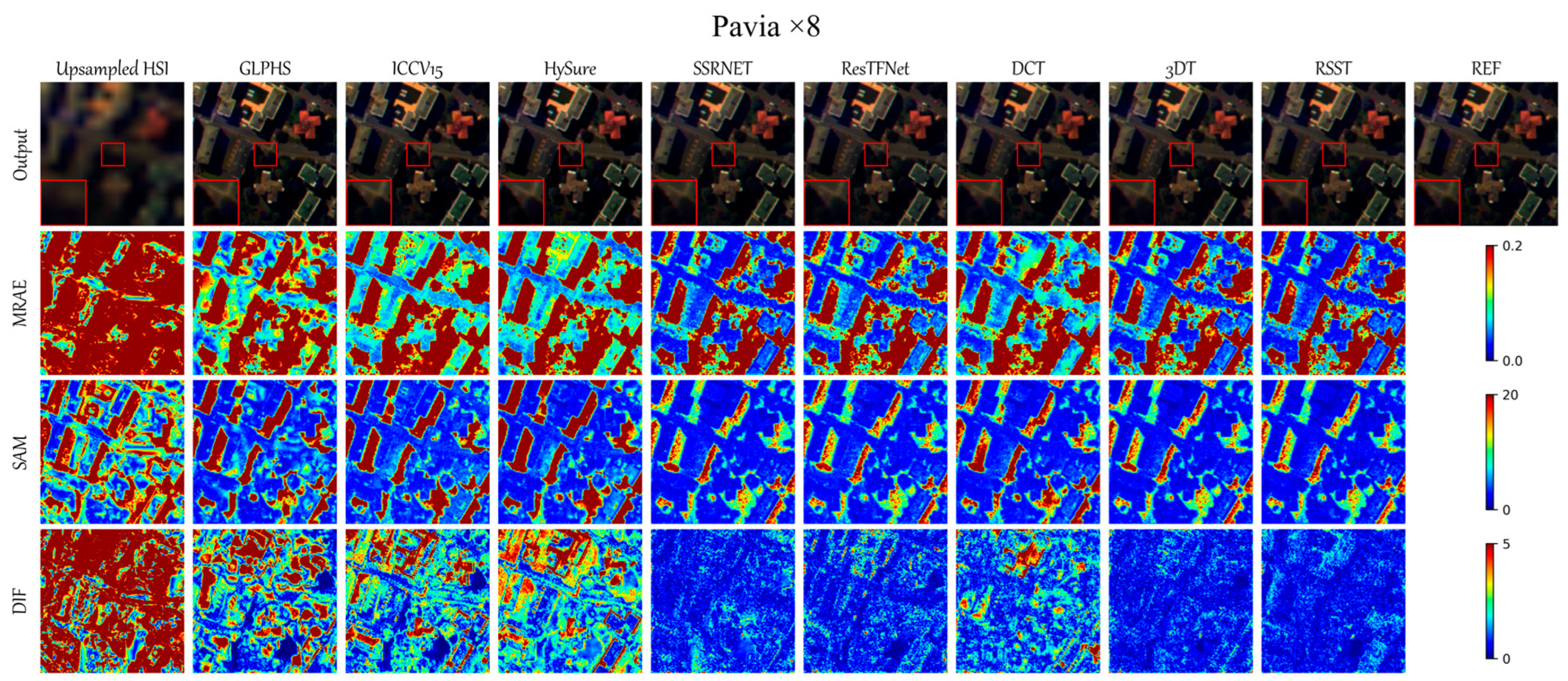

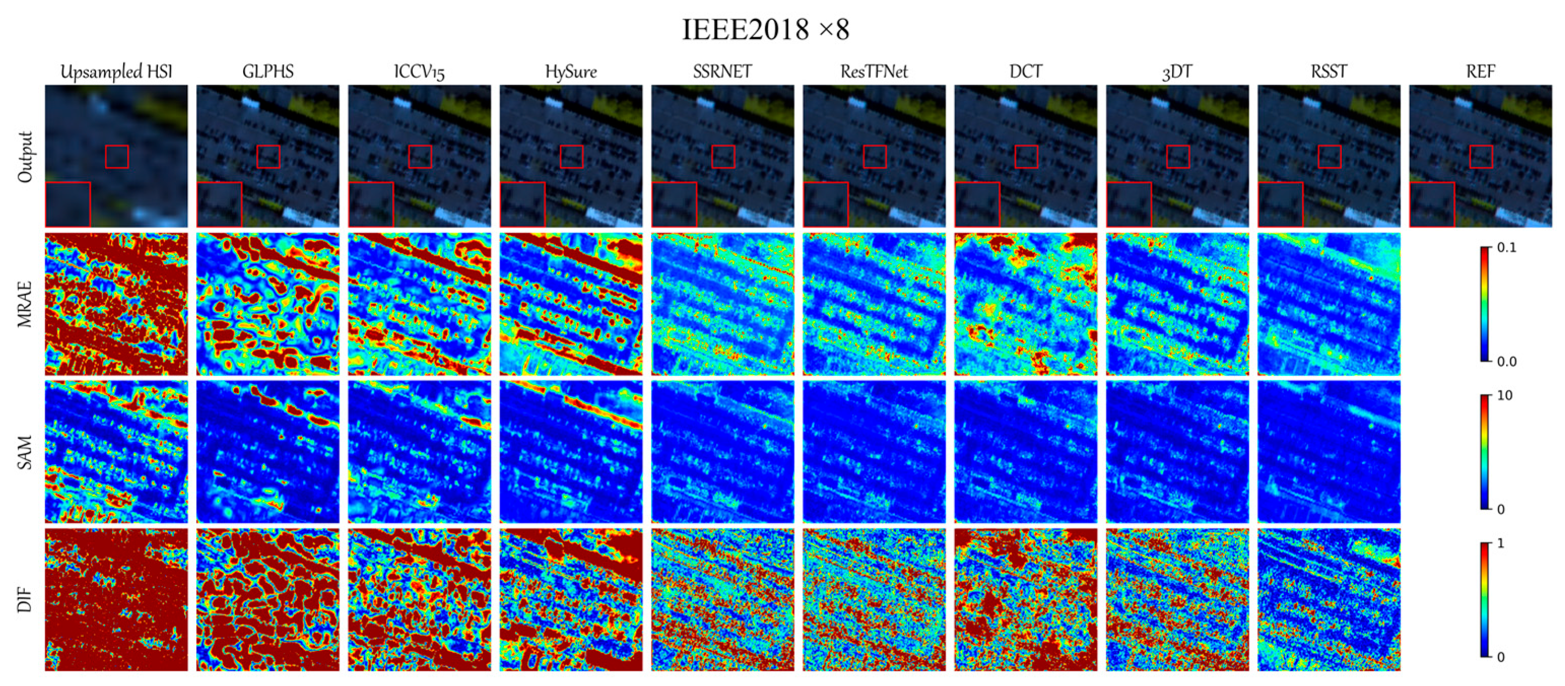


