Long-Term Spatiotemporal Information Extraction of Cultivated Land in the Nomadic Area: A Case Study of the Selenge River Basin

Abstract

The Mongolian Plateau, a region where nomadic and agrarian civilizations intersect, exemplifies regional sustainable development and natural resource utilization through the spatiotemporal distribution of cultivated land. However, large-scale, long-term, high-precision extraction of cultivated land has not been systematically conducted in this area. This study integrated remote sensing technology with machine learning methodologies to develop an automated extraction process based on spectral, textural, and topographical features. We monitored changes in cultivated land across eight time periods from 1990 to 2023 within the Selenge River Basin, utilizing Google Earth Engine and 3527 scenes derived from Landsat and Sentinel satellite imagery. The area of cultivated land fluctuated between 6332.78 km² and 14,799.22 km², representing 2.26% to 5.29% of the total area. Cultivated land exhibited a significant decline prior to 2005 and gradually increased after 2010, largely influenced by agricultural policy reforms. Traditional nomadic areas showed a spatial pattern of reconstruction, characterized by a significant transformation to agricultural land. The overall accuracy exceeded 90%, and kappa coefficients remained above 0.83. Consistency checks and comparisons of different integration methods further validate the feasibility and reliability of the research methods and results. This approach holds promise for application across the entire Mongolian Plateau and other arid and semi-arid regions for monitoring cultivated land dynamics.

1. Introduction

Cultivated land, the most fundamental natural resource and condition for human survival, accounts for 12.6% of global land use and plays a crucial role in sustainable development [1,2]. Large-scale changes in cultivated land significantly impact both global and national agricultural development, as well as the rational utilization of land resources [3]. In the context of the growing scarcity of global cultivated land resources, rapid population growth, and severe environmental pollution, the United Nations has explicitly emphasized in the Sustainable Development Goals (SDGs) the necessity of achieving “No poverty and zero hunger” and “Balancing increased agricultural production and maintaining ecosystem services” [4]. The spatiotemporal distribution of cultivated land is one of the most important parts of agricultural development indicators [5]. Detailed, timely, and accurate monitoring of cultivated land is a crucial prerequisite for food security, land and water resource management, and the assessment of the impact of agriculture on the ecological environment [6].

Traditional methods for obtaining cultivated land information rely primarily on field surveys. Although this approach yields accurate data, it is time consuming and costly for large-scale surveys and the information often becomes outdated, thereby reducing its utility [7]. Remote sensing technology offers a reliable and cost-effective method for long-term, large-scale, and real-time acquisition of cultivated land information. Remote sensing data have proven to be effective in mapping cultivated land [8]. Pittman et al. generated a global cultivated land probability map using MODIS data and a classification tree model that incorporated multi-year indicators [9]. Gumma et al. used MODIS data with spectral matching and decision tree methods to map the distribution of rice-cultivated land in Bangladesh for 2010 [10]. Zhang et al. integrated MODIS with existing statistical data to extract irrigated cultivated land in China from 2000 to 2019 at a 500 m resolution [11]. However, the spatial resolution of MODIS remote sensing data limits its ability to detail the distribution of cultivated land. Medium- and high-resolution remote sensing imagery data are increasingly being used to improve the accuracy of cultivated land mapping [12].

In recent years, the extraction of cultivated land has transitioned from traditional methods to a research paradigm that combines remote sensing cloud platforms with machine learning [13]. Machine learning models, such as the Random Forest (RF) and Support Vector Machine (SVM), have demonstrated high accuracy in handling complex data with high-dimensional feature spaces [14]. The Google Earth Engine (GEE) is currently a leading remote sensing cloud computing platform that does not require users to download data locally. Teluguntla et al. used the Random Forest algorithm and Landsat data to map 30 m resolution crop distributions in Australia and China [15]. Tu et al. generated annual cultivated land datasets for China from 1986 to 2021 by combining time-series Landsat images, automated training sample generation, and machine learning [16]. Xiong et al. used machine learning models as pixel-based classifiers with Sentinel-2 and Landsat-8 data to achieve 30 m resolution cultivated land mapping across Africa [17]. Oliphant et al. employed the Random Forest algorithm on the GEE platform, combining multi-temporal 30 m Landsat data to map cultivated land in Southeast and Northeast Asia [18]. These studies, based on a single machine learning model, primarily focused on spectral time-series features while overlooking other dimensional feature information, resulting in a limited feature space.

Mongolia, located on the northern and central plateau area of Asia, has traditionally been a nomadic country. The northern region of Mongolia is rich in land and water resources, presenting significant potential for agricultural development beyond traditional pastoralism. In recent years, Mongolia has intensified its development and utilization of cultivated land resources. Economic development and policy changes over the past few decades have led to noticeable changes in the cultivated land areas. From 1990 to 2021, 17.6% of land in Mongolia experienced at least one change in type [19]. Considering its unique geographical location and the long-standing risks to ecological security barriers, the overdevelopment of agricultural resources could damage the semi-arid region’s ecosystem. Conversely, insufficient development of cultivated land resources limits the full utilization of the region’s natural resources. Mongolia’s economic development relies primarily on traditional pastoralism and mineral resources, with agriculture not being the primary sector. However, there remains pressure for food security. Large-scale, long-term monitoring of cultivated land has not yet been conducted in this region. Facing dual demands for resource development and ecological security, there is an urgent need for the dynamic monitoring of regional changes in cultivated land.

This study focused on the Selenge River Basin, a representative cultivated land aggregation area in Mongolia, utilizing machine learning algorithms on the GEE platform to construct cultivated land features from spectra, texture, and terrain dimensions. We mapped cultivated land for eight periods from 1990 to 2023, revealing the spatiotemporal distribution patterns of cultivated land in the Selenge River Basin, and the driving forces behind these changes. This study also introduces morphological processing techniques to address the challenges in the post-processing of automated cultivated land extraction.

2. Study Area and Datasets

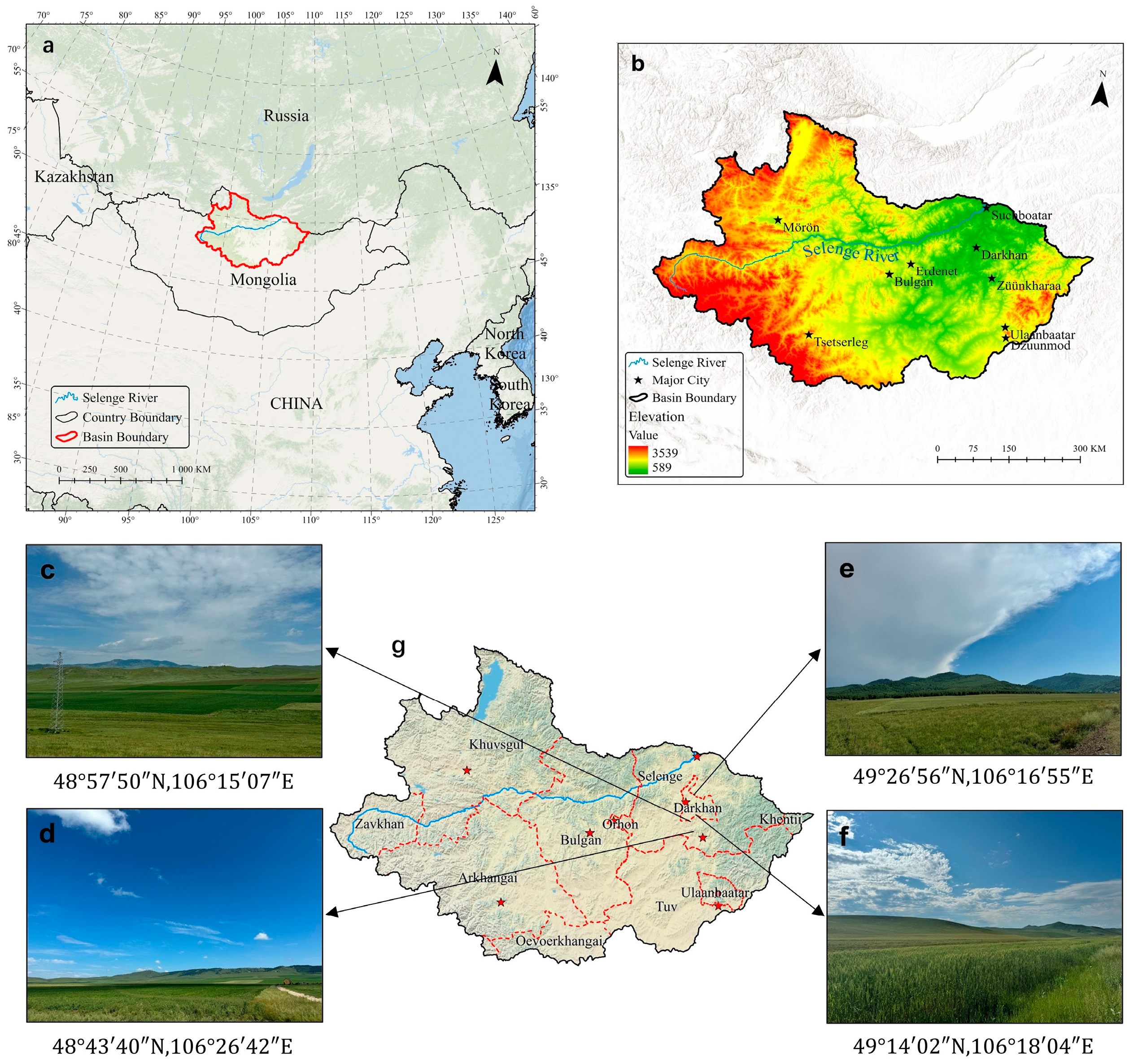
2.1. Study Area

The Selenge River is a major river in the Mongolian Plateau. Originating in the Khangai Mountains in Mongolia, it flows into Lake Baikal in eastern Siberia of Russia, spanning a total length of 1024 km, making it the largest and most voluminous river in Mongolia. The Selenge River Basin (96°50′31″–109°21′32″E, 46°27′50″–51°46′44″N) covers an area of approximately 280,000 km² [20]. The basin occupies the transition zone between forests and grasslands and encompasses 11 provinces, including the Central, Selenga, Darkhan, and Orkhon provinces in Mongolia (Figure 1). The basin’s topography slopes from west to east, with an average elevation of 1600 m. The terrain is characterized by mountainous and hilly regions, with relatively flat central areas. The basin experiences a temperate continental climate with more favorable moisture conditions than those in the Gobi region of southern Mongolia. This research area plays a crucial role in Mongolia’s socio-economic landscape, including the capital city, Ulaanbaatar, the second-largest city, Darkhan, and the third-largest city, Erdenet. These cities account for 69% of the country’s total population and constitute the most agriculturally developed region in Mongolia, producing over 60% of the nation’s agricultural products [21].

2.2. Datasets

Considering the need to study long-term changes and ensure accuracy, this study utilized imagery data from Landsat with 30 m resolution and Sentinel with 10 m resolution. Landsat series satellites are integral to a long-term Earth observation program initiated by NASA and the U.S. Geological Survey (USGS), which monitors changes on the Earth’s surface using satellite remote sensing technology. Sentinel-2 is a part of the European Space Agency (ESA) Copernicus mission and offers high-resolution multispectral imaging primarily for land monitoring. The Landsat 5 TM (Thematic Mapper) was used for 1990, 1995, 2000, 2005, and 2010, offering seven spectral bands, a spatial resolution of 30 m, and a revisit period of 16 days. Data for 2015 were obtained from Landsat 8 OLI (Operational Land Imager). Landsat 8 OLI includes additional spectral bands, totaling 9, which enhance data quality and monitoring capabilities. The spatial resolution is 30 m, with a revisit period of 16 days. To achieve higher resolution extraction results, Sentinel-2 MSI (Multi-Spectral Instrument) data were selected for 2020 and 2023. These data provide a maximum spatial resolution of 10 m, cover 13 spectral bands, and have a minimum revisit period of five days. Given the high latitude of the study area, where winter ground cover is predominantly snow, only images from April to October were selected. Since remotely sensed image data involve different sensors, median synthesis, radiometric correction, and climatic calibration were used to mitigate the temporal consistency problem. The data details are shown in

Table 1. Remote sensing data information.

Satellite	Sensor	Bands	Resolution	Year	Scenes
Landsat 5	Thematic Mapper	B1 Blue	30 m	1990 1995 2000 2005 2010	236 285 305 322 291
		B2 Green	30 m
		B3 Red	30 m
		B4 Nir	30 m
		B5 Swir1	30 m
		B6 Thermal	120 m
		B7 Swir2	30 m
Landsat 8	Operational Land Imager	B1 Coastal	30 m	2015	272
		B2 Blue	30 m
		B3 Green	30 m
		B4 Red	30 m
		B5 Nir	30 m
		B6 Swir1	30 m
		B7 Swir2	30 m
		B8 Pan	15 m
		B9 Cirrus	30 m
Sentinel-2	Multi-Spectral Instrument	B1 Coastal	60 m	2020 2023	1133 683
		B2 Blue	10 m
		B3 Green	10 m
		B4 Red	10 m
		B5 RE1	20 m
		B6 RE2	20 m
		B7 Nir1	20 m
		B8 Nir2	10 m
		B8a Nir3	20 m
		B9 Water vapor	60 m
		B10 Cirrus	60 m
		B11 Swir1	20 m
		B12 Swir2	20 m

, which also lists the number of remote sensing image scenes.

3. Methods

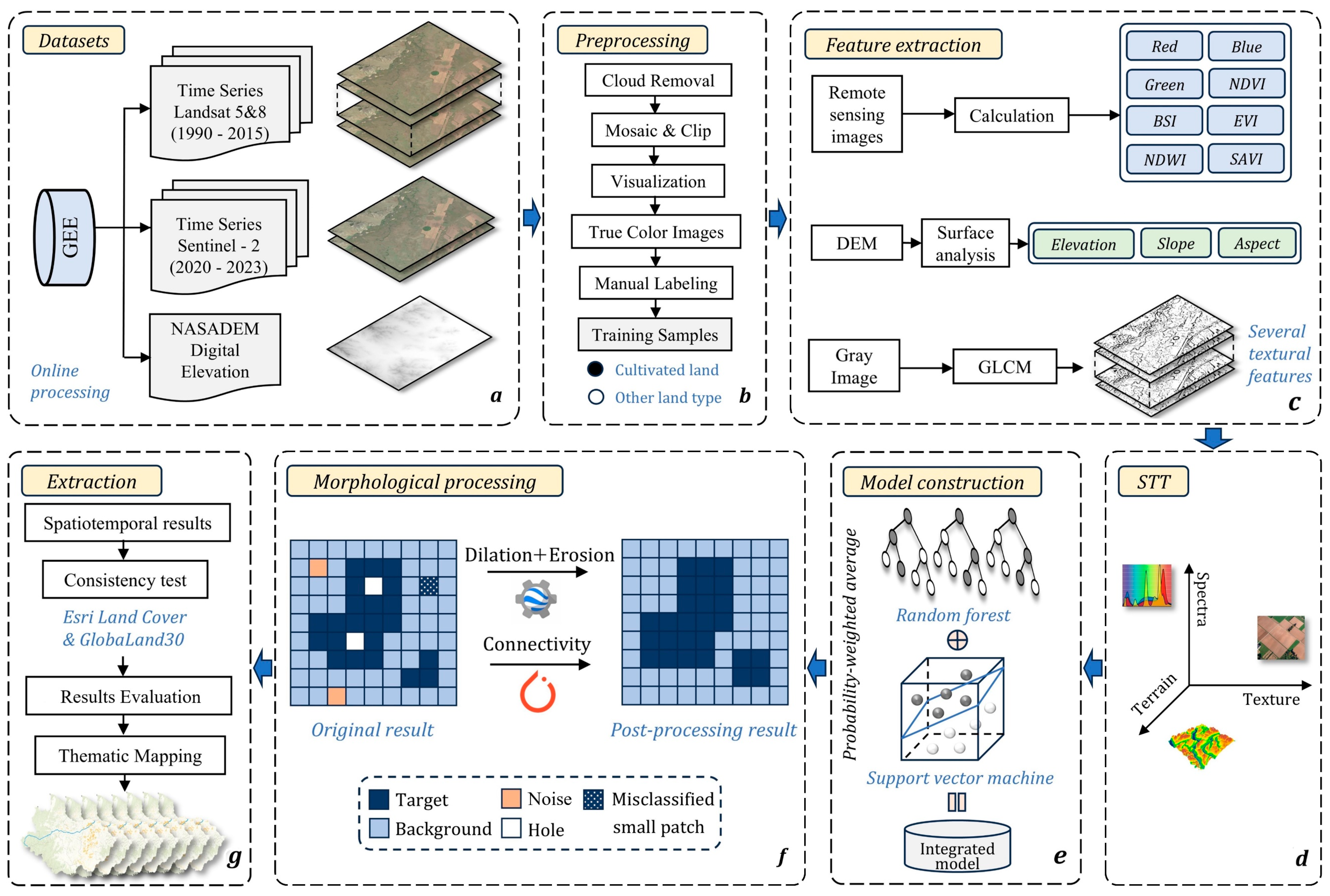
3.1. Overall Framework

Based on a GEE platform and machine learning, an automated cropland extraction technique was developed for large-scale and long-term monitoring. This technique was designed to extract a specific land cover type from complex environments to facilitate tracking and analysis of spatiotemporal dynamics. The technical workflow of this study is illustrated in Figure 2. The workflow is divided into five main parts: data acquisition and preprocessing (a,b), feature extraction (c,d), model construction (e), morphological processing (f), and results extraction (g).

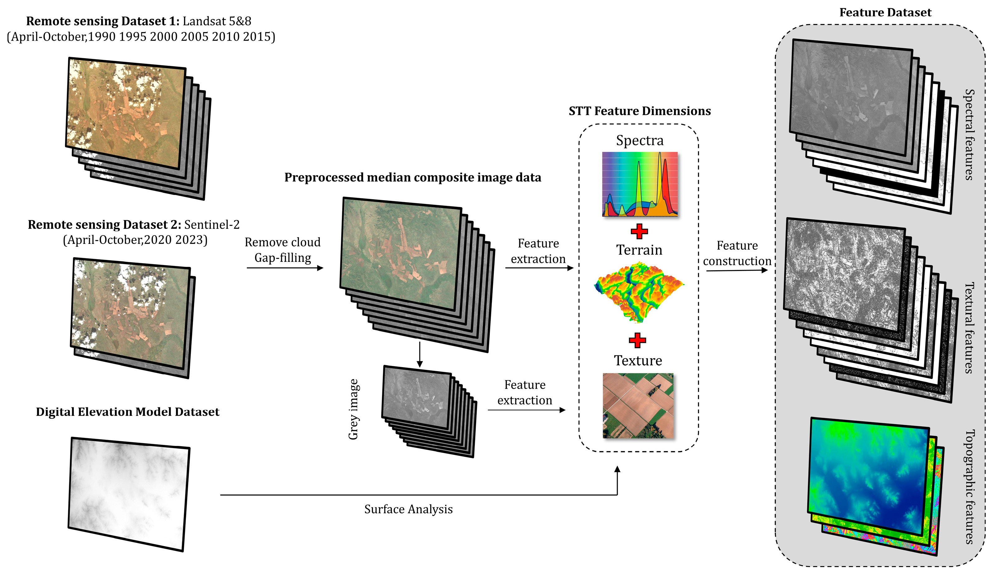
3.2. Feature Space Construction

To highlight the cultivated land target, it is essential to construct a comprehensive feature space that distinguishes between cultivated and non-cultivated land, thereby enhancing heterogeneity and yielding satisfactory extraction results. This study delineated the feature space in three dimensions: spectra, texture, and terrain (STT). The workflow for data processing and feature set construction is illustrated in Figure 3.

It is critical to acknowledge that, in supervised classification, the number of features does not correlate positively with accuracy in a straightforward manner. Considering the Hughes effect, commonly referred to as the curse of dimensionality, accuracy initially increases with the number of features but ultimately declines as dimensionality increases [22,23]. So, we quantitatively assessed the degree of contribution of the initial features to the classification results for the purpose of feature selection and optimization. We used the model interpreter to calculate the importance of each feature, eliminating features with low importance and retaining those with high importance. Different land cover types exhibit varying responses to the absorption and reflection of electromagnetic waves across diverse wavelengths, yielding distinct spectral characteristics [24]. To emphasize these spectral differences, this study utilized the blue, green, and red bands as the characteristic spectral bands.

In complex scenes, incorporating spectral indices to discern subtle differences among land cover types becomes essential. Spectral indices are derived from linear or nonlinear combinations of spectral bands through mathematical computations. These indices enhance the spectral characteristics of land cover and mitigate the redundancy of spectral information. In this study, the selected spectral indices comprise the Normalized Difference Vegetation Index (NDVI), Enhanced Vegetation Index (EVI), Bare Soil Index (BSI), Soil-Adjusted Vegetation Index (SAVI), and Normalized Difference Water Index (NDWI).

Table 2. Spectral indices used in this study.

Spectral Index	Formulation
NDVI	${\displaystyle \frac{\mathrm{N}\mathrm{i}\mathrm{r}-Red}{\mathrm{N}\mathrm{i}\mathrm{r}+Red}}$
BSI	${\displaystyle \frac{\left(\mathrm{R}ed+Swir\right)-\left(Nir+Blue\right)}{\left(\mathrm{R}ed+Swir\right)+\left(Nir+Blue\right)}}$
EVI	${\displaystyle \frac{2.5\left(\mathrm{N}\mathrm{i}\mathrm{r}-Red\right)}{\mathrm{N}\mathrm{i}\mathrm{r}+6Red-7.5Blue+1}}$
SAVI	${\displaystyle \frac{\mathrm{N}\mathrm{i}\mathrm{r}-Red}{\mathrm{N}\mathrm{i}\mathrm{r}+Red+L}}\times \left(1+L\right)$
NDWI	${\displaystyle \frac{\mathrm{G}\mathrm{r}\mathrm{e}\mathrm{e}\mathrm{n}-\mathrm{N}\mathrm{i}\mathrm{r}}{\mathrm{G}\mathrm{r}\mathrm{e}\mathrm{e}\mathrm{n}+\mathrm{N}\mathrm{i}\mathrm{r}}}$

lists the formulas used to calculate each index.

Texture features, classified as global features, characterize the textural properties of land cover. These features are derived from statistical calculations performed on regions comprising multiple pixels, rendering them robust against noise and invariant to rotations. In this study, the gray-level co-occurrence matrix (GLCM) was employed to compute texture features. The formula for generating a gray-scale composite image is as follows:

$$Grey=0.3\times Nir+0.59\times Red+0.11\times Green$$

(1)

Nine specific texture features were selected for this study: Angular Second Moment (ASM), Entropy (ENT), Contrast (CON), Inverse Difference Moment (IDM), Correlation (CORR), Variance (VAR), Sum of Averages (SAVGs), Sum of Variance (SVAR), and Sum of Entropy (SENT).

Table 3. GLCM Texture Feature Description.

Texture Feature	Formulation
Asm(Angular Second Moment)	${\displaystyle \sum _{i=1}^N}{\displaystyle \sum _{j=1}^N}P{\left(i,j\right)}^2$
Ent(Entropy)	$-{\displaystyle \sum _{i=1}^N}{\displaystyle \sum _{j=1}^N}P\left(i,j\right)\mathrm{l}\mathrm{o}\mathrm{g}P\left(i,j\right)$
Con(Contrast)	${\displaystyle \sum _{n=0}^{N-1}}{n}^2{\displaystyle \sum _{i=1}^N}{\displaystyle \sum _{j=1}^N}(P\left(i,j\right)\cdot \left|i-j\right|)$
Idm(Inverse Difference Moment)	${\displaystyle \sum _{i=1}^N}{\displaystyle \sum _{j=1}^N}{\displaystyle \frac{P\left(i,j\right)}{1+{\left(i-j\right)}^2}}$
Corr(Correlation)	${\displaystyle \sum _{i=1}^N}{\displaystyle \sum _{j=1}^N}{\displaystyle \frac{\left(i-{\mu }_i\right)\left(j-{\mu }_j\right)P\left(i,j\right)}{{\sigma }_i{\sigma }_j}}$
Var(Variance)	${\displaystyle \sum _{i=1}^N}{\displaystyle \sum _{j=1}^N}{\left(i-\mu \right)}^{2}P\left(i,j\right)$
Savg(Sum Average)	${\displaystyle \sum _{n=2}^{2N}}n\cdot {\displaystyle \sum _{i=1}^N}{\displaystyle \sum _{j=1}^N}P\left(i,j\right)\cdot \left(i+j\right)$
Svag(Sum Variance)	${\displaystyle \sum _{n=2}^{2N}}{\left(n-SAVG\right)}^2\cdot {\displaystyle \sum _{i=1}^N}{\displaystyle \sum _{j=1}^N}P\left(i,j\right)\cdot \left(i+j\right)$
Sent(Sum Entropy)	$-{\displaystyle \sum _{n=2}^{2N}}{\displaystyle \sum _{i=1}^N}{\displaystyle \sum _{j=1}^N}P\left(i,j\right)\cdot \mathrm{l}\mathrm{o}\mathrm{g}\left(P\left(i,j\right)\cdot \left(i+j\right)\right)$

lists the formulas used to calculate each texture feature.

$P\left(i,j\right)$ represents the value at position $\left(i,j\right)$ in GLCM; $N$ represents the dimension of the GLCM; $n$ represents the pixel value difference; ${\mu }_i$ and ${\mu }_j$ represent the means of gray levels $i$ and $j$; ${\sigma }_i$ and ${\sigma }_j$ represent the standard deviations of gray levels $i$ and $j$; $i$ and $j$ represent gray levels.

In addition to the aforementioned planar features, this study incorporated terrain features. Utilizing the Digital Elevation Model (DEM), surface analysis was performed to derive the elevation, slope, and aspect factors, which were subsequently included in the feature dataset. In order to avoid excessive dimensionality, this study screened features by ranking them by importance. After multiple experimental verifications, it was found that the top five important features were NDVI, DEM, BSI, EVI, and Blue.

3.3. Sample Generation and Selection

Visual interpretation of remote sensing images was employed during the selection of the training samples. The samples were categorized as positive or negative. To ensure representativeness, the positive samples encompassed the majority of areas where cultivated land was distributed. Negative samples are broadly selected to include all types of non-cultivated land. This sampling strategy inevitably results in an imbalance between the number of positive and negative samples. A random selection method was used to reduce model bias caused by this imbalance.

Table 4. Number of positive and negative samples at each time.

Year	Cultivated Land	Non-Cultivated Land	Total
1990	248	372	620
1995	205	306	511
2000	200	272	472
2005	211	429	640
2010	272	490	762
2015	302	458	760
2020	265	466	731
2023	240	493	733

shows the number of samples for each time phase. In order to reduce the artificial subjectivity of sample selection, the Euclidean distance in the feature space was introduced to quantitatively assess the distribution and degree of separability of the samples.

3.4. Machine Learning Model Construction

To emphasize the spectral features and augment the contribution of spectral indices in the classifier, the minimum, maximum, mean, and standard deviations of the NDVI, BSI, and EVI were incorporated as auxiliary spectral features during model training. Each feature layer was spatially stacked to create a three-dimensional feature set (L × R × N, where L and R denote the row and column counts of the feature layers, respectively, and N represents the number of features). Ensuring a unified geographical coordinate system and consistent scaling is a prerequisite for this procedure.

This study employs a pixel-level classification strategy utilizing Random Forest (RF) and Support Vector Machine (SVM) as classifiers. The model algorithms are implemented on the GEE platform. The RF model is trained by constructing multiple decision trees and classifies them based on a combination of results from these trees, providing high accuracy and stability. Assuming that there are $T$ decision trees $h_1, h_2, \dots h_T$, for an input sample $x$, the classification result $H\left(x\right)$ of the Random Forest is the mode of the classification results from all decision trees, that is

$$H\left(x\right)=mode\left\{h_1\left(x\right), h_2\left(x\right), \dots h_T\left(x\right)\right\}$$

(2)

The SVM model classifies data points by determining the optimal hyperplane that separates different classes in a high-dimensional space. Given a training dataset ${(x}_1, y_1), {(x}_2, y_2), \dots {(x}_n, y_n)$, where $x_i$ are feature vectors and $y_i\in \{-1, 1\}$ are class labels, SVM finds the optimal hyperplane by solving the following optimization problem:

$$\begin{array}{ll} & {\mathrm{m}\mathrm{i}\mathrm{n}}_{\mathrm{w},b,\xi }{\displaystyle \frac{1}{2}}\parallel \mathrm{w}{\parallel }^2+C{\displaystyle \sum _{i=1}^n}{\xi }_i\\ & \mathrm{s}\mathrm{u}\mathrm{b}\mathrm{j}\mathrm{e}\mathrm{c}\mathrm{t} \mathrm{t}\mathrm{o} y_i\left(\mathrm{w}\cdot x_i+b\right)\ge 1-{\xi }_i, {\xi }_i\ge 0\end{array}$$

(3)

where $\mathrm{w}$ is the normal vector to the hyperplane, $b$ is the bias, $\xi$ is the slack variables, and $C$ is the regularization parameter.

As previously mentioned, samples are randomly selected in equal numbers, and different training outcomes can be obtained when inputted into the model. In this study, each model was iteratively trained 20 times, and the parameters yielding the highest accuracy in the validation set were selected as the optimal parameters for that model. This ensured that the best results were obtained, thereby mitigating the randomness of a single training session. In the binary classification problem of this study, machine learning models classified each pixel individually, with each pixel value representing the probability of belonging to a certain class. Therefore, based on this principle, the classification results of RF and SVM can be averaged to integrate the results of different machine learning models. This approach improves the accuracy and robustness of the classification results through ensemble machine learning.

The classification results from RF, $h_{RF}\left(x\right)$, and the classification results from SVM, $h_{SVM}\left(x\right)$, can be combined using weighted integration. The weighted integration result, $h_{Weighted}\left(x\right)$, was obtained by rounding the weighted sum of both results:

$${\mathrm{H}}_{\mathrm{Weighted}}\left(\mathrm{x}\right)=\mathrm{r}\mathrm{o}\mathrm{u}\mathrm{n}\mathrm{d}\left({\mathrm{w}}_1\cdot {\mathrm{h}}_{\mathrm{R}\mathrm{F}}\left(\mathrm{x}\right)+{\mathrm{w}}_2\cdot {\mathrm{h}}_{\mathrm{S}\mathrm{V}\mathrm{M}}\left(\mathrm{x}\right)\right)$$

(4)

where ${\mathrm{w}}_1$ and ${\mathrm{w}}_2$ are the weights for RF and SVM, respectively, such that ${\mathrm{w}}_1+{\mathrm{w}}_2=1$. In this study, ${\mathrm{w}}_1$ was set to 0.7 and ${\mathrm{w}}_2$ was set to 0.3. The selection of weight ratio for integrating RF and SVM models was rigorously validated through iterative training and sensitivity analysis. The model integration effect was best when the weight was 0.7:0.3.

3.5. Morphological Post-Processing

For large-scale mapping, the resulting raster data may contain noise, holes, and small patches, which affect the coherence and significantly interfere with the accuracy and effectiveness. Therefore, morphological post-processing is essential to obtain the initial results. Morphological post-processing in this study was implemented using GEE and PyTorch (3.6). It primarily utilizes the ‘focalMax’ and ‘focalMin’ functions of the Image class in GEE and the ‘SieveFilter’ function of the GDAL library. The morphological post-processing workflow consisted of two main steps. Step 1 involves the use of mathematical morphology operations, specifically closing operations (dilation followed by erosion), to fill small internal gaps within the raster and smooth the boundaries. Despite the morphological filtering in the first step, small patches in the raster results remained unresolved. Step 2 involved local processing in PyTorch, including connectivity calculations and the removal of small patches. Connectivity was computed using 4 neighborhoods to identify and label all connected pixel groups within the raster, allowing the deletion of regions smaller than a given threshold and effectively removing isolated small patches and noise. We selected a 90 m × 90 m window for smoothing the edge for the last step. This process just tries to make the edge of the final map more smooth and avoid some sawtooth or separate pieces in or near the edge of the map. This window was an optimized size in similar studies [25].

4. Results

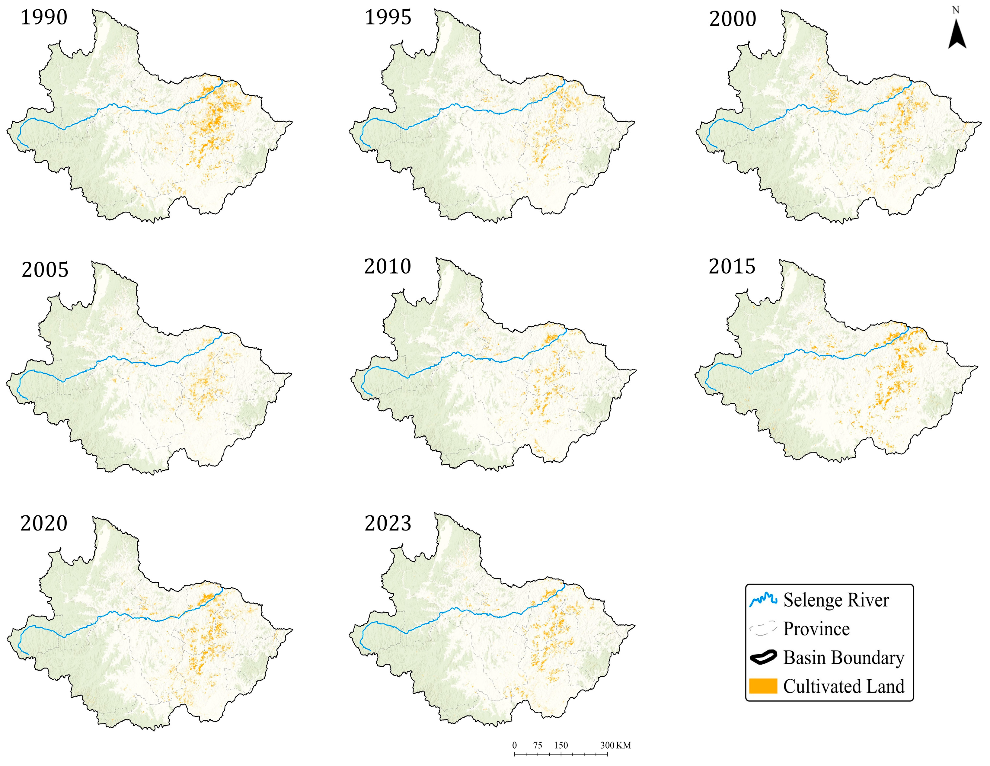
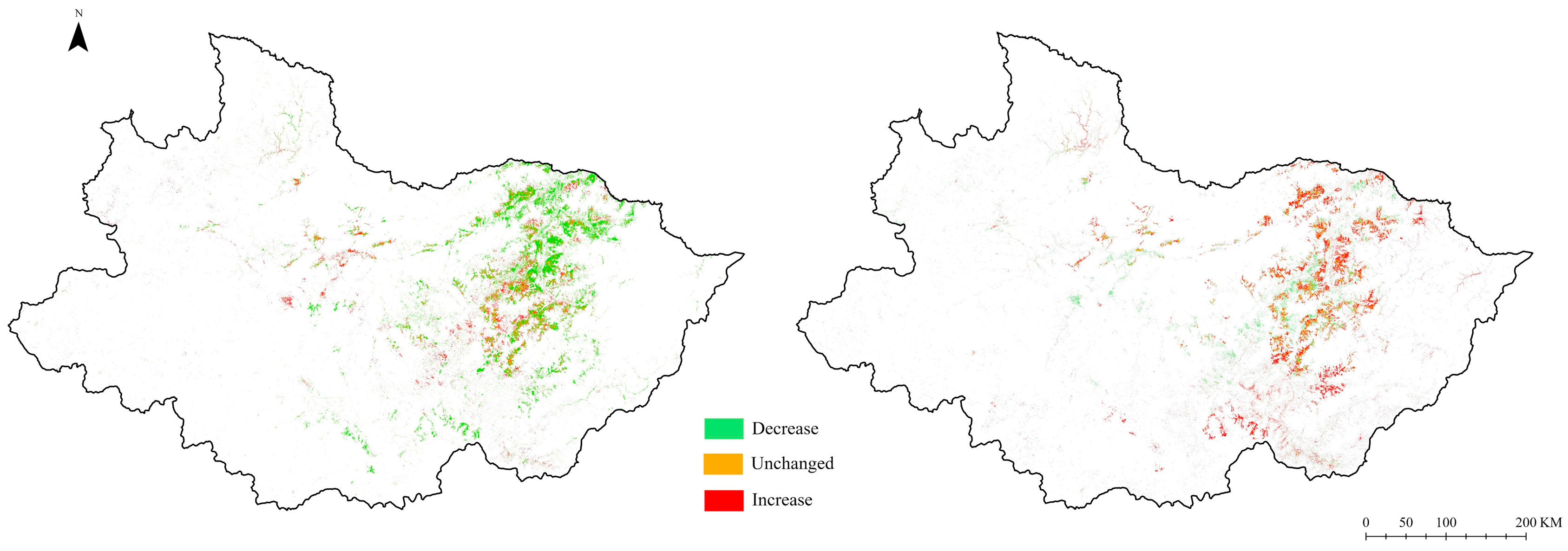
4.1. Analysis of Temporal and Spatial Distribution Patterns

The extracted cultivated land results were mapped using ArcGIS Pro. From 1990 to 2023, the spatial distribution pattern of cultivated land in the Selenge River Basin remains relatively stable, with higher and lower concentrations in the northeast and southwest, respectively. Large areas of cultivated land are located near the northern Mongolian cities of Sukhbaatar and Darkhan. Figure 4 shows the spatial and temporal distribution of cultivated land throughout the Selenge River Basin. Overall, the temporal and spatial distribution of cultivated land showed a significant reduction from 1990 to 2005 and a gradual increase from 2010 to 2023, accompanied by a recent slowing of the overall expansion trend and some reductions in local areas, especially in marginal regions of the basin.

In order to better show the increase or decrease in cultivated land change, the results of cultivated land extraction were change-detected and mapped. The year 2005 is a key point in the trend of cultivated land change in the study area. Figure 5 shows the change in cultivated land before and after 2005 (1990–2005, 2005–2023). Cultivated land declined sharply before 2005 and recovered gradually after 2005. The pattern of cultivated land change shifted from a recessionary contraction in the earlier period to an agglomeration expansion in the later period.

4.2. Quantitative Statistics on Area Changes

To quantitatively analyze the changes in the cultivated land area, the extracted results were subjected to grid statistics. The analysis calculated the number of grid cells classified as cultivated land, with each grid cell of known size (30 × 30 m or 10 × 10 m), allowing the determination of the total cultivated land area for each time phase. Figure 6 presents bar and line charts of the changes in cultivated land area, while

Table 5. Cultivated land area in the Selenge River Basin statistics by region (km²).

	Arkhangai	Bulgan	Darkhan	Zavkhan	Khentii	Khuvsgul	Orhon	Oevoerkhangai	Selenge	Tuv	Ulaanbaatar	Sum
1990	337.01	1571.68	1241.69	15.70	28.22	569.19	97.60	162.78	7807.47	2830.40	137.48	14,799.22
1995	10.97	1051.86	687.96	2.20	4.61	237.86	42.19	2.53	6721.63	2570.58	11.75	11,344.14
2000	205.40	1666.88	709.70	9.28	9.12	864.42	43.81	17.37	4034.30	2183.65	66.45	9810.37
2005	156.96	973.53	284.97	28.85	0.01	505.56	34.75	12.82	2886.49	1438.40	10.42	6332.78
2010	69.35	1067.92	320.94	65.11	0.30	546.28	44.42	8.24	3432.81	2070.90	28.51	7654.78
2015	247.63	1181.77	482.68	21.66	1.66	409.24	39.89	47.53	3599.06	1976.48	11.30	8018.91
2020	120.98	988.42	407.89	3.01	0.00	385.12	82.10	149.73	4016.56	2222.68	33.21	8409.69
2023	181.96	754.33	642.79	11.44	2.74	480.72	54.98	63.25	4091.14	2701.43	23.27	9008.04

records the changes in cultivated land area within the basin and each province.

The cultivated land area in the Selenge River Basin exhibited a significant initial decrease, followed by a stable increase. In 1990, the cultivated land area peaked at 14,799.22 km², whereas in 2005, it reached its lowest point at 6332.78 km². The most substantial decrease occurred from 2000 to 2005, with a reduction of 35.45% compared with 2000. The largest increase, 20.88%, occurred between 2005 and 2010. From 2015 to 2023, the cultivated land area steadily increases, averaging an increment of 451.08 km² every five years, with an average growth rate of 5.58%. The trends in each province within the basin were generally aligned with the overall trends. Selenge has the largest cultivated land area, followed by Tuv, Bulgan, and Khuvsgul.

4.3. Accuracy Assessment

For the quantitative evaluation of the results, this study used Overall Accuracy (OA) and kappa as standards to evaluate the model’s ability to identify and extract cultivated land. The confusion matrix was calculated for the cultivated land extraction results of all eight time phases. The accuracy evaluation metrics are summarized in

Table 6. Cultivated land extraction accuracy.

Year	OA	Kappa
1990	0.9121	0.8410
1995	0.9072	0.8325
2000	0.9058	0.8230
2005	0.9023	0.8121
2010	0.9376	0.8673
2015	0.9016	0.8152
2020	0.9272	0.8573
2023	0.9123	0.8531

. The highest extraction accuracy was achieved in 2010, with an OA of 0.9376 and a kappa of 0.8673. We calculated the average accuracy of eight results, with an overall average accuracy (Avg OA) of 0.9266 and an average kappa (Avg Kappa) of 0.8376. These results demonstrate the reliability of the cultivated land extraction method employed in this study, which accurately reflects the spatiotemporal distribution of cultivated land in the study area.

5. Discussion

5.1. Evaluation and Validation of Results

To further demonstrate the reliability and accuracy of the cultivated land extraction results of this study, we selected the global land use data products ESRI Land Cover (85% accuracy) [26] and GlobaLand30 (80–85% accuracy) [27] as references. Consistency checks were conducted using linear programming, and quantitative measurements were performed by calculating the Coefficient of Determination (R²), Root Mean Squared Error (RMSE), and Mean Absolute Error (MAE). A direct comparison of the entire basin area cannot describe the local consistency, necessitating a regional subdivision of the basin. Due to the lack of provincial cultivated land statistics for this basin and the fact that some provinces are not fully contained within it, administrative divisions are not feasible for this purpose. Instead, this study used the Generate Tessellation tool in ArcGIS Pro to create a hexagonal grid, as shown in Figure 7, with each hexagon covering an area of 500 km².

Consistency checks were conducted by calculating the cultivated land area within each hexagon. Figure 8 presents the results of consistency checks, validating the cultivated land extraction results for 2000, 2010, 2020, and 2023. For 2010 and 2020, the R² values were all greater than 0.85, with the highest at 0.9130 and the lowest at 0.8138. The average RMSE was 20.8371 and the average MAE was 59.6595. According to these results, there is good consistency between the cultivated land extraction results from this study and mainstream land use datasets, demonstrating the feasibility of the research methods and the reliability of the data. While consistency checks with GlobaLand30 and ESRI Land Cover demonstrate alignment (R² > 0.8), localized discrepancies may arise due to differences in classification schemes or temporal mismatches.

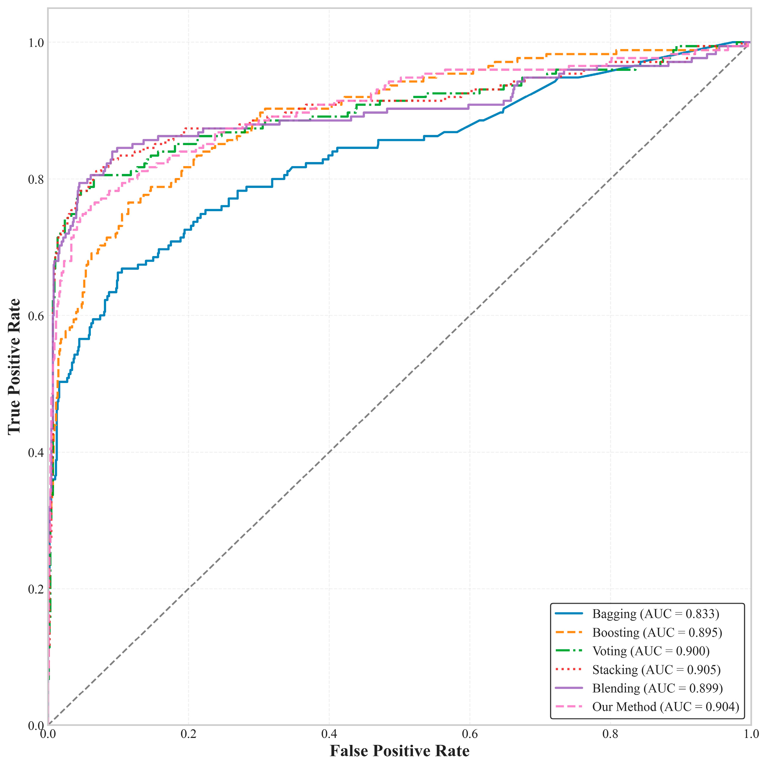
5.2. Comparative Analysis of Methodological Advantages

The proposed integrated machine learning and morphological post-processing system demonstrated significant superiority in large-scale, long-term cultivated land information extraction, primarily in the following aspects: (1) achieving the integration of multiple machine learning models, (2) completing samples selection and constructing the STT feature space, and (3) proposing a complete morphological post-processing system. While employing multi-source data and multi-scale analysis, related studies did not delve deeply into model integration [28,29,30]. Moreover, most current studies on cultivated land extraction overlook the post-processing of the results, leading to an inaccurate reflection of cultivated land distribution.

For the reliability of the weighted average integration model, we selected the integration learning models in recent years for comparison (

Table 7. Comparison of different model integrate methods.

Integrated Strategy	Base Models	Advantages/Disadvantages	OA	Kappa
Bagging [31]	RF	Limited bias reduction; computationally intensive with many models	0.8945	0.8274
Boosting [32]	RF; XGBoost	Prone to overfitting noisy data; sensitive to outliers	0.9056	0.8312
Voting [33]	RF; SVM; KNN	Performance bounded by weakest base model	0.8761	0.8012
Stacking [34]	RF; XGBoost; GBM	Risk of meta-earner overfitting; complex training and data splitting	0.9264	0.8671
Blending [35]	XGBoost; SVM	Require careful validation-set tuning	0.8614	0.7890
Our method	RF, SVM	Simple and efficient; highly stable; avoid overfitting; offers interpretability and discriminative power	0.9123	0.8531

). We conducted experiments using the latest 2023 data to compare different integration methods. The results showed that our method has the high OA (0.9123), just lower than the stacking method, which has the highest OA and kappa. But the training process of the stacking method model was relatively complex. Unlike with stacking and other integrated methods, our method does not require training the meta-learner, which reduces the computational effort and avoids overfitting on finite samples. Fixed weights clarify the contribution of each model, facilitating model diagnosis and policy-oriented decision support. We plotted ROC (Receiver Operating Characteristic) curves and calculated AUC (Area Under Curve) for different methods to facilitate further quantitative comparison (Figure 9). In contrast, our method demonstrated advantages over other methods in terms of model construction, training efficiency, and result accuracy.

5.3. Analysis of Drivers of Spatial and Temporal Change

The spatial center of cultivated land in the Selenge River Basin did not undergo significant changes, with the main distribution areas consistently located in the eastern and northern regions. There were two distinct temporal changes in the cultivated land area. The first was the significant reduction in the area from 1990 to 2005, which was primarily influenced by policy shifts during the late socialist period and the transition to a market economy. In the 1990s, following the dissolution of the former Soviet Union, Mongolia lost crucial economic support and technical assistance, leading to disruptions in the agricultural supply, aging agricultural machinery, and the gradual dismantling of state farms. Additionally, increased international trade barriers raise agricultural production costs and reduce profitability, resulting in the widespread abandonment of cultivated land [25,36]. While direct policy metrics are unavailable, indirect evidence highlights institutional collapse and diminished state support as key drivers. A 60% reduction in functional tractors [37] and a 40% rise in agricultural imports [38] critically impaired cultivation capacity during this period. Concurrently, this period is likely to experience accelerated urbanization, with urban expansion encroaching on cultivated land [21].

The second period is a stable increase in cultivated land area from 2010 to 2023, primarily due to national policy adjustments, changes in market demand, and increased investment. For instance, in the 21st century, the Mongolian government implemented reclamation plans and South–South cooperation initiatives aimed at encouraging agricultural production by providing machinery, technical support, and easier market access. These policies contribute to the recovery and increase in cultivated land. Additionally, with a growing emphasis on food security both domestically and internationally, Mongolia has focused on enhancing agricultural output, increasing agricultural investment, and improving cultivation techniques and management to meet population growth and market demand. Furthermore, increased international cooperation and investment, particularly economic cooperation with neighboring countries such as China, South Korea, Japan, and Russia, will provide financial and technical support for Mongolia’s agricultural development. Overall, the changes in Mongolia’s cultivated land area reflect the complex interplay between economic policies, market demand, and environmental factors.

6. Conclusions

This study utilized multi-temporal remote sensing images to automatically extract cultivated land in the Selenge River Basin of Mongolia from 1990 to 2023, using the constructed STT feature space and integrated machine learning models. Comprehensive monitoring and analysis of temporal and spatial changes in cultivated land were conducted, resulting in multi-temporal–spatial distribution maps for the Selenge River Basin. The study realized the automatic extraction of long-term and large-scale cultivated land and introduced sample quantitative evaluation indexes and morphological processing methods to improve the processing workflow. The results indicated that cultivated land in the basin undergoes a dynamic process of first decreasing and then increasing. The cultivated land area experienced a significant reduction in the 1990s but has gradually and steadily increased since 2010, with the largest area observed in 1990 and the smallest in 2005. This study successfully achieved a high-precision extraction of cultivated land, with an overall accuracy (OA) of 0.9266 and a kappa coefficient of 0.8376. A comparison with other global land use data and consistency checks yielded an average R² of 0.8569, validating the feasibility of the methods. The comparison results of different integration methods show the reliability and efficiency of the weighted average method. The proposed cultivated land extraction workflow, based on an integrated model and STT, demonstrated strong generalization capabilities, making it extendable to the entire Mongolian Plateau and other arid and semi-arid regions.

References

1. Bren d’Amour, C.; Reitsma, F.; Baiocchi, G.; Barthel, S.; Guneralp, B.; Erb, K.H.; Haberl, H.; Creutzig, F.; Seto, K.C. Future urban land expansion and implications for global croplands. Proc. Natl. Acad. Sci. USA 2017, 114, 8939–8944. [Google Scholar] [CrossRef] [PubMed]
2. Rudel, T.K.; Schneider, L.; Uriarte, M.; Turner, B.L.; DeFries, R.; Lawrence, D.; Geoghegan, J.; Hecht, S.; Ickowitz, A.; Lambin, E.F.; et al. Agricultural intensification and changes in cultivated areas, 1970–2005. Proc. Natl. Acad. Sci. USA 2009, 106, 20675–20680. [Google Scholar] [CrossRef] [PubMed]
3. Zhang, S.; Zhang, H.; Gu, X.; Liu, J.; Yin, Z.; Sun, Q.; Wei, Z.; Pan, Y. Monitoring the spatio-temporal changes of non-cultivated land via long-time series remote sensing images in xinghua. IEEE Access 2022, 10, 84518–84534. [Google Scholar] [CrossRef]
4. Bizikova, L.; Jungcurt, S.; McDougal, K.; Tyler, S. How can agricultural interventions enhance contribution to food security and sdg 2.1? Glob. Food Secur. 2020, 26, 100450. [Google Scholar] [CrossRef]
5. Xiong, J.; Thenkabail, P.S.; Gumma, M.K.; Teluguntla, P.; Poehnelt, J.; Congalton, R.G.; Yadav, K.; Thau, D. Automated cropland mapping of continental africa using google earth engine cloud computing. ISPRS J. Photogramm. Remote Sens. 2017, 126, 225–244. [Google Scholar] [CrossRef]
6. Waldner, F.; Canto, G.S.; Defourny, P. Automated annual cropland mapping using knowledge-based temporal features. ISPRS J. Photogramm. Remote Sens. 2015, 110, 1–13. [Google Scholar] [CrossRef]
7. Liu, W.; Wu, Z.; Luo, J.; Sun, Y.; Wu, T.; Zhou, N.; Hu, X.; Wang, L.; Zhou, Z. A divided and stratified extraction method of high-resolution remote sensing information for cropland in hilly and mountainous areas based on deep learning. Acta Geod. Cartogr. Sin. 2021, 50, 105–116. [Google Scholar]
8. Potapov, P.; Turubanova, S.; Hansen, M.C.; Tyukavina, A.; Zalles, V.; Khan, A.; Song, X.P.; Pickens, A.; Shen, Q.; Cortez, J. Global maps of cropland extent and change show accelerated cropland expansion in the twenty-first century. Nat. Food 2022, 3, 19–28. [Google Scholar] [CrossRef]
9. Pittman, K.; Hansen, M.C.; Becker-Reshef, I.; Potapov, P.V.; Justice, C.O. Estimating global cropland extent with multi-year modis data. Remote Sens. 2010, 2, 1844–1863. [Google Scholar] [CrossRef]
10. Gumma, M.K.; Thenkabail, P.S.; Maunahan, A.; Islam, S.; Nelson, A. Mapping seasonal rice cropland extent and area in the high cropping intensity environment of bangladesh using modis 500 m data for the year 2010. ISPRS J. Photogramm. Remote Sens. 2014, 91, 98–113. [Google Scholar] [CrossRef]
11. Zhang, C.; Dong, J.; Ge, Q. Mapping 20 years of irrigated croplands in china using modis and statistics and existing irrigation products. Sci. Data 2022, 9, 407. [Google Scholar] [CrossRef] [PubMed]
12. Dong, J. State of the art and perspective of agricultural land use remote sensing information extraction. J. Geo-Inf. Sci. 2020, 22, 772–783. [Google Scholar]
13. Azzari, G.; Lobell, D.B. Landsat-based classification in the cloud: An opportunity for a paradigm shift in land cover monitoring. Remote Sens. Environ. 2017, 202, 64–74. [Google Scholar] [CrossRef]
14. Maxwell, A.E.; Warner, T.A.; Fang, F. Implementation of machine-learning classification in remote sensing: An applied review. Int. J. Remote Sens. 2018, 39, 2784–2817. [Google Scholar] [CrossRef]
15. Teluguntla, P.; Thenkabail, P.S.; Oliphant, A.; Xiong, J.; Gumma, M.K.; Congalton, R.G.; Yadav, K.; Huete, A. A 30-m landsat-derived cropland extent product of australia and china using random forest machine learning algorithm on google earth engine cloud computing platform. ISPRS J. Photogramm. Remote Sens. 2018, 144, 325–340. [Google Scholar] [CrossRef]
16. Tu, Y.; Wu, S.; Chen, B.; Weng, Q.; Bai, Y.; Yang, J.; Yu, L.; Xu, B. A 30 m annual cropland dataset of china from 1986 to 2021. Earth Syst. Sci. Data 2024, 16, 2297–2316. [Google Scholar] [CrossRef]
17. Xiong, J.; Thenkabail, P.; Tilton, J.; Gumma, M.; Teluguntla, P.; Oliphant, A.; Congalton, R.; Yadav, K.; Gorelick, N. Nominal 30-m cropland extent map of continental africa by integrating pixel-based and object-based algorithms using sentinel-2 and landsat-8 data on google earth engine. Remote Sens. 2017, 9, 1065. [Google Scholar] [CrossRef]
18. Oliphant, A.J.; Thenkabail, P.S.; Teluguntla, P.; Xiong, J.; Gumma, M.K.; Congalton, R.G.; Yadav, K. Mapping cropland extent of southeast and northeast asia using multi-year time-series landsat 30-m data using a random forest classifier on the google earth engine cloud. Int. J. Appl. Earth Obs. Geoinf. 2019, 81, 110–124. [Google Scholar] [CrossRef]
19. Hao, J.; Lin, Q.; Wu, T.; Chen, J.; Li, W.; Wu, X.; Hu, G.; La, Y. Spatial–temporal and driving factors of land use/cover change in mongolia from 1990 to 2021. Remote Sens. 2023, 15, 1813. [Google Scholar] [CrossRef]
20. Zhou, J.; Wang, J. Ecological security assessment of selenge river basin in mongolia based on psr model. J. Agric. Big Data 2023, 5, 87–94. [Google Scholar]
21. Ren, Y.; Li, Z.; Li, J.; Ding, Y.; Miao, X. Analysis of land use/cover change and driving forces in the selenga river basin. Sensors 2022, 22, 1041. [Google Scholar] [CrossRef] [PubMed]
22. Taskin, G.; Kaya, H.; Bruzzone, L. Feature selection based on high dimensional model representation for hyperspectral images. IEEE Trans. Image Process. 2017, 26, 2918–2928. [Google Scholar] [CrossRef] [PubMed]
23. Hughes, G. On the mean accuracy of statistical pattern recognizers. IEEE Trans. Inf. Theory 1968, 14, 55–63. [Google Scholar] [CrossRef]
24. Bhargava, A.; Sachdeva, A.; Sharma, K.; Alsharif, M.H.; Uthansakul, P.; Uthansakul, M. Hyperspectral imaging and its applications: A review. Heliyon 2024, 10, e33208. [Google Scholar] [CrossRef]
25. Sankey, T.T.; Massey, R.; Yadav, K.; Congalton, R.G.; Tilton, J.C. Post-socialist cropland changes and abandonment in mongolia. Land Degrad. Dev. 2018, 29, 2808–2821. [Google Scholar] [CrossRef]
26. Karra, K.; Kontgis, C.; Statman-Weil, Z.; Mazzariello, J.C.; Mathis, M.; Brumby, S.P. Global land use/land cover with sentinel 2 and deep learning. In Proceedings of the 2021 IEEE International Geoscience and Remote Sensing Symposium IGARSS, Brussels, Belgium, 11–16 July 2021; pp. 4704–4707. [Google Scholar]
27. Jun, C.; Ban, Y.; Li, S. Open access to earth land-cover map. Nature 2014, 514, 434. [Google Scholar] [CrossRef] [PubMed]
28. Qiu, B.; Liu, B.; Tang, Z.; Dong, J.; Xu, W.; Liang, J.; Chen, N.; Chen, J.; Wang, L.; Zhang, C.; et al. National-scale 10-m maps of cropland use intensity in china during 2018–2023. Sci. Data 2024, 11, 691. [Google Scholar] [CrossRef]
29. Liu, L.; Kang, S.; Xiong, X.; Qin, Y.; Wang, J.; Liu, Z.; Xiao, X. Cropping intensity map of china with 10 m spatial resolution from analyses of time-series landsat-7/8 and sentinel-2 images. Int. J. Appl. Earth Obs. Geoinf. 2023, 124, 103504. [Google Scholar] [CrossRef]
30. Shi, K.; Yang, Q.; Li, Y.; Sun, X. Mapping and evaluating cultivated land fallow in southwest china using multisource data. Sci. Total Environ. 2019, 654, 987–999. [Google Scholar] [CrossRef]
31. Svoboda, J.; Štych, P.; Laštovička, J.; Paluba, D.; Kobliuk, N. Random forest classification of land use, land-use change and forestry (lulucf) using sentinel-2 data—A case study of czechia. Remote Sens. 2022, 14, 1189. [Google Scholar] [CrossRef]
32. Shao, Z.; Ahmad, M.N.; Javed, A. Comparison of random forest and xgboost classifiers using integrated optical and sar features for mapping urban impervious surface. Remote Sens. 2024, 16, 665. [Google Scholar] [CrossRef]
33. Xu, S.; Xiao, W.; Ruan, L.; Chen, W.; Du, J. Assessment of ensemble learning for object-based land cover mapping using multi-temporal sentinel-1/2 images. Geocarto Int. 2023, 38, 2195832. [Google Scholar] [CrossRef]
34. Subedi, M.R.; Portillo-Quintero, C.; McIntyre, N.E.; Kahl, S.S.; Cox, R.D.; Perry, G.; Song, X. Ensemble machine learning on the fusion of sentinel time series imagery with high-resolution orthoimagery for improved land use/land cover mapping. Remote Sens. 2024, 16, 2778. [Google Scholar] [CrossRef]
35. Mohanty, V.; Behera, D.K.; Panda, A.R.; Swetanisha, S. Comparative analysis of machine learning and deep learning models for lulc classification using remote sensing data. Indian J. Sci. Technol. 2025, 18, 1397–1409. [Google Scholar] [CrossRef]
36. Konagaya, Y. The impact of agricultural development on nomadic pastoralism in mongolia. In The Mongolian Ecosystem Network; Springer: Tokyo, Japan, 2013; pp. 255–267. [Google Scholar]
37. National Statistical Office of Mongolia. Mongolia Statistical Yearbook 2005; National Statistical Office of Mongolia: Ulaanbaatar, Mongolia, 2006. [Google Scholar]
38. FAO. World Food and Agriculture—Statistical Yearbook 2024; FAO: Rome, Italy, 2024. [Google Scholar]
Figure 1. Overview of the study area. (a) Location of the basin; (b) digital elevation model (DEM) and location of major cities; (cf) cultivated land photos from field investigation, August 2024; (g) Mongolian provinces and major cities in the basin.
Remotesensing 17 01970 g001
Figure 2. Technical workflow. (a,b) Data acquisition and preprocessing. (c,d) Feature extraction. (e) Model construction. (f) Morphological processing. (g) Results extraction.
Remotesensing 17 01970 g002
Figure 3. Data processing and STT feature construction process.
Remotesensing 17 01970 g003
Figure 4. Cultivated land extraction results and mapping.
Remotesensing 17 01970 g004
Figure 5. Changes in cultivated land before and after 2005.
Remotesensing 17 01970 g005
Figure 6. Statistics of cultivated land area in the Selenge River basin. (a) Changes in the area of cultivated land in the basin as a whole; (b) changes in the area of cultivated land in each province of the basin.
Remotesensing 17 01970 g006
Figure 7. Hexagonal fishnet.
Remotesensing 17 01970 g007
Figure 8. Consistency test results. GlobaLand30 used in 2000, 2010 and 2020 and ESRI Land Cover used in 2023.
Remotesensing 17 01970 g008
Figure 9. ROC curves for different integration methods.
Remotesensing 17 01970 g009