Segmentation of Multitemporal PlanetScope Data to Improve the Land Parcel Identification System (LPIS)

Abstract

The 1992 reform of the European Common Agricultural Policy (CAP) introduced the Land Parcel Identification System (LPIS), a geodatabase of land parcels used to monitor and regulate agricultural subsidies. Traditionally, the LPIS has relied on high-resolution aerial orthophotos; however, recent advancements in very-high-resolution (VHR) satellite imagery present new opportunities to enhance its effectiveness. This study explores the feasibility of utilizing PlanetScope, a commercial VHR optical satellite constellation, to map agricultural parcels within the LPIS. A test was conducted in Umbria, Italy, integrating existing datasets with a series of PlanetScope images from 2023. A segmentation workflow was designed, employing the Normalized difference Vegetation Index (NDVI) alongside the Edge segmentation method with varying sensitivity thresholds. An accuracy evaluation based on geometric metrics, comparing detected parcels with cadastral references, revealed that a 30% scale threshold yielded the most reliable results, achieving an accuracy rate of 83.3%. The results indicate that the short revisit time of PlanetScope compensates for its lower spatial resolution compared to traditional orthophotos, allowing accurate delineation of parcels. However, challenges remain in automating parcel matching and integrating alternative methods for accuracy assessment. Further research should focus on refining segmentation parameters and optimizing PlanetScope’s temporal and spectral resolution to strengthen LPIS performance, ultimately fostering more sustainable and data-driven agricultural management.

1. Introduction

The 1992 reform [1] of the European Common Agricultural Policy (CAP) marked a shift from product-based to producer-based support, resulting in a system in which payments to farmers were no longer directly proportional to production yields. Instead, they were primarily calculated based on the eligible agricultural area, irrespective of its production levels. This new approach was implemented through the establishment of the Integrated Administration and Control System (IACS), which is a framework of administrative procedures and on-the-spot checks on CAP subsidy applications. In accordance with Article 17 of Council Regulation (EC) No. 1782/2003 [2] and Commission Regulation (EC) No. 796/2004 [3], IACS serve to manage farmers’ applications and support payments at the national level within European Union (EU) Member States (MSs). Accordingly, since 1992, to facilitate verification of the declared land parcels, MSs have been required to implement their own Land Parcel Identification Systems (LPISs). An LPIS is an integrated spatial database of holdings, applications, agricultural areas, and payment entitlements based on ortho-imagery that records all agricultural parcels and land-use features in European countries. The system integrates remotely sensed data with cadastral maps and other cartographic references, serving two principal functions: to clearly locate all eligible agricultural land contained within reference parcels and to calculate the maximum eligible area (MEA) of each parcel. A reference parcel is defined as a uniquely identified and geographically delineated agricultural area. The maximum eligible area represents the total number of hectares that may be considered eligible to receive CAP support measures (i.e., farmed land). Conversely, parcels consisting of unfarmed land and land with features such as buildings, farmyards, scrub, roadways, forests, or lakes are considered ineligible [4]. Land-parcel boundaries and MEAs are routinely extracted based on photointerpretation of the most recent aerial ortho-images. To ensure that the LPIS reflects the actual land-use conditions, the European Commission recommends updating the LPIS ortho-images every 3–5 years [5]. The acquisition and the interpretation of these images are planned and managed at the national or regional level by the Paying Agencies, which were mandated by the European Commission to ensure the regularity of area-aid transactions and the maintenance of the LPIS at a national and/or regional level. In cases in which photointerpretation is inconclusive, the Paying Agencies may conduct on-site inspections to verify parcel eligibility and confirm MEA calculations.

The continuous evolution of satellite technology and remote-sensing capabilities has significantly enhanced the accuracy and efficiency of agricultural monitoring, not only through improved parcel delineation, but also by providing valuable insights into crop health, soil conditions, and land cover changes [6]. Notable examples include the ESA’s Sentinel-2 for Agriculture project [7] and the work carried out by the Group on Earth Observations Global Agricultural Monitoring Initiative (GEOGLAM) [8,9]. In this context, many approaches rely on optical-imagery time series due to their effectiveness in tracking vegetation phenology in a comprehensible way [10,11,12].

In considering these premises, the objective of this study is to gain a deeper understanding of the potential of spaceborne very-high-resolution (VHR) optical data to enhance the Land Parcel Identification System (LPIS). Specifically, the study investigates the potential applications of the high temporal resolution of PlanetScope, a commercial VHR optical-imaging constellation, to develop a workflow for extracting land-parcel boundaries from scenes. To this end, the study used an agricultural region of Umbria, Italy, as a case study. To achieve the research objectives, a time series of twenty-five PlanetScope scenes acquired between March and October 2023 over the test area was segmented. Additionally, auxiliary data for the same region were utilized to assess the accuracy of the results, including the 20 cm RGBNIR orthophoto acquired by the Italian Paying Agency (AGEA—Agenzia per le Erogazioni in Agricoltura) in June 2023 to update the national LPIS, along with its derived land-cover map and Italian cadastral data. The investigation compared the results of applying different segmentation thresholds to the PlanetScope image time series.

The spectral resolution of PlanetScope (eight bands from coastal blue to near-infrared ranges) provided a suitable foundation for the segmentation of the NDVI multitemporal stack, which required only the red and NIR bands. Additionally, the incorporation of PlanetScope’s temporal resolution into the analysis demonstrated significant potential for extracting land-parcel boundaries, despite its geometric resolution being lower than that of the orthophoto used by AGEA for the same purpose (3 m vs. 20 cm). This approach addresses the limitations of the current static paradigm of LPIS, which relies on mono-temporal data. This static approach may yield parcel delineations that do not accurately reflect their definitive state, potentially resulting in a partial and less precise representation of the agricultural landscape. In contrast, the method proposed in this study introduces a dynamic LPIS paradigm by incorporating seasonal variations in land cover, thereby improving the accuracy of parcel-boundary delineation. This enables the derivation of spectral characteristics averaged over the entire phenological cycle, ensuring the establishment of more accurate and reliable land-parcel boundaries.

2. Materials and Methods

2.1. Study Area

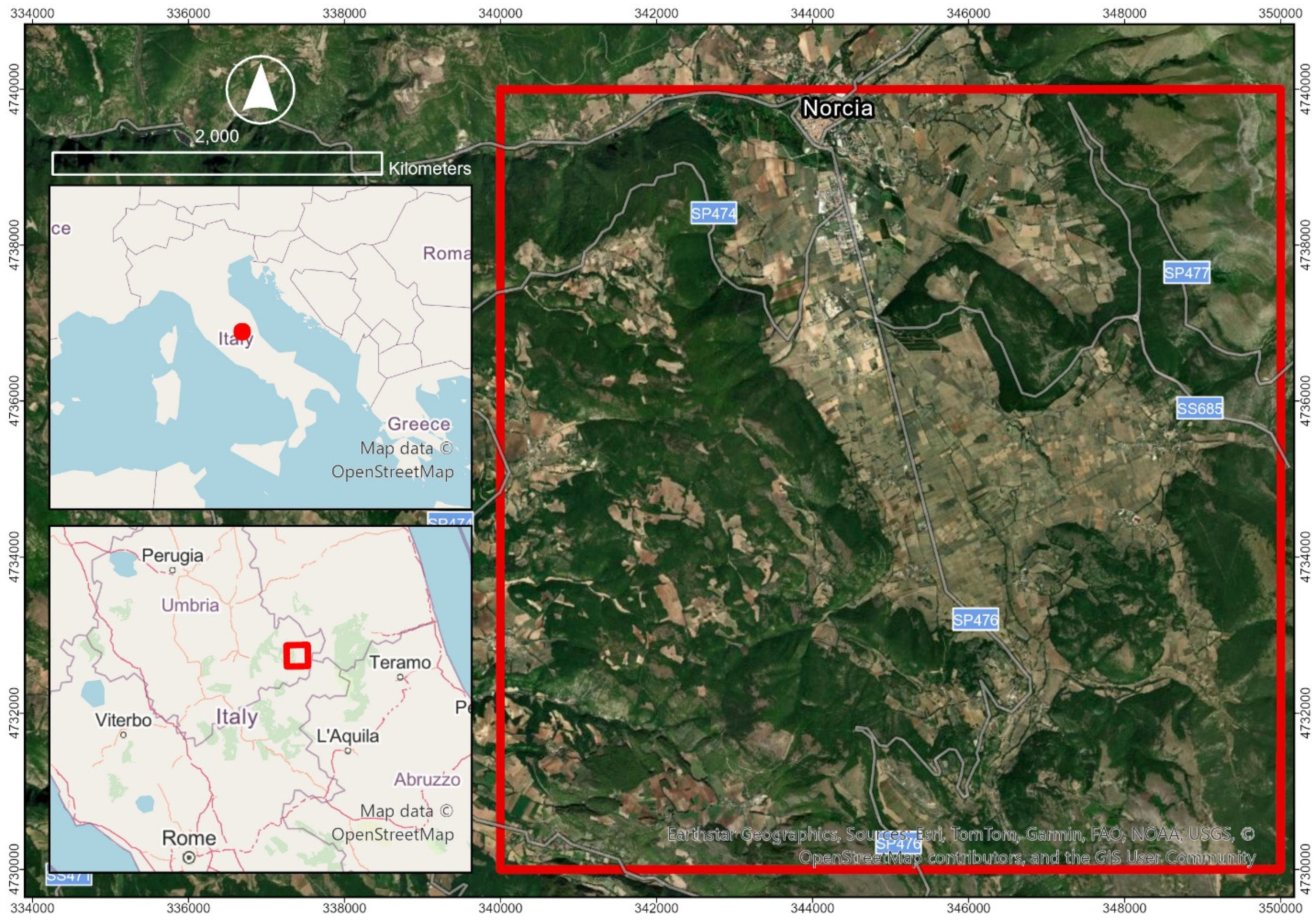
The study area covers 100 square kilometers near Norcia, in Perugia Province, Umbria, Italy (Figure 1). The region’s morphology is complex, encompassing the tectonically formed plateau of Santa Scolastica, which is situated at the heart of the Umbria-Marche Apennines and included within the Sibillini Mountains National Park. Hence, the area’s landscape is shaped by the convergence of mountainous terrain and the enduring presence of cultivable land and extensive pastures. The area is situated at an elevation between 561 and 1692 m above sea level, with a mean altitude of 930 m. As a result of its historical collective use, the agrarian landscape is configured into a distinctive open-field system. The region is distinguished by the cultivation of lentils, which were designated a Protected Geographical Indication in 1999.

2.2. Data Provided by AGEA

Land Parcel Identification Systems (LPISs), as geodatabases for identifying and monitoring land parcels to manage agricultural subsidies, are characterized by technical specifications that vary from one MS to another, as various types of reference parcel exist. The statement of Art 6.1 of the Commission Reg. No. 796/2004 [3] allows four types of representation of reference parcels: cadastral parcel, agricultural parcel, farmers’ block and physical block. Member States that base their LPIS model on the ownership declared by land registers adopt the cadastral parcel model; this model is utilized in Italy [13]. Consequently, the cadastral dataset provided to AGEA by the Italian Tax Agency (AE—Agenzia delle Entrate) was used to create reference parcel boundaries over the test area.

Additionally, the orthophoto acquired in June 2023 by AGEA served as the reference scene over the test area. Indeed, among its mandates, AGEA is also responsible for conducting an aerial photogrammetric survey over the whole national land area, conducted both in visible and near infrared ranges, with an average ground sampling distance (GSD) of 20 cm. Subsequently, AGEA is also responsible for the processing of such data to produce RGBNIR orthophotos at a scale of 1:5000, with a pixel resolution of 20 cm [14].

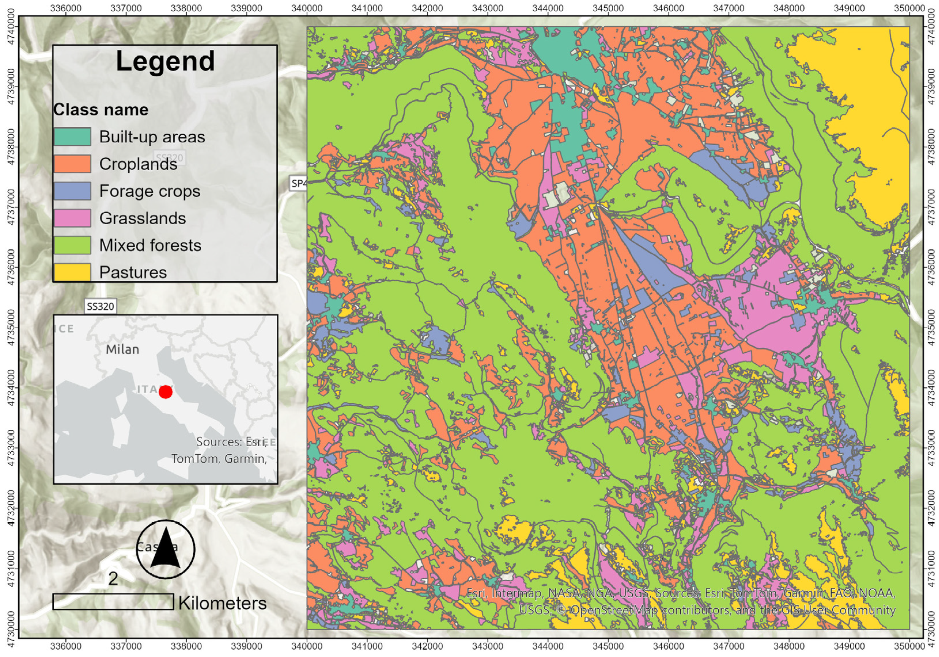
Finally, the land-cover map generated annually by AGEA from its ortho-imagery was used as a land-cover reference for the study. As shown in Figure 2, the predominant land-cover types within the region are mixed forests (52.6%), croplands (19.6%), pastures (9.6%), grasslands (7.4%), built-up areas (3.5%), and forage crops (3.4%).

2.3. PlanetScope Data

PlanetScope (PS) is an optical satellite imaging mission owned and managed by the private company Planet Labs. The constellation is composed of almost 130 platforms, which acquire imagery of the Earth’s entire land surface on a daily basis. The PlanetScope spectral resolution spans a range between 431 and 885 nm, comprising eight different bands (

Table 1. PlanetScope’s spectral bands and their respective wavelength ranges.

Spectral Bands	Wavelength Range
Coastal Blue	431–452
Blue	465–515
Green I	513–549
Green II	547–583
Yellow	600–620
Red	650–680
Red-Edge	697–713
NIR	845–885

). The current sensor, PSB.SD (Super-Dove), is the same that was used to acquire the dataset used for this study [15].

The PlanetScope imagery employed in the current study was the analytic Surface Reflectance (SR) ortho scene product, in which surface-reflectance values are scaled by 10,000 [15]. Additionally, these are orthorectified and projected into a cartographic spatial reference system (UTM). The resulting spatial resolution is three meters.

The dataset, which was released by Planet Labs for the study, consists of 59 images that were acquired for twenty-five different dates between 7 March and 7 October 2023 over the test area. The images were collected at an average interval of one every eight days, with significant variability. The minimum interval between two acquisitions was two days, while the maximum was twenty-three days. The standard deviation of the acquisition intervals was determined to be six days. It is important to note that the frequency of acquisitions was contingent upon atmospheric conditions, which served to restrict the selection to images characterized by minimal cloud coverage. Indeed, the mean cloud-coverage rate across the entire image set was estimated to be 0.1%, with a maximum observed value of 0.87%. Refer to

Table 2. PlanetScope acquisition dates.

Month	Dates
March	7; 16; 23; 30
April	7; 27
May	5; 29
June	2; 21; 27
July	7; 12; 17; 22
August	1; 8; 14; 18; 27
September	1; 4; 27
October	1; 7

for a comprehensive list of all PlanetScope acquisition dates.

2.4. Extraction of Land Parcels

The aim of this study is to delineate a procedure to exploit the high temporal and geometric resolution of PlanetScope data to extract agricultural parcels. A processing chain comprising three steps was developed, with the aim of leveraging the temporal variable. These steps include:

• Mosaicking and color correction of PlanetScope imagery to generate a homogeneous time series.
• Calculation of the Normalized difference Vegetation Index (NDVI) for the whole time series.
• Image segmentation for extraction of agricultural parcels.

2.4.1. Mosaicking and Color Correction

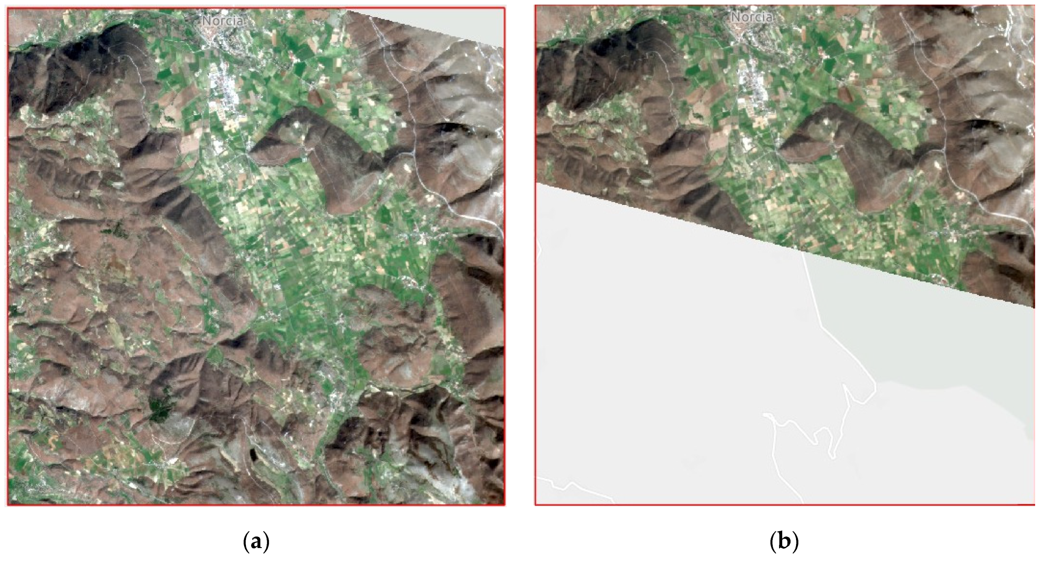
Only the scenes acquired on 29 May and 7 July captured the entire study area; all the other dates included two or more images, meaning that more than one image was acquired on the same date. The aim of the mosaicking step was to make the dataset homogeneous, modeling it through the rule “one image per date”, to obtain a comprehensive set of twenty-five images, each referring to only one acquisition date. In instances in which the mosaicking of two images was necessary to ensure comprehensive coverage of the test area, the raster pairs were mosaicked using the workflow proposed by Seamless Mosaic, a tool available within the software ENVI (6.1 version). For each pair, the reference and the adjusted scenes were selected on the basis of their dimensions: the largest scene was used as the reference scene, while the smallest scene was used as the adjusted scene (Figure 3).

Consequently, the reference scene was layered on top of the mosaic. Then, the image footprints of both the reference and the adjusted images were clearly delineated in order to compute which portion of the adjusted scene would fill the empty portion of the reference scene. The color-correction process was then applied to each mosaic. This algorithm maps discrete greyscale levels from the histogram of the adjusted scene to the corresponding greyscale levels in the reference scenes, considering only the area where the two images overlap. The procedure subsequently interpolates the statistics of the two image histograms, and the resulting matching algorithm is applied to the area of the adjusted image where the reference does not overlap. This approach minimized any radiometric artefacts resulting from the mosaicking. The resultant dataset consisted of twenty-five images, with each image corresponding to a specific date (for a complete list of the resulting image IDs, refer to

Table 3. Scene ID, acquisition date and file name of each of the 25 scenes composing the dataset. The scenes captured by single images are highlighted in green, while the scenes generated by the mosaicking of two images are highlighted in orange.

ID	Acquisition Date	File Name
1	03/07/2023	20230307_090404_47_24b2_3B_AnalyticMS_SR_8b_clip
2	03/16/2023	20230316_085941_53_2430_3B_AnalyticMS_SR_8b_clip
3	03/23/2023	20230323_093937_17_227b_3B_AnalyticMS_SR_8b_clip
4	03/30/2023	20230330_090739_19_24be_3B_AnalyticMS_SR_8b_clip
5	04/07/2023	20230407_090308_37_2465_3B_AnalyticMS_SR_8b_clip
6	04/27/2023	20230427_093907_91_2482_3B_AnalyticMS_SR_8b_clip
7	05/05/2023	20230505_093834_78_2479_3B_AnalyticMS_SR_8b_clip
8	05/29/2023	20230529_090833_53_24b9_3B_AnalyticMS_SR_8b_clip
9	06/02/2023	20230602_090648_56_24b4_3B_AnalyticMS_SR_8b_clip
10	06/21/2023	20230621_090410_77_24b6_3B_AnalyticMS_SR_8b_clip
11	06/27/2023	20230627_090521_83_24cc_3B_AnalyticMS_SR_8b_clip
12	07/07/2023	20230707_090259_46_241f_3B_AnalyticMS_SR_8b_clip
13	07/12/2023	20230712_094459_06_247a_3B_AnalyticMS_SR_8b_clip
14	07/17/2023	20230717_093941_43_2488_3B_AnalyticMS_8b_meta_SR
15	07/22/2023	20230722_094258_28_2446_3B_AnalyticMS_SR_8b_clip
16	08/01/2023	20230801_090504_54_24c4_3B_AnalyticMS_SR_8b_clip
17	08/08/2023	20230808_090845_82_2427_3B_AnalyticMS_SR_8b_clip
18	08/14/2023	20230814_094652_88_2479_3B_AnalyticMS_SR_8b_clip
19	08/18/2023	20230818_090719_99_2430_3B_AnalyticMS_SR_8b_clip
20	08/27/2023	20230827_090503_52_24b9_3B_AnalyticMS_SR_8b_clip
21	09/01/2023	20230901_094748_28_241c_3B_AnalyticMS_SR_8b_clip
22	09/12/2023	20230912_094456_48_241c_3B_AnalyticMS_SR_8b_clip
23	09/27/2023	20230927_094829_09_2473_3B_AnalyticMS_SR_8b_clip
24	10/01/2023	20231001_094607_35_2498_3B_AnalyticMS_SR_8b_clip
25	10/07/2023	20231007_094527_73_2473_3B_AnalyticMS_SR_8b_clip

).

2.4.2. NDVI Calculation

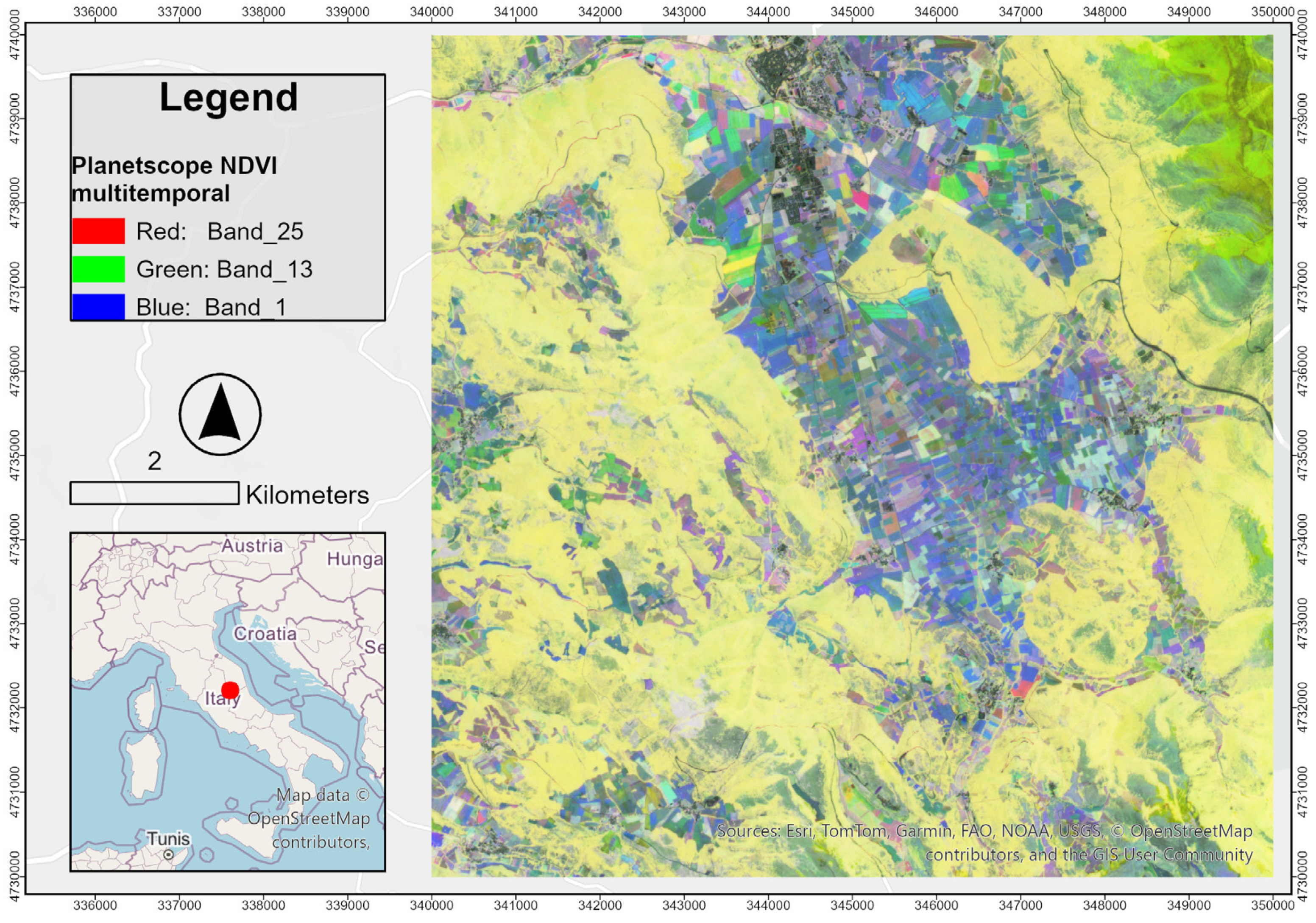
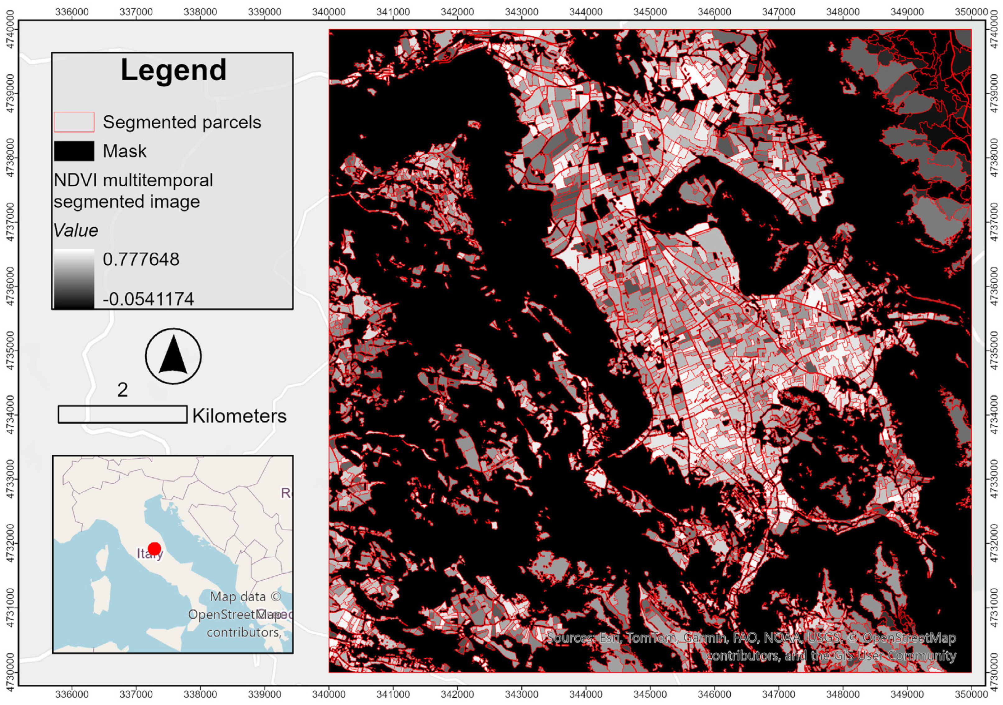
In this step, the NDVI map was computed for each scene. Then, the resulting twenty-five NDVI images were stacked into a new multiband raster (Figure 4), in which each band refers to a single acquisition date.

2.4.3. Image Segmentation

In the context of increasing demand for methods capable of extracting value-added information from geospatial data, object-based image analysis (OBIA) is a framework dedicated to dividing remote sensing imagery into meaningful image objects (or segments), rather than individual pixels [16]. Traditionally, OBIA includes two principal steps, image segmentation and object classification. Image segmentation refers to the partitioning of an image into spatially adjoining and homogenous regions (the segments), comprising the foundation for further analysis [17]. Therefore, segmentation algorithms aim at clustering neighboring pixels into objects that should ideally correspond to real-world features.

As LPIS is a geodatabase designed for identifying and monitoring land parcels to manage agricultural subsidies, the ability to accurately extract parcel boundaries is a primary requirement. In this study, image segmentation serves as a fundamental step in assessing the potential of LPIS parcel-boundary extraction using PlanetScope data. Since agricultural parcels typically exhibit well-defined radiometric borders and homogeneous content, the segmentation of the multitemporal NDVI dataset was performed using the Edge method, which is particularly well-suited for identifying features with distinct boundaries and uniform internal texture [18]. The algorithm was implemented through an established workflow available in ENVI 6.1 named Segment Only Feature Extraction. It comprises the following steps:

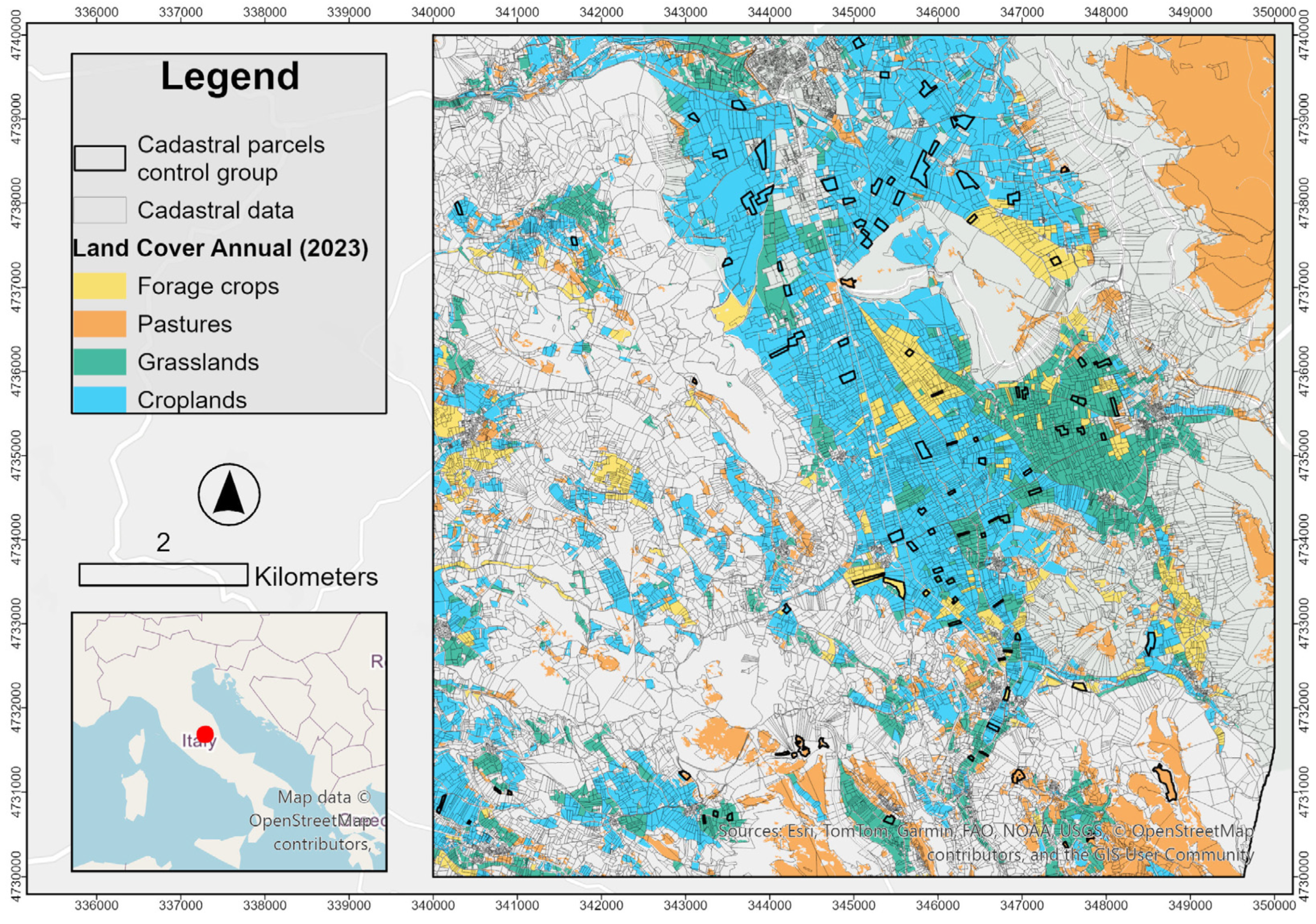
• Creation and application of an input mask to filter out from the scene all the coverage classes not relevant for extraction of agricultural parcels. Among the land-cover classes provided in Land Cover Annual (2023), only surfaces covered by the classes Croplands, Grasslands, Forage Crops, and Pastures were considered for further analysis.
• Per-band gradient computation. Application of the Sobel filter with a kernel size of 3 × 3 to generate twenty-five gradient images from the PlanetScope NDVI multitemporal image set. The Sobel filter is an edge-detection method that maps the magnitude of local changes (the contrast) in the pixel values of an image [19]. Globally, these changes are measured by a gradient image, in which higher pixel values represent areas with higher pixel contrast.
• Fusion of per-band gradients. The resulting set of twenty-five gradient images is fused into a single gradient image. As outlined in U.S. Patent No. 8,260,048 B2—which underpins the Segment Only Feature Extraction workflow implemented in ENVI 6.1—the fusion method MAX is used to perform this operation. This method selects, for each pixel location, the maximum value of gradient values across all bands. The MAX fusion approach effectively emphasizes the most salient spatial transitions present in any gradient images, closely matching the way humans perceive object boundaries [18].
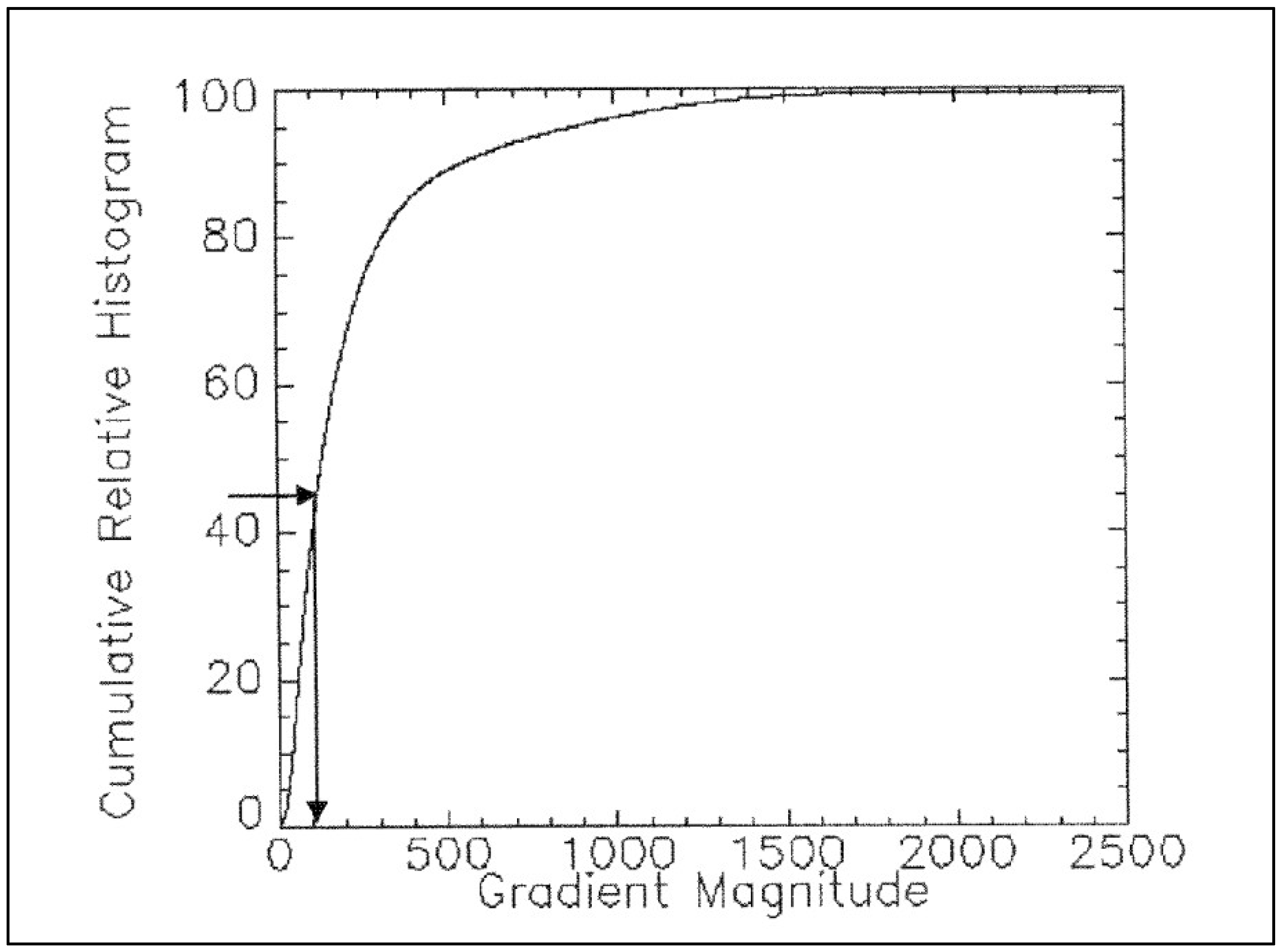
• Computation and normalization of the cumulative relative histogram (CRH) of the gradient values (Figure 5).
• Setting of scale-level threshold to filter the gradient image. Pixels in the gradient image with values lower than a selected cumulative relative histogram threshold (scale level) are replaced with the threshold value.

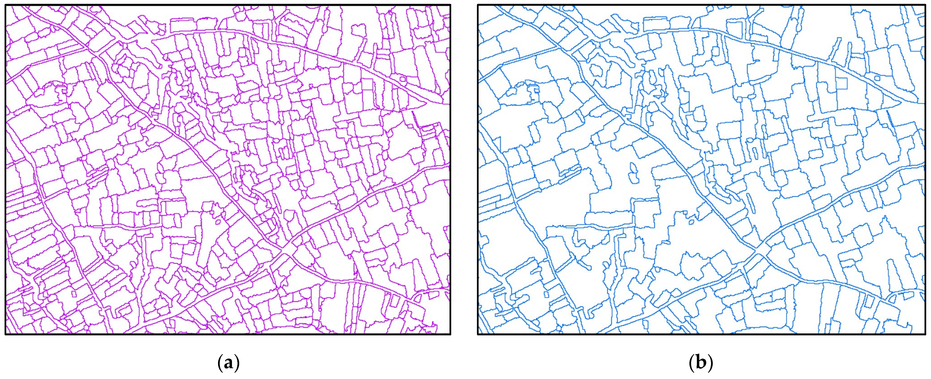
Therefore, the application of the scale level modifies the gradient image, discarding from it the values in percentiles that fall below the specified threshold and discarding the areas with pixel contrast lower than a defined threshold. This process allows for control of the degree of over or under-segmentation produced by the algorithm. Undersegmentation occurs when image segmentation fails to define individual objects, thus constructing a single object that may contain multiple features. By contrast, oversegmentation error occurs when unnecessary boundaries are delimited such that multiple contiguous objects potentially belonging to the same features are formed. Generally, increasing the scale level results in the retention of objects that exhibit the most distinct edges. In the present case, scale levels of 10%, 20%, 30% (Figure 6), and 40% were separately selected to generate different segmentation results.

6.

Segmentation of the modified gradient image through the Watershed Transform. This method is used to generate separate segments based on the concept of hydrologic watersheds [20]. In this framework, the lower the value of the pixel gradient, the lower its elevation; this type of pixel is called a minimum. The watershed algorithm sorts pixels by increasing gradient value, then floods the image starting with the lowest gradient values (the uniform part of the objects) and proceeding to the highest gradient values (the edges), partitioning the image into segments (regions with similar pixel intensities) based on the computed watersheds. The result is a segmentation image in which each region is assigned the mean spectral values of all the pixels that belong to that region.

7.

Merging of the segmentation image to further refine and correct tendencies to over or undersegmentation. In this step, a Full Lambda Schedule algorithm was applied. This method involves the computation of the mean spectral values, areas, and lengths of common boundaries of a pair of adjacent segments. Then. it computes the Euclidian distance among those attributes for each possible segment pair and merges the objects if their similarity exceeds a defined threshold value [21]. In the present case, due to the observed broad tendency of the dataset to generate oversegmentation errors, the merge level was set to 97.5% to resolve the issue (four different scale levels (10%, 20%, 30%, 40%), each combined with a merge level of 97.5%, were selected through visual interpretation as the preferable solutions for delineating agricultural parcels as accurately as possible compared to the cadastral dataset).

The resulting four segmentation images were converted into segmentation vectors. Figure 7 shows the segmentation differences created by varying the scale level from 10% to 40%.

2.5. Assessment of Segmentation Accuracy

Multiple methods exist to assess the accuracy of segmentation. segmentation errors can be identified through visual inspection, but it is time consuming, especially when assessing large areas and comparing numerous segmentation outputs. Additionally, visual interpretation is subjective, as the results produced by the same or different operators may not be reproducible. On the other hand, several quantitative methods for assessing the quality of image segmentation exist and grouped into two main categories: supervised and unsupervised methods [22]. Supervised methods essentially compare segmentation output to a reference dataset and measure the similarity or discrepancy between the two representations. Ideally, there should be a one-to-one correspondence between the reference objects and segments. In turn, supervised methods can be divided into two main categories: geometric and non-geometric. Geometric methods rely on quantitative metrics that describe geometric and topologic similarities between reference objects and segments [23]. Non-geometric methods essentially leverage the similarity in the content of the objects, considering, for instance, their spectral values [24] or topographic parameters (e.g., slopes, curvatures) [25]. Finally, unsupervised methods measure some desirable properties of the segmentation outputs (e.g., an object’s spectral homogeneity) without comparing them with a reference, thus measuring their quality [26].

In the present study, a supervised geometric method was selected to assess the accuracy of the four segmented parcel maps derived from the use of four different scale-level thresholds. It involved the following steps:

• Sampling of 100 reference parcels (ground truth) from the cadastral dataset provided by the Italian Tax Agency (AE).
• Selection of 100 corresponding segmented parcels from each of the segmented parcel sets.
• Definition, at the local level, of geometric metrics to compare reference and segmented parcels.
• Definition, at the global level, of the accuracy of each segmented parcel set.

2.5.1. Sampling of Reference Parcels

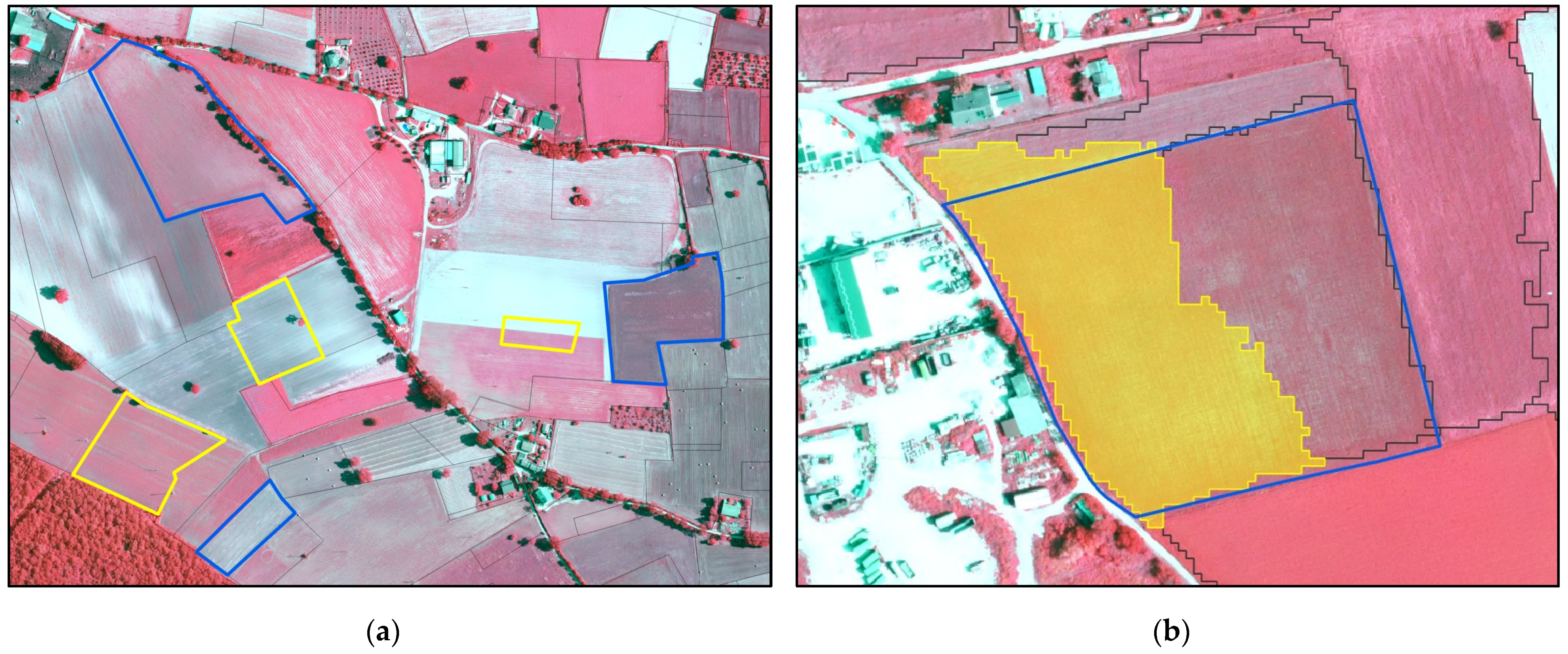
In this step, a sample of 100 parcels was selected as ground truth from the set of cadastral parcels provided by AE. First, it was necessary to ensure that the centroid of each reference parcel fell within the boundaries of the land-cover class considered during the segmentation process (Croplands, Grasslands, Forage Crops, and Pastures) (Figure 8). Secondly, reference parcels were selected by means of photointerpretation by superimposing the cadastral dataset over the 20 cm-orthophoto provided by AGEA, which was displayed as a false-color composite to enhance vegetation features. This step ensured the selection of only those parcels that were effectively extant in 2023 and that were delineated by well-recognizable radiometric borders (Figure 9a). Despite the time-consuming nature of this stage, it ensured the quality of the reference parcels used as ground truth to test the accuracy of the segmentation. It is important to note that the sampling was conducted to maintain the initial proportion of parcels belonging to each cover type; thus, the sampling included forty-eight parcels belonging to the class Cropland; twenty-seven belonging to the class Grasslands; fourteen belonging to the class Pastures; and belonging eleven to the class Forage Crops.

2.5.2. Selection of the Corresponding Segments

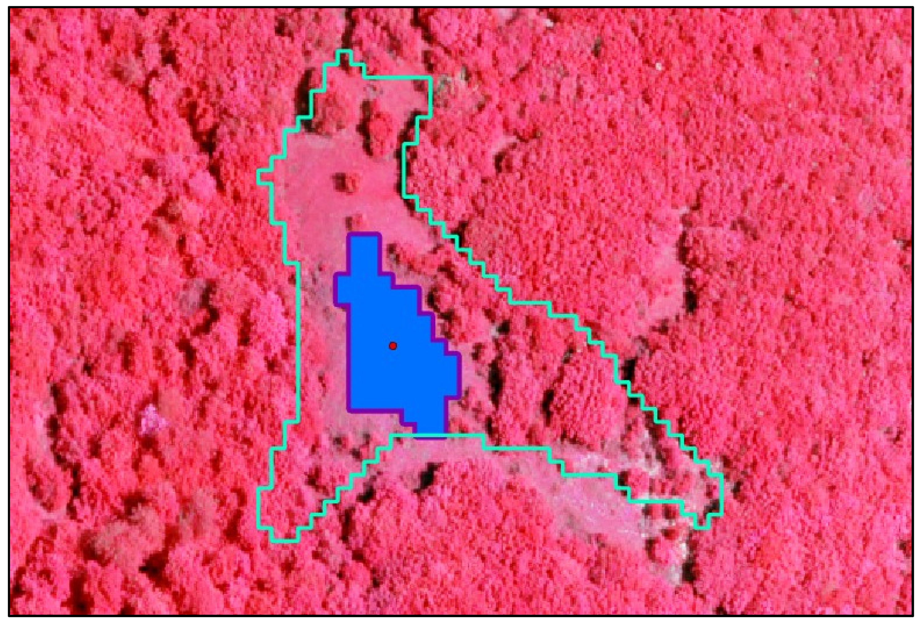
In this step, a total of 100 segments were selected from each of the parcel sets derived from the application of the four scale-level thresholds. The segmented parcels were first selected on the basis of their topological intersection with the 100 reference parcels. This resulted in a set of segmented parcels with a many-to-one relation to the set of reference parcels. Consequently, the one-to-one relationship between the two ensembles was accomplished by manually selecting only the segmented parcel exhibiting the highest degree of overlap with each corresponding reference parcel (Figure 9b).

2.5.3. Local Definition of Accuracy

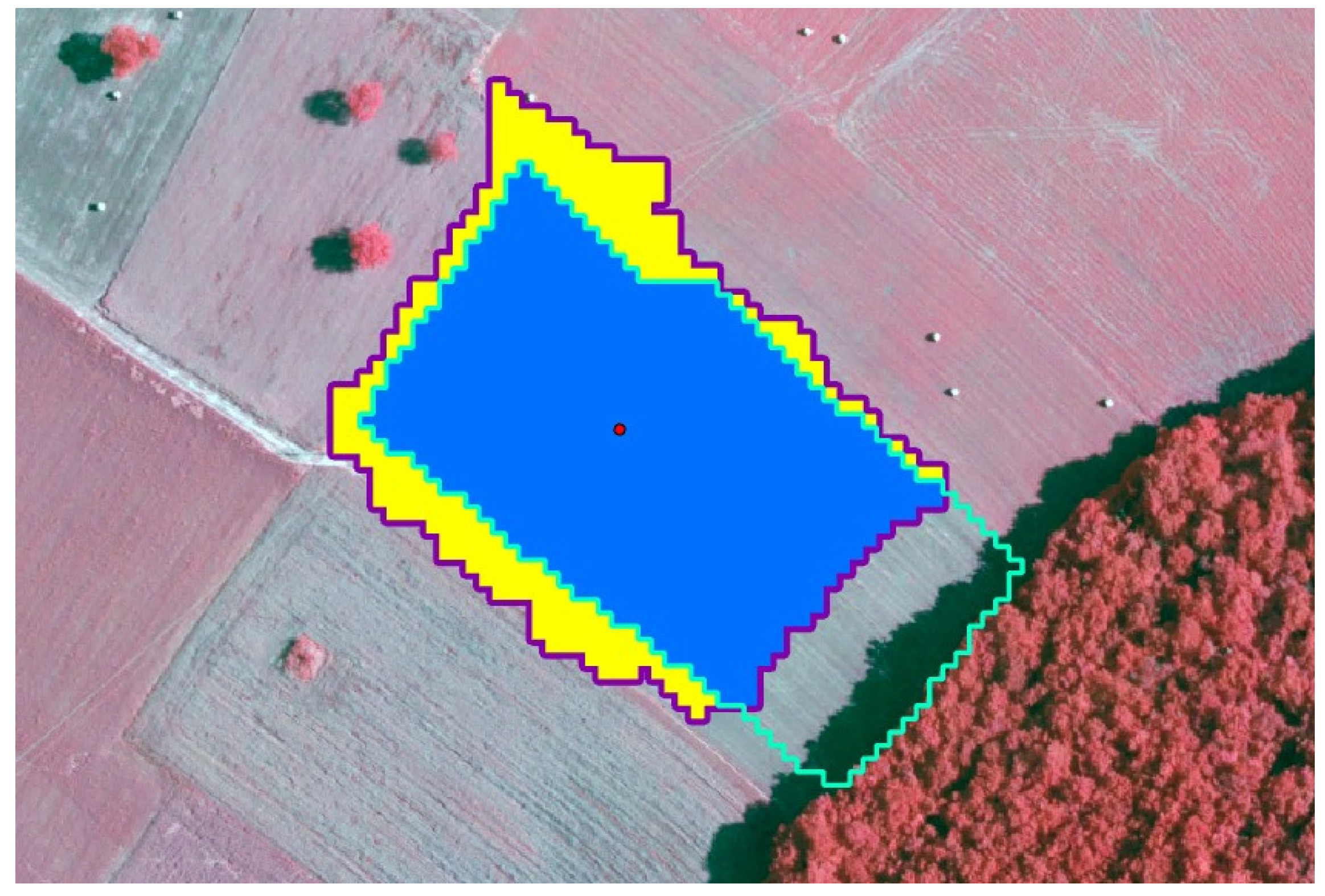
Following the establishment of the one-to-one relationship between the two parcel groups, three local metrics of similarity were computed based on the relationship between the areas of reference and the segmented parcels. First, the metric overlapping area rate (OlpAR) was determined by calculating the ratio of the overlapping area between each segment (S) and its reference parcel (R) to the total reference parcel area:

$$OlpARi={\displaystyle \frac{A(Si \cap Ri)}{A\left(Ri\right)}}$$

(1)

Subsequently, the metric overflowing area rate (OflAR) was determined by calculating the ratio of the segment area overflowing the boundaries of its reference to its total area (Figure 10):

$$OflARi={\displaystyle \frac{A(Si \cap Ri)}{A\left(Si\right)}}$$

(2)

Subsequently, each overflowing area rate was subtracted from the corresponding overlapping area rate. Indeed, the ideal total correspondence is defined as a 100% of the overlapping area rate between the segment and its reference, with a 0% overflowing area rate outside the boundaries of the reference. The result, which potentially ranges between −100% and +100%, was then normalized to a positive range of 0–100% to define the local overall accuracy (LOA):

$$LOAi={\displaystyle \frac{\left[\right(OlpARi-OflARi+1)}{2}}\times 100$$

(3)

Concurrently, the photointerpretation of each case determined that an 80% local overall accuracy threshold generally represented the minimum required to observe correctly delineated segmentation parcels.

Finally, a third local metric named area difference (AD) was calculated to complement the local overall accuracy with additional information: the difference between each segment’s area and that of the corresponding reference.

$$\mathrm{A}\mathrm{D}i=\mathrm{A}\left(\mathrm{S}i\right)-\mathrm{A}\left(\mathrm{R}i\right)$$

(4)

This subtraction resulted in a binary evaluation: positive values indicated that segmented areas were larger than reference areas, thus indicating undersegmentation errors in cases in which local overall accuracy was below 80%. Conversely, negative values, indicating segmented areas smaller than reference areas, served as a proxy for oversegmentation errors with the same accuracy threshold.

2.5.4. Global Definition of Accuracy

The accuracy of the four segmented parcel sets, resulting from the use of four different scale thresholds, was determined globally by averaging the 100 local overall accuracy rates, weighted by the respective segment areas. It resulted in a global accuracy metric named the mean weighted accuracy rate (MWAR), as follows:

$$MWAR={\displaystyle \frac{{\sum }_{i=1}N=1 LOAi\times A\left(Si\right)}{{\sum }_{i=1}N=1 A\left(Si\right)}}$$

(5)

The same process was applied to the overlapping and overflowing area rates, which were averaged and weighted for each segment’s area. The results are two further global metrics: mean weighted overlapping rate and mean weighted overflowing rate.

$$MWOlpAR={\displaystyle \frac{{\sum }_{i=1}N=1 OlpARi\times A\left(Si\right)}{{\sum }_{i=1}N=1 A\left(Si\right)}}$$

(6)

$$MWOflAR={\displaystyle \frac{{\sum }_{i=1}N=1 OflARi\times A\left(Si\right)}{{\sum }_{i=1}N=1 A\left(Si\right)}}$$

(7)

Finally, by counting on the basis of their sign each local area difference related to parcels extracted with a local overall accuracy lower than 80%, it was possible to compute the undersegmentation error rate (number of local-area differences with positive signs) and its complement, the oversegmentation error rate (number of local-area differences with negative signs), for each segmented parcel sets.

3. Results

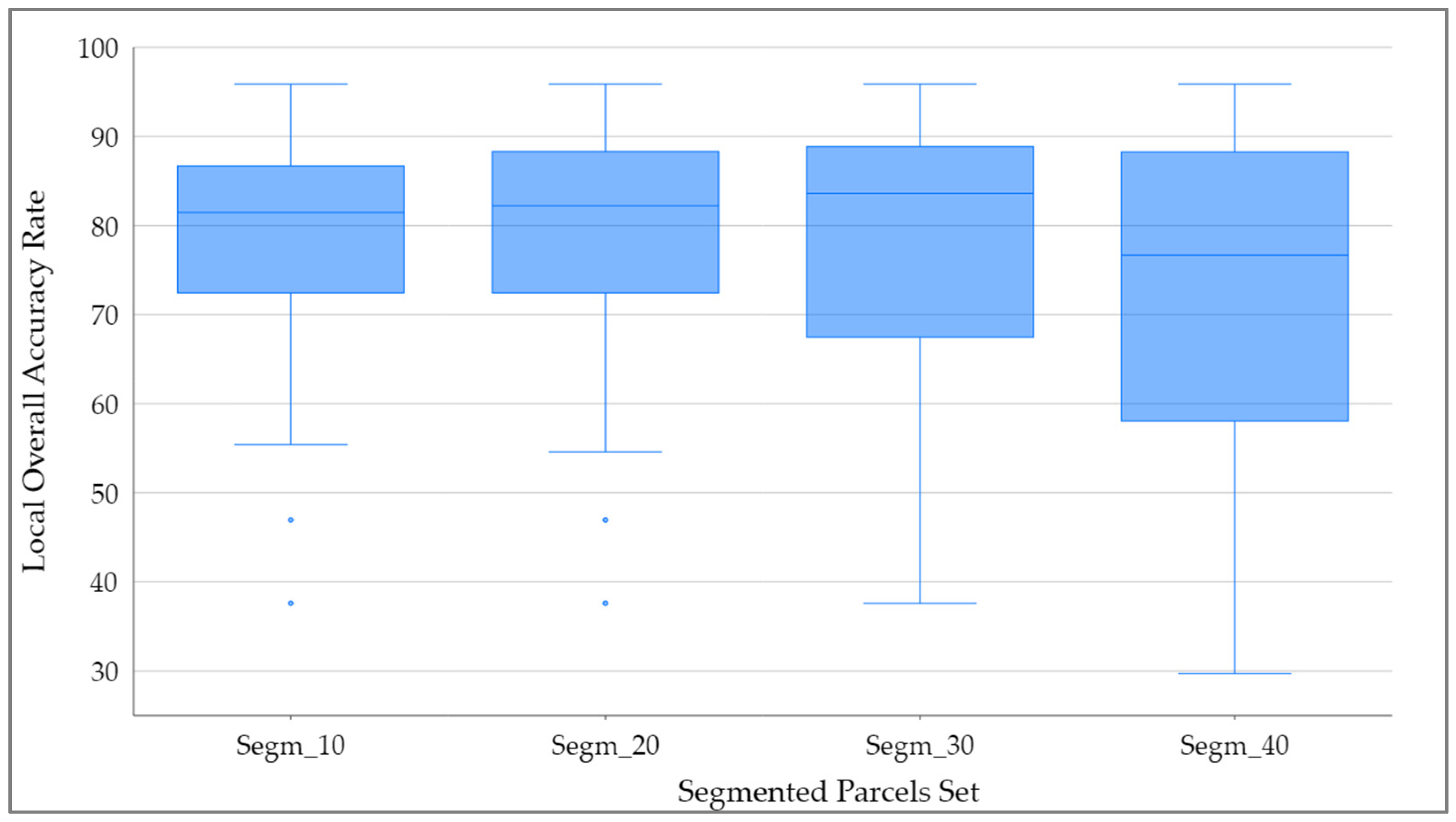
The study found that segmentation on NDVI images from PlanetScope, tested at four different scales, achieved satisfactory accuracy. The analysis revealed that the mean weighted accuracy rate exhibited a range of values between 79% and 83% in all four cases. Specifically, the segmented parcel set obtained with the scale level set to 30% (hereafter referred to as Segm_30) achieved the highest mean weighted accuracy rate, at 83.33%. The output when the scale was set to 20% (Segm_20), the mean weighted accuracy rate was 81.93%, while when the scales were set to 10% (Segm_10) and 40% (Segm_40), the mean weighted accuracy rates were 81.06% and 79.33%, respectively. The maximum local overall accuracy value was 96% for all four outputs. These findings, along with the statistical parameters of the local overall accuracy distribution for each segmented parcel set, are summarized in

Table 4. Local overall accuracy values associated with the four scale levels.

Segmented Parcels Set	Mean Weighted Overall Local Accuracy Rate (%)	Overall Local Accuracy Rate—Min (%)	Overall Local Accuracy Rate—First Quartile (%)	Overall Local Accuracy Rate—Median (%)	Overall Local Accuracy Rate—Third Quartile (%)	Overall Local Accuracy—Max (%)
Segm_10	81.06	37.59	72.44	81.48	86.70	95.87
Segm_20	81.93	37.59	72.44	82.22	88.31	95.87
Segm_30	83.33	37.59	67.45	83.60	88.84	95.87
Segm_40	79.33	29.68	58.06	76.68	88.27	95.87

.

The statistical distribution of the entire set of 100 local overall accuracy values for each segmented parcel set was examined (Figure 11), revealing that the minimum local overall accuracy values ranged from 29% (Segm_40) to 37% (for Segm_10, Segm_20, and Segm_30).

Additionally, the mean weighted accuracy rate was associated with its two constituent parameters: the mean weighted overlapping rate and the mean weighted overflowing rate. From the analysis of their trends with respect to the scale levels, it appears evident that global accuracy exhibits a non-linear correlation with increasing scale level. As shown in

Table 5. Mean weighted accuracy rate, mean weighted overlapping rate, mean weighted overflowing rate, and mean area of the segmented parcels for the four scales.

Segmented Parcels Set	Mean Weighted Accuracy Rate (%)	Mean Weighted Overlapping Rate (%)	Mean Weighted Overflow Rate (%)	Segmented Parcels Mean Area 1 (m2)
Segm_10	81.06	84.23	24.46	7308.54
Segm_20	81.93	87.17	28.46	8054.82
Segm_30	83.33	89.25	36.68	9343.62
Segm_40	79.33	92.48	63.29	17,894.56

¹ The reference parcels mean area is equal to 7017.93 m².

, an increase in scale level from 10% to 30% increases the accuracy from 81.06% to 83.33%. Conversely, a further escalation in scale level to 40% caused the mean weighted accuracy rate to decline to 79.33%.

This phenomenon can be attributed to the increase in both overlapping and overflowing rates observed as the scale level increases. Indeed, while the overlapping rate contributes positively to segmentation accuracy, the overflow rate has a negative impact. In this particular instance, a scale level of 30% represents the optimal balance between achieving the maximum overlapping rate and minimizing the overflowing rate.

Subsequently, by analyzing the local values obtained from the area difference metric, the number of inaccurately segmented parcels and the predominant error type among them were determined. The results are summarized in

Table 6. Inaccurately segmented parcels (local overall accuracy < 80%) and the predominant error type affecting them, represented as a percentage.

Segmented Parcels Set	N. of Inaccurately Segmented Parcels	Segmentation Error Rate
Segm_10	46/54	50%—under-segmentation
Segm_20	43/57	65.12%—under-segmentation
Segm_30	42/58	66.66%—under-segmentation
Segm_40	58/42	82.75%—under-segmentation

.

The undersegmentation error rate, which was obtained by normalizing the number of positive area-difference values (i.e., instances in which the segmented areas were larger than the reference areas), exhibited an increase that was correlated with the increase in scale level. This phenomenon was most pronounced among the two sets of segments obtained by using the highest and lowest scale values (i.e., Segm_10 and Segm_40). Conversely, the undersegmentation error rate showed minimal sensitivity to the increase in scale level from 20% to 30%, with rates of 65.12% and 66.66% observed in subsets of 43 and 42 segments, respectively. The combinations of scale levels and merge levels selected for the survey did not result in oversegmentation errors, except in Segm_10, which exhibited a perfect balance between under- and oversegmentation.

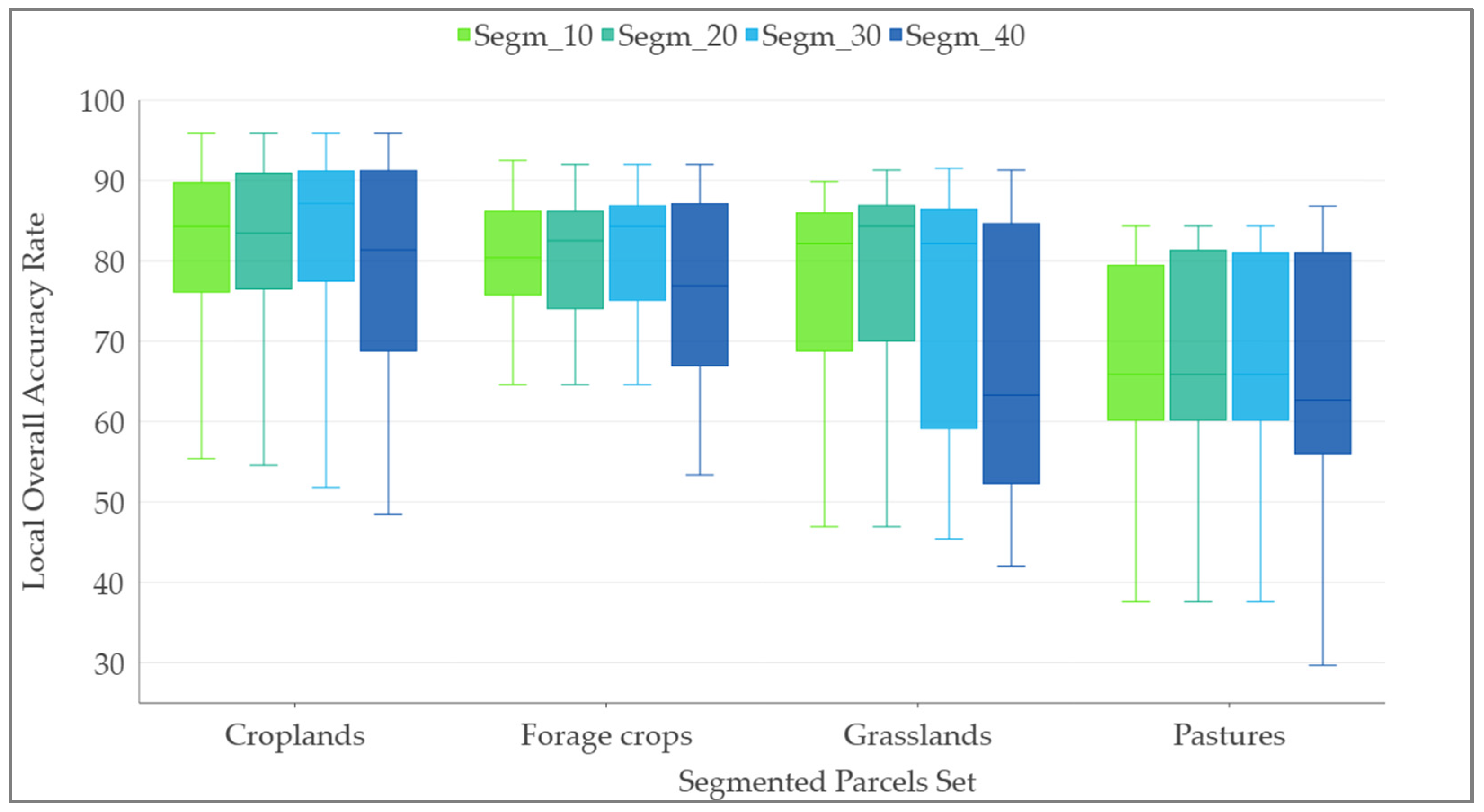
Finally, the local overall accuracy values were examined by land-cover classes and divided into segmented parcel sets to elucidate possible segmentation issues linked to the spectral content of land coverages (Figure 12). This analysis demonstrated that all segmented parcel sets in the class Pastures have lower local overall accuracy in minimum, maximum and mean values. Segments in class Forage crops produced the most stable results, with low variability and relatively high minimum values. Conversely, segments classified as croplands exhibited the highest median and maximum values, although the minimum values were notably low.

While it was challenging to identify a consistent pattern for parcels in the Croplands and Forage Crops classes, the reference parcels within the Pastures class demonstrated that the cadastral information frequently lacked precision in accurately representing the current state of the land. This discrepancy between cadastral information and the updated condition of pastures, which frequently includes tree cover or indistinct boundaries (Figure 13), introduces greater uncertainty to the segmentation results for parcels classified within this category.

4. Discussion

The segmentation of PlanetScope data for the purpose of enhancing LPIS updates and maintenance has demonstrated significant potential. The stack of twenty-five NDVI images with a geometric resolution of 3 m and a dense temporal component provided valuable data for land-parcel delineation. A key finding of this study is that the edge-based segmentation method, when applied to multitemporal PlanetScope imagery, effectively extracts parcel boundaries with an acceptable level of accuracy, despite the discrepancy in geometric resolution between PlanetScope data (3 m) and the traditional aerial orthophotos employed by AGEA (20 cm) for the same purpose. These findings align with the results of previous studies demonstrating the utility of multitemporal optical data for agricultural monitoring [10,11,12].

The geometric, supervised method employed to assess the segmentation accuracy highlights that when the PlanetScope multitemporal NDVI dataset was segmented into four different scale levels (10%, 20%, 30%, 40%), the mean weighted accuracy rates ranged from 79.33% to 83.33%, with the highest accuracy recorded at a 30% scale level. This evaluation method takes into account the areal relationship between reference and segmented parcel areas. Although this approach has been widely discussed in the literature [23,27], this study enhances segmentation evaluation by integrating the two key metrics—overflowing area rate and overlapping area rate—that influence segmentation accuracy in opposite ways, along with the sign of the area difference. This integration enables the identification of error types in cases of low accuracy, which is essential for recalibrating the segmentation algorithm and enhancing its overall performance.

The major strength of this approach is the incorporation of temporal resolution as a crucial factor for parcel delineation. The results suggest that the availability of the temporal dimension can compensate for spatial resolutions lower than those of traditional orthophotos. The incorporation of the temporal path of vegetation indices enables the consideration of the phenological cycles of vegetation coverage within the parcels, enabling a more comprehensive and reliable delineation of their boundaries. This appears to fully justify a shift from a static LPIS paradigm, which is based on mono-temporal data, to a dynamic LPIS paradigm based on multi-temporal analysis. A further strength of the survey lies in investigating segmentation and refining quantitative methodologies for assessing segmentation accuracy. Indeed, such assessment is commonly undertaken by means of qualitative methods or regarded as a preliminary step in object-based image analysis (OBIA). However, frequently, these types of analyses only assess the accuracy of segment classification, rather than evaluate the segmentation step itself [17]. A third strength of the study is the comparative approach across different scales, which enables a critical examination of the segmentation algorithm, improving our understanding of its functioning and its impact on result quality.

A primary limit of the research pertains to the prevailing reliance on visual interpretation and manual intervention for the establishment of the one-to-one correspondence between segmented and reference parcels. The full automation of this task is particularly challenging due to the difficulty of parametrizing the wide variety of conditions required to accurately determine which segment best corresponds to the reference. Another limitation is the adoption of only a geometric method to evaluate segmentation accuracy. Despite the area-based procedure having been demonstrated to generate satisfactory descriptions and rankings of segmentation accuracy on a case-by-case basis, the integration of supplementary non-geometric methods, such as segment spectral and texture attributes, into multivariate analyses would allow a more comprehensive evaluation, thereby enhancing the robustness of the method for accuracy assessment. A third limitation consists of the underexploitation of PlanetScope’s spectral resolution, since the study used only the red and NIR bands to calculate the Normalized Difference Vegetation Index (NDVI). A fourth limitation of the study lies in the exclusive use of the local overall accuracy metric, which is inherently area-based. This metric was deliberately selected to align with the operational priorities of LPIS maintenance, where the principal objective is to determine the eligibility of agricultural surface areas, rather than to attain submeter accuracy in delineating parcel boundaries. Although vector-based accuracy assessment methods—such as those relying on boundary displacement—are valuable tools for evaluating the geometric precision of parcel outlines, they were not implemented in this study due to the positional uncertainty of the cadastral references. This uncertainty is particularly pronounced in areas characterized by complex land-use patterns and historically defined parcel geometries, which compromise the interpretability of boundary-based deviation metrics. Nonetheless, vector-based accuracy metrics could offer valuable complementary insights, especially in contexts requiring strict topological conformity. Their incorporation into future research is strongly recommended, particularly in test areas supported by highly accurate and recently updated reference boundaries. Such an extension would enable a more comprehensive evaluation of segmentation performance, encompassing both areal and linear dimensions.

Future extensions of this research should continue to improve on the following key aspects. First, automating the selection of combinations of scale level and merge level should generate more segmentation output. The selection of all possible combinations of threshold values for both Edge parameters would enhance the probability of achieving the maximum possible result based on the available data. The second crucial issue to be explored is the improvement of the segments–references association step. The automation of the establishment of the one-to-one relationship and the eventual consideration of other cardinalities such as many-to-one and one-to-many could improve the process, both in terms of efficiency and accuracy. Following these paths, this workflow would become more complex to program and manage, but faster and more reliable once established. Third, the temporal component must be subjected to further examination in order to establish a parametrized relationship between the frequency of acquisitions and the segmentation results. In this context, further studies should be conducted to deepen the relationship between the phenological cycles of the plant species under examination and the patterns detectable in the time series of vegetation indexes. This will facilitate the resolution of the issue of over or under-fitting affecting the temporal sequences, thereby determining the most appropriate number of acquisitions to employ to achieve the most efficient results. Fourth, the spectral component of parcel boundaries delineation should be improved by properly exploiting the potentialities of PlanetScope’s full spectral resolution. Indeed, the availability of six additional spectral bands in PlanetScope data (including the red-edge range) presents the opportunity to consider other individual bands and to construct additional vegetation indices. These could undergo further comparison and/or combination to provide improved datasets for further segmentation, yielding more comprehensive results. A comparison with results from other optical missions, such as Sentinel-2, could subsequently be performed to evaluate the advantages and limitations of using PlanetScope, as well as explore potential scenarios for data integration. Fifth, the research should address the integration of machine learning and deep learning techniques applied to optical satellite data for agricultural crop mapping. Machine learning approaches such as Random Forest, Support Vector Machines, and k-Nearest Neighbors have become widely adopted due to their robustness and ability to handle high-dimensional data, particularly when paired with spectral, textural, and temporal features extracted from multispectral imagery. More recently, deep learning models—especially convolutional neural networks (CNNs)—have revolutionized crop classification by enabling end-to-end learning from raw satellite imagery and often outperform traditional methods in accuracy. Despite their high performance, challenges remain in generalizing across regions, requiring large, annotated datasets and significant computational resources. Sixth, future developments should also address the specific challenge of parcel-boundary extraction in fragmented agricultural regions, such as those characterized by small field sizes, irregular shapes, or poorly defined boundaries. In such contexts, traditional segmentation techniques may face limitations due to low contrast and spectral ambiguity along field edges. Addressing this would require fine-tuning segmentation parameters, enhancing the masking strategy, and possibly integrating contextual or morphological features to better capture subtle spatial cues. Indeed, validating and refining the proposed workflow in fragmented landscapes would extend its operational applicability and contribute to a more inclusive approach to LPIS modernization across diverse agroecological settings.

Overall, while this research is still in its early stages, the integration of very-high-resolution (VHR) optical satellite data within the framework of CAP monitoring presents a promising field of investigation. The preliminary findings suggest that combining multitemporal sets of vegetation indexes with existing orthophoto sets could mitigate the limitations of both data types. It is evident that temporal sequences would furnish a more comprehensive seasonal perspective than a singular acquisition snapshot, thereby providing a more exhaustive dataset comprising land conditions. On the other hand, orthophotos would continue to offer a level of detail that remains challenging for spaceborne sensors. If effectively leveraged, additional satellite data could enhance the extraction of land-parcel boundaries, ultimately increasing both the efficiency of LPIS maintenance and the accuracy of its updates.

5. Conclusions

This study demonstrated the feasibility and effectiveness of integrating PlanetScope multitemporal imagery into a segmentation-based workflow aimed at enhancing the delineation of land parcels for the Land Parcel Identification System (LPIS). By leveraging the dense temporal frequency and high geometric resolution of PlanetScope data, the proposed method successfully generated segmentation outputs that approached the accuracy levels of outputs derived from conventional aerial orthophotos.

The results underscore the value of transitioning from a static, mono-temporal LPIS model to a dynamic, multitemporal paradigm that accounts for the phenological evolution of vegetation. This temporal enrichment enables more robust and contextually accurate delineation of parcel boundaries, especially in cases in which single-date acquisitions may fail to capture representative land conditions. Moreover, the inclusion of tailored geometric metrics in the accuracy-assessment framework—alongside the introduction of a nuanced error-type identification based on area differences—has provided a replicable and informative methodology for assessing segmentation performance.

Nonetheless, the study identifies several avenues for refinement. Future work should explore automated parameter optimization for segmentation, as well as the development of objective, scalable methods for associating segmented parcels with reference data. Additionally, integrating spectral- and texture-based accuracy metrics and fully exploiting PlanetScope’s spectral resolution could further improve segmentation accuracy. Comparative evaluations with other high-resolution (HR) and VHR optical missions would also help to contextualize the operational advantages and trade-offs of PlanetScope imagery within CAP monitoring frameworks. Additionally, future research should explore the integration of machine and deep learning techniques for improving parcel delineation from spaceborne imagery, leveraging their strengths and considering current limitations. Additionally, future work should tackle the challenge of extracting parcel boundaries in fragmented agricultural areas, requiring refined segmentation strategies to enhance performance in complex, low-contrast landscapes and support broader LPIS modernization.

In conclusion, while preliminary, this research supports the hypothesis that satellite data with very high geometric and temporal resolution, when processed through appropriate segmentation workflows, holds substantial potential to improve LPIS practices. The integration of multitemporal VHR spaceborne observations may represent a critical step toward more efficient, accurate, and scalable monitoring systems to support the disbursal of agricultural subsidies across the European Union.