Article

Performance Assessment of Undifferenced GPS/Galileo Precise Time Transfer with a Refined Clock Model

1
School of Geographic Information and Tourism, Chuzhou University, Chuzhou 239000, China
2
School of Geodesy and Geomatics, Wuhan University, Wuhan 430079, China
3
School of Instrument Science and Engineering, Southeast University, Nanjing 210069, China
4
School of Geomatics, Anhui University of Science and Technology, Huainan 232001, China
*
Author to whom correspondence should be addressed.
Remote Sens. 2025, 17(11), 1910; https://doi.org/10.3390/rs17111910
Submission received: 14 May 2025 / Revised: 27 May 2025 / Accepted: 29 May 2025 / Published: 30 May 2025
(This article belongs to the Special Issue Advances in Multi-GNSS Technology and Applications)

Abstract

Conventional Global Navigation Satellite System (GNSS) time transfer algorithms typically model receiver clock offsets as white noise for estimation, neglecting the physical characteristics of atomic clocks, which consequently limits the performance of GNSS time transfer. To overcome this limitation, this study proposes an undifferenced GPS/Galileo combined Precise Point Positioning (PPP) time transfer model, incorporating both one-state (only clock offset parameter) and two-state (both clock offset and frequency offset parameters) refined clock models with clock instantaneous re-initialization (CIR) strategy at the day boundary epoch. Using observations from International GNSS Service (IGS) Multi-GNSS Experiment (MGEX) stations equipped with external hydrogen masers, precise time transfer performance under refined clock models was evaluated based on undifferenced GPS/Galileo combined PPP float solutions and PPP ambiguity resolutions. Experimental results demonstrate that, compared to traditional models, the refined clock models improve time transfer accuracy and frequency stability by an average of 6.7% and 25.8%, respectively. The improvement is most significant for short term frequency stability, with a maximum enhancement exceeding 85%. As the averaging time increases, the improvement in long term frequency stability gradually diminishes. Notably, the two-state refined clock model slightly outperforms the one-state model in time transfer performance, with the two-state refined clock model improving short-, medium-, and long term frequency stability by 11.5%, 8.0%, and 0.2%, respectively, compared to the one-state refined clock model. These findings strongly advocate adopting the two-state refined clock model to optimize both time transfer precision and short term stability in high-accuracy applications.

1. Introduction

Time is one of the seven fundamental physical quantities in the International System of Units (SI). Its precise transfer is increasingly critical in communication, satellite navigation and positioning, timing, and other fields. Since Allan and Weiss [1] proposed the Global Navigation Satellite System (GNSS) common-view time transfer method in 1980, GNSS has gradually become a vital tool for high-precision remote time transfer [2]. Notably, the advent of GNSS carrier-phase Precise Point Positioning (PPP) technology over the past two decades has achieved a quantum leap in time transfer accuracy [3], advancing from the initial microsecond level to the sub-nanosecond regime [4]. This technological breakthrough led to the formal adoption of PPP by the International Bureau of Weights and Measures (BIPM) in 2009 as a standard methodology for International Atomic Time (TAI) computation and Coordinated Universal Time (UTC) maintenance [5].
The scientific community has extensively investigated multi-GNSS PPP time transfer capabilities. Defraigne and Baire [6] conducted GPS/GLONASS combined PPP time transfer experiments, demonstrating that the combination enhances robustness. Zhang et al. [7,8], Tu et al. [9] and Lyu et al. [10] studied multi-GNSS combined PPP time transfer models, showing that multi-GNSS integration improves accuracy and frequency stability. Ge et al. [11], Lyu et al. [12], Wang et al. [13], and Xu et al. [14] further validated these advantages in real-time processing scenarios. Researchers have proposed various undifferenced ambiguity resolution methods to recover the integer nature of undifferenced ambiguities in PPP [15,16]. Subsequently, PPP ambiguity resolution time transfers were implemented, proving their superiority over traditional float solutions [17,18]. Petit et al. [19,20,21,22] demonstrate that ambiguity resolution time transfer can achieve sub-nanosecond, with frequency stability reaching 1 × 10⁻¹⁶ @5 days and sub 10−17@10 days. Studies by Xu et al. [23], Ren et al. [24], Qin et al. [25], and Zhang et al. [26] indicated that undifferenced ambiguity resolutions marginally enhance long term stability but show limited improvement in short term stability. In addition, with the development of Galileo and BDS multi-frequency signals in recent years, Su et al. [27], Zhang et al. [28], Ge et al. [29], and Xu et al. [30] have tested the models and accuracy of PPP time transfer using Galileo and BDS-3 triple-frequency, quad-frequency, and penta-frequency signals, demonstrating the advantages of multi-frequency signals in improving short term frequency stability.
In the aforementioned GNSS PPP time transfer studies, the receiver clock offset is commonly estimated as high-frequency white noise without considering the correlation between adjacent epochs or the physical noise characteristics of high-precision atomic clocks. Currently, with the development trend of atomic clocks toward low cost, lightweight, and high precision, over 8% of the stations in the International GNSS Service (IGS) Multi-GNSS Experiment (MGEX) network are equipped with cesium atomic masers, and approximately 15% are equipped with hydrogen masers, creating new opportunities for refined clock offset modeling. In response to these developments, Ge et al. [31,32,33] investigated the performance of post-processing and real-time BDS PPP time transfer under a one-state refined clock model. Lyu et al. [34] proposed a refined two-state clock model incorporating clock offset and frequency offset parameters, demonstrating its significant improvement in short term frequency stability. Qin et al. [35,36] used the refined clock model to predict missing satellite clock offsets in real-time PPP time transfer and used it for mitigating day boundary jumps. Mikoś et al. [37] tested the Galileo and multi-GNSS PPP positioning and time transfer performance with a priori clock offset parameters as constraints, verifying the advantages of the proposed method. Han et al. [38] studied a PPP time transfer model with an adaptive refined clock method.
While previous studies have developed and evaluated refined clock models for PPP time transfer, a critical research gap persists: the comparative analysis of one-state refined clock models (accounting solely for clock offset parameter) versus two-state refined clock models (incorporating both clock offset and drift parameters) and their respective impacts on time transfer accuracy remains unexplored. Moreover, conventional refined clock models necessitate daily initialization of receiver clock parameters by treating them as white noise, inevitably introducing discontinuities in time transfer results. To address this limitation, this study introduces an instantaneous re-initialization strategy based on a refined clock model, which mitigates day-boundary jumps by resetting ambiguity parameters instead of clock parameters, enabling seamless time transfer. Furthermore, with the emergence of undifferenced PPP ambiguity resolution and its demonstrated advantages in high-precision time transfer, there is an urgent need to assess the applicability of these one-state and two-state refined clock models in PPP ambiguity resolution time transfer.
The structure of this research includes the following: Firstly, the GPS/Galileo combined PPP time transfer model and refined receiver clock method are studied. Secondly, three time transfer links with atomic clocks are selected to compare and evaluate the performance of the PPP time transfer with refined clock models. Finally, the research work is discussed, and the conclusion is given.

2. Methodology

2.1. GPS/Galileo Combined PPP Time Transfer Model

The original GPS/Galileo combined code and carrier phase observations can be expressed as:
P r , j G , i = ρ r G , i + c d t r G d t G , i + M r G , i Z r + γ j G I r , 1 G , i + d r , j G d j G , i + ζ r , j G , i P r , j E , i = ρ r E , i + c d t r E d t E , i + M r E , i Z r + γ j E I r , 1 E , i + d r , j E d j E , i + ζ r , j E , i L r , j G , i = ρ r G , i + c d t r G d t G , i + M r G , i Z r γ j G I r , 1 G , i + λ j G , i N r , j G , i + b r , j G b j G , i + ξ r , j G , i L r , j E , i = ρ r E , i + c d t r E d t E , i + M r E , i Z r γ j E I r , 1 E , i + λ j E , i N r , j G / E , i + b r , j E b j E , i + ξ r , j E , i
where P and L represent the code and carrier phase observations in meters, respectively; superscript i denotes the i-th satellite; superscripts G and E denote the GPS and Galileo system; subscripts r and j denote the GNSS receivers and frequency identifiers, respectively; λ is the wavelength corresponding to the frequency fj; ρ represents the geometric distance between the satellite and the receiver at the time of satellite signal emission instant; c represents the speed of light in a vacuum; dtr and dts denote the offsets of the receiver clock offset and satellite clock referred to the system time in s, respectively; M denotes the wet mapping function; Z denotes the zenith wet delay; I represents the slant ionosphere delay; γ denotes the frequency-dependent ionosphere delay amplification factor; N is carrier phase integer ambiguity; d denotes the uncalibrated code delay (UCD) in meters; b denotes the uncalibrated phase delay (UPD) in cycles; and ζ and ξ represent the code and carrier phase observation noises, respectively.
After using precise products and eliminating the first-order ionosphere delay by using a dual-frequency IF combination, the linearized GPS/Galileo combined PPP observation equations can be expressed as follows:
p r , I F G , i = u r G , i x + c d ˜ t r G + M r G , i Z r + ζ r , I F G , i p r , I F E , i = u r E , i x + c d ˜ t r G + M r E , i Z r + I S B E + ζ r , I F E , i l r , I F G , i = u r G , i x + c d ˜ t r G + M r G , i Z r + λ I F G , i N ˜ r , I F G , i + ξ r , I F G , i l r , I F E , i = u r E , i x + c d ˜ t r G + M r E , i Z r + λ I F E , i N ˜ r , I F E , i + ξ r , I F E , i
with
c d ˜ t r G = c d t r G + d r , I F G I S B E = d r , I F G + d r , I F E N ˜ r , I F G / E , i = N r , I F G / E , i + b r , I F G / E b I F G / E , i d r , I F G / λ I F G / E , i
where p and l are code and carrier phase observed minus computed values in meters, respectively; subscript “IF” denotes ionospheric-free combination; u denotes the unit vector of the component from the receiver to the satellite; x denotes the vector of the receiver position increments; and the symbol “~” denotes the re-parameterized estimate. ISB denotes inter-system bias between the GPS and Galileo systems, which only exists in Galileo’s code observation equation.
The satellite UPD in Formula (3) can be corrected using the integer recovery clock and wide-lane satellite bias products provided by Centre National d’Etudes Spatiales (CNES). Meanwhile, the single difference between satellites eliminates the UPD at the receiver end. Subsequently, the integer characteristic of the undifferenced ambiguity is restored, thereby achieving PPP ambiguity resolution.
The CNES integer recovery clock d t I G / E , i and wide lane satellite bias μ ¯ W L G / E , i products can be expressed as:
μ ¯ W L G / E , i = λ W L G / E b 1 G / E , i b 2 G / E , i λ N L G / E d 1 G / E , i / λ 1 + d 2 G / E , i / λ 2 d t I G / E , i = d t G / E , i + λ I F G / E b I F G / E , i
When the CNES integer recovery clock is employed to substitute the satellite clock in the code equation, the linearized GPS/Galileo combined PPP time transfer model can be expressed as:
p r , I F E , i = u r G , i x + c d ˜ t r G + M r G , i Z r + e L P G , i + ζ P , I F G , i p r , I F E , i = u r E , i x + c d ˜ t r G + M r G , i Z r + I S B E + e L P E , i + ζ P , I F E , i l r , I F G , i = u r G , i x + c d ˜ t r G + M r G , i Z r + λ I F G N r , I F G , i + ξ r , I F G , i l r , I F E , i = u r E , i x + c d ˜ t r G + M r E , i Z r + λ I F E N r , I F E , i + ξ r , I F E , i
with
e L P G / E , i = d r , I F i , G / E , i λ I F G / E , i b r , I F G / E d I F G / E + λ I F G / E , i b I F G / E , i N r , I F G / E , i = N r , I F G / E , i d I F G / E , i / λ I F G / E
where e is the difference between the satellite code clock and integer recovery clock products, which code equation residuals will absorb.

2.2. Refined Clock Model with the Characteristics of an Atomic Clock

The noise of a precision atomic clock is typically composed of five types of superimposed noise: Random Walk Frequency Modulation (RWFM), Flicker Frequency Modulation (FFM), White Frequency Modulation (WFM), Flicker Phase Modulation (FPM), and White Phase Modulation (WPM) [39]. The specific expression is as follows [40]:
z t = z 2 t + z 1 t + z 0 t + z 1 t + z 2 t = α = 2 2 z α t s y f = h 2 f 2 + h 1 f 1 + h 0 f 0 + h 1 f 1 + h 2 f 2 = α = 2 2 h α f α
where z t represents the total clock noise; z α t α = 2 , 1 , 0 , 1 , 2 corresponds to RWFM, FFM, WFM, FPM, and WPM, respectively; s y f is the power spectral density of the clock frequency (unit: 1/Hz); f is the Fourier frequency, hα (α = −2, −1, …, 2) are the intensity coefficients of the five types of clock noise. WFM and RWFM noise dominate precision atomic clocks (such as hydrogen masers), and the influence of linear frequency drift can be neglected [41].
Introducing clock offset and frequency offset into the Kalman filter means estimating the clock frequency offset parameter simultaneously with the receiver clock offset parameter. This paper refers to it as a two-state refined clock model (RCM2) for ease of expression. The Kalman filter observation equation considering only the clock offset and frequency offset parameters can be simplified as:
L k = A k X k + V k
where Lk denotes the observations, Xk denotes the two-state vector of clock offset and frequency offset, Ak is the observation matrix, and Vk represents the observation noise. Assuming the time interval between epoch tk and tk−1 is Δt, the state transition matrix Fk,k−1 is given by [42]:
F k , k 1 = 1 Δ t 0 1
The corresponding state equation can be expressed as:
X k = F k , k 1 X k 1 + W k
Among them, Wk represents the two-state process noise vector.
Since phase measurement noise is relatively small and does not accumulate over time, the noise covariance matrix primarily considers the phase noise generated by the accumulation of frequency modulation noise. In this case, the prior noise covariance matrix QW corresponding to Wk is given by [43]:
Q W = q 1 Δ t + q 2 Δ t 3 3 q 2 Δ t 2 2 q 2 Δ t 2 2 q 2 Δ t
where q1 and q2 represent the coefficients of WFM noise and RWFM noise, respectively.
Research by Yang et al. [44] demonstrates that the relationship between Allan variance and the noise coefficients is given by:
δ y 2 τ = 3 q 0 / τ 2 + q 1 / τ 2 + q 2 τ / 3 2 = δ y W P M τ 2 + δ y W F M τ 2 + δ y R W F M τ 2
where δ y 2 τ represents the Allan variance at averaging time τ, q0 denotes the measurement noise coefficient for WPM, δ y W P M τ , δ y W F M τ and δ y R W F M τ represent the Allan Deviation (ADEV) for WPM, WFM, and RWFM at averaging time τ, respectively.
In practical applications, the clock offset can first be obtained from IGS final clock products or PPP solutions. Then, the Allan variance of the station clock offset at different averaging times τ is computed. Finally, a least-squares piecewise fitting method is applied to the Allan variance to derive the noise coefficients q0, q1, and q2.
When considering only the one-state clock offset parameter (RCM1), the corresponding prior noise covariance QW can be expressed as [45]:
Q W = δ y 2 Δ t Δ t 2 = 3 q 0 + q 1 Δ t + 1 3 q 2 Δ t 3
Given that the magnitudes of q0 and q1 are comparable, while q2 is substantially smaller than both, the third term on the right-hand side of Equation (13) becomes negligible relative to the first two terms for a small sampling interval Δt. After ignoring the influence of the third term, Equation (13) can be approximately regarded as the one-state representation of Equation (10). Compared to Equation (10), this approximation amplifies the effect of WPM. It should be noted that for high-precision clocks without manual intervention or major maintenance/resets, the noise coefficients of the refined clock model and their corresponding variance-covariance matrices do not need to be recalculated across different periods. Their stability allows for consistent application over extended durations unless significant hardware changes occur.

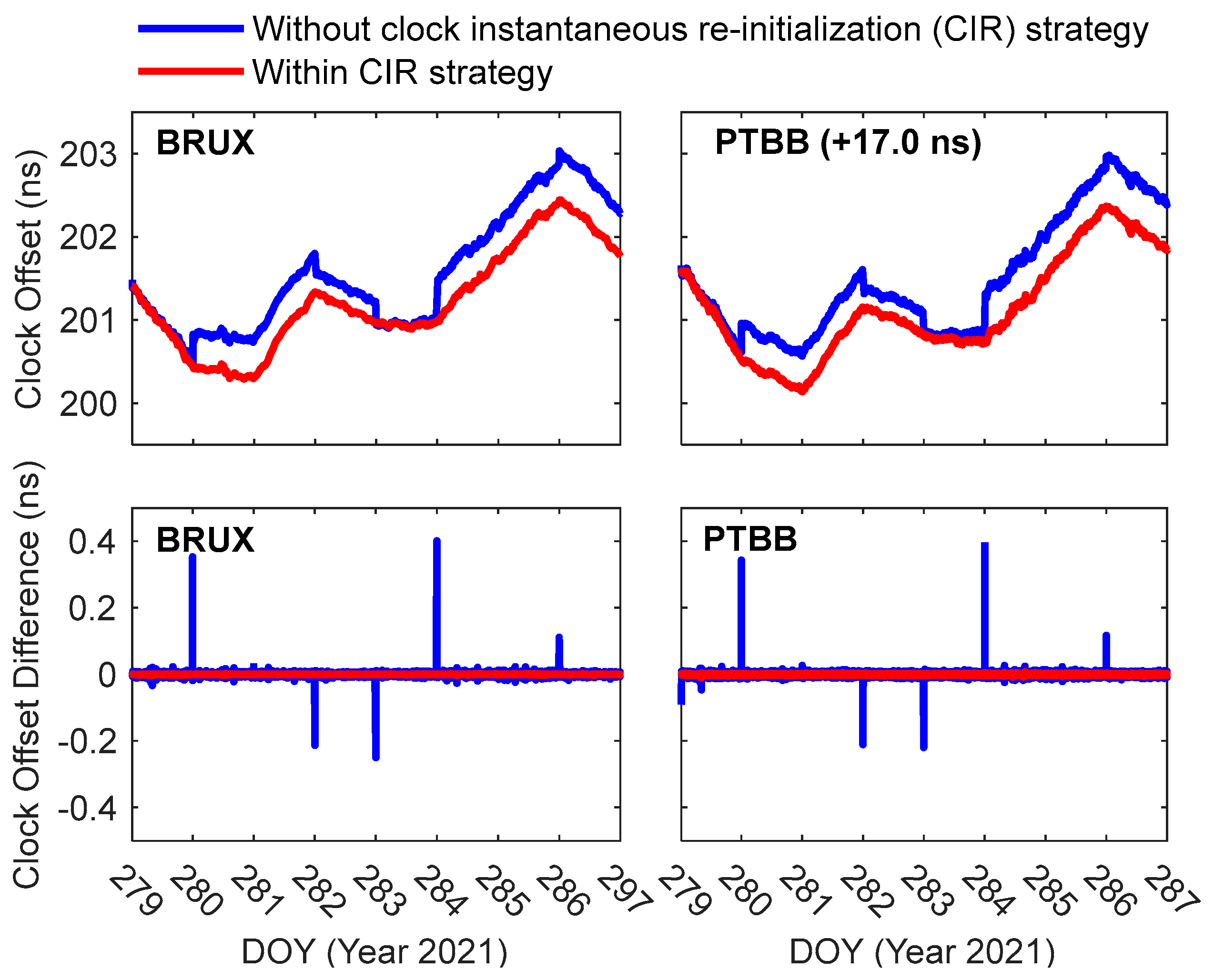
2.3. Clock Instantaneous Re-Initialization Strategy

Due to discontinuities in precise satellite products at day boundaries, receiver clock offsets estimated by traditional models tend to absorb part of these jumps. However, since observation conditions vary across stations, the amount of jump absorbed by each receiver clock differs, making it impossible to eliminate day-boundary jumps through between-station differencing fully.
Conventional studies on GNSS PPP time transfer with RCM, required initializing clock offset parameters at day boundaries and re-estimating receiver clock offsets as white noise. This approach caused part satellite clock offset jumps to be absorbed into time transfer results, leading to discontinuities at day boundaries and degrading time transfer accuracy. This study employs a Clock Instantaneous Re-initialization (CIR) strategy based on an RCM to address this issue. The strategy leverages the strong correlation between receiver clock offset and ambiguity parameters to absorb day-boundary jumps in clock offset estimations via ambiguity parameters, thereby restoring the continuity of time transfer.
Implementing the CIR strategy involves the following steps: First, reset all ambiguity parameters at the day boundary epoch (k) and assign them relatively large variances (104 m2/s2). Subsequently, reinitialize the RCM using the method researched by Stein et al. [46]. The prior clock offset dtk, the initial frequency offset dfk, and the covariance QW for initializing the RCM are as follows [46]:
d t k = d t k 1
d f k = τ 1 + τ 2 τ 1 d t k 1 d t k 2 τ 2 τ 2 τ 1 d t k 2 d t k 3 τ 1 + τ 2
Q W = q 0 τ 1 + 2 τ 2 τ 2 τ 1 + τ 2 q 0 τ 1 + 2 τ 2 τ 2 τ 1 + τ 2 q 0 2 τ 1 4 + 8 τ 1 τ 2 + 10 τ 1 2 τ 2 2 + 4 τ 1 τ 2 3 + 2 τ 2 2 τ 1 2 τ 2 2 τ 1 / τ 2 2 q 0 + τ 1 3 + 4 τ 1 2 τ 2 + 4 τ 1 τ 2 2 + τ 2 3 τ 1 τ 2 τ 1 + τ 2 q 1 + τ 2 3 q 2
where dtk−3, dtk−2, and dtk−1 are the estimated receiver clock offsets at the day boundary of the previous three consecutive epochs, where τ1 represents the time interval between dtk−3 and dtk−2, and τ2 represents the time interval between dtk−2 and dtk−1. Apart from the state parameters of the RCM and the ambiguity parameters, the initial values and prior variances of all other parameter estimates can be inherited from the epoch immediately preceding the day boundary.
The receiver clock offset parameter can achieve rapid and accurate convergence using the CIR strategy, thanks to the high-precision prior information. Meanwhile, the reset ambiguity parameters, characterized by relatively large variances, can absorb the discontinuities in satellite clock products at day boundaries. This approach ultimately realizes the objective of continuous receiver clock offset estimation.

3. Data Selection and Processing Strategies

Four stations (BRUX, PTBB, SPT0, and USN7) are selected from the IGS MGEX network to conduct the PPP time transfer experiment with the refined clock model. These stations were chosen primarily for their high-precision hydrogen atomic clocks, critical roles as key nodes in international time transfer networks, and consistently excellent observation data quality and time transfer accuracy. Specifically, BRUX, PTBB, SPT0, and USN7 are stations of the UTC time-keeping laboratories ORB (Observatoire Royal de Belgique), PTB (Physikalisch-Technische Bundesanstalt), RISE (Research Institutes of Sweden AB), and USNO (United States Naval Observatory), respectively. Taking USN7 as the centre, three time and frequency links, namely USN7-BRUX, USN7-PTBB, and USN7-SPT0, are formed to verify the time transfer performance of the refined clock model. The observation period is 8 days (DOYs 279–286 in 2021), and the observation sampling interval is 30 s. The CNES GRG precise clock and orbit products are used for data processing. The geographical distribution of these stations and the basic information are shown in Figure 1 and Table 1.
To verify the time transfer performance of the refined clock model, this research conducts experiments of PPP using the model without the refined clock model (receiver clock offset estimated as white noise), within the one-state refined clock model and the two-state refined clock model, respectively, which are denoted as RCM0, RCM1, and RCM2. By performing piecewise least squares fitting on the Allan variance of the station clock offsets provided by the IGS, the noise coefficients q0, q1, and q2 of the atomic clocks at the selected stations are calculated. The Allan deviations (ADEV) corresponding to the observation sampling interval of 30 s are obtained from the fitting coefficients, and the specific values are shown in Table 2.
GPS and Galileo raw code and carrier phase observation noises are set to 0.3 m and 3.0 mm, respectively; elevation-dependent weighting for the observations was applied. Since the IGS antenna correction product does not provide receiver-side antenna phase center offset (PCO) and phase center variation (PCV) correction parameters for Galileo, and considering the similar or identical signal frequencies between GPS and Galileo, this study herein employs GPS receiver-side antenna PCO and PCV correction parameters to approximate those for Galileo’s receiver-side antenna. The detailed processing strategies are summarized in Table 3.

4. Results

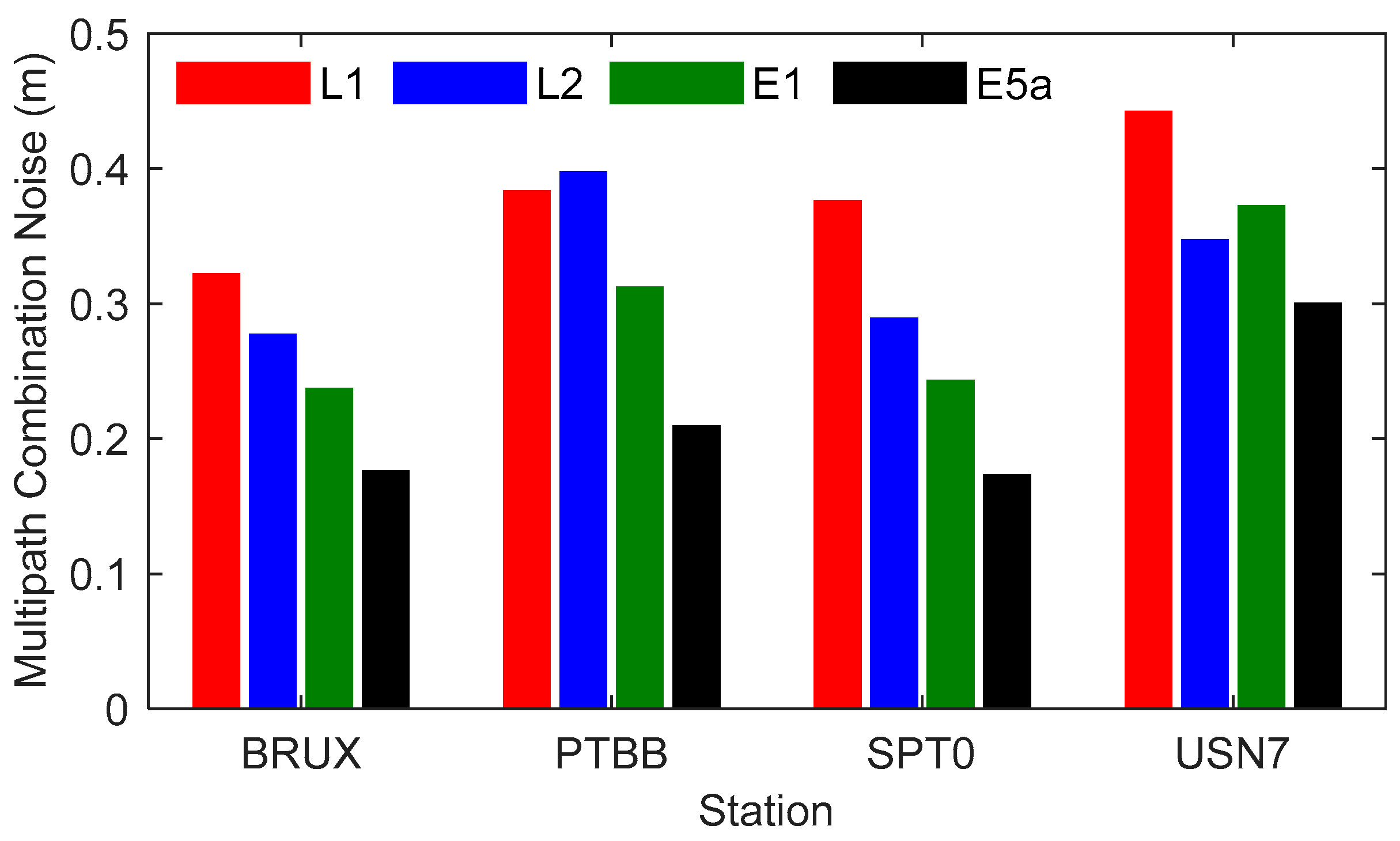
4.1. Quality Assessment of Observation

As shown in Figure 2, the number of satellites at the experimental stations is relatively similar. The number of satellites in the GPS/Galileo combination can reach about 16, and the number of GPS satellites is slightly higher than that of Galileo satellites. The average number of satellites in the GPS/Galileo combination at the stations of BRUX, PTBB, SPT0, and USN7 is 16.3, 16.2, 16.9, and 15.9, respectively, with SPT0 having marginally the highest number and USN7 slightly fewer. The Time Dilution of Precision (TDOP) values across all stations are comparable, predominantly clustered around 0.6. The mean TDOP values for the GPS/Galileo combination at BRUX, PTBB, SPT0, and USN7 stations are 0.61, 0.63, 0.61, and 0.65, respectively. USN7 exhibits a slightly higher TDOP, corresponding to its marginally lower average satellite number than the other three stations.
As shown in Figure 3, the magnitudes of the MPC (multi-path combination) noise at each station are relatively close, all within 0.5 m. The mean RMS values for GPS L1, L2, and Galileo E1 and E5a are 0.381 m, 0.327 m, 0.291 m, and 0.214 m, respectively. The MPC noise at the L1 frequency is the largest, while that at the E5a frequency is the smallest. The mean MPC noises for BRUX, PTBB, SPT0, and USN7 are 0.253 m, 0.325 m, 0.270 m, and 0.365 m, respectively. Among them, the MPC noise at BRUX is slightly smaller, and the noise at USN7 is slightly larger.

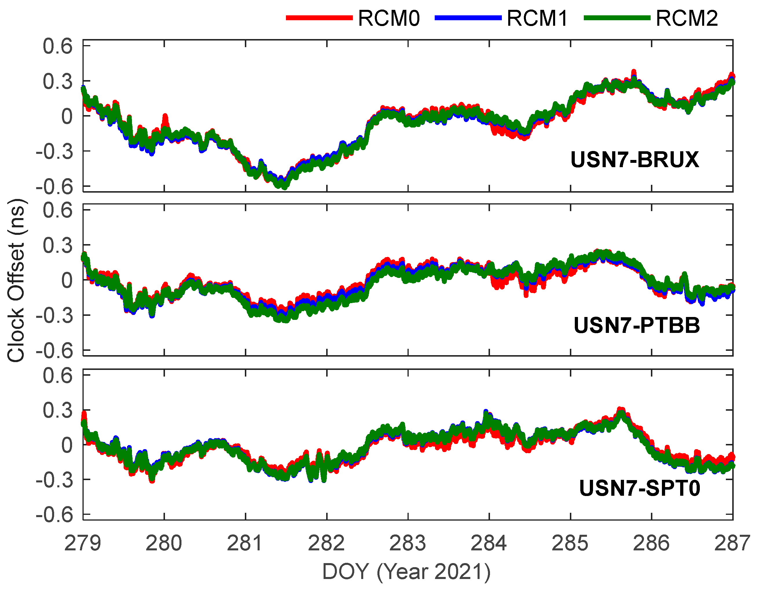
4.2. PPP Time Transfer with Refined Clock Model

Due to space limitations, Figure 4 only shows the receiver clock offset sequences of the BRUX and PTBB stations without and within the CIR strategy. It can be found that the traditional algorithm (without CIR) demonstrates a jump ranging from −0.2 ns to 0.4 ns at the daily boundary. In contrast, the CIR strategy successfully eradicates this jump at the daily boundary, rendering the clock offsets more continuous. This phenomenon validates the efficacy of the CIR strategy in eliminating the daily boundary jump. When the CIR strategy is implemented, the standard deviations (STDs) following epoch-to-epoch differencing at the BRUX and PTBB stations are 0.6 ps and 1.3 ps, respectively. Compared to the STDs of the traditional algorithm, these values are decreased by 88.6% and 77.2%, respectively, which indicates that the CIR strategy reduces the noise in time transfer and enhances the accuracy. Considering the advantage of the CIR strategy in attenuating the jump at the daily boundary, the CIR strategy will be adopted in the refined model in the subsequent experiment.
Figure 5 depicts the clock offset sequences of the three links after eliminating the corresponding trend terms from the initial clock offsets. The clock offset trends in RCM0, RCM1, and RCM2 are generally consistent. Nevertheless, the outcomes of RCM1 and RCM2 exhibit greater smoothness and stability. For instance, around DOY 284.5, there are some abrupt jumps in the data of RCM0, whereas RCM1 and RMC2 have effectively suppressed such sudden changes. Moreover, when juxtaposed with RCM0, the clock offset sequence of RCM1 demonstrates enhanced continuity. This distinctive feature gives rise to an overall divergence between RCM0 on the one hand and RCM1 and RCM2 on the other hand during specific time intervals.
Table 4 presents the STDs of the discrepancies between each scheme’s time transfer outcomes and the IGS clock offsets. Evidently, relative to RCM0, the STDs of RCM1 and RCM2 exhibit a downward trend. Specifically, the reduction rates are 7.4% for RCM1 and 10.3% for RCM2 on average. Notably, the STD of RCM2 is marginally higher than that of RCM1. This deviation may be attributed to the accuracy of the fitting coefficients for clock offset noise in RCM2. After implementing the refined clock model, significant decreases are observed in the average STD values. Specifically, the reduction rates are 5.6%, 15.1%, and 5.4%, respectively, in USN7-BRUX, USN7-PTBB, and USN7-SPT0 links.
As shown in Figure 6, the frequency stability of the time transfer after applying the refined clock model has been significantly improved, especially in terms of short term frequency stability. Taking the USN7-BRUX link as an example, the frequency stabilities of RCM0 at 30 s, 60 s, and 120 s are 2.26 × 10⁻¹³, 1.30 × 10⁻¹³, and 7.67 × 10⁻¹⁴, respectively. In contrast, the frequency stabilities of RCM1 at the corresponding moments are 4.82 × 10⁻¹⁴, 4.04 × 10⁻¹⁴, and 3.43 × 10⁻¹⁴, respectively, and those of RCM2 at the corresponding moments are 2.78 × 10⁻¹⁴, 2.44 × 10⁻¹⁴, and 2.34 × 10⁻¹⁴, respectively. Compared with RCM0, the frequency stabilities of RCM1 and RCM2 have been improved by more than half an order of magnitude in the short term. The improvement effect of RCM2 on short term frequency stability is better than that of RCM1, which may be because RCM2 adds constraints to the state transition matrix, and its constraints are stronger than those of RCM1. As time increases, the differences in frequency stability among RCM0, RCM1, and RCM2 gradually decrease, and their frequency stabilities at 120,000 s are the same.
Figure 7 illustrates the mean values of the stability gain at different moments. The average magnitudes of the stability improvement for RCM1 and RCM2 are 23.7% and 30.2%, respectively. Both RCM1 and RCM2 exhibit the most significant improvement in short term stability. For RCM1, the improvement magnitudes at 30 s, 60 s, 120 s, and 240 s are 76.2%, 66.3%, 51.3%, and 26.2%, respectively. Correspondingly, for RCM2, the magnitudes at these moments are 85.8%, 79.0%, 66.5%, and 41.6%, respectively. However, the refined clock model has a relatively minor improvement in long term stability. The improvement magnitudes of RCM1 and RCM2 at 60,000 s and 120,000 s are around 2.0%. Although the improvement magnitude of RCM2 is higher than that of RCM1 before 3000 s, the two become quite close in terms of the improvement magnitude after 12,000 s. Additionally, the improvement magnitudes of RCM2 at 60,000 s are slightly smaller than those of RCM1.

4.3. PPP Time Transfer with Refined Clock Model and Ambiguity Resolution

This study utilizes the wide-lane Satellite Bias and Integer-Recovered Clock products provided by CNES to conduct time transfer experiments using undifferenced ambiguity resolution within and without refined clock models in a GPS/Galileo combined system.
As shown in Figure 8, after adopting the refined clock model, the RMS value of the narrow-lane ambiguity residuals shows a slight downward trend compared with the unrefined scheme, with a decline of approximately 0.001 cycles. Meanwhile, the proportion of residuals distributed within the range of ±0.15 cycles has increased by about 0.1%. This result indicates that the refined clock model plays a positive role in accurately separating ambiguity parameters, significantly improving the calculation accuracy of ambiguity parameters. In addition, since the CIR strategy resets the ambiguity parameters at the daily boundary, the ambiguity parameters absorb the jumps of the satellite clock products, which may lead to the inability of the ambiguity parameters to be quickly fixed at the epoch of the daily boundary. Furthermore, this situation results in the ambiguity fixing rate when using the refined clock model being slightly lower than that of the conventional scheme.
Figure 9 and Table 5 present the comparative results between the time transfer solutions and the IGS products. Since the IGS only provided the clock offset of the PTBB station on DOY 294, Figure 9 shows the clock offsets of the USN7-PTBB link for a single day. To display the results of each scheme, Figure 9 performs a global shift on the results of the RCM1 and RCM2 schemes. The results reveal that each scheme exhibits highly consistent trends in the variations of clock offsets. Notably, the ambiguity resolution integrated with the refined clock model demonstrates enhanced robustness and reliability compared to the conventional solution. This superiority is particularly evident around DOY 284 for the USN7-BRUX link and around DOY 285 for the USN7-SPT0 link.
The statistical results show that the STD of the RCM1 and RCM2 schemes is slightly lower than that of the traditional scheme. Specifically, compared with the RCM0, the STD of RCM1 and RCM2 decreases by approximately 4.7% and 4.9% on average, respectively. Among them, in the BRUX-PTBB link, the improvement effect of RCM1 on the accuracy is the most remarkable. These findings comprehensively confirm the technical advantages of the refined clock model in the PPP ambiguity resolution time transfer. Moreover, through a comparison of Table 4 and Table 5, the accuracy of the ambiguity resolution is 22.4% higher than that of the float solution on average, which attests to the superiority of the ambiguity resolution in time transfer applications.
As shown in Figure 10, the frequency stability of the RCM1 and RCM2 has been significantly improved compared with that of the RCM0, especially the improvement effect in the short term, which is the most obvious. For instance, at the USN7-BRUX link, during the averaging time of 30 s to 300 s, the ADEV corresponding to the refined clock model scheme is distinctly lower than that of the traditional scheme. This phenomenon could be attributed to the refined clock model suppressing the observation noise, significantly boosting the short term stability. With the increase of the averaging time, the improvement range of the frequency stability of the refined clock scheme compared with the unrefined clock scheme shows a gradually decreasing trend, and the long term frequency stabilities of the two schemes are the same. Additionally, the frequency stability of RCM2 is superior to that of RCM1, which is generally consistent with the results from PPP float time transfer. This consistency can be attributed to the fact that RCM2 employs a more rigorous model than RCM1.
Table 6 shows the mean frequency stability characteristics for the three links USN7-BRUX, USN7-PTBB, and USN7-SPT0 in time transfer. It can be observed that when the averaging time is less than 3000 s, the frequency stability improves most rapidly (e.g., the ADEV of RCM0 decreases from 2.2 × 10⁻¹³ to 1.6 × 10⁻¹⁴). When the averaging time exceeds 30,000 s, the frequency stabilities of the RCM0, RCM1, and RCM2 schemes approach each other, with their variation ranges narrowing to extremely small values and gradually tending to a stable state. Statistically, compared with the RCM0 scheme, the mean frequency stabilities of RCM1 and RCM2 improved by 21.7% and 27.5%, respectively. The improvement is most significant in the short term (averaging time < 1000 s), reaching 60.7% and 70.2%, respectively; in the medium term (1000 s ≤ averaging time ≤ 10,000 s), the improvements are 13.6% and 21.7%; while in the long term (averaging time > 10,000 s), the improvements are only 2.6% and 2.7%. This result indicates that the RCM strategy mainly optimizes the frequency stability in the short term (with the maximum improvement exceeding 70%). In contrast, its effect on long term stability is relatively limited. Compared to the PPP ambiguity float time transfer solutions, the ambiguity fixed solutions of RCM1 and RCM2 show slightly inferior performance in improving frequency stability, with the stability improvement being approximately 2.5% lower than that of the PPP float solutions. This phenomenon may be related to the ambiguity fixing rate not reaching 100% and, second, to the fact that the receiver clock offsets parameters absorbing the receiver phase biases after ambiguity resolution. In addition, the refined clock model is highly sensitive to prior variance, which may lead to over-constraint problems and affect time transfer performance. Therefore, a reasonable method for determining prior variance still needs further exploration.

5. Discussion

This study establishes a time transfer model based on undifferenced GPS/Galileo combined PPP ambiguity float and fixed solutions, comparing the time transfer accuracy and frequency stability between traditional white-noise receiver clock offset estimation and refined first-order (one-state) versus second-order (two-state) clock error models. The findings reveal that refined clock models exhibit significant sensitivity to prior noise parameters covariance configuration. Suboptimal selection of excessively small prior noises may induce over-constraint issues, leading to systematic biases in time transfer. Furthermore, the refined clock model demonstrates applicability only under stable clock performance conditions. Any clock reset or adjustment necessitates a recalibration of prior noise coefficients, constraining the model’s operational versatility. Consequently, developing adaptive prior noise coefficient determination methodologies remains a critical research frontier.
Additionally, while this investigation focuses on two primary clock noise components (WFM and RWFM), comprehensive modeling incorporating other clock noise types warrants further exploration. Analysis of time transfer outcomes indicates that although the two-state model offers theoretical rigor—yielding marginally superior time transfer accuracy and frequency stability compared to the one-state model, particularly in short term stability enhancement—it introduces increased computational complexity. In multi-GNSS integration scenarios, the two-state model necessitates additional ISB parameters. Consequently, developing refined ISB parameterization strategies compatible with advanced clock models is a pivotal challenge for future research.

6. Conclusions

Leveraging the physical noise characteristics of atomic clocks, this study established an undifferenced GPS/Galileo PPP time transfer model incorporating one-state and two-state refined clock methods with the CIR method. By selecting three time transfer links composed of four MGEX stations (BRUX, PTBB, SPT0, and USN7), the performance of precise time transfer under refined clock models was evaluated using PPP ambiguity float solutions and ambiguity resolutions. Experimental results reveal that the refined clock strategies effectively mitigate receiver clock offset discontinuities at daily boundaries induced by satellite products, achieving average improvements of 6.7% in time transfer accuracy and 25.8% in frequency stability compared to conventional models. The enhancement is most significant for short term frequency stability, with stability improvements reaching 78.3%, 70.2%, 56.8%, and 33.2% at 30 s, 60 s, 120 s, and 300 s averaging times, respectively. The improvement gradually diminishes as the averaging time increases, showing less than 2% enhancement at 3000 s and 120,000 s averaging times. Additionally, the two-state refined clock model slightly outperforms the one-state model, demonstrating 11.5%, 8.0%, and 0.2% better frequency stability in short term, medium-term, and long term periods, respectively. Consequently, the two-state refined clock model is recommended for applications prioritizing high-precision time transfer and enhanced short term stability performance.
With the continuous advancement of atomic clocks towards miniaturization and cost reduction, equipping many IGS stations with high-precision hydrogen clocks is becoming increasingly feasible. Against this backdrop, the RCM based on clock characteristics is set to see broader applications in high-precision time transfer and positioning. Compared with traditional algorithms, RCM can enhance time transfer accuracy and frequency stability, thereby directly improving time-frequency signals’ synchronization and timing capabilities. This holds critical significance for 5G communication synchronization and UTC maintenance fields.
Additionally, in recent years, with the growing research interest in using GNSS time-frequency signals to determine geopotential and orthometric height, the importance of high-precision time-frequency transfer has become increasingly prominent. Theoretical research [55] indicates that the enhancement in time-frequency transfer stability brought by RCM will equivalently improve the accuracy of determining geopotential and orthometric height using time-frequency signals. The undifferenced time transfer technology incorporating RCM is expected to provide critical technical support for achieving centimeter-level cross-sea height transfer and promoting the future unification of global elevation benchmarks.

Author Contributions

Conceptualization, W.X.; methodology, C.Y.; software, W.X.; validation, W.X., C.Y., P.Z. and L.W.; formal analysis, W.X.; investigation, W.X.; resources, C.Y.; data curation, L.W.; writing—original draft preparation, W.X. and J.C.; writing—review and editing, C.Y. and L.W.; visualization, W.X., P.Z. and J.C. All authors have read and agreed to the published version of the manuscript.

Funding

This work is supported by the National Natural Science Foundation of China (No. 42304095; No. 42030105), the Key Project of Natural Science Research in Universities of Anhui Province (No. 2023AH051634), the Chuzhou University Research Initiation Fund Project (No. 2023qd07, No. 2023qd08), and the China Postdoctoral Science Foundation (No. 2024M752480).

Data Availability Statement

The GPS and Galileo observations are available at ftp://igs.gnsswhu.cn/pub/gps/data/daily/ (accessed on 1 April 2025).

Acknowledgments

We thank the IGS and CNES for providing precise satellite orbit and satellite clock offset products and GNSS observations used in this research.

Conflicts of Interest

The authors declare no conflict of interest.

References

  1. Allan, D.W.; Weiss, M.A. Accurate time and frequency transfer during common-view of a GPS satellite. In Proceedings of the 34th Annual Symposium on Frequency Control, Philadelphia, PA, USA, 28–30 May 1980; pp. 334–346. [Google Scholar]
  2. Zhang, M.; Lü, J.; Bai, Z.; Jiang, Z.; Chen, B. An overview on GNSS carrier-phase time transfer research. Sci. China-Tech. Sci. 2020, 63, 589–596. [Google Scholar] [CrossRef]
  3. Zumberge, J.F.; Heflin, M.B.; Jefferson, D.C.; Watkins, M.M.; Webb, F.H. Precise point positioning for the efficient and robust analysis of GPS data from large networks. J. Geophys. Res.-Solid Earth 1997, 102, 5005–5017. [Google Scholar] [CrossRef]
  4. Ray, J.; Senior, K. IGS/BIPM pilot project: GPS carrier phase for time/frequency transfer and timescale formation. Metrologia 2003, 40, S270. [Google Scholar] [CrossRef]
  5. Dow, J.M.; Neilan, R.E.; Rizos, C. The international GNSS service in a changing landscape of global navigation satellite systems. J. Geod. 2009, 83, 191–198. [Google Scholar] [CrossRef]
  6. Defraigne, P.; Baire, Q. Combining GPS and GLONASS for time and frequency transfer. Adv. Space Res. 2011, 47, 265–275. [Google Scholar] [CrossRef]
  7. Zhang, P.; Tu, R.; Zhang, R.; Gao, Y.; Cai, H. Combining GPS, BeiDou, and Galileo satellite systems for time and frequency transfer based on carrier phase observations. Remote Sens. 2018, 10, 324. [Google Scholar] [CrossRef]
  8. Zhang, P.; Tu, R.; Han, J.; Gao, Y.; Zhang, R.; Lu, X. Characterization of biases between BDS-3 and BDS-2, GPS, Galileo and GLONASS observations and their effect on precise time and frequency transfer. Meas. Sci. Technol. 2020, 32, 035006. [Google Scholar] [CrossRef]
  9. Tu, R.; Hong, J.; Zhang, P.; Zhang, R.; Fan, L.; Liu, J.; Lu, X. Multiple GNSS inter-system biases in precise time transfer. Meas. Sci. Technol. 2019, 30, 115003. [Google Scholar] [CrossRef]
  10. Lyu, D.; Zeng, F.; Ouyang, X. Time transfer algorithm using multi-GNSS PPP with ambiguity resolution. Chin. Astron. Astrophys. 2020, 44, 371–382. [Google Scholar]
  11. Ge, Y.; Ding, S.; Dai, P.; Qin, W.; Yang, X. Modeling and assessment of real-time precise point positioning timing with multi-GNSS observations. Meas. Sci. Technol. 2020, 31, 065016. [Google Scholar] [CrossRef]
  12. Lyu, D.; Zeng, F.; Ouyang, X.; Zhang, H. Real-time clock comparison and monitoring with multi-GNSS precise point positioning: GPS, GLONASS and Galileo. Adv. Space Res. 2020, 65, 560–571. [Google Scholar] [CrossRef]
  13. Wang, S.; Zhao, X.; Ge, Y.; Yang, X. Investigation of real-time carrier phase time transfer using current multi-constellations. Measurement 2020, 166, 108237. [Google Scholar] [CrossRef]
  14. Xu, W.; Yan, C.; Zhang, P.; Chen, J.; Qiu, D.; Liang, L.; Tao, J. Real-ime undifferenced precision time transfer of multi-GNSS and multi-frequency. Meas. Sci. Technol. 2025, 36, 025005. [Google Scholar] [CrossRef]
  15. Shi, J.; Gao, Y. A comparison of three PPP integer ambiguity resolution methods. GPS Solut. 2014, 18, 519–528. [Google Scholar] [CrossRef]
  16. Banville, S.; Geng, J.; Loyer, S.; Schaer, S.; Springer, T.; Strasser, S. On the interoperability of IGS products for precise point positioning with ambiguity resolution. J. Geod. 2020, 94, 10. [Google Scholar] [CrossRef]
  17. Mi, X.; Zhang, B.; El-Mowafy, A.; Wang, K.; Yuan, Y. Undifferenced and uncombined GNSS time and frequency transfer with integer ambiguity resolution. J. Geod. 2023, 97, 13. [Google Scholar] [CrossRef]
  18. Baudiquez, A.; Defraigne, P.; Gertsvolf, M.; Guo, J.; Jian, B.; Meynadier, F.; Tagliaferro, G. Comparison between four integer ambiguity resolved PPP GNSS time transfer software solutions. Metrologia 2025, 62, 025009. [Google Scholar] [CrossRef]
  19. Petit, G.; Kanj, A.; Loyer, S.; Delporte, J.; Mercier, F.; Perosanz, F. 1 × 10⁻¹⁶ frequency transfer by GPS PPP with integer ambiguity resolution. Metrologia 2015, 52, 301. [Google Scholar] [CrossRef]
  20. Petit, G.; Kanj, A.; Harmegnies, A.; Loyer, S.; Delporte, J.; Mercier, F.; Perosanz, F. GPS frequency transfer with IPPP. In Proceedings of the 2014 European Frequency and Time Forum (EFTF), Budapest, Hungary, 12–16 April 2014; pp. 451–454. [Google Scholar]
  21. Petit, G. Sub-10−16 accuracy GNSS frequency transfer with IPPP. GPS Solut. 2021, 25, 22. [Google Scholar] [CrossRef]
  22. Petit, G.; Defraigne, P. Calibration of GNSS stations for UTC. Metrologia 2023, 60, 025009. [Google Scholar] [CrossRef]
  23. Xu, W.; Shen, W.; Cai, C.; Li, L.; Wang, L.; Ning, A.; Shen, Z. Comparison and evaluation of carrier phase PPP and single difference time transfer with multi-GNSS ambiguity resolution. GPS Solut. 2022, 26, 58. [Google Scholar] [CrossRef]
  24. Ren, Z.; Lyu, D.; Gong, H.; Peng, J.; Huang, X.; Sun, G. Continuous time and frequency transfer using robust GPS PPP integer ambiguity resolution method. GPS Solut. 2023, 27, 82. [Google Scholar] [CrossRef]
  25. Qin, W.; Yang, H.; Zhang, Z.; Wei, P.; Yang, X. The analysis on time transfer of GPS/Galileo/BDS PPP with integer ambiguity resolution. Phys. Scr. 2024, 99, 025011. [Google Scholar] [CrossRef]
  26. Zhang, R.; Tu, R.; Ge, Y.; Wang, S.; Lu, X. An investigation into multi-frequency ambiguity resolution for real-time PPP time and frequency transfer. Meas. Sci. Technol. 2025, 36, 045003. [Google Scholar] [CrossRef]
  27. Su, K.; Jin, S. Triple-frequency carrier phase precise time and frequency transfer models for BDS-3. GPS Solut. 2019, 23, 86. [Google Scholar] [CrossRef]
  28. Zhang, P.; Tu, R.; Gao, Y.; Zhang, R.; Han, J. Performance of Galileo precise time and frequency transfer models using quad-frequency carrier phase observations. GPS Solut. 2020, 24, 40. [Google Scholar] [CrossRef]
  29. Ge, Y.; Cao, X.; Shen, F.; Yang, X.; Wang, S. BDS-3/Galileo time and frequency transfer with quad-frequency precise point positioning. Remote Sens. 2021, 13, 2704. [Google Scholar] [CrossRef]
  30. Xu, W.; Yan, C.; Chen, J. Performance evaluation of BDS-2/BDS-3 combined precise time transfer with B1I/B2I/B3I/B1C/B2a five-frequency observations. GPS Solut. 2022, 26, 80. [Google Scholar] [CrossRef]
  31. Ge, Y.; Zhou, F.; Liu, T.; Qin, W.; Wang, S.; Yang, X. Enhancing real-time precise point positioning time and frequency transfer with receiver clock modeling. GPS Solut. 2019, 23, 20. [Google Scholar] [CrossRef]
  32. Ge, Y.; Dai, P.; Qin, W.; Yang, X.; Zhou, F.; Wang, S.; Zhao, X. Performance of multi-GNSS precise point positioning time and frequency transfer with clock modeling. Remote Sens. 2019, 11, 347. [Google Scholar] [CrossRef]
  33. Ge, Y.; Wang, Q.; Wang, Y.; Lyu, D.; Cao, X.; Shen, F.; Meng, X. A new receiver clock model to enhance BDS-3 real-time PPP time transfer with the PPP-B2b service. Satell. Navig. 2023, 4, 8. [Google Scholar] [CrossRef]
  34. Lyu, D.; Zeng, F.; Ouyang, X.; Yu, H. Enhancing multi-GNSS time and frequency transfer using a refined stochastic model of a receiver clock. Meas. Sci. Technol. 2019, 30, 125016. [Google Scholar] [CrossRef]
  35. Qin, W.; Ge, Y.; Wei, P.; Yang, X. An approach to a clock offsets model for real-time PPP time and frequency transfer during data discontinuity. Appl. Sci. 2019, 9, 1405. [Google Scholar] [CrossRef]
  36. Qin, W.; Ge, Y.; Wang, W.; Yang, X. An approach for mitigating PPP day boundary with clock stochastic model. In Proceedings of the 2020 Joint Conference of the IEEE International Frequency Control Symposium and International Symposium on Applications of Ferroelectrics (IFCS-ISAF), New Orleans, LA, USA, 19–23 July 2020; pp. 1–5. [Google Scholar]
  37. Mikoś, M.; Kazmierski, K.; Hadas, T.; Sośnica, K. Stochastic modeling of the receiver clock parameter in Galileo-only and multi-GNSS PPP solutions. GPS Solut. 2024, 28, 14. [Google Scholar] [CrossRef]
  38. Han, J.; Zhang, J.; Zhong, S.; Lu, R.; Peng, B. PPP time transfer using an adaptive clock constraint model. Geo-Spatial Inf. Sci. 2024, 1–13. [Google Scholar] [CrossRef]
  39. Ai, Q.; Yuan, Y.; Xu, T.; Zhang, B. Time and frequency characterization of GLONASS and Galileo on-board clocks. Meas. Sci. Technol. 2020, 31, 065003. [Google Scholar] [CrossRef]
  40. Zucca, C.; Tavella, P. The clock model and its relationship with the Allan and related variances. IEEE Trans. Ultrason. Ferroelectr. Freq. Control. 2005, 52, 289–296. [Google Scholar] [CrossRef]
  41. Zucca, C.; Tavella, P. A mathematical model for the atomic clock error in case of jumps. Metrologia 2015, 52, 514. [Google Scholar] [CrossRef]
  42. Huang, G.; Zhang, Q. Real-time estimation of satellite clock offset using adaptively robust Kalman filter with classified adaptive factors. GPS Solut. 2012, 16, 531–539. [Google Scholar] [CrossRef]
  43. Hutsell, S.T. Relating the Hadamard variance to MCS Kalman filter clock estimation. In Proceedings of the 27th Annual Precise Time and Time Interval Systems and Applications Meeting, Bethesda, MD, USA, 29 November–1 December 1995; pp. 291–302. [Google Scholar]
  44. Yang, Y.; Yue, X.; Yuan, J.; Rizos, C. Enhancing the kinematic precise orbit determination of low earth orbiters using GPS receiver clock modelling. Adv. Space Res. 2014, 54, 1901–1912. [Google Scholar] [CrossRef]
  45. Wang, K.; Rothacher, M. Stochastic modeling of high-stability ground clocks in GPS analysis. J. Geod. 2013, 87, 427–437. [Google Scholar] [CrossRef]
  46. Stein, S.R.; Filler, R.L. Kalman filter analysis for real time applications of clocks and oscillators. In Proceedings of the 42nd Annual Frequency Control Symposium, Philadelphia, PA, USA, 1–3 June 1988; IEEE: Piscataway, NJ, USA, 1988; pp. 447–452. [Google Scholar]
  47. Wang, N.; Yuan, Y.; Li, Z.; Montenbruck, O.; Tan, B. Determination of differential code biases with multi-GNSS observations. J. Geod. 2016, 90, 209–228. [Google Scholar] [CrossRef]
  48. Petit, G.; Luzum, B. IERS Conventions (2010). In IERS Technical Note 36; Verlag des Bundesamts für Kartographie und Geodäsie: Frankfurt am Main/Berlin, Germany, 2010. [Google Scholar]
  49. Kouba, J. A Guide to Using International GNSS Service (IGS) Products IGS Central Bureau; Jet Propulsion Laboratory: Pasadena, CA, USA, 2009; p. 34.
  50. Mudrak, A.; De Simone, P.; Lisi, M. Relativistic corrections in the European GNSS Galileo. Aerotec. Missili Spaz. 2015, 94, 139–144. [Google Scholar] [CrossRef]
  51. Wu, J.-T.; Wu, S.C.; Hajj, G.A.; Bertiger, W.I.; Lichten, S.M. Effects of antenna orientation on GPS carrier phase. Astron. Astrophys. Trans. 1991, 18, 1647–1660. [Google Scholar] [CrossRef]
  52. Lyard, F.; Lefevre, F.; Letellier, T.; Francis, O. Modelling the global ocean tides: Modern insights from FES2004. Ocean Dyn. 2006, 56, 394–415. [Google Scholar] [CrossRef]
  53. Saastamoinen, J. Contributions to the theory of atmospheric refraction. Bull. Géod. 1972, 105, 279–298. [Google Scholar] [CrossRef]
  54. Böhm, J.; Niell, A.; Tregoning, P.; Schuh, H. Global mapping function (GMF): A new empirical mapping function based on numerical weather model data. Geophys. Res. Lett. 2006, 33, L03304. [Google Scholar] [CrossRef]
  55. Müller, J.; Dirkx, D.; Kopeikin, S.M.; Lion, G.; Panet, I.; Petit, G.; Visser, P.N. High performance clocks and gravity field determination. Space Sci. Rev. 2018, 214, 5. [Google Scholar] [CrossRef]
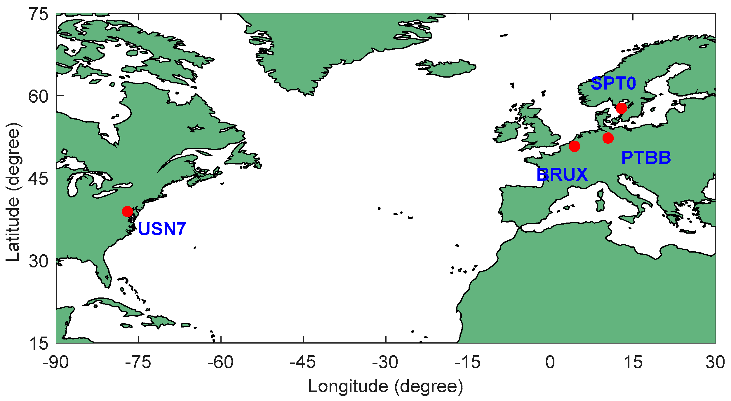
Figure 1. Geographical distribution of experimental stations.
Remotesensing 17 01910 g001
Figure 2. The number of satellites and the TDOP of the experimental station.
Remotesensing 17 01910 g002
Figure 3. The root mean square (RMS) value of multi-path combination (MPC) noise at the BRUX, PTBB, SPT0, and USN7 stations.
Remotesensing 17 01910 g003
Figure 4. The receiver clock offset sequences of BRUX and PTBB stations.
Remotesensing 17 01910 g004
Figure 5. The PPP time transfer clock offset within the refined clock model.
Remotesensing 17 01910 g005
Figure 6. Frequency stability of the PPP time transfer with the refined clock model.
Remotesensing 17 01910 g006
Figure 7. Gain of PPP time transfer stability for refined clock model.
Remotesensing 17 01910 g007
Figure 8. RMS of the narrow-lane ambiguity fractional-cycle residual and fixing rate.
Remotesensing 17 01910 g008
Figure 9. Clock offset sequences of PPP time transfer stability for refined clock model with ambiguity resolution.
Remotesensing 17 01910 g009
Figure 10. Frequency stability of PPP time transfer with the refined clock model and ambiguity resolution.
Remotesensing 17 01910 g010
Table 1. Basic information on the experimental stations.
StationReceiverAntennaCountry
BRUXSEPT POLARX5TRJAVRINGANT_DMBelgium
PTBBSEPT POLARX5TRLEIAR25.R4Germany
SPT0SEPT POLARX5TRJNSCR_C145-22-1Sweden
USN7SEPT POLARX5TRTPSCR.G5America
Table 2. Atomic clock noise coefficients and Allan deviations of the selected stations.
Stationq0q1q2ADEV
BRUX1.67 × 10−242.37 × 10−256.96 × 10−351.16 × 10⁻¹³
PTBB1.59 × 10−242.97 × 10−251.16 × 10−351.23 × 10⁻¹³
SPT01.01 × 10−231.77 × 10−259.32 × 10−352.06 × 10⁻¹³
USN79.50 × 10−236.33 × 10−251.03 × 10−332.30 × 10⁻¹³
Table 3. Details of the PPP time transfer processing strategy.
ItemStrategy
ObservationsGPS/Galileo combination; GPS: L1/L2; Galileo: E1/E5a
Elevation cutoff
Satellite orbit & clockCNES GRG final precise products
Satellite DCBCorrected by Chinese Academy of Sciences product [47]
Earth’s rotationInternational Earth Rotation Service (IERS) convention [48]
Relativistic effectCorrected: elliptical orbit and Shapiro effect [49,50]
Phase windup effectCorrected by model [51]
Tide effectCorrected [48,52]
Antenna PCO and PCVCorrected igs14.atx file
Inter-system biasEstimated as white noise (104 m2/s2)
Inter-frequency biasEstimated as constants
Station coordinateStatic, estimated as constant
Receiver clockRCM0 (estimated as white noise), RCM1 (refined one-state clock model), and RCM2 (refined two-state clock model)
Ionospheric delayFirst-order eliminated by IF combination
Tropospheric delaySaastamoinen model [53] and estimated as a random walk (10−8 m2/s2), global mapping function (GMF) [54]
AmbiguityEstimated as constant, float, and fixed solutions
Table 4. Standard deviations (STD) of the PPP time transfer with the refined clock model (ps).
LinkRCM0RCM1RCM2
USN7-BRUX32.0430.7229.80
USN7-PTBB36.2731.2130.36
USN7-SPT034.1332.9231.69
Mean34.1431.6230.62
Table 5. STDs of PPP time transfer with the refined clock model and ambiguity resolution (ps).
LinkRCM0RCM1RCM2
USN7-BRUX22.3221.5920.67
USN7-PTBB30.5228.1729.29
USN7-SPT024.4723.8723.53
Mean25.7724.5424.49
Table 6. Mean PPP time transfer frequency stability values with the refined clock model and ambiguity resolution (×10−15).
Tau/sRCM0RCM1RMC2
30229.51364.34647.524
60137.61751.78337.202
12082.09342.71631.649
30051.49538.42931.080
60039.30732.80827.977
120025.26422.06820.465
300016.21015.00314.503
60009.5548.9808.801
12,0005.6955.3705.359
30,0003.2503.1333.118
60,0003.3393.3373.323
120,0002.6972.6722.682
Disclaimer/Publisher’s Note: The statements, opinions and data contained in all publications are solely those of the individual author(s) and contributor(s) and not of MDPI and/or the editor(s). MDPI and/or the editor(s) disclaim responsibility for any injury to people or property resulting from any ideas, methods, instructions or products referred to in the content.

