Insights into Conjugate Hemispheric Ionospheric Disturbances Associated with the Beirut Port Explosion on 4 August 2020 Using Multi Low-Earth-Orbit Satellites

Abstract

In this study, we analysed remote sensing data collected during the Beirut port explosion on 4 August 2020 at 15.08 UT. For this purpose, we selected three Low-Earth-Orbit (LEO) satellite missions that passed near the Beirut port explosion site immediately after the event. The satellites involved were Swarm-B, the Defence Meteorological Satellite Program (DMSP-F17), and the Constellation Observing System for Meteorology, Ionosphere, and Climate (COSMIC-2). This study focused on identifying the possible ionospheric signatures of explosion in both hemispheres. The conjugate hemispheric points were traced using the International Geomagnetic Reference Field (IGRF) model. We found that the satellite data revealed disturbances not only over the explosion site in the Northern Hemisphere, but also in its corresponding conjugate region in the Southern Hemisphere. Ionospheric electron density disturbances were observed poleward in the conjugate hemispheres along the paths of the Swarm and DMSP satellites, whereas the magnetic field data from Swarm-B showed both equatorward and poleward disturbances. Additionally, the ionospheric disturbances detected by Swarm-B (18:52 UT) and DMSP-F17 (16:30 UT) at the same location suggested travelling ionospheric disturbance (TID) oscillations with identical spatial patterns for both satellites, whereas the disturbances observed by COSMIC-2 south of the explosion site (10°N) indicated the radial propagation of TIDs. COSMIC-2 not only recorded equatorward topside (>550 km) ionospheric electron density disturbances, but also in the conjugate hemispheres, which aligns with the time frame reported in previous studies. These ionospheric features observed by multiple LEO satellites indicate that the detected signatures originated from the event, highlighting the importance of integrating space missions for monitoring and gaining deeper insight into space hazards. The absence of equatorward ionospheric disturbances at the altitudes of DMSP-F17 and Swarm-B warrant further investigation.

1. Introduction

Coupling between the lithospheric atmosphere and ionospheric disturbances due to natural hazards, such as volcanic eruptions, earthquakes, and tsunamis, as well as artificial hazards, such as nuclear explosions, has been reported by various scientists (e.g., [1,2,3,4,5,6,7]). These studies discussed this linkage using the lithospheric–atmospheric–ionospheric coupling theory. Atmospheric gravity waves due to the explosion process and electrostatic coupling complement the full theory of ionospheric disturbances for both the created travelling ionospheric disturbances and the generated eclectic field, which propagates to the conjugate hemispheric point and likely causes mirrored ionospheric drift. Several authors have attributed the conjugate ionospheric disturbances to the E × B drift associated with earthquakes or nuclear explosions [8,9,10,11,12,13,14]. In the case of earthquake events, the electric field is thought to be generated by a complex process owing to the rupture of lithospheric rocks. Alternatively, Refs. [15,16] proposed a mechanism involving seismo-travelling atmospheric disturbances (STADs), where infrasonic waves propagate vertically into the ionosphere, altering its conductivity and thereby generating an ionospheric electric field. Ref. [17] suggested that the polarisation electric field associated with the Medium Scale Travelling Ionospheric disturbances in an airglow event is transmitted directly to its conjugate point, causing a mirrored disturbance. Despite their different perspectives on how the electric field is generated according to the phenomenon of interest, all these studies agree that it propagates along geomagnetic field lines from the epicentral region. Whether triggered by an earthquake, a nuclear explosion, or modified ionospheric conductivity, the electric field reaches its conjugate point, where it induces ionospheric drift through the E × B process [18,19,20]. Alfven wave magnetic perturbations are another mechanism of conjugate hemispheric perturbations [21]. Through this mechanism, the Alfven waves propagate along the magnetic field lines from one hemisphere, leading to plasma drift in the other hemisphere owing to electromagnetic coupling, rather than the electrostatic theory explained earlier [22]. There have been few studies on conjugate hemispheric disturbances owing to the scarcity of events and datasets. Therefore, studying such large earthquake events or nuclear explosions using different datasets and investigating their temporal and spatial behaviours would reveal more features around their ionospheric features, propagations around the epicentral point, or their propagation to its conjugate hemispheric point.

The Beirut Port, Lebanon, 2020 catastrophic chemical explosion claimed 204 lives and injured more than 7000 individuals, with a property loss of approximately 15 billion US dollars. This explosion is considered to be the largest single-fired ammonium nitrate (AN) explosion documented in history [23]. The quantities of exploded AN were estimated to be approximately 950.3 tons [24], 800–1100 tons [25], 407–936 tons [26], and 700–1000 tons [27]. This catastrophic explosion provided several indications of geosystem alteration and interactions with the ground, water, and air. Ref. [25] studied the temporal and spatial source characteristics of the Beirut 2020 explosion using seismic and acoustic methods. An extensive study based on this coupling in the case of the Beirut explosion was performed by [28]. They reported an N-shaped wave of ∼1.3 min period propagating southward at 800 m/s by confirming the ionospheric variability due to the explosion. Furthermore, Ref. [29] investigated the ionospheric disturbance caused by the blast using ionospheric total electron content observations from a Global Positioning System (GPS) satellite. They showed that the induced wave structures arrived in the ionosphere 10 ± 2 min after the explosion, which can be explained by acoustic gravity wave activity. Recently, Ref. [30] studied the atmospheric disturbances after the Beirut explosion using GNSS-derived ionospheric slant total electron content (STEC) and triaxial seismic data. Ref. [31] utilised DMSP ion density data and ionosonde data to confirm the generation of travelling ionospheric disturbances (TIDs) due to the magnetosonic waves generated from this explosion. They also demonstrated that the wave travelled more than 3000 km northwest of the explosion point.

The Beirut port explosion has attracted significant interest from several scientists because it occurred during quiet geomagnetic conditions. Therefore, investigating the dynamics of the ionosphere under the influence of this explosion is very important to the space weather community. Until now, all investigations have focused on the region within or around the explosion point; however, as far as we know, nobody has focused on whether the explosion could impact the southern hemisphere. This study seeks to provide observational evidence of conjugate disturbances associated with the Beirut port explosion that occurred on 4 August 2020. Through using multi-Low-Earth-Orbiting (LEO) satellite data during its passage close to the explosion region, such a preliminary study is invaluable for remote sensing and for inferring such distance phenomena using available instruments far from the conjugate regions of such quasi-blast explosions. The remainder of this paper is organised as follows. In Section 2, we explain the datasets and methodology. Section 3 presents the results of the study. In Section 4, we present a discussion. The final section presents the conclusions of this study.

2. Dataset and Methodology

This study used three LEO satellite missions that passed close to the explosion point (33.901°N, 35.519°E). The Swarm satellite constellation consists of three satellites, two of which (Swarm-A and Swarm-C) fly side-by-side with a separation distance of 1.4°. Its orbit is at an altitude of 420 km. The third satellite, Swarm-B, flies at a higher altitude of 520 km and has a larger inclination angle than that of the lower satellites. The three satellites have identical onboard datasets. A scalar and vector magnetometer were used to record the magnetic field, a Langmuir probe was used to record the ionospheric electron density and temperature of the particle species, and an accelerometer unit was used to record the non-gravitational accelerations [32,33,34,35]. On 4 August 2020, Swarm-B passed near the explosion at 24°E and 18:57 UT. In the current study, we used low-resolution vector magnetic field and electron density data to investigate the ionospheric variations caused by port explosions. A full description of the Level 1 swarm satellite data can be obtained from the European Space Agency website (https://earth.esa.int/eogateway/catalog/swarm-level-1-b, accessed on 1 March 2024). In addition, we used the level-2 field-aligned current (FAC) calculated from the magnetic field using Ampere’s law [36] and the level-2 ultra-low-frequency (ULF) product to confirm whether the observed disturbances at the locations and UTs of the satellite were not ULF pulsations. More information regarding ULF level-2 product data is available via the link (https://earth.esa.int/eogateway/activities/swarm-ulf-ionosphere, accessed on 1 April 2025).

The Defense Meteorological Satellite is a low-Earth polar-orbiting satellite with an altitude of 840 km and an inclination angle of 98.7°, with descending and ascending orbits of the satellite at dawn and dusk, respectively. In the current study, we used a Langmuir probe sensor onboard the satellite to investigate the ionospheric disturbance in the electron density data [31]. The ion density data were obtained from the Madrigal Database (http://cedar.openmadrigal.org, accessed on 1 December 2024) and retrieved at a 1 s cadence interval. The DMSP-F17 satellite flowed from the Southern to the Northern Hemisphere in an ascending phase within longitudes of 45°E–25°E and 15:57 UT.

COSMIC-2/FORMOSAT-7, a subsequent mission to COSMIC-1, was launched on 25 June 2019, following the success of its predecessor. The system comprises six satellites in low-Earth orbit and may provide several radio occultation (RO) soundings daily in low- and mid-latitude regions. The COSMIC-2 satellite first orbited at an altitude of approximately 720 km. It was then adjusted to a lower altitude of 550 km, while maintaining an inclination angle of 24 degrees [37]. All the six COSMIC satellites provided identical datasets. A Tri-Global Navigation Satellite System Radio Occultation Receiver was utilised to remotely detect and analyse the temperature, pressure, moisture, and lightning formation in the atmosphere from a space-based perspective. Radio occultation is a method employed to measure the electron density. The COSMIC satellites measure the deflection of radio signals transmitted by a GPS as they pass through the atmosphere. Only the COSMIC-2 paths from 15:00 UT to 16:00 UT, which are close to the longitudinal regions of the Beirut port explosion in both hemispheres, were investigated. Three profiles were investigated at approximately 15:30 UT in the Northern Hemisphere, the dip equator, and the Southern Hemisphere. The ionospheric parameters from radio occultation measurements can be distorted by solar activity, geomagnetic fluctuations, ionospheric irregularities, and atmospheric gradients below an altitude of 200 km. These effects may cause anomalies in the electron density profiles, such as missing F2-layer peaks, negative values, or severe structural disturbances. To ensure reliable analysis, it is essential to rigorously assess and exclude poor-quality profiles before using radio occultation data [38,39]. In this study, we employed the cubic spline function approach. Based on this method, we eliminated the distorted electron density profiles while retaining only the well-shaped ones, with a correlation coefficient exceeding 99%. All profiles used in the current study showed correlation coefficient >0.99 for adjacent spline sampling points from 2 to 30.

To investigate the ionospheric disturbances from satellite data, we implemented two different methods: one by calculating the first-time derivative of the observed data directly, and the other by using the cubic spline fit to remove the long wavelengths and trends from the observed raw data. The first derivative was implemented by [40,41] to highlight the disturbances caused by earthquakes, and the second and third derivatives were implemented by [14] to highlight the nuclear explosion signature in the FAC. It is worth noting that we selected 9 August 2020 and 10 August 2020, which are the quietest two days of this month, to represent the background quiet days for comparison, in addition to the hour preceding the event. The Swarm-B and COSMIC profiles of these days, according to the criteria set earlier, are shown in Figures S1–S3 in the Supplementary Materials. All profiles demonstrated minimal perturbations compared with the event day.

The cubic spline fit was recommended by [42] to subtract the long-wavelength background from the observed to obtain the residual perturbations which represent the difference between the observed data and the fit. The longest wavelength of the cubic spline fit was twice the distance between adjacent spline sampling points. In this method, a cubic spline function ($s$) smooths the observed data by minimising the following potential function:

$$p\sum w_i{|y_i-s(x_i\left)\right|}^2+\left(1-p\right)\int {\left({\displaystyle \frac{d^{2}s}{{dx}^2}}\right)}^{2}dx$$

(1)

where $p$ is the smoothing parameter, $w_i$ is the weighting factor, and $y_i$ represents the data of interest. In the current analysis, we implemented the MATLAB (version 2024b) spap2 function, which assumes equal weight and minimizes the $\sum w_i{|y_i-s(x_i\left)\right|}^2$ term. We fitted the cubic spline function twice: first to 10 data points to capture high transient variations and then to 60 data points to remove long wavelengths when feeding the residual data into the spectrum analysis. The residual, defined as the difference between the observed data and the corresponding cubic spline fit, was the target of interest. To reveal transient variations in the data, the first-time derivative was utilised as an auxiliary tool alongside the 10-data-point fitting technique.

The frequency domain of the data was analysed using the wavelet transformation technique. The wavelet transform decomposes a time-series signal into its corresponding time–frequency representation using a selected base wavelet function. The wavelet coefficients were obtained by convolving the signal with the complex conjugate of the base wavelet, as expressed in Equation (2):

$$W_n\left(s\right)=\sqrt{{\displaystyle \frac{dt}{s}}}\sum _{n=1}^N{x}_n{\psi }_n^{*}\left[\left(n-n_0\right){\displaystyle \frac{dt}{s}}\right]$$

(2)

where $dt$, s, n, and ${\psi }_n^{*}$ are the sampling time interval, scales, the shifting parameter, and the complex conjugate of the base wavelet filter, respectively. As a bandpass filter, the wavelet transform effectively isolates specific frequency components over time. Various wavelet filters exist, each with a distinct shape and frequency width. In this study, the Morlet wavelet was used owing to its balanced frequency localisation and uniform distribution. We used MATLAB’s built-in functions to examine the signal spectrum and employed the wavelet tool provided by [43] for further analysis.

To trace the geomagnetic field line between both hemispheres and identify the conjugate points, we used the International Geomagnetic Reference Field (IGRF) model. In this study, the latitudes at the beginning and end of the traced magnetic field lines were referred to as conjugate points. The magnetic field line was mapped from a point near Beirut port along the meridian path of the satellite to its conjugate point in the Southern Hemisphere, or vice versa. The IGRF toolbox is a MATLAB software (version 2024b) package available on the MathWorks website that uses the 12th generation IGRF coefficient or on the GitHub link (https://github.com/wb-bgs/m_IGRF, accessed on 21 May 2025) that uses the 14th generation IGRF coefficients.

3. Results

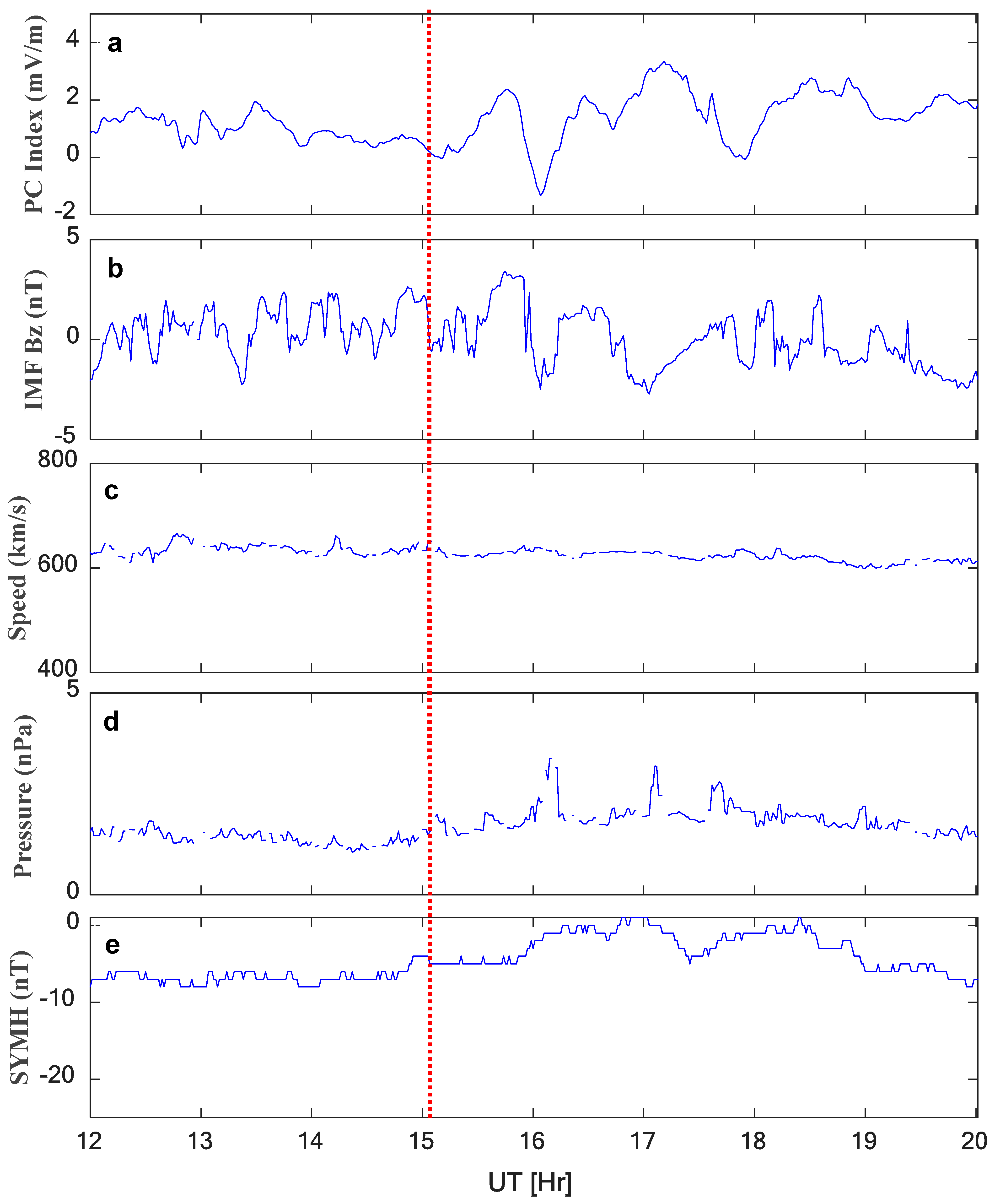
Figure 1 shows the solar wind parameters and geomagnetic activity indices for 4 August 2020. Several studies have analysed the solar wind conditions associated with the Beirut port explosion, all of which confirmed the presence of quiet conditions during the event [25]. The vertical dashed red line indicates the Beirut explosion at 15:08 UT. In this study, we further confirmed these conditions by including the Polar Cap Index, which may serve as a convenient proxy of the solar wind energy inflow into the magnetosphere and farther down to the ionosphere/atmosphere. The absolute value of the polar cap north index (PCN) during the Beirut port explosion was less than 1 (mV/m); therefore, the probability of magnetospheric energy loading was low according to a comprehensive analysis of the PC limits [44,45,46,47]. Also, the real time auroral electrojet demonstrated a low AE value (https://wdc.kugi.kyoto-u.ac.jp/ae_realtime/202008/index_20200804.html, accessed on 11 May 2025). Therefore, the probability of ionospheric disturbance from auroral regions at the time of the Beirut port explosion is extremely low. Solar wind parameters: the interplanetary magnetic field (IMF-Bz) did not decrease less than −2 nT and no sudden increase in the solar wind speed or density occurred before or during the explosion time. The symmetric (SYM-H) index, which is a high-resolution proxy for the Dst index, was close to zero. It is worth noting that the Dst index represents variations in the Earth’s magnetic field due to the magnetospheric ring current; therefore, the magnetosphere is very quiet. Generally, the quiet-time Dst index is defined to be within $\pm 20\mathrm{n}\mathrm{T}$ [36,44,48]. Subsequently, any variation in the magnetic field or ionospheric dynamics in the explosion region reflects the impact of the explosion.

3.1. Swarm Satellite Electron Density Data

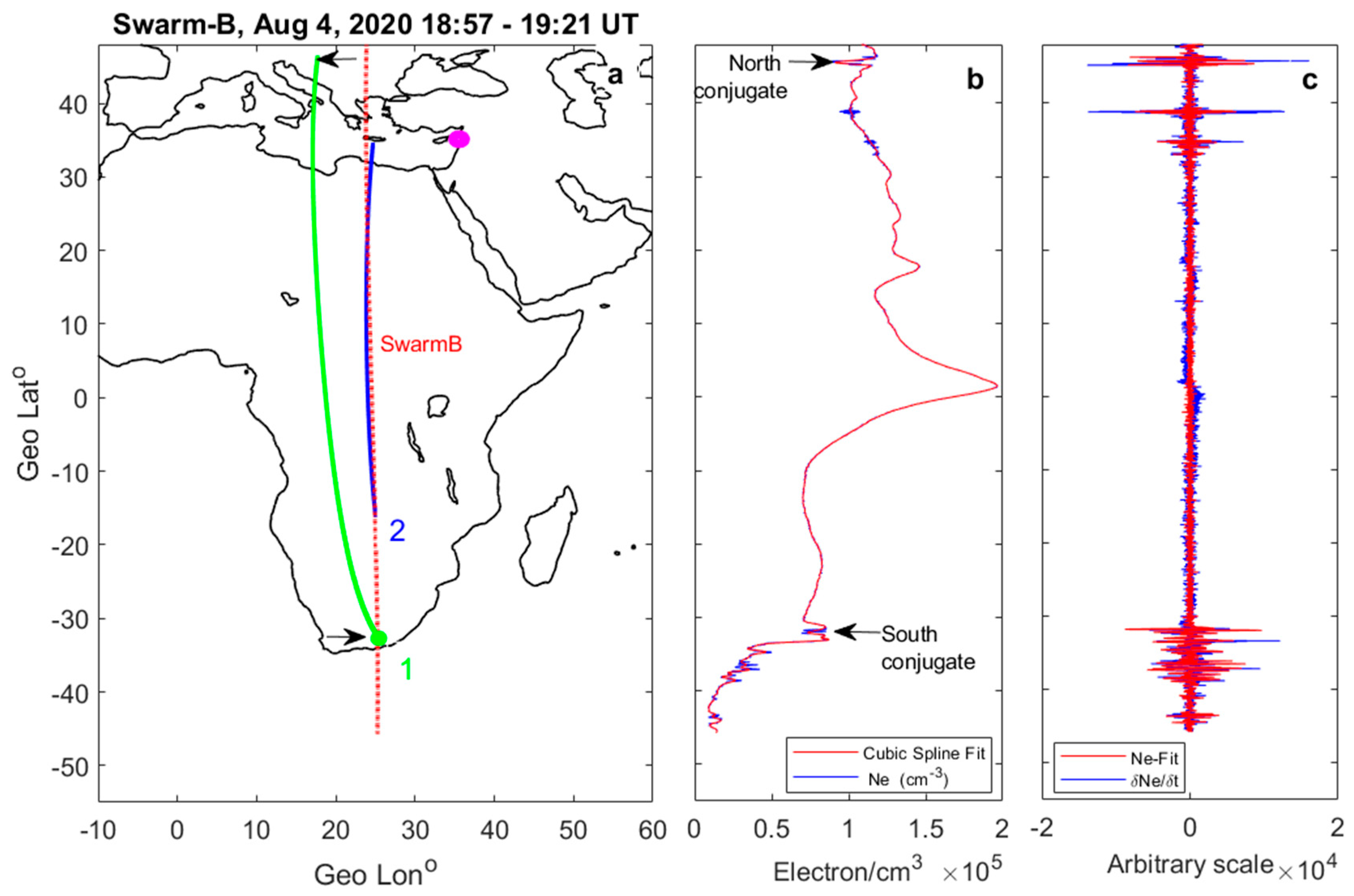
On 4 August 2020, Swarm-B passed near the explosion site at approximately 18:57 UT, heading toward the North Pole. The satellite trajectory is represented by a red line projected onto a geographical map, as shown in Figure 2. Swarm-B required approximately 30 min to traverse its path, starting from the initial point in the Southern Hemisphere at 18:57 UT and reaching the final point in the Northern Hemisphere at 19:21 UT. Specifically, the trajectory of the satellite was projected along the 24.5° magnetic meridian located 8° west of the explosion site. The explosion site is indicated with a dotted magenta symbol on the map. The traced magnetic field lines (green and blue lines) connecting the conjugated hemispheric points in the two different regions are shown in green and blue, with the initial tracing points in the Southern Hemisphere marked as 1 and 2, respectively. The endpoints of these field lines at 300 km altitude represent the conjugate hemispheric points. The green and blue traced magnetic field lines represent the conjugate perturbations in the observed electron density and magnetic field data recorded by Swarm-B along its trajectory, respectively. The black horizontal arrows indicate the latitudinal endpoints of the traced magnetic field line (green).

The ionospheric electron density observed along the path of the Swarm-B satellite, as shown in Figure 2b, demonstrates disturbances in the ionospheric density in the Northern Hemisphere, extending across a wide latitudinal range (30–60°N). In contrast, ionospheric density disturbances were also observed along the satellite’s path in the Southern Hemisphere, but were more localised, spanning a narrower latitude range (30–40°S) than that in the Northern Hemisphere. At the geomagnetic equator, the two equatorial ionospheric crests (north and south) appear asymmetric, but remain undisturbed. The first-time derivatives and residual electron densities presented in Figure 2c illustrate the exact latitudinal locations of the hemispheric perturbations. Specifically, the electron density was subtracted from a cubic spline function fitted to a 10 s interval. The 10 s interval was chosen through experimentation with the data to achieve a good location of transient variation. As a result, the residual data shown in Figure 2c represent spatial disturbances occurring at scales smaller than approximately 74 km (calculated as 10 × 7.4 km/s), where 7.4 km/s is the average velocity of the Swarm-B satellite. The first two quiet days, according to the GFZ Helmholtz Centre for Geosciences (https://kp.gfz.de/en/data; accessed on April 2024), representing the quietest days of the event month (9 and 10 August 2020) within the 15:00–19:30 UT period, were also investigated. Figure S4 in the Supplementary Materials shows that both paths exhibited clear Ne disturbances in both the Northern Hemisphere near Beirut Port and at its conjugate point in the Southern Hemisphere. These two quiet days were selected to characterise the background conditions surrounding the explosion site and its conjugate region.

3.2. Swarm Satellite Magnetic Field Data

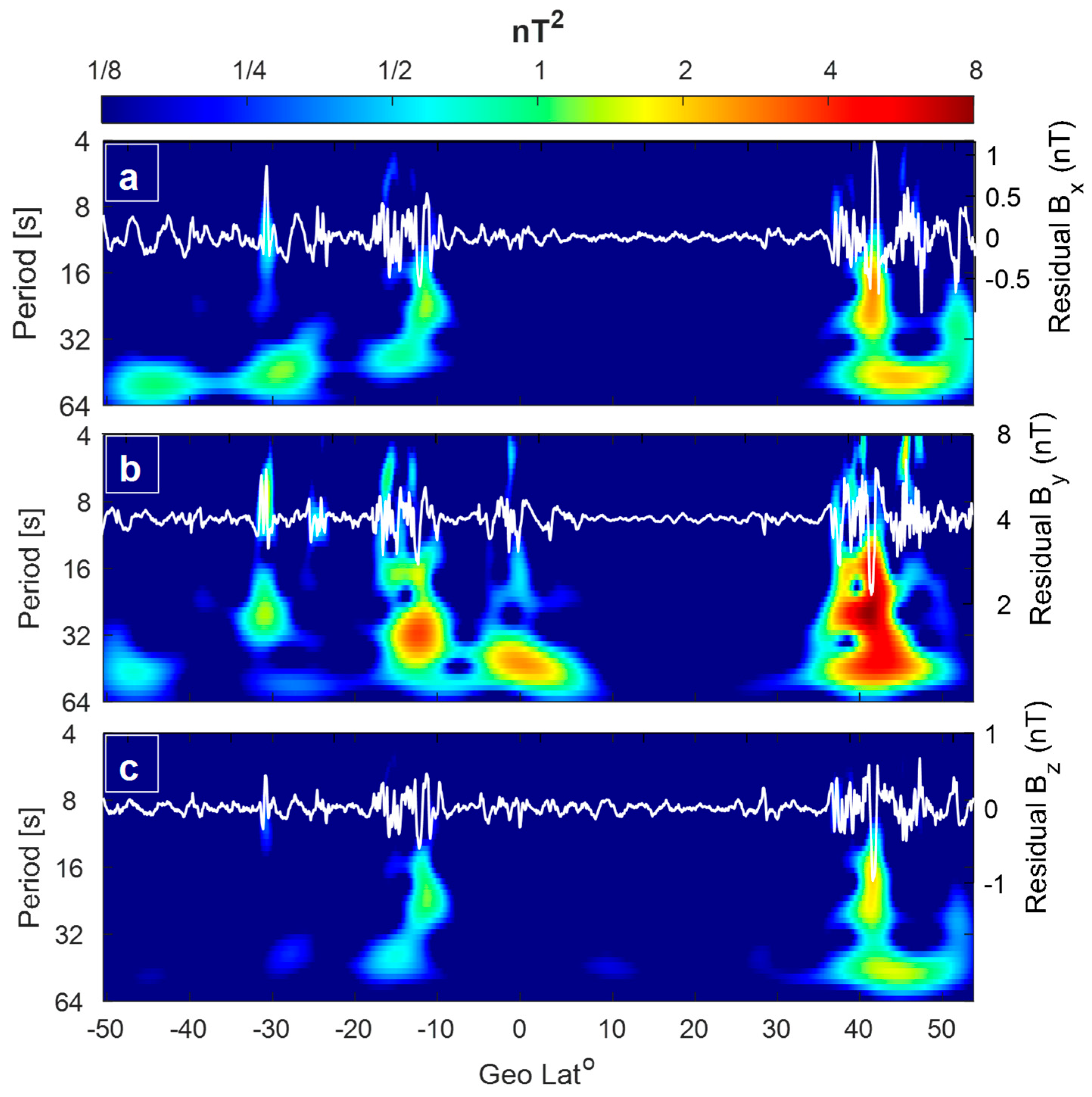
Figure 2c demonstrates that both the first-time derivative and the residual (the difference between the observed data and the fitted curve) effectively capture ionospheric disturbances. The cubic spline fitting, applied at 60 s intervals, corresponds to approximately 4° latitude along the Swarm satellite’s path. Therefore, spatial variations exceeding this scale were removed from the residuals. In addition to the ionospheric density data, magnetic field data analysis was performed. The wavelet transformation applied to the residual magnetic field data further highlights these disturbances. Figure 3a–c illustrates the residual magnetic field components as white lines superimposed on the wavelet transformation. Power intensity is represented by the coloured bar shown above the data panels. The right and left y-axes represent the amplitude in nanoteslas and the periodic time of oscillations in seconds, respectively. The maximum power spectrum of these oscillations, ranging from 30 s to 60 s, corresponded to the applied fitting interval. Wavelet transformation serves as an auxiliary tool to highlight the locations of significant magnetic perturbations in both hemispheres.

It is worth noting that we investigated ULF pulsations of the Pc3 (20–45 s) and Pc4 (45–150 s) types during this event using two different datasets. Specifically, we analysed the ULF Level-2 data product from the Swarm-B satellite, as well as ground-based magnetic data recorded by a station near Beirut port and its conjugate point, as shown in Figures S4 and S5 in the Supplementary Materials. This step was necessary to confirm that the ionospheric disturbances observed by Swarm B and the other satellites discussed in the following sections were not related to ULF pulsations. Data from both the Swarm-B ULF product and ground-based observatories PEG and HBK clearly demonstrate that the universal times (UTs) of the detected pulsations are well separated from the ionospheric disturbances recorded by the satellites.

3.3. Swarm Satellite Field Aligned Current Data

It is important to note that the FAC data are Level 2 data, derived from the magnetic field measurements of the Swarm satellite using Ampère’s law. The FAC data were archived on the Swarm Data Access Server, managed by the European Space Agency (ESA) (https://swarm-diss.eo.esa.int/, accessed on 1 December 2024). FAC strength is attributed to the difference in conductivity between the ionospheric hemispheres [33]. The steady flow of the FAC is highly sensitive to small changes in the ionospheric state, and any variations in the magnetic field are reflected in the FAC data. 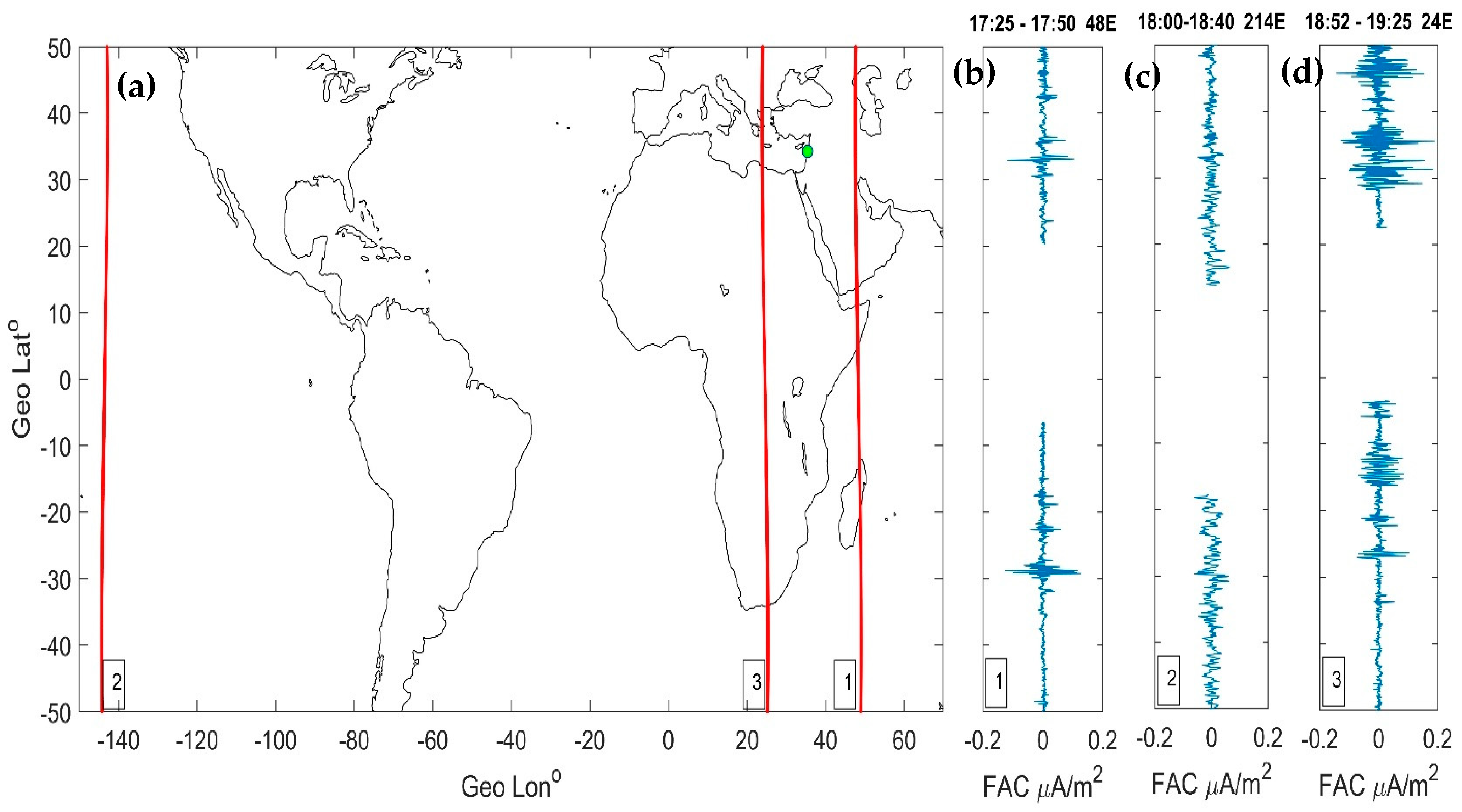Figure 4a shows the projection of Swarm-B tracks as red lines over the geographic map, and the corresponding FAC data along these three paths are displayed in the three rightmost panels (Figure 4b–d). The order of Swarm-B tracks 1, 2, and 3 is indicated in boxes adjacent to each path at the bottom of the geographic map. The FAC data showed perturbations along the first and third tracks, whereas the second track exhibited no significant disturbances. The most prominent perturbation occurred along the third track over the African continent, appearing later than the second track over the Pacific Ocean. Notably, the first and third tracks pass closer to the Beirut port explosion site, as marked by a green circle. FAC disturbances were observed not only in the northern hemisphere near the explosion site, but also at the conjugate point in the Southern Hemisphere, as indicated by the blue traced field line in Figure 4a.

The FAC data retrieved from Swarm-B along the three different paths and their corresponding wavelet transformations are shown in the upper and lower rows of Figure 5. However, the FAC data for paths 1 and 3 exhibited transient oscillations in the frequency range of 4–8 s, and the Northern and Southern hemispheric frequencies were not well-mirrored. In contrast, the FAC data for the second track exhibited significantly different behaviours, showing oscillations with a much longer periodic time range of approximately 64 s, as indicated by its high-power amplitude. This longer periodicity suggests a more stable, non-transient variation in the FAC along path 2.

3.4. DMSP-F17 Ion Density Data

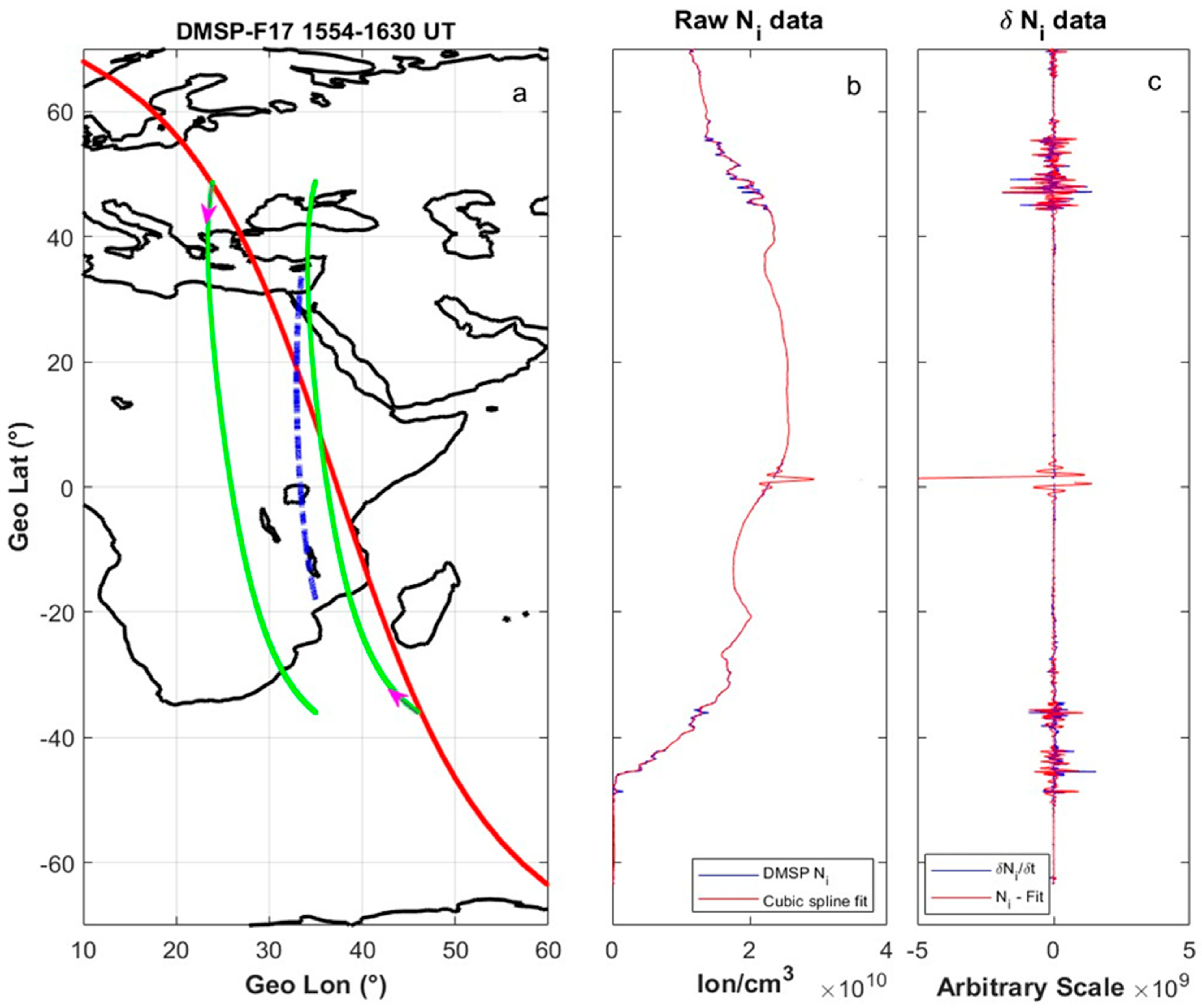
On 4 August 2024, the DMSP F17 satellite passed near the Beirut port explosion site, travelling from the Southern to the Northern Hemisphere along the longitudes 30–45°E between 15:54 UT and 16:30 UT, approximately 46 min after the explosion at 15:08 UT. The satellite trajectory is represented by the solid red line on the geographic map in Figure 6a. The middle panel shows the ion density data along the path of the satellite, with the electron density shown in blue and the cubic spline fit in red. The right panel presents the first-time derivative and residuals, where the derivative is in blue and the residual is in red. The green lines in Figure 6a represent the traced IGRF magnetic field lines connecting the Northern and Southern Hemispheres. Owing to the high inclination angle (98.7°) of the DMSP orbit, the satellite covered a wide range of longitudes. Consequently, two IGRF magnetic field lines were traced to map the disturbance regions along the DMSP-F17 path to their corresponding conjugate regions, and the last line mapped the Beirut port site to the southern hemisphere. The two green lines trace the Southern Hemisphere disturbance point along the satellite’s trajectory to its corresponding conjugate location in the Northern Hemisphere, while the other green line traces the Northern Hemisphere disturbance to its conjugate location in the Southern Hemisphere.

Arrows along the traced magnetic field lines are included to clarify the point along the path of the satellite at which the traced magnetic field line begins and mark the disturbances along the satellite paths. The traced field lines clearly connect the latitudes where the ionospheric density disturbances were observed in both hemispheres. Notably, the northern conjugate point was positioned north (40–50°N) of the Beirut Port explosion site (33.901°N).

3.5. COSMIC Satellite RO-Electron Density Data

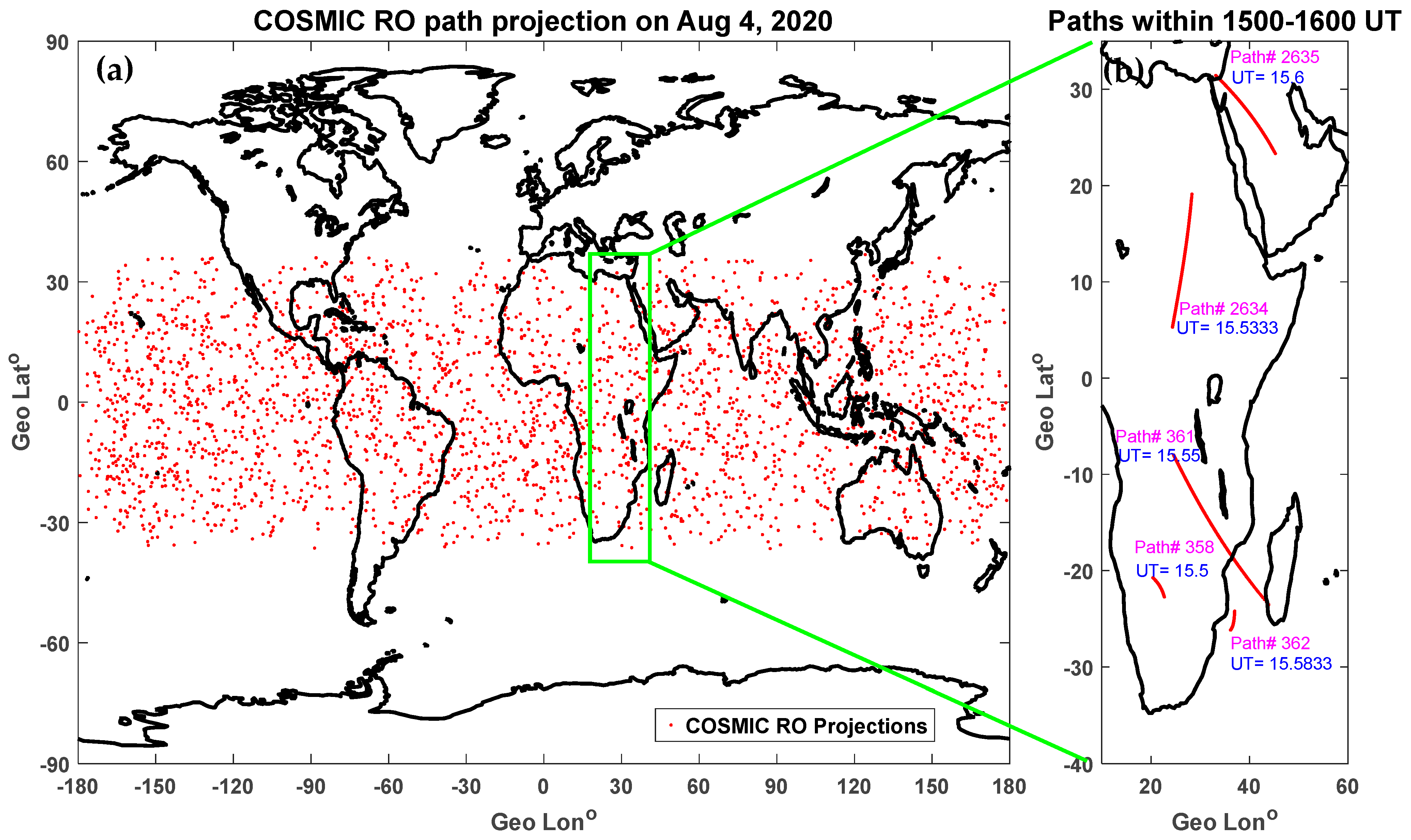
On 4 August 2024, the four COSMIC satellites generated 3000 RO profiles worldwide. The initial points of each trajectory are marked with red dots on the global map shown in Figure 7a. To examine conjugate ionospheric disturbances related to the event, only full trajectories within 10–60°E longitude, ±40° latitude, and the 15:00–16:00 UT time window were selected, as highlighted by the green box. Figure 7b shows that only five trajectories were selected based on the criteria mentioned earlier. The trajectories were projected onto the world map as red lines, with their universal time marked at the start of each path. All the selected paths were recorded at approximately 15:30 UT (15.5 h), approximately 22 min after the Beirut explosion (15:08 UT). For clarity in the analysis and comparison, the paths were numbered arbitrarily based on their archived order. The most significant trajectories in this study were 2635, 2634, and 362.

• Trajectories 2635 and 362 are expected to be located at conjugate hemispheric points;
• Trajectory 2634 lies near the dip equator and was deliberately selected to determine whether the observed perturbation was due to the mapped field line or transient variations from the travelling ionospheric disturbances.

Fortunately, this configuration of the COSMIC satellite constellation provides a valuable opportunity to capture the prompt response of conjugate hemispheric regions to the explosion.

Figure 7. (a) A geographic map of the initial location of each COSMIC path retrieved on 4 August 2020, marked in red dots. (b) The paths of COSMIC satellites within 1500–1600 UT. The path number and the universal time of each path are marked next to the start of each trajectory path.

Figure 7. (a) A geographic map of the initial location of each COSMIC path retrieved on 4 August 2020, marked in red dots. (b) The paths of COSMIC satellites within 1500–1600 UT. The path number and the universal time of each path are marked next to the start of each trajectory path.

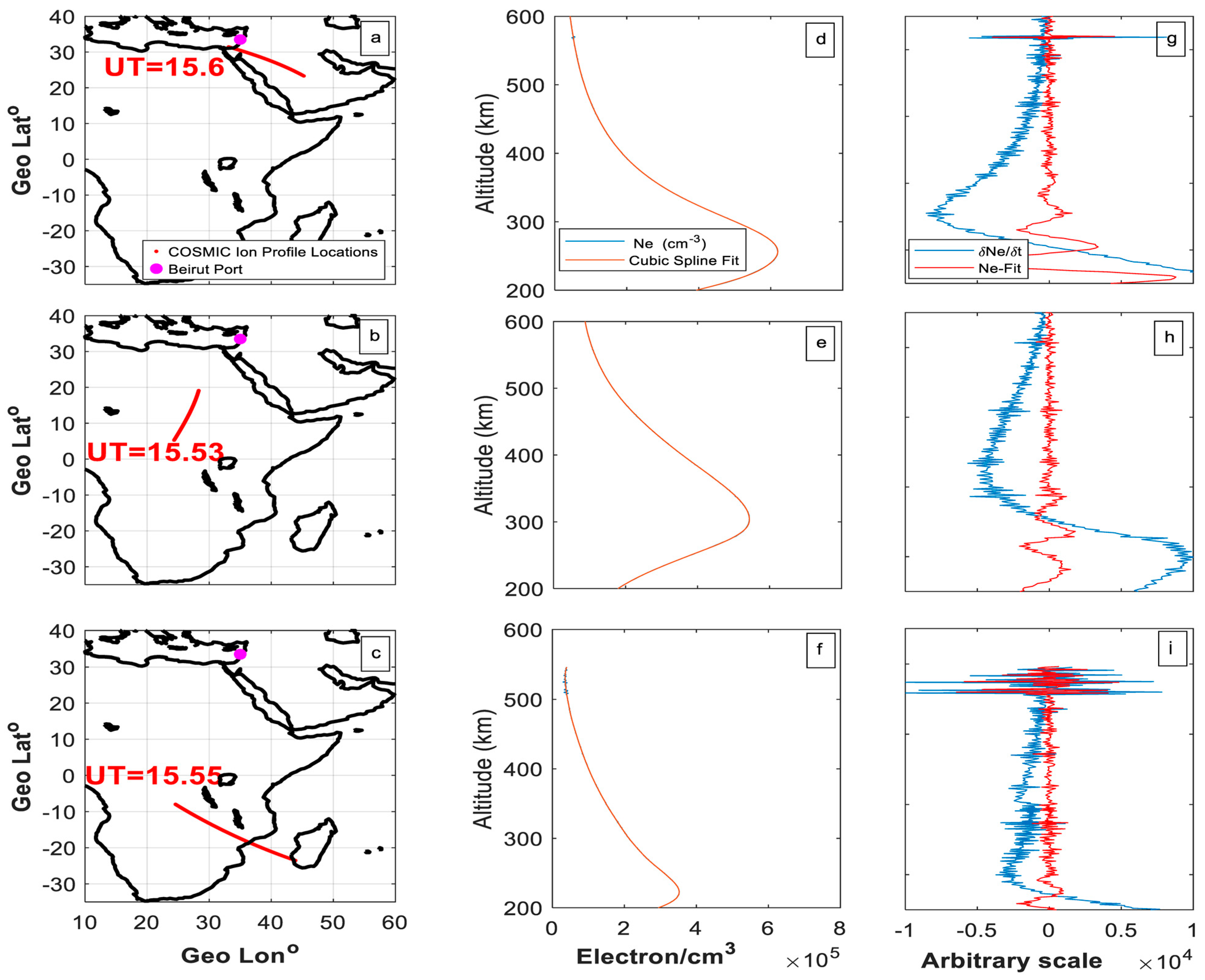
Similar to Swarm-B and DMSP-F17, the ionospheric disturbances were identified using the first-time derivative of the RO data and by subtracting the cubic spline fit from the original RO data to obtain the residual. Figure 8 presents an analysis of the three trajectories:

• 2635 at UT = 15.6 h (top row);
• 2634 at UT = 15.53 h (middle row);
• 362 at UT = 15.55 h (bottom row).

Figure 8. Trajectories of the COSMIC RO path numbers: (a) 2635, (b) 2634, and (c) 362. Dot in magenta colour indicates the position of Beirut port. The middle column (d–f) shows the corresponding electron density data (blue) with the cubic spline fit (red). The far-right column (g–i) presents variations in the COSMIC electron density data, where the red lines represent the residuals, and the blue lines indicate the first-time derivative.

Figure 8. Trajectories of the COSMIC RO path numbers: (a) 2635, (b) 2634, and (c) 362. Dot in magenta colour indicates the position of Beirut port. The middle column (d–f) shows the corresponding electron density data (blue) with the cubic spline fit (red). The far-right column (g–i) presents variations in the COSMIC electron density data, where the red lines represent the residuals, and the blue lines indicate the first-time derivative.

The left column (Figure 8a–c) displays the geographic locations of the trajectories. The middle column (Figure 8d–f) shows the RO electron density (blue) with a cubic spline fit (red). The right column (Figure 8g–i) presents the first-time derivative (blue) and residual (red). Both the residual and first-time derivative reveal clear signatures of ionospheric disturbances at higher altitudes in trajectories 2635 and 362 (top and bottom rows, respectively). However, trajectory 2634, located over the dip equator, showed no disturbances, despite its close timing to trajectory 2635. The presence of electron density perturbations in trajectories 2635 and 362 motivated us to trace the magnetic field lines between them. It is also worth noting that we investigated the COSMIC-RO profiles near Beirut Port and its conjugate location during the quietest days (9 and 10 August 2020) between 15:00 and 16:00 UT, as well as during the hour preceding the event, as shown in Figures S1 and S2 of the Supplementary Materials. All profiles from quiet days and hours preceding the event exhibited minimal perturbation.

Figure 9 illustrates the mapping of the IGRF magnetic field lines connecting the Northern and Southern Hemispheres. The red lines represent the COSMIC RO trajectories, with their corresponding universal times labelled in red. The blue lines indicate the traced magnetic-field lines. One field line connects the Beirut port explosion site (marked by the magenta dot) to the southern COSMIC trajectory, whereas the other lines link the northern COSMIC trajectory to its conjugate point in the southern hemisphere. This mapping highlights the geomagnetic connection between the ionospheric disturbances observed in both hemispheres by the COSMIC satellites.

4. Discussion

The findings presented in this study provide critical insights into the impact of characterising the ionospheric disturbances caused by the Beirut port explosion using multi-satellite observations. We analysed electron and ionospheric density data from three LEO satellites, Swarm-B, COSMIC-2, and DMSP-F17, that passed near the Beirut port explosion. The magnetic field and FAC data were examined using only Swarm-B. The IGRF-traced magnetic field lines clearly show that the ionospheric density disturbances were well-mapped between both hemispheres, as illustrated along the Swarm-B and DMSP-F17 paths in Figure 2 and Figure 6, respectively. The endpoints of these traced magnetic field lines, corresponding to the observed electron density perturbations along the satellite trajectories, were located poleward of the Beirut port site (33.5°N). No ionospheric density disturbances were detected at the altitudes of the DMSP and Swarm satellites at latitudes lower than those of the Beirut port. However, unlike Swarm and DMSP, the COSMIC-2 RO profiles at UT = 15.5 h detected electron density perturbations at altitudes of 550 km, with two COSMIC trajectories positioned equatorward of the explosion site.

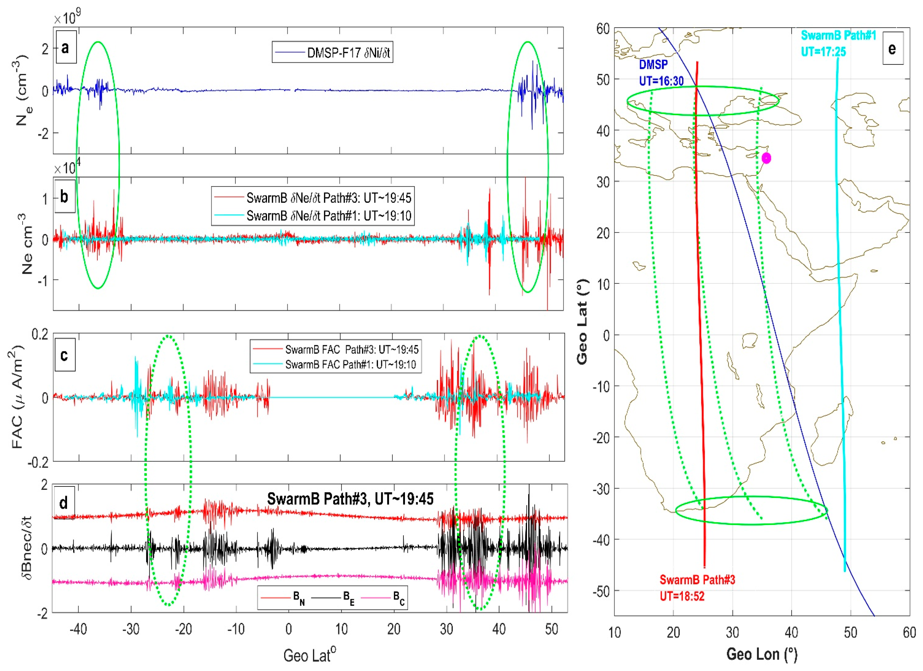
The red and cyan solid lines in Figure 10b refer to the trajectories of the Swarm-B satellite and the blue solids refer to the DMSP satellites. The dashed green lines refer to the traced magnetic field lines between the ionospheric perturbation regions in both hemispheres. The universal time for each satellite trajectory is marked in the same colour. Notably, DMSP-F17 (UT = 16:30), in conjunction with ground-based IGS observatories, confirmed the detection of TIDs at 3000 km from Beirut [31]. Similarly, this study reports these ionospheric disturbances in conjunction with Swarm-B at the same location. However, Swarm-B passed more than two hours after the DMSP, and both satellites confirmed conjugate hemispheric ionospheric disturbances, indicating the persistence and large-scale nature of these perturbations.

Unlike previous studies [28,29,31,49], this study tracked this event for an extended period after the explosion. Ionospheric disturbances caused by the explosion, detected by DMSP-F17 1.5 h after the event over the mid-latitudes, were also observed by Swarm-B at the same location, but 3.75 h after the explosion. These late coincidence observations indicated long-lasting TIDs caused by the explosion. The absence of prolonged ringing signals in the hmF2 or foF2 data, as reported in [31], may be attributed to the use of low-time-resolution data (8 min).

Overall, our results indicate that the ionospheric disturbances observed in this study exhibit clear hemispheric conjugacy, reinforcing previous assertions that such disturbances are often mirrored in both hemispheres due to interhemispheric coupling processes [14,17,29,49]. It is worth noting that [31] discussed the reason for the absence of TIDs along the path of the DMSP south of Beirut in terms of low ion neutral collision at the high altitude (850 km) of the DMSP. The absence of equatorward ionospheric Ne disturbances at the low altitude of Swarm-B (520 km) provides additional insight into the altitude range in which Ne disturbances are absent along the satellite, as shown in Figure 10b. Regardless, the space-based data showed no southward ionospheric disturbances, and ground-based studies [25,29] have reported southward disturbances related to the explosion event around UT = 15.4 h. Therefore, the lack of equatorward Ne ionospheric disturbances at the altitudes of Swarm-B and DMSP-F17 warrants further investigation using different datasets. The analysis of the FAC and magnetic field data from Swarm-B revealed distinct equatorward disturbances along path #3 (Figure 10c,d), observed both south of Beirut and in the conjugate Southern Hemisphere (elliptical green dashed lines). Despite the large amplitudes in both conjugate regions, as indicated by the dashed ellipses in Figure 10c,d, we could not confirm that these oscillations were directly related to the explosion. The passage of the satellite at dusk (19:45 LT) coincided with a significant hemispheric potential difference, naturally enhancing the FAC [33].

However, the local time conditions limited our ability to confirm whether the equatorward FAC and magnetic field ionospheric disturbances were related to the Beirut port explosion. Incorporating additional observational techniques would be valuable to provide further evidence or support any previously raised assumptions. The COSMIC technique investigates the altitudinal profile of ionospheric electron density, whereas the Swarm and DMSP techniques record in situ observations [34,50,51]. Southward, equatorial, and conjugate ionospheric disturbances observed by COSMIC were recorded at higher altitudes (>500 km) at different intervals from the explosion time. The IGRF confirmed that the disturbance observed in the Southern Hemisphere was mapped magnetically to its conjugate disturbed region in the Northern Hemisphere, as shown in Figure 9. 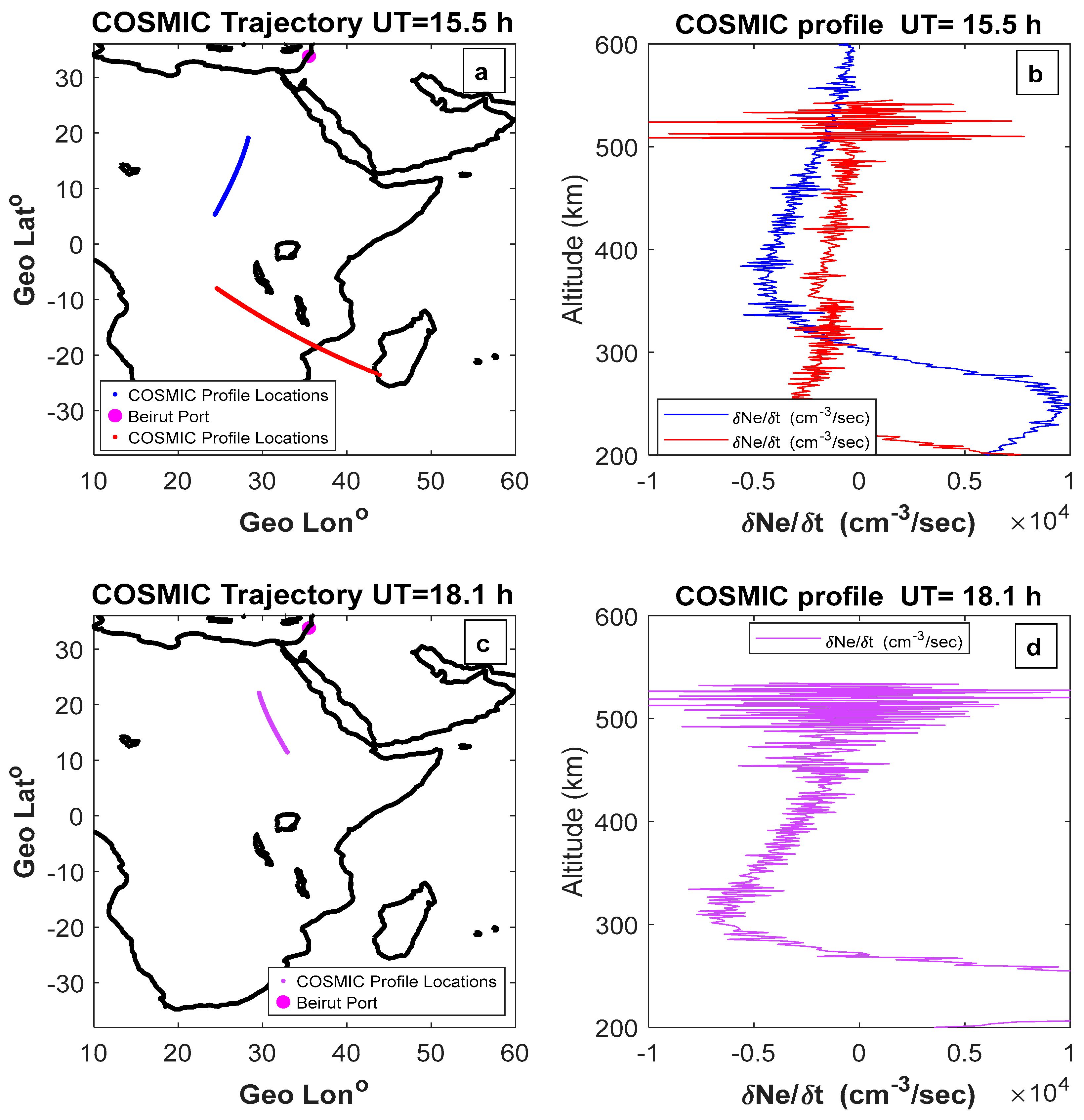Figure 11 presents the COSMIC profile locations and the rate of electron density change ($d{N}_e/dt$), illustrating significant ionospheric fluctuations at altitudes > 500 km. The red lines in Figure 11a,b represent the trajectory and variations in the ionospheric electron density at UT = 15.5 h, which were observed at the conjugate point in the Southern Hemisphere. However, the COSMIC trajectory over the equator at the same time did not simultaneously detect the ionospheric disturbances. The lower panels show the trajectory of the COSMIC satellite at UT = 18.1 h, when ionospheric disturbances were later observed over the magnetic equator (10°N). The observational patterns over the magnetic equator, where nothing was observed in DMSP and Swarm, but some signatures were captured by COSMIC RO, were generally consistent with the TID scenario presented by [31]. The low collisionality at the ionospheric topside altitude caused the TID wavefront to be highly field-aligned, and the horizontal magnetic field at the magnetic equator oriented the TID wavefronts almost horizontally flat. DMSP and Swarm (sampling the ionospheric density at a constant altitude along their respective orbits) did not detect these fluctuations. In contrast, the COSMIC RO measurements were able to capture these fluctuations because the altitude of the tangent point shifted over time during each RO event (i.e., there was an effective altitudinal scan).

Additionally, COSMIC observations detected ionospheric disturbances south of Beirut extending up to 10° latitude in the conjugate hemispheric regions. These conjugate ionospheric Ne disturbances at (30°N, 20°S) around UT ~15.5 h suggest the role of ionospheric electric fields generated at the northern hemisphere (at 30°N), which are instantaneously mapped along magnetic field lines to the southern hemisphere (20°S), subsequently initiating disturbances through the E × B process [8,17]. It is worth noting that Ref. [17] suggested that the polarisation electric field for the observed airglow event propagates normal to the medium-scale TIDs and is instantaneously transmitted to its conjugate point, leading to ionospheric drift. These disturbances are mirrored in both hemispheres. Accordingly, we ensured that these disturbances were in the conjugate hemispheric region using the previously performed IGRF mapping technique. Subsequently, we investigated the frequency-domain features of these disturbances in both the hemispheres. 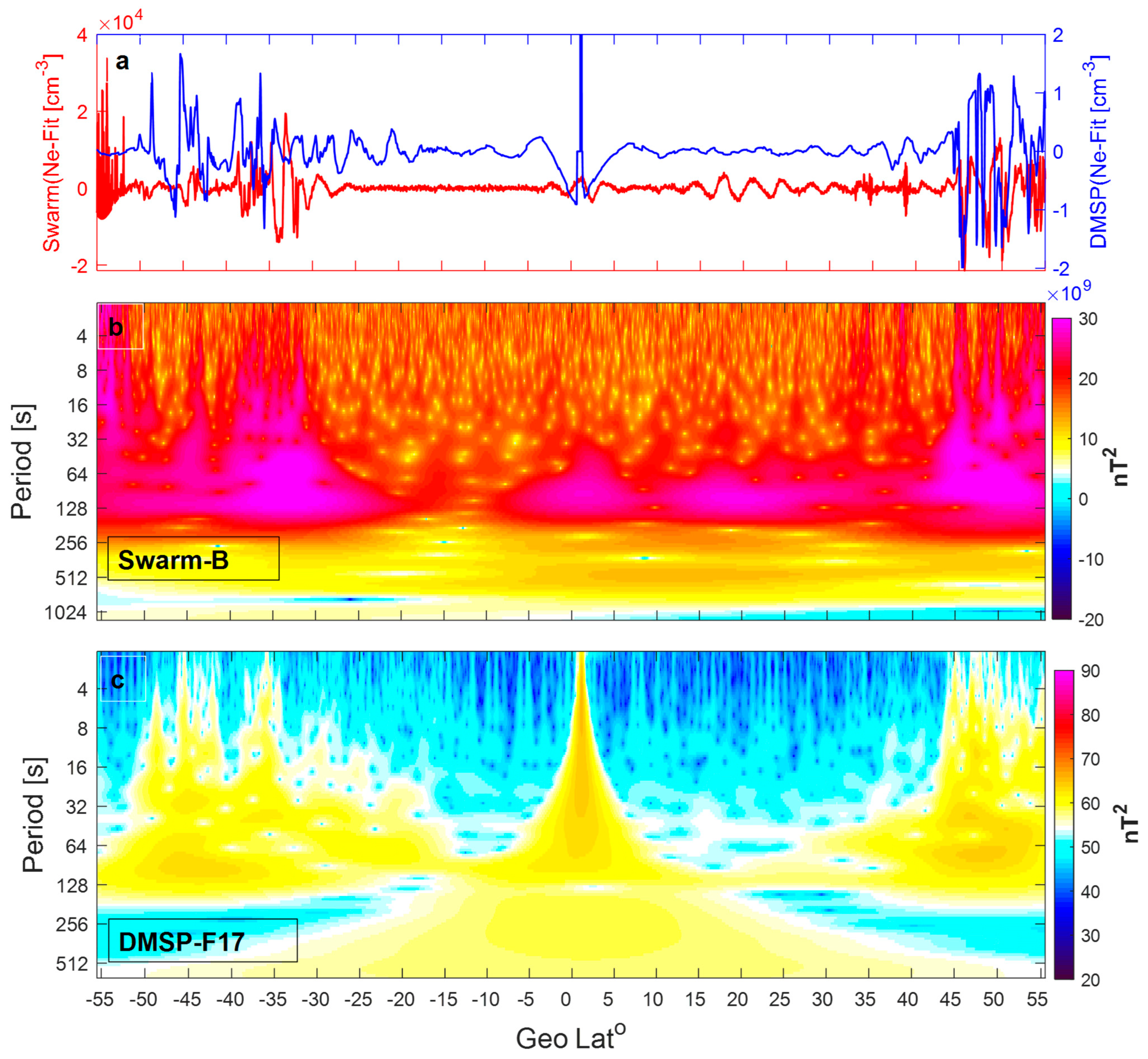The wavelet transformation of the electron density shown in Figure 12 clearly demonstrates that both the Swarm and DMSP Ne data exhibit similar periodic oscillations. These oscillations, observed by both satellites and in both hemispheres, have horizontal wavelengths of the dominant period in the range of 64–128 s. The observed similarities suggest that the electric field generated in the Northern Hemisphere propagates along magnetic field lines to the Southern Hemisphere, inducing electron density perturbations with oscillatory features that mirror those observed in the Northern Hemisphere.

In contrast, the later disturbances (UT = 18.1 h) at 10°N suggest that the propagated TIDs continued travelling southward over large radial distances from the explosion site. The observation of disturbances at higher altitudes, as detected by COSMIC, further supports the interpretations of [29], who attributed the sustained ionospheric disturbances at the altitudes of the DMSP to the lower ionospheric density, which maintained large TIDs amplitude over long distances. Further investigations and analyses are crucial for confirming whether the generation of ionospheric disturbances at equatorward sites after the explosion is related to TIDs or other mechanisms.

5. Conclusions

This study identified the conjugate ionospheric disturbances linked to the 2020 Beirut port explosion (4 August 2020, at 15:08 UT) using multisatellite data. Analysis of the ionospheric electron density, magnetic field, and FAC data from (Swarm-B, DMSP, and COSMIC-2) satellites near the explosion site and its conjugate points revealed significant findings, highlighting the value of coordinated satellite missions in space weather research.

Electron density perturbations were observed along the trajectories of DMSP (16:30 UT) and Swarm-B (18:57 UT) at locations far poleward from the explosion site in the Northern Hemisphere and at its conjugate regions in the Southern Hemisphere. The traced magnetic field lines confirm that the latitudes of these perturbations in both hemispheres are magnetically connected. Moreover, the wavelet spectrum revealed that the electron densities in the conjugate regions shared the same features in the frequency domain. However, Swarm and DMSP-F17 passed near the explosion site approximately 3 h and 1.5 h later, respectively; the prolonged and sequential observation of both satellites suggests the inertia of the ionosphere. In addition, COSMIC-2 (15:33 UT) detected electron density perturbations in the topside ionosphere (>550 km altitude) at two conjugate points (30°N and 22°S). Three hours after the explosion (18:6 UT), COSMIC also detected ionospheric electron disturbances closer to the magnetic equator, suggesting the role of the TID travelling radially.

Swarm-B’s magnetic field and FAC data showed perturbations near the explosion, extending both equatorward and poleward, as well as in the conjugate Southern Hemisphere. However, attributing these variations solely to the explosion is inconclusive, as Swarm-B’s dusk-time passage coincides with the natural FAC dynamics influenced by ionospheric conductivity gradients and large-scale hemispheric potential differences. These factors complicate the direct association between FAC perturbations and the explosion.

This study provides strong evidence for conjugate hemispheric perturbations linked to the Beirut port explosion. These perturbations were identified through multiple observational datasets and traced in both hemispheres using a magnetic field line modelled using the IGRF model. However, the absence of equatorward conjugate perturbations in the electron density at the altitudes of the Swarm and DMSP trajectories warrants further investigation in future studies. Therefore, further analysis is recommended to investigate whether the equatorward ionospheric disturbances after the explosion are related to the TIDs or other mechanisms and to investigate whether the conjugate ionospheric disturbances are related to the electrostatic polarisation ionospheric electric field perpendicular to the TID wavefront or to the electromagnetic coupling process.