


Ionospheric TEC and ROT Analysis with Signal Combinations of QZSS Satellites in the Korean Peninsula
 , , , , , and
Abstract
1. Introduction
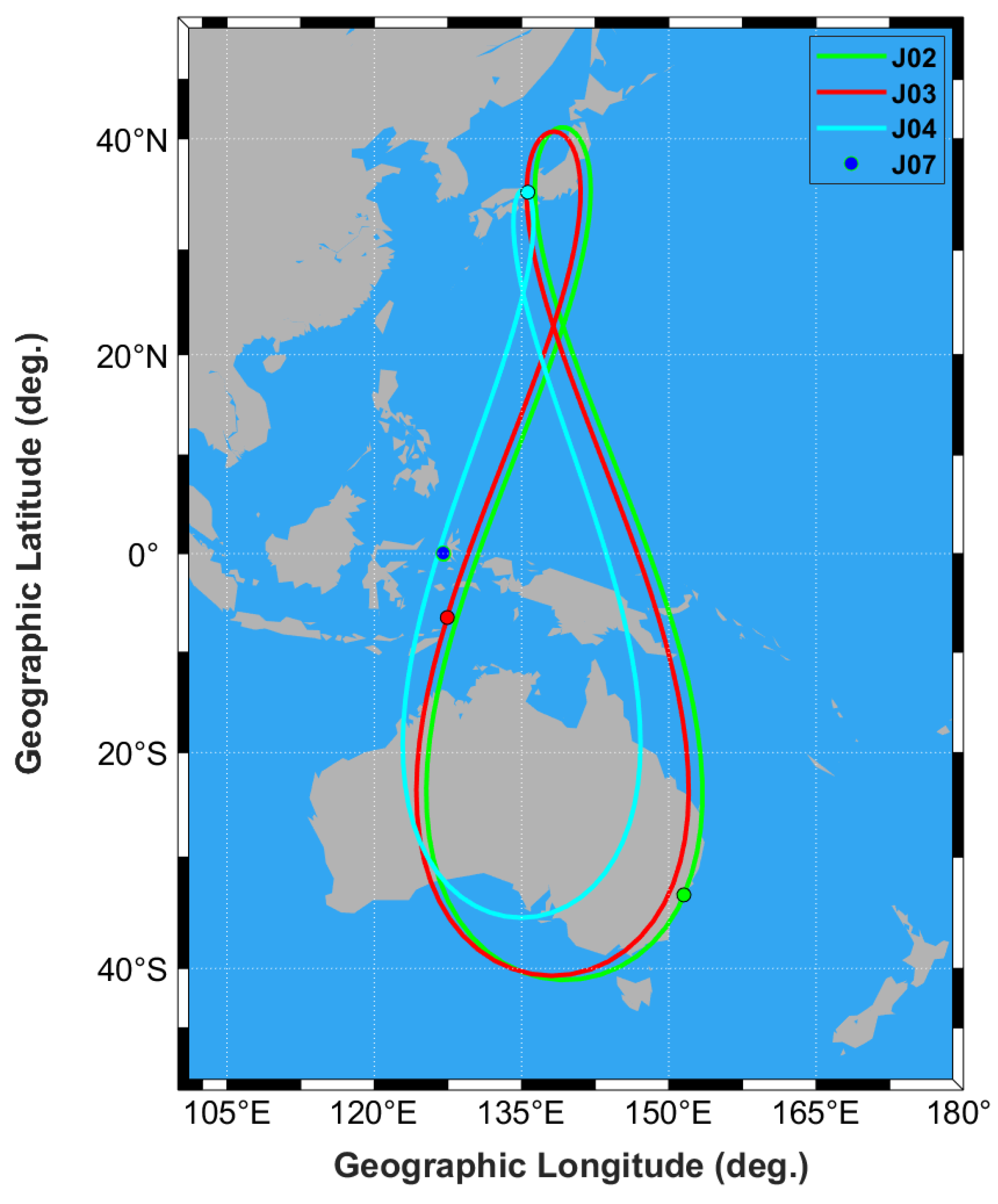
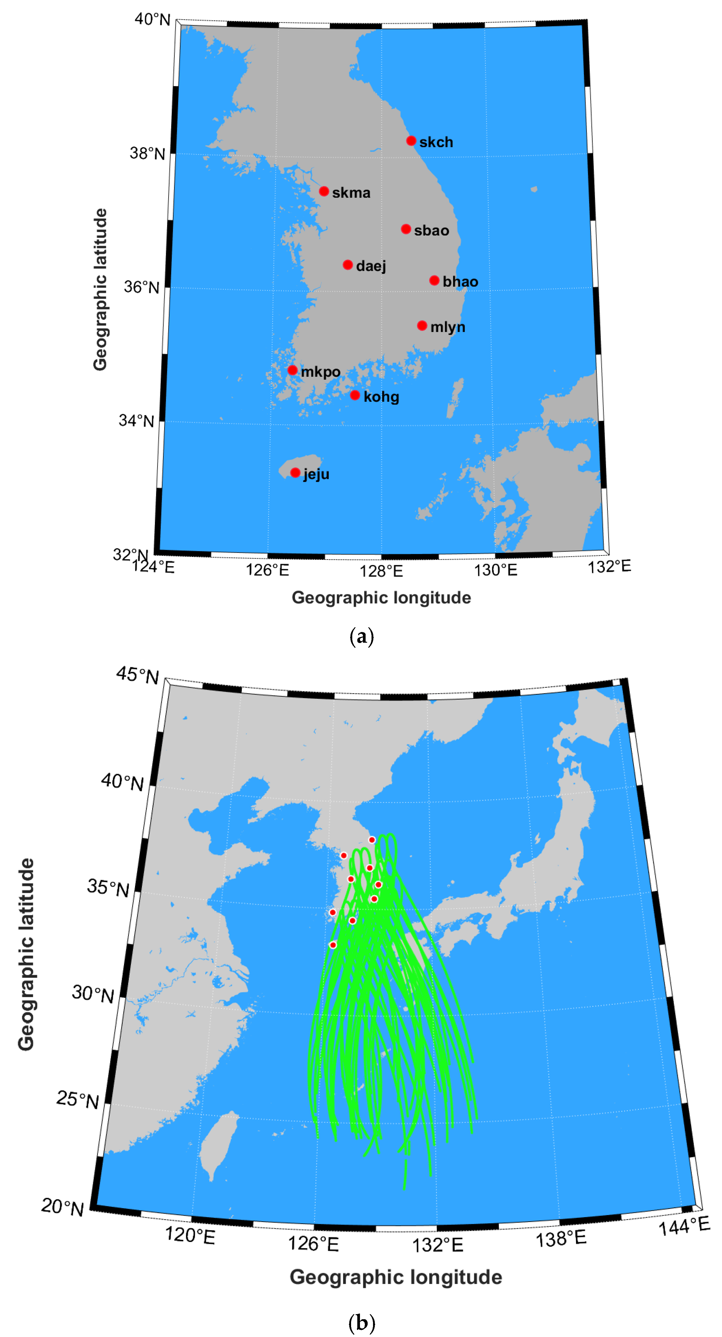
2. QZSS Constellation and Data Description
3. TEC Estimation Method
4. Results
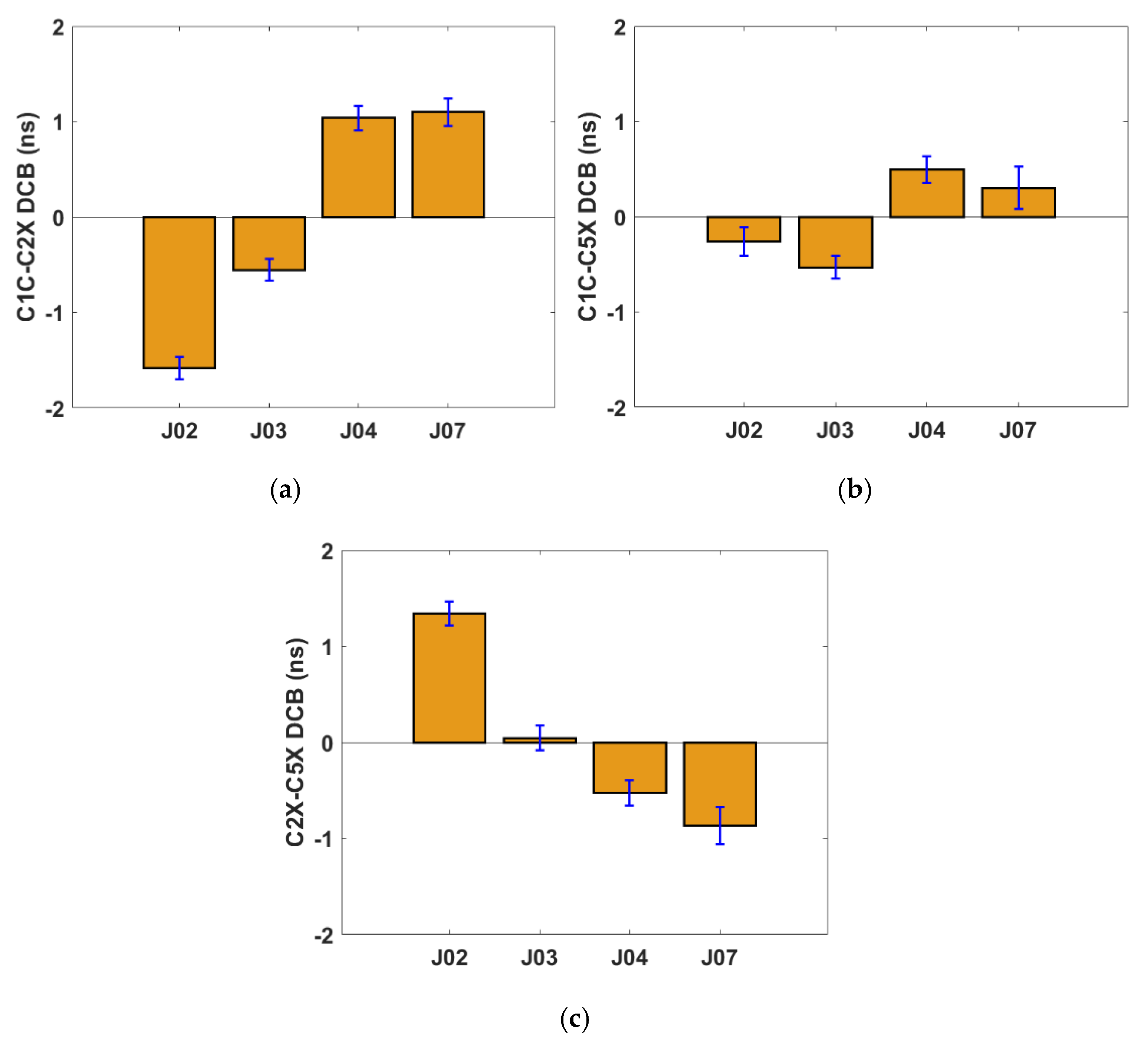
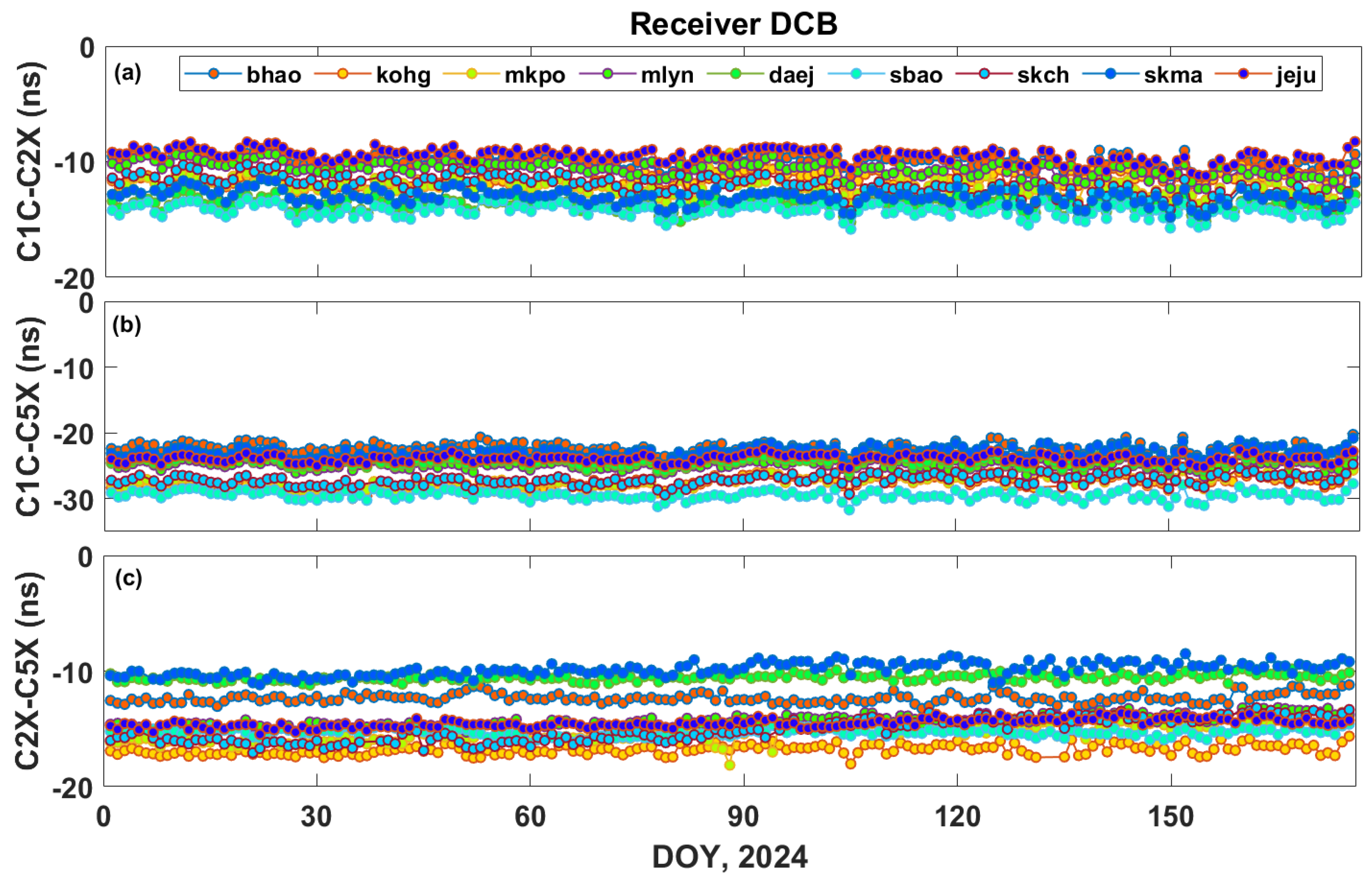
4.1. QZSS Satellite DCB
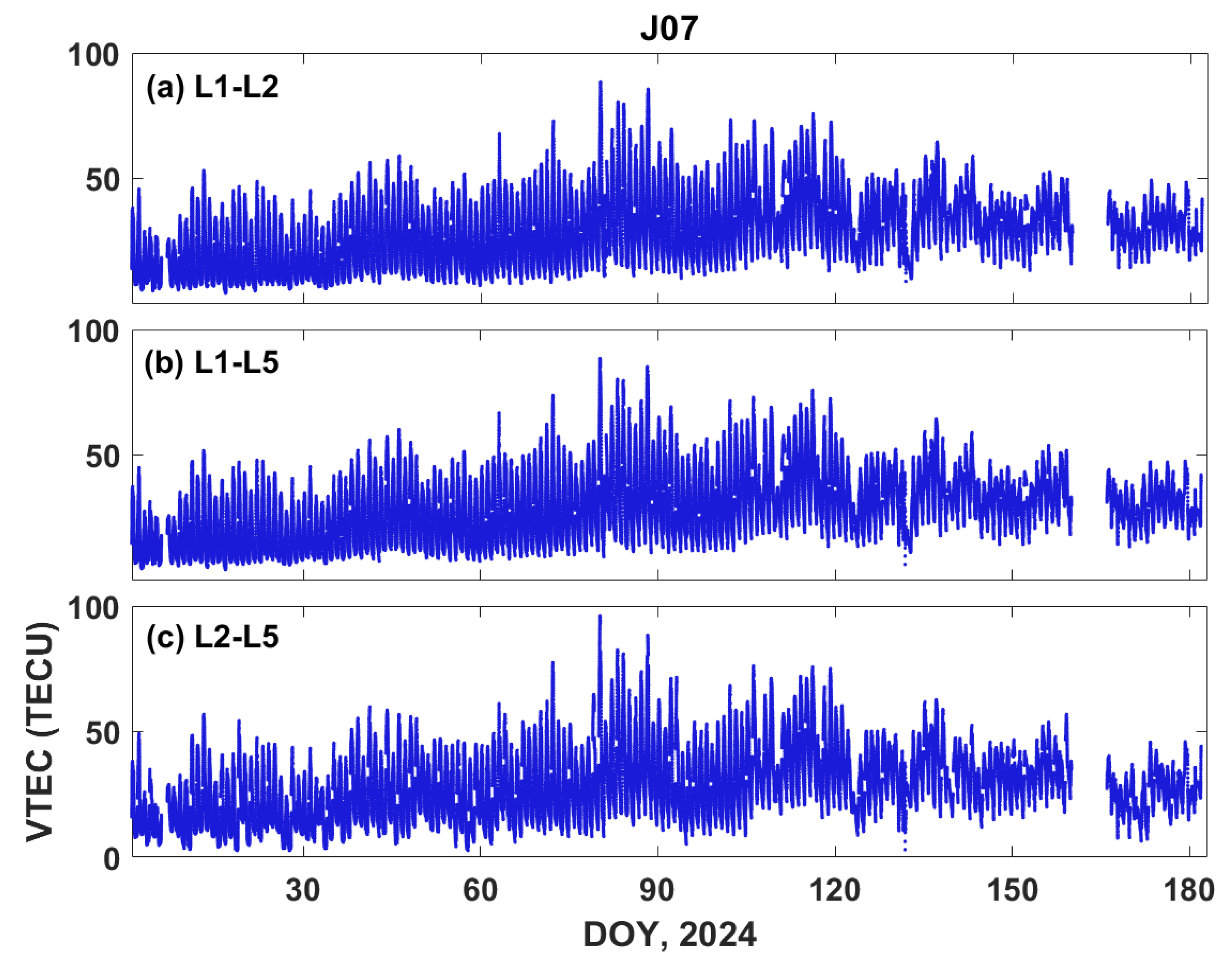
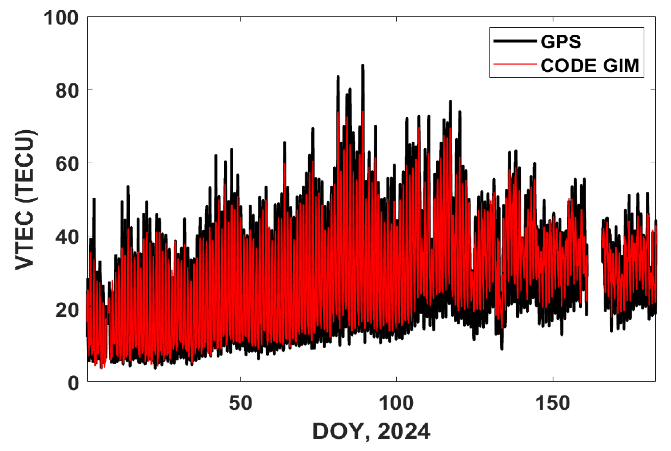
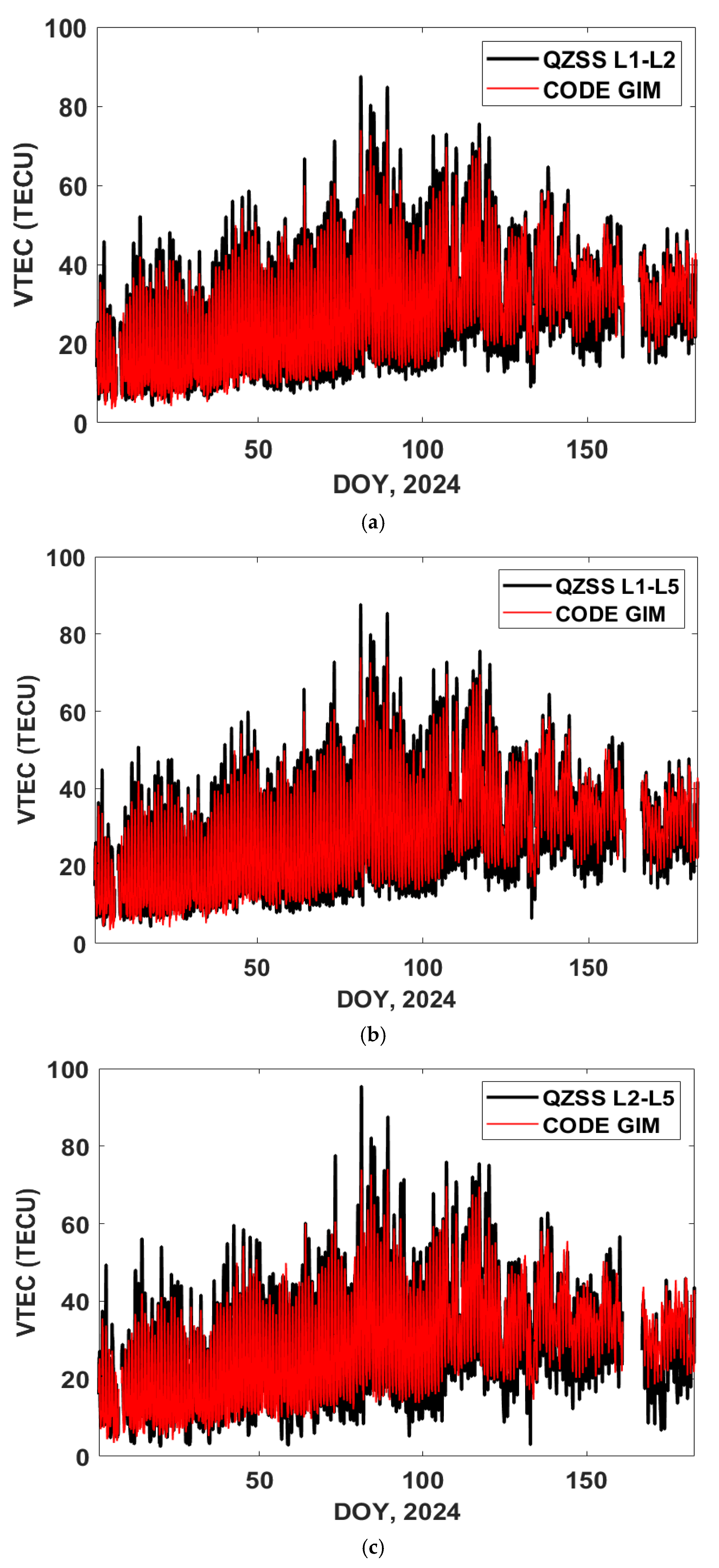
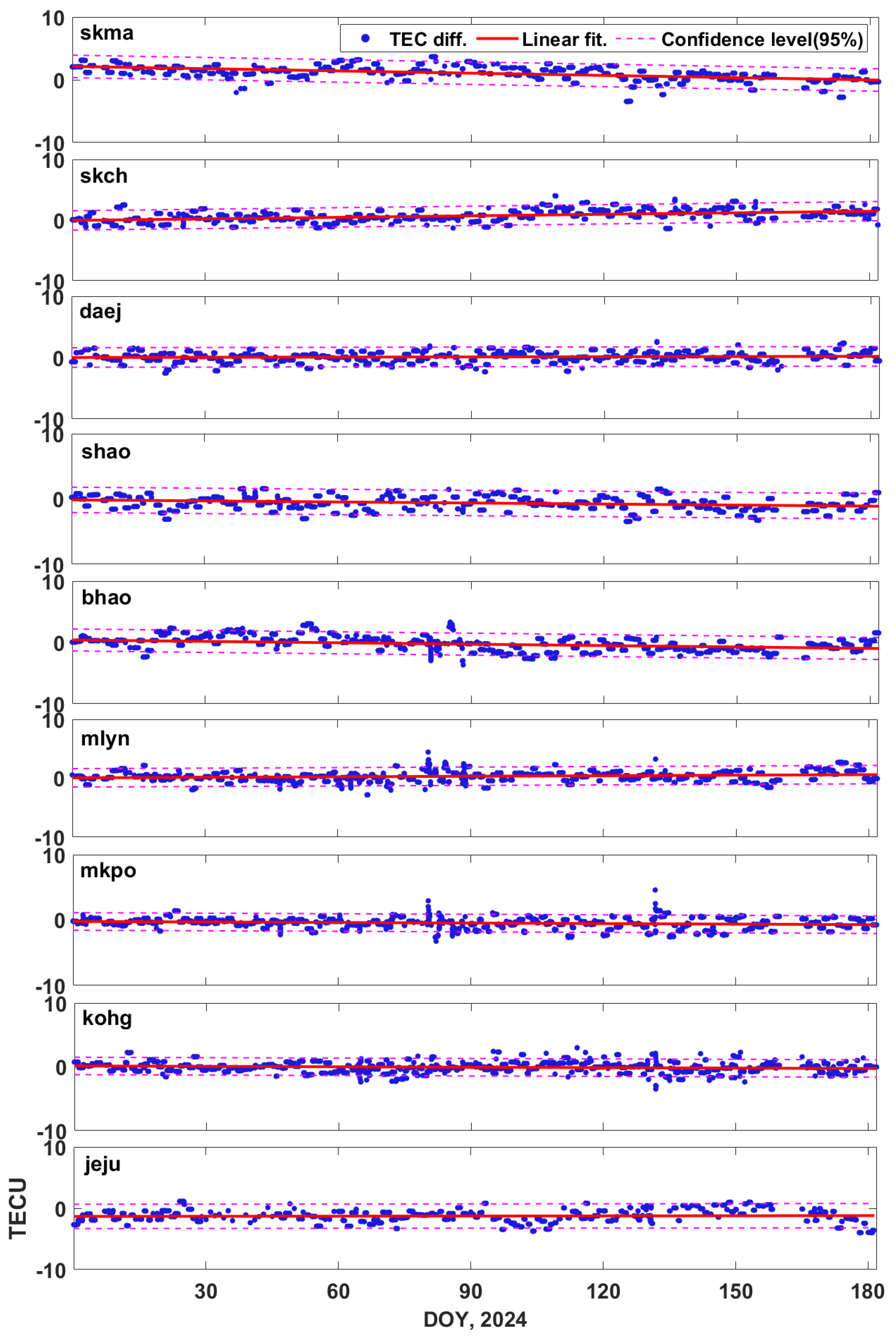
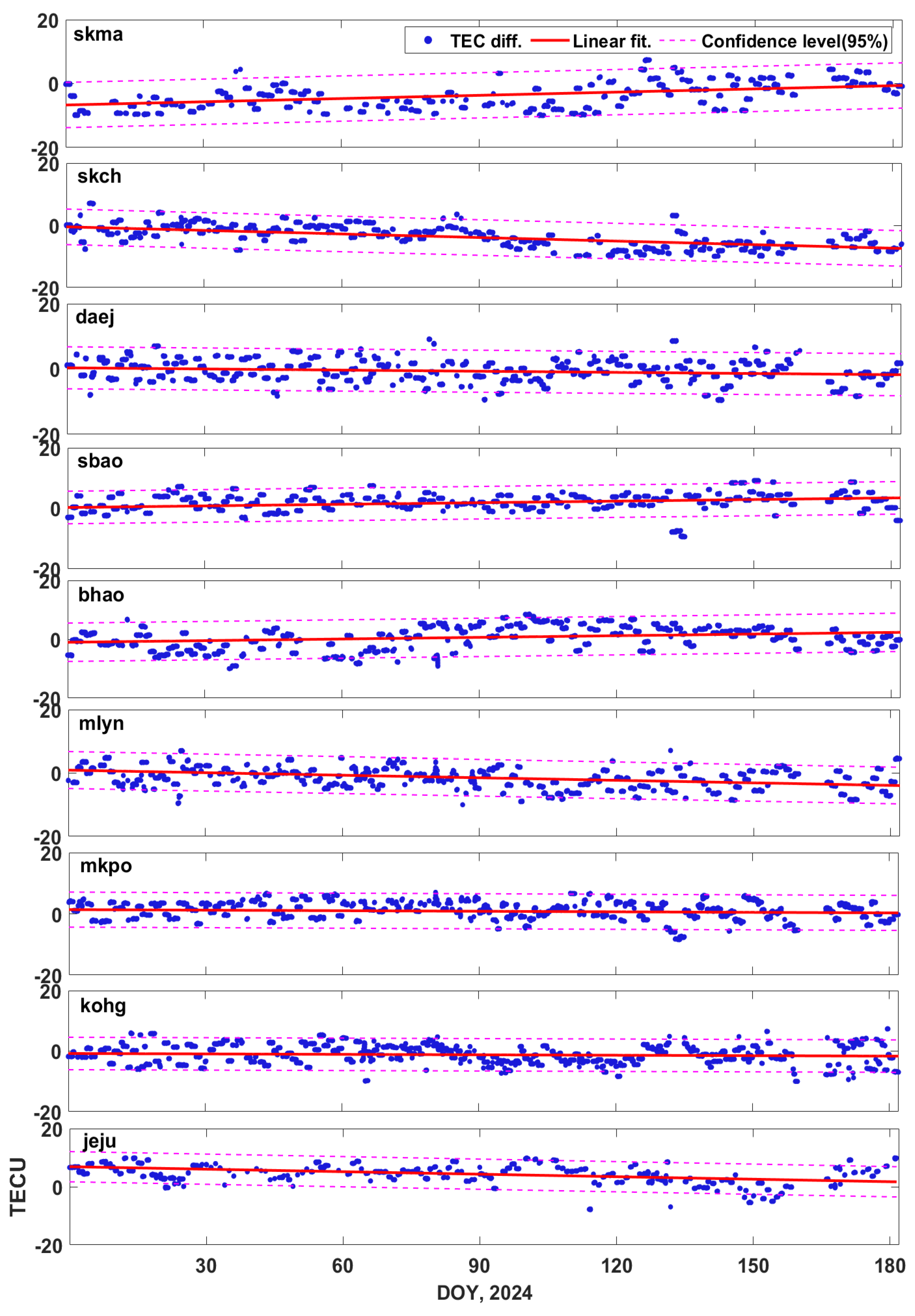
4.2. QZSS TEC
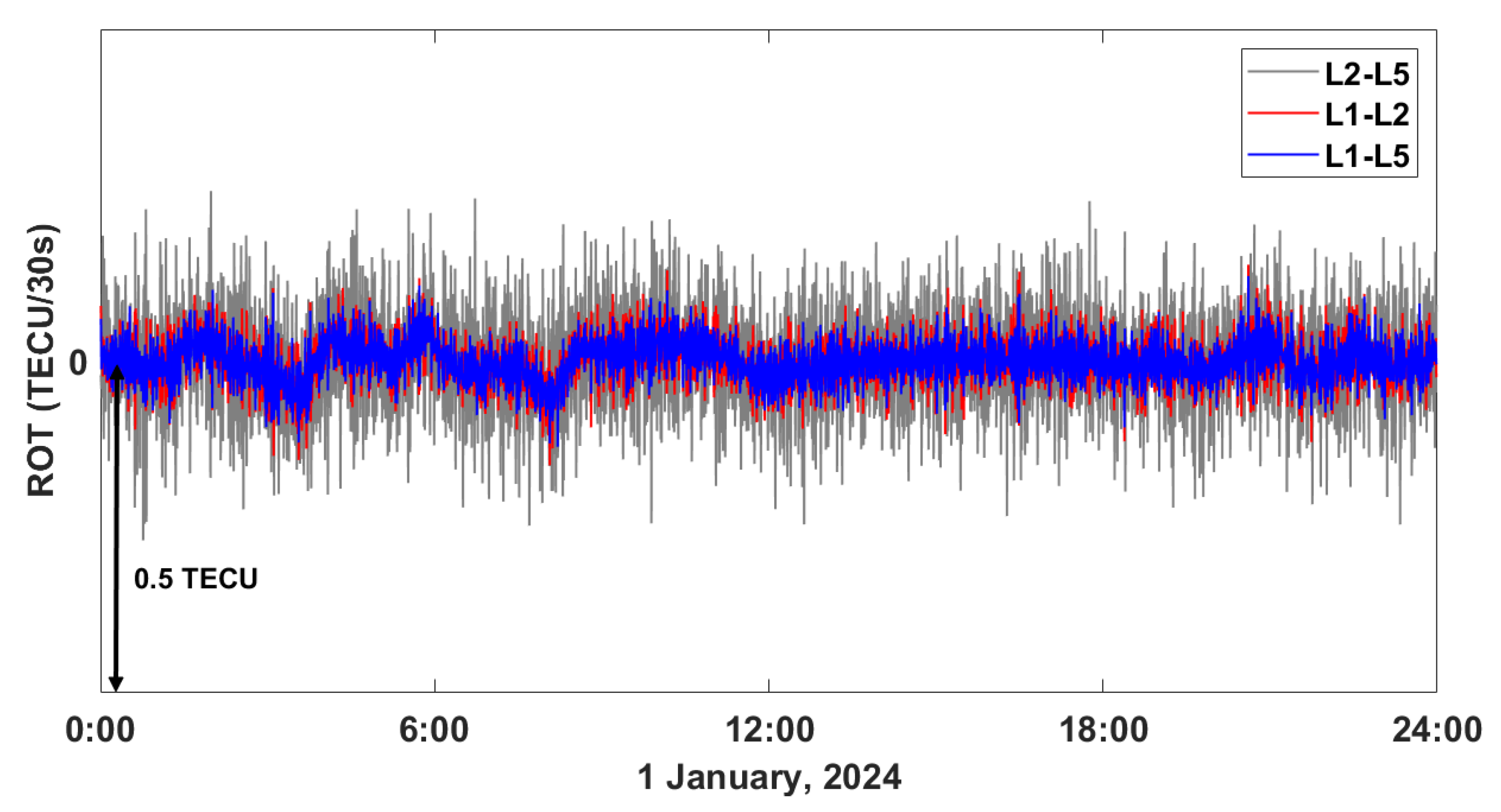
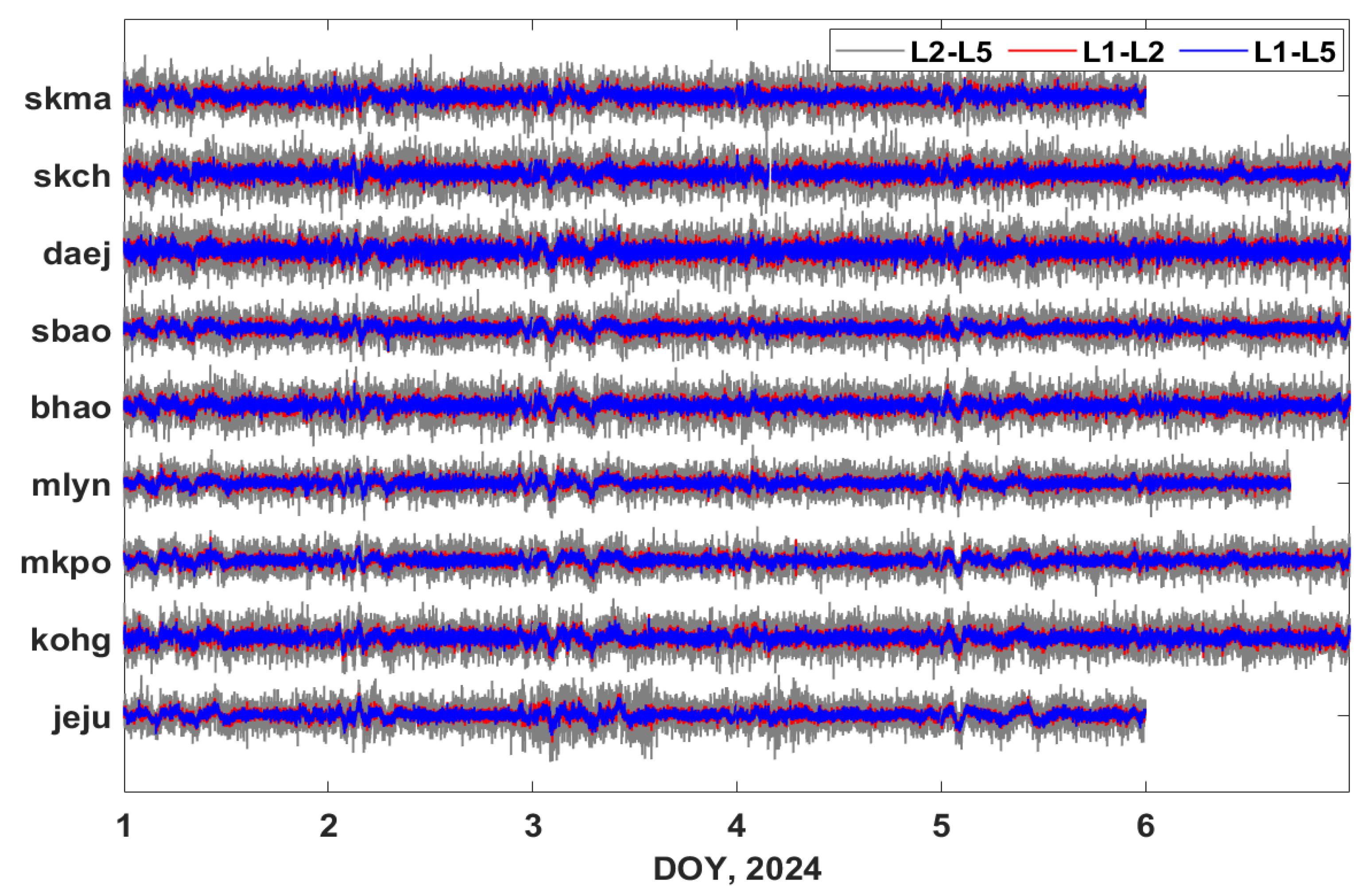
4.3. ROT Analysis
5. Discussion
6. Conclusions
Author Contributions
Funding
Data Availability Statement
Acknowledgments
Conflicts of Interest
References
- Schaer, S.; Beutler, G.; Rothacher, M. Mapping and Predicting the Ionosphere. In Proceedings of the IGS Analysis Center Workshop, Darmstadt, Germany, 9–11 February 1998; pp. 307–318. [Google Scholar]
- Afraimovich, E.L.; Astafyeva, E.I.; Zhivetiev, I.V.; Oinats, A.V.; Yasyukevich, Y.V. Global Electron Content during Solar Cycle 23. Geomagn. Aeron. 2008, 48, 187–200. [Google Scholar] [CrossRef]
- Mannucci, A.J.; Wilson, B.D.; Yuan, D.N.; Ho, C.H.; Lindqwister, U.J.; Runge, T.F. A global mapping technique for GPS-derived ionospheric total electron content measurements. Radio Sci. 1998, 33, 565–582. [Google Scholar] [CrossRef]
- Bilitza, D.; Altadill, D.; Zhang, Y.; Mertens, C.; Truhlik, V.; Richard, P.; Mckinnell, L.-A.; Reinisch, B. The International Reference Ionosphere 2012—A model of international collaboration. J. Space Weather Space Clim. 2014, 4, A07. [Google Scholar] [CrossRef]
- Yilmaz, A.; Akdogan, K.E.; Gurun, M. Regional TEC mapping using neural networks. Radio Sci. 2009, 44, RS3007. [Google Scholar] [CrossRef]
- Chen, J.; Xiong, P.; Wu, H.; Zhang, X.; Feng, J.; Zhang, T. A Multi-Parameter Empirical Fusion Model for Ionospheric TEC in China’s Region. Remote Sens. 2023, 15, 5445. [Google Scholar] [CrossRef]
- Wang, A.; Zhang, Y.; Chen, J.; Wang, H.; Liu, X.; Xu, Y.; Li, J.; Yan, Y. Exploring the Advantages of Multi-GNSS Ionosphere-Weighted Single-Frequency Precise Point Positioning in Regional Ionospheric VTEC Modeling. Remote Sens. 2025, 17, 1104. [Google Scholar] [CrossRef]
- Kee, C.; Parkinson, B.W.; Axelrad, P. Wide Area Differential GPS. Navigation 1991, 38, 123–145. [Google Scholar] [CrossRef]
- Yuan, Y.; Ou, J. A generalized trigonometric series function model for determining ionospheric delay. Prog. Nat. Sci. 2004, 14, 1010–1014. [Google Scholar] [CrossRef]
- Wang, J.; Liu, Y.-R.; Shi, Y.-F. A high accuracy spatial reconstruction method based on surface theory for regional ionospheric TEC prediction. Space Weather 2023, 21, e2023SW003663. [Google Scholar] [CrossRef]
- Oztan, G.; Duman, H.; Alcay, S.; Ogutcu, S.; Ozdemir, B.N. Analysis of Ionospheric VTEC Retrieved from Multi-Instrument Observations. Atmosphere 2024, 15, 697. [Google Scholar] [CrossRef]
- Doğanalp, S.; Köz, İ. Investigating Different Interpolation Methods for High-Accuracy VTEC Analysis in Ionospheric Research. Atmosphere 2024, 15, 986. [Google Scholar] [CrossRef]
- Xu, H.; Chen, X.; Ou, J.; Yuan, Y. Crowdsourcing RTK: A new GNSS positioning framework for building spatial high-resolution atmospheric maps based on massive vehicle GNSS data. Satell. Navig. 2024, 5, 13. [Google Scholar] [CrossRef]
- Petković, D.; Odalović, O.; Nina, A.; Todorović -Drakul, M.; Kolarski, A.; Grekulović, S.; Krstić, S. Development of High-Precision Local and Regional Ionospheric Models Based on Spherical Harmonic Expansion and Global Navigation Satellite System Data in Serbia. Atmosphere 2025, 16, 496. [Google Scholar] [CrossRef]
- Xiong, B.; Li, Y.; Yu, C.; Li, X.; Li, J.; Zhao, B.; Ding, F.; Hu, L.; Wang, Y.; Du, L. Constructing a Regional Ionospheric TEC Model in China with Empirical Orthogonal Function and Dense GNSS Observation. Remote Sens. 2023, 15, 5207. [Google Scholar] [CrossRef]
- Roma, D.; Hernandez, M.; Krankowski, A.; Kotulak, K.; Ghoddousi-Fard, R.; Yuan, Y.; Li, Z.; Zhang, H.; Shi, C.; Wang, C.; et al. Consistency of seven different GNSS global ionospheric mapping techniques during one solar cycle. J. Geod. 2018, 92, 691–706. [Google Scholar] [CrossRef]
- Blewitt, G. An automated editing algorithm for GPS data. Geophys. Res. Lett. 1990, 17, 199. [Google Scholar] [CrossRef]
- Ma, G.; Maruyama, T. Derivation of TEC and estimation of instrumental biases from GEONET in Japan. Ann. Geophys. 2003, 21, 2083–2093. [Google Scholar] [CrossRef]
- Sardón, E.; Rius, A.; Zarraoa, N. Estimation of the transmitter and receiver differential biases and the ionospheric total electron content from Global Positioning System observations. Radio Sci. 1994, 29, 577–586. [Google Scholar] [CrossRef]
- Yuan, Y.; Tscherning, C.; Knudsen, P.; Xu, G.; Ou, J. The ionospheric eclipse factor method (IEFM) and its application to determining the ionospheric delay for GPS. J. Geod. 2008, 82, 1–8. [Google Scholar] [CrossRef]
- Hu, L.; Yue, X.; Ning, B. Development of the Beidou Ionospheric Observation Network in China for space weather monitoring. Space Weather 2017, 15, 974–984. [Google Scholar] [CrossRef]
- Xiong, B.; Wan, W.; Ning, B.; Hu, L.; Ding, F.; Zhao, B.; Li, J. Investigation of mid- and low-latitude ionosphere based on BDS, GLONASS and GPS observations. Chin. J. Geophys. 2014, 57, 3586–3599. (In Chinese) [Google Scholar] [CrossRef]
- Yang, Y.; Xu, Y.; Li, J.; Yang, C. Progress and performance evaluation of BeiDou global navigation satellite system: Data analysis based on BDS-3 demonstration system. Sci. China Earth Sci. 2018, 61, 614–624. [Google Scholar] [CrossRef]
- GPS World. Available online: https://www.gpsworld.com/the-status-of-qzss/ (accessed on 13 December 2024).
- Wang, Q.; Jin, S.; Hu, Y. Estimation of QZSS differential code biases using QZSS/GPS combined observations from MGEX. Adv. Space Res. 2021, 67, 1049–1057. [Google Scholar] [CrossRef]
- Heki, K.; Fujimoto, T. Atmospheric modes excited by the 2021 August eruption of the Fukutoku-Okanoba volcano, Izu–Bonin Arc, observed as harmonic TEC oscillations by QZSS. Earth Planets Space 2022, 74, 27. [Google Scholar] [CrossRef]
- Choi, B.-K.; Sohn, D.-H.; Hong, J.; Lee, W.K. QZSS TEC Estimation and Validation Over South Korea. J. Position. Navig. Timing 2023, 12, 343–348. (In Korean) [Google Scholar] [CrossRef]
- QZSS Technical Documentation. Available online: https://qzss.go.jp/en/technical/satellites/index.html (accessed on 28 March 2025).
- Heki, K. Ionospheric signatures of repeated passages of atmospheric waves by the 2022 Jan. 15 Hunga Tonga-Hunga Ha’apai eruption detected by QZSS-TEC observations in Japan. Earth Planets Space 2022, 74, 112. [Google Scholar] [CrossRef]
- Rama Rao, P.V.S.; Gopi Krishna, S.; Niranjan, K.; Prasad, D.S.V.V.D. Temporal and spatial variations in TEC using simultaneous measurements from the Indian GPS network of receivers during the low solar activity period of 2004–2005. Ann. Geophys. 2006, 24, 3279–3292. [Google Scholar] [CrossRef]
- Klobuchar, J. Design and characteristics of the GPS ionospheric time-delay algorithm for single-frequency users. In Proceedings of the PLANS ‘86 Position Location and Navigation Symposium, Las Vegas, NV, USA, 4–7 November 1986; pp. 280–286. [Google Scholar]
- Klobuchar, J.A. Ionospheric time-delay algorithm for single-frequency GPS users. IEEE Trans. Aerosp. Electron. Syst. 1987, 3, 325–331. [Google Scholar] [CrossRef]
- Yuan, Y.; Wang, N.; Li, Z.; Huo, X. The BeiDou Global Broadcast Ionospheric Delay Correction Model (BDGIM) and Its Preliminary Performance Evaluation Results. Navigation 2019, 66, 55–69. [Google Scholar] [CrossRef]
- Lanyi, G.E.; Roth, T. A comparison of mapped and measured total ionospheric electron content using global positioning system and beacon satellite observations. Radio Sci. 1988, 23, 483–492. [Google Scholar] [CrossRef]
- Sardon, E.; Zarraoa, N. Estimation of the total electron content using GPS data: How stable are the differential satellite and receiver instrumental biases? Radio Sci. 1997, 32, 1899–1910. [Google Scholar] [CrossRef]
- Jakowski, N.; Schlüter, S.; Sardon, E. Total electron content of the ionosphere during the geomagnetic storm on 10 January 1997. J. Atmos. Sol.-Terr. Phys. 1999, 61, 299–307. [Google Scholar] [CrossRef]
- Otsuka, Y.; Ogawa, T.; Saito, A.; Tsugawa, T.; Fukao, S.; Miyazaki, S. A new technique for mapping of total electron content using GPS network in Japan. Earth Planets Space 2002, 54, 63–70. [Google Scholar] [CrossRef]
- Wang, Q.; Zhu, J.; Feng, H. Ionosphere Total Electron Content Modeling and Multi-Type Differential Code Bias Estimation Using Multi-Mode and Multi-Frequency Global Navigation Satellite System Observations. Remote Sens. 2023, 15, 4607. [Google Scholar] [CrossRef]
- Arikan, F.; Erol, C.B.; Arikan, O. Regularized estimation of vertical total electron content from Global Positioning System data for a desired time period. Radio Sci. 2004, 39, RS6012. [Google Scholar] [CrossRef]
- Meza, A. Three Dimensional Ionospheric Models from Earth and Space Based GPS Observations. Ph.D. Thesis, Universidad Nacional de La Plata, Buenos Aires, Argentina, 1999. [Google Scholar]
- Zhang, D.H.; Zhang, W.; Li, Q.; Shi, L.Q.; Xiao, Z. Accuracy Analysis of the GPS Instrumental Bias Estimated from Observations in Middle and Low Latitudes. Ann. Geophys. 2010, 28, 1571–1580. [Google Scholar] [CrossRef]
- Schaer, S.; Beutler, G.; Mervart, L.; Rothacher, M.; Wild, U. Global and regional ionosphere models using the GPS double difference phase observable. In Proceedings of the IGS Workshop “Special Topics and New Directions”, Potsdam, Germany, 15–18 May 1995; pp. 77–92. [Google Scholar]
- Wang, Y.; Yue, D.; Wang, H.; Ma, H.; Liu, Z.; Yue, C. Comprehensive Analysis of BDS/GNSS Differential Code Bias and Compatibility Performance. Remote Sens. 2024, 16, 4217. [Google Scholar] [CrossRef]
- Pi, X.; Mannucci, A.J.; Lindqwister, U.J.; Ho, C.M. Monitoring of global ionospheric irregularities using the worldwide GPS network. Geophys. Res. Lett. 1997, 24, 2283–2286. [Google Scholar] [CrossRef]
- Tiwari, R.; Bhattacharya, S.; Purohit, P.K.; Gwal, A.K. Effect of TEC variation on GPS precise point at low latitude. Open Atmos. Sci. J. 2009, 3, 1–12. [Google Scholar] [CrossRef]
- Yao, Y.; Liu, L.; Kong, J.; Zhai, C. Analysis of the global ionospheric disturbances of the March 2015 great storm. J. Geophys. Res. Space Phys. 2016, 121, 12157–12170. [Google Scholar] [CrossRef]
- Warnant, R. Reliability of the TEC computed using GPS measurements—The problem of hardware biases. Acta Geod. Geophys. Hung. 1997, 32, 451–459. [Google Scholar] [CrossRef]
- Coster, A.; Williams, J.; Weatherwax, A.; Rideout, W.; Herne, D. Accuracy of GPS total electron content: GPS receiver bias temperature dependence. Radio Sci. 2013, 48, 190–196. [Google Scholar] [CrossRef]
- Yasyukevich, Y.V.; Mylnikova, A.A.; Kunitsyn, V.E.; Padokhin, A.M. Influence of GPS/GLONASS differential code biases on the determination accuracy of the absolute total electron content in the ionosphere. Geomag. Aeron. 2015, 55, 763–769. [Google Scholar] [CrossRef]
- Choi, B.K.; Lee, S.J. The influence of grounding on GPS receiver differential code biases. Adv. Space Res. 2018, 62, 457–463. [Google Scholar] [CrossRef]
- Hernández-Pajares, M.; Juan, J.M.; Sanz, J.; Orús, R.; Garcia-Rigo, A.; Feltens, J.; Komjathy, A.; Schaer, S.C.; Krankowski, A. The IGS VTEC maps: A reliable source of ionospheric information since 1998. J. Geod. 2009, 83, 263–275. [Google Scholar] [CrossRef]


| Site Name | Geographic Latitude (Degrees) | Geographic Longitude (Degrees) |
|---|---|---|
| skch | 38.25°N | 128.56°E |
| skma | 37.49°N | 126.91°E |
| sbao | 36.93°N | 128.45°E |
| daej | 36.39°N | 127.37°E |
| bhao | 36.16°N | 128.97°E |
| mlyn | 35.49°N | 128.74°E |
| mkpo | 34.81°N | 126.38°E |
| kohg | 34.45°N | 127.51°E |
| jeju | 33.28°N | 126.46°E |
| Signal | Observation Types |
|---|---|
| L1 | C1C, L1C, C1X, L1X, C1Z, L1Z |
| L2 | C2X, L2X |
| L5 | C5X, L5X |
| PRN | Signal Combination | Average Value (ns) | RMS Value (ns) |
|---|---|---|---|
| J02 | C1C-C2X | −1.58 | 0.11 |
| C1C-C5X | −0.26 | 0.14 | |
| C2X-C5X | 1.34 | 0.12 | |
| J03 | C1C-C2X | −0.55 | 0.11 |
| C1C-C5X | −0.53 | 0.12 | |
| C2X-C5X | 0.04 | 0.12 | |
| J04 | C1C-C2X | 1.03 | 0.12 |
| C1C-C5X | 0.49 | 0.14 | |
| C2X-C5X | −0.52 | 0.13 | |
| J07 | C1C-C2X | 1.10 | 0.14 |
| C1C-C5X | 0.30 | 0.22 | |
| C2X-C5X | −0.86 | 0.19 |
| Site Name | Signals | RMS Value (TECU) |
|---|---|---|
| L1-L2 | 0.034 | |
| skma | L1-L5 | 0.028 |
| L2-L5 | 0.073 | |
| L1-L2 | 0.036 | |
| skch | L1-L5 | 0.030 |
| L2-L5 | 0.079 | |
| L1-L2 | 0.039 | |
| daej | L1-L5 | 0.033 |
| L2-L5 | 0.083 | |
| L1-L2 | 0.029 | |
| sbao | L1-L5 | 0.025 |
| L2-L5 | 0.064 | |
| L1-L2 | 0.033 | |
| bhao | L1-L5 | 0.028 |
| L2-L5 | 0.073 | |
| L1-L2 | 0.028 | |
| mlyn | L1-L5 | 0.025 |
| L2-L5 | 0.059 | |
| L1-L2 | 0.028 | |
| mkpo | L1-L5 | 0.025 |
| L2-L5 | 0.059 | |
| L1-L2 | 0.035 | |
| kohg | L1-L5 | 0.029 |
| L2-L5 | 0.072 | |
| L1-L2 | 0.028 | |
| jeju | L1-L5 | 0.025 |
| L2-L5 | 0.059 |
Disclaimer/Publisher’s Note: The statements, opinions and data contained in all publications are solely those of the individual author(s) and contributor(s) and not of MDPI and/or the editor(s). MDPI and/or the editor(s) disclaim responsibility for any injury to people or property resulting from any ideas, methods, instructions or products referred to in the content. |
© 2025 by the authors. Licensee MDPI, Basel, Switzerland. This article is an open access article distributed under the terms and conditions of the Creative Commons Attribution (CC BY) license (https://creativecommons.org/licenses/by/4.0/).
Share and Cite
Choi, B.-K.; Sohn, D.-H.; Hong, J.; Chung, J.-K.; Park, K.-D.; Lee, H.K.; Kim, J.; Choi, H.H. Ionospheric TEC and ROT Analysis with Signal Combinations of QZSS Satellites in the Korean Peninsula. Remote Sens. 2025, 17, 1945. https://doi.org/10.3390/rs17111945
Choi B-K, Sohn D-H, Hong J, Chung J-K, Park K-D, Lee HK, Kim J, Choi HH. Ionospheric TEC and ROT Analysis with Signal Combinations of QZSS Satellites in the Korean Peninsula. Remote Sensing. 2025; 17(11):1945. https://doi.org/10.3390/rs17111945
Chicago/Turabian StyleChoi, Byung-Kyu, Dong-Hyo Sohn, Junseok Hong, Jong-Kyun Chung, Kwan-Dong Park, Hyung Keun Lee, Jeongrae Kim, and Heon Ho Choi. 2025. "Ionospheric TEC and ROT Analysis with Signal Combinations of QZSS Satellites in the Korean Peninsula" Remote Sensing 17, no. 11: 1945. https://doi.org/10.3390/rs17111945
APA StyleChoi, B.-K., Sohn, D.-H., Hong, J., Chung, J.-K., Park, K.-D., Lee, H. K., Kim, J., & Choi, H. H. (2025). Ionospheric TEC and ROT Analysis with Signal Combinations of QZSS Satellites in the Korean Peninsula. Remote Sensing, 17(11), 1945. https://doi.org/10.3390/rs17111945