Using an Area-Weighted Loss Function to Address Class Imbalance in Deep Learning-Based Mapping of Small Water Bodies in a Low-Latitude Region

Abstract

Recent advances in very high resolution PlanetScope imagery and deep-learning techniques have enabled effective mapping of small water bodies (SWBs), including ponds and ditches. SWBs typically occupy a minor proportion of remote-sensing imagery. This creates significant class imbalance that introduces bias in trained models. Most existing deep-learning approaches fail to adequately address this imbalance. Such an imbalance introduces bias in trained models. Most existing deep-learning approaches fail to adequately address the inter-class (water vs. non-water) and intra-class (SWBs vs. large water bodies) simultaneously. Consequently, they show poor detection of SWBs. To address these challenges, we propose an area-based weighted binary cross-entropy (AWBCE) loss function. AWBCE dynamically weights water bodies according to their size during model training. We evaluated our approach through large-scale SWB mapping in the middle and east of Hubei Province, China. The models were trained on 14,509 manually annotated PlanetScope image patches (512 × 512 pixels each). We implemented the AWBCE loss function in State-of-the-Art segmentation models (UNet, DeepLabV3+, HRNet, LANet, UNetFormer, and LETNet) and evaluated them using overall accuracy, F1-score, intersection over union, and Matthews correlation coefficient as accuracy metrics. The AWBCE loss function consistently improved performance, achieving better boundary accuracy and higher scores across all metrics. Quantitative and visual comparisons demonstrated AWBCE’s superiority over other imbalance-focused loss functions (weighted BCE, Dice, and Focal losses). These findings emphasize the importance of specialized approaches for comprehensive SWB mapping using high-resolution PlanetScope imagery in low-latitude regions.

1. Introduction

Lakes, reservoirs, and ponds are key components of the Earth’s indispensable water resources and play major roles in environmental processes such as global biogeochemical cycles and greenhouse gas emissions. Unlike large lakes and reservoirs, small water bodies (SWBs, usually <10,000 m²) play critical roles in regional agricultural irrigation but also contribute more CO₂ and CH₄ per unit area than large lakes [1]. Compared with the SWBs of thaw ponds that are distributed in high latitudes, including Alaska and Siberia [2,3,4], a large number of SWBs, such as aquaculture ponds and small farm reservoirs, are prevalent in many low-latitude regions, where they are used for water storage for irrigation and aquaculture [5,6,7].

Satellite remote sensing has enabled wall-to-wall mapping of SWBs from space [2,8,9,10,11,12]. Landsat imagery with a spatial resolution of typically 30 m has been used to map small lakes larger than 30,000 m² globally [13]. However, the results are affected by the mixed pixel problem due to the relatively coarse resolution [14,15,16]. Sentinel-2 has enabled the mapping of SWBs at 10 m resolution [8,17], but it is still challenging to detect SWBs smaller than 1000 m² (i.e., approximately ten Sentinel-2 pixels) [18,19]. By contrast, the development of very high resolution remote sensing has enabled the mapping of SWBs at a spatial resolution finer than 10 m. In particular, mapping SWBs has been applicable with the use of Chinese Gaofen [20], Kanopus-V [4], and Google Earth imagery [5,21]. PlanetScope imagery from the Planet Labs’ constellation of satellites provides a great opportunity for mapping SWBs at approximately 3 m resolution and daily frequency [22]. The unsupervised thresholding methods of OTSU segmentation have been applied to PlanetScope for mapping small on-farm reservoirs [6,23]. However, they are based on the assumption that water and non-water have a bimodal distribution in the water index band. Without requiring a specific distribution of water and non-water in the water index band, the data-driven deep learning-based models, which are popular in recent semantic segmentation, have been applied to map SWBs from PlanetScope imagery in recent years [3].

Although deep-learning models show strong potential in mapping SWBs from very high resolution imagery, most fail to address class imbalance. This imbalance occurs both between classes (water vs. non-water, since water covers <2% of Earth’s surface) and within the water class itself, where small SWBs dominate in count but contribute little to total water area, while large lakes may be less abundant but contain a larger proportion of the total water area. Deep-learning models trained on imbalanced datasets exhibit a bias toward majority classes, as their optimization for overall accuracy often compromises the detection of minority classes, such as SWBs [24,25,26]. Consequently, without addressing class imbalance, these models typically identify only a subset of SWBs and frequently fail to detect those smaller than 100 m² [3,4,5,27].

Various methods have been proposed to address class imbalance in machine and deep learning, particularly in binary classification. These approaches fall into two categories: data-level and algorithmic-level methods [28]. At the data level, common techniques include oversampling (duplicating minority-class samples) and undersampling (reducing majority-class samples). For example, Li et al. [29] addressed class imbalance by oversampling water pixels tenfold to equilibrate water/non-water distributions. However, oversampling SWB samples may introduce overfitting and amplify label noise, whereas random undersampling of background pixels risks eliminating informative features (e.g., shadows and roads) that could otherwise help distinguish them from actual water bodies [24]. Additionally, the oversampling and undersampling methods may lead to a class distribution shift [30]. Chawla et al. [31] proposed a Synthetic Minority Oversampling Technique (SMOTE) which generates the synthetic minority data by interpolating neighboring data points in the feature space, but it could result in overgeneralization with high variance [32,33]. Generative adversarial network (GAN)-based oversampling, which generates realistic minority samples [34,35], has been applied in remote sensing (e.g., forest mapping [36] and sea-ice segmentation [37]). However, the GAN-based oversampling methods are computationally intensive and may fail to capture the data distribution information and generate similar SWB samples [35,36].

At the algorithmic level, modifying loss functions is a common approach to address class imbalance by assigning higher weights to minority classes. Deep-learning semantic segmentation employs several loss functions to address class imbalance. The weighted binary cross-entropy (WBCE) loss assigns higher weights to minority classes [38], and it has been successfully applied in urban water extraction [39] and glacial lake mapping [27]. However, its effectiveness diminishes with extreme class imbalances (>10:1 ratio) [30,40], a situation commonly encountered in SWB mapping, where SWBs occupy only a tiny fraction of the image. Focal loss extends cross-entropy (CE) and binary cross-entropy (BCE) losses through class-frequency weighting [41], demonstrating success in medical imaging [42] and water segmentation [43]. However, it remains sensitive to label noise in the SWB training dataset, which may result in a vanishing gradient during backpropagation in SWB mapping [44,45]. Unlike Focal loss, Dice loss is developed to improve the intersection over union (IoU) [46]. Dice loss shows promise in sea-ice segmentation [47], but it emphasizes foreground regions, possibly leading to training instability and causing instability with small targets [48]. This limitation poses a particular challenge for the accurate detection and segmentation of SWBs, as they are represented by very few pixels in the image and are easily overlooked. While hybrid approaches combining Dice with BCE/WBCE/Focal losses exist [49,50,51,52], they often increase model complexity [53]. Crucially, all the aforementioned weighted loss functions are designed to address the inter-class imbalance problem, but none of them address the intra-class imbalance problem, to the best of our knowledge, thus possibly limiting their effectiveness in mapping SWBs.

While deep learning has proven effective for mapping thaw ponds in high-latitude regions using PlanetScope imagery [3], its application for SWB mapping in low-latitude areas (<33° from the equator) remains unexplored. The SWBs in the low-latitude region exhibit distinct characteristics compared to those in other regions. Due to the region’s flat terrain, dense river network, and extensive agricultural activities, SWBs in the low-latitude region are typically more fragmented, shallow, and temporally dynamic. These water bodies often exhibit significant seasonal variability in regard to both spatial and spectral properties, influenced by irrigation practices and land-use changes. This differs from SWBs in mountainous and high-latitude regions, which tend to be more stable, less fragmented, and more strongly influenced by topography or groundwater availability. Such differences present unique challenges for remote sensing-based mapping of SWBs in this region. This data-driven approach requires extensive training samples, particularly challenging for low-latitude SWBs, which exhibit greater spectral variability due to diverse types (aquaculture ponds, reservoirs, and ditches) and varying water properties (suspended solids, turbidity, and chlorophyll) [54,55]. Unlike Arctic ponds that typically appear dark blue/green, low-latitude water bodies show wider color variations influenced by human activities (farming, fishing, and tourism). Current benchmark datasets like GID [56,57], while useful for general water mapping, inadequately represent low-latitude SWBs—often merging adjacent ponds or excluding smaller water bodies.

This study aims to fill the knowledge gap in using deep-learning models for wall-to-wall mapping of SWBs from PlanetScope in a relatively low-latitude region. To generate representative training samples of SWBs in low latitudes, a PlanetScope-based SWB dataset was built. The dataset comprises 14,509 image patches, each containing 512 × 512 pixels, of PlanetScope imagery. Water bodies were manually digitized in the image patches, and various SWBs, including ponds, ditches, small reservoirs, and small lakes, were included in the dataset. In addition, to simultaneously account for the inter-class and intra-class imbalance problems, the area-based WBCE (AWBCE) loss was proposed by highlighting the weights of the minor proportion of water compared with non-water and the minor proportion of small SWBs compared with large lakes. In this study, not only was water assigned a higher weight than non-water, but SWBs were assigned a higher weight than the relatively larger lakes and rivers, thus causing the model to focus more on water and particularly on SWBs to improve performance. The model with the proposed loss function was compared with several State-of-the-Art deep-learning models with other loss functions for alleviating the class-imbalance problem, and it was validated in a small area experiment, using an unmanned aerial vehicle (UAV), and a large area experiment (~93,925 km²), using Google Earth imagery for validation.

2. Study Area and Data

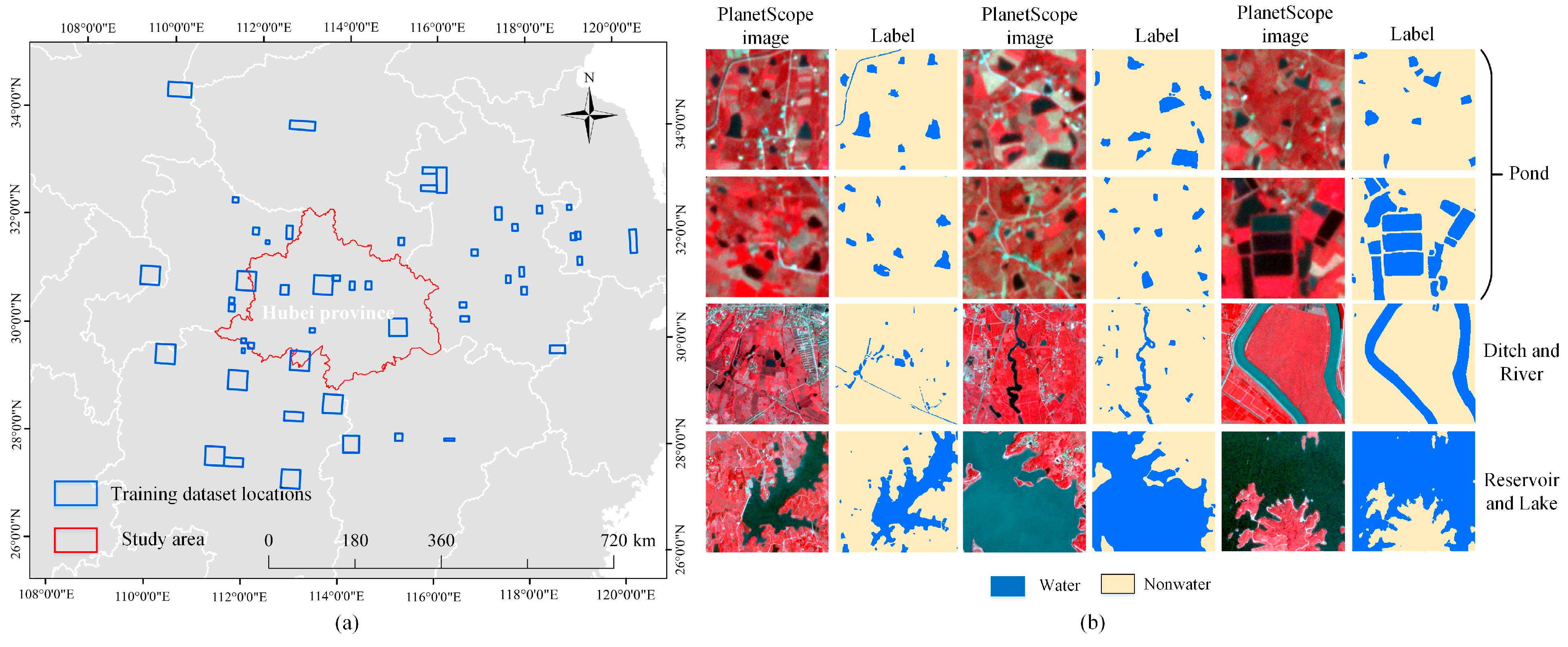
2.1. Study Area

The study area is located in the middle and east of Hubei Province, China (Figure 1a). This area is mainly composed of plains with an elevation of approximately 150 m. The study site contains the Jianghan Plain, an alluvial plain of the Yangtze and Han Rivers. The study site contains various water bodies, including large lakes, small reservoirs, aquaculture ponds, ditches, and small ponds.

2.2. Data

2.2.1. PlanetScope

The PlanetScope Analytic Ortho Scene Product (Level 3B) acquired from the 3rd generation of PlanetScope sensors was used. Each PlanetScope image has a size of approximately 24 km × 7 km. The PlanetScope images comprise four spectral bands, including blue (465–515 nm), green (547–583 nm), red (650–680 nm), and near-infrared (650–680 nm) with a spatial resolution of approximately 3 m. We restricted our analysis to the four PlanetScope bands to maintain compatibility across all historical and current imagery over the 5-year period [58].

2.2.2. Construction of Training Dataset for Deep-Learning Models

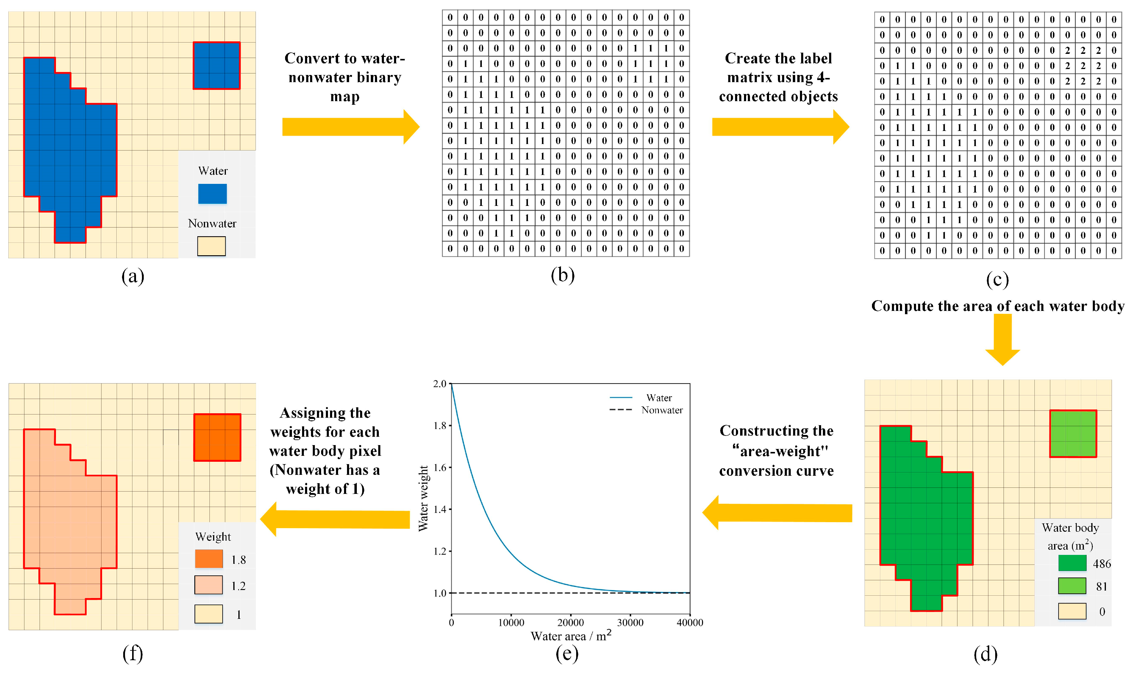
A PlanetScope-based water body dataset, including a large number of PlanetScope image patches and the corresponding water label maps, was constructed. The locations of the PlanetScope imagery are shown in Figure 1a. The acquisition times of the PlanetScope images were mainly from July 2017 to November 2021, including different seasons. The water bodies were then manually delineated according to PlanetScope, and the labels were visually checked by experts. The dataset includes 405,091 water bodies that represent various types, including small ponds, ditches, rivers, lakes, and reservoirs (Figure 1b). In the dataset, the total areas of water bodies and non-water are approximately 2.7 × 10⁹ and 3.1 × 10¹⁰ m², showing an imbalance in class proportions between water and non-water (i.e., an inter-class imbalance). For water labels, a total of 21,544 water bodies are smaller than 100 m² and cover an area of 759,740 m² (0.03% in total water area); 181,504 water bodies are in the size ranging from 100 to 1000 m², with an area of 94,472,412 m² (3.47% in total water area); 181,935 water bodies are in the size ranging 1000 to 10,000 m², with an area of 532,280,459 m² (19.56% in total water area); and 20,108 water bodies are larger than 10,000 m², with an area of 2,094,041,936 m² (76.94% in total water area). SWBs are numerous but take a small fraction of the total water area, showing a serious intra-class imbalance problem.

The PlanetScope imagery and the corresponding water maps were split into non-overlapping patches with 512 × 512 pixel size. A total of 14,509 patches of images were created. Of these patches, 85% of the patches (12,332 patches) were randomly selected for training the deep-learning models, and the remaining 15% (2177 patches) of patches were used as the validation dataset [59]. Additionally, to avoid overfitting and enlarge the number of training samples for the deep-learning models, data augmentation operations were conducted to enhance the number of training data. In particular, the patches within the training dataset were randomly rotated by one of the three angles (90°, 180°, or 270°), and a total of 24,664 patches were finally generated for model training.

3. Methods

The loss function, also known as the cost function, is a function that maps an event or values representing the cost associated with the event, and it has been used in various fields, including deep learning. It is widely utilized to gauge the disparity between true values and predictions during the training of supervised deep-learning models. The loss function is typically applied in the output layer of deep-learning models and is therefore independent of the specifics of the deep-learning model itself. During the training process, the calculated loss from the current network is fed back into the network, prompting corresponding updates to the network parameters. In this study, the loss function is designed that be used with the State-of-the-Art semantic segmentation models used for water mapping.

BCE loss is a commonly used loss function for image segmentation in deep-learning models. BCE loss was used to quantify the difference between the predicted probability and the true probability as Equation (1):

$$\mathrm{BCE} Loss=-{\displaystyle \frac{1}{N}}{\sum }_{i=1}^N\left[p_i·\log \left(q_i\right)+(1-p_i)·\mathrm{l}\mathrm{o}\mathrm{g}(1-q_i)\right]$$

(1)

where $p_i$ is the reference label of the i-th pixel, $p_i$ = 0 indicates negative class (non-water in this study), $p_i$ = 1 indicates positive class (water in this study), $q_i$ is the predicted probability belonging to the water class of the i-th pixel, and N is the total number of pixels in an image. Water and non-water classes are given equal weights in Equation (1). In water mapping, since most pixels are non-water pixels, which are usually denoted as negative examples, and only a few pixels belong to water, denoted as positive examples, training deep-learning models with BCE loss makes it difficult to extract accurate water bodies because non-water pixels are dominant in number.

The classic weighted BCE (WBCE) loss aims to reduce the class imbalance problem in BCE [60]. The classic WBCE loss assigns higher weights for the minority class as follows:

$$WBCE Loss=-{\displaystyle \frac{1}{N}}{\sum }_{i=1}^N\left[{W·p}_i·\mathit{log}\left(q_i\right)+(1-p_i)·\mathrm{l}\mathrm{o}\mathrm{g}(1-q_i)\right]$$

(2)

where $W$ is the weight for the positive class of water. In general, $W$ > 1 is set to increase the impact of the positive class on the loss function. Although WBCE can alleviate the class imbalance to some extent, it usually adopts a fixed value of $W$. In other words, it is regardless of intra-class imbalance in SWB mapping.

In this study, the proposed AWBCE, which is constructed based on WBCE, is designed to give different values of $W$ for different water bodies according to their sizes. In general, SWBs contain a relatively small proportion of water pixels, while large lakes and reservoirs tend to have a relatively high proportion of water pixels. Taking this intra-class imbalance into account, AWBCE assigns higher weights to smaller water bodies compared to relatively larger ones:

$$AWBCE Loss=-{\displaystyle \frac{1}{N}}{\sum }_{i=1}^N\left[{W_i·p}_i·\log \left(q_i\right)+\left(1-p_i\right)·\log \left(1-q_i\right)\right]$$

(3)

where $W_i$ is the weight for the ith water pixel as the positive class. The flowchart of the calculation of $W_i$ is shown in Figure 2.

Figure 2a is a water–non-water label image for training. Since the label images are in raster format, in order to extract the area of each water body, we first determine which water body each pixel belongs to. This is fulfilled based on the connected components of water pixels using MATLAB’s ‘bwlabel’ function. In particular, a binary image with ‘1’ indicating the water pixel and ‘0’ indicating the non-water pixel is created (Figure 2b). Then, a label matrix (with water labels indicating different water body objects) using 4 connected objects is built (Figure 2c). The number of PlanetScope pixels that belongs to each water body is thus calculated, and the area of the k-th water body is calculated in Equation (4) and Figure 2d:

$${Area}_k={NP}_k\times s^2$$

(4)

where ${NP}_k$ is the number of pixels in the k-th water body; and $s$ is the spatial resolution of PlanetScope, i.e., $s$ = 3 m. The unit of ${Area}_k$ is measured in square meters.

Once the area of each water body is calculated, weights are assigned to different water bodies based on their respective areas. For the i-th water pixel in the training dataset, the corresponding weight that accounts for intra-class imbalance, i.e., $W_i^{intra}$, is calculated as follows:

$$\begin{gathered} W_i^{intra}=exp\left({\displaystyle \frac{-{Area}_k}{\alpha }}\right)·z_{ik} \\ {z}_{ik}=\left\{\begin{array}{cc}1& if pixel i belongs to the k^{th} water body\\ 0& otherwise\end{array}\right. \end{gathered}$$

(5)

where $\alpha$ is an adjustable parameter. Based on Equation (5), the weights of different water pixels can be assigned using an exponential decay function according to the sizes of the corresponding water bodies to which the pixels belong. Pixels belonging to smaller water bodies are assigned higher weights than those associated with larger water bodies, resulting in greater loss contributions from SWB pixels during model training. This, in turn, encourages the model to pay more attention to these SWBs. As a result, the model could learn more representative features of SWBs to improve its capability to map SWBs.

The value of $W_i^{intra}$ ranges from 0 to 1 in Equation (5). In order to give a relatively higher weight of water body and a relatively lower value for non-water to account for the inter-class imbalance, the final weight of the i-th water pixel, i.e., $W_i,$ is calculated as follows:

$${W_i=W}_i^{intra}+1=exp\left({\displaystyle \frac{-{Area}_k}{\alpha }}\right)·z_{ik}+1$$

(6)

The variation in the weight, $W_i$, with the variance of parameter $\alpha$ in Equation (6), which controls the relationship between the area of water bodies and the corresponding weight of these water bodies, is shown in Figure 3. Previous studies show that deep learning and machine learning can map water bodies of about larger than 30,000 m² with high accuracy from high-resolution PlanetScope [3,6,23]. Thus, these water bodies are referred to as well-classified examples that are assigned with $W_i$ of close to 1, similar to the non-water samples, in this study. In contrast, SWBs are more challenging to accurately map and are thus regarded as hard samples and assigned relatively higher weights. This approach proposes the AWBCE loss to focus the deep-learning model on learning from hard examples of SWBs, thereby enhancing the relative loss for these instances while reducing the relative loss for well-classified examples of larger water bodies and non-water samples.

Once the weights of all water pixels were calculated, the proposed AWBCE was constructed. In the proposed AWBCE loss, the water pixels were assigned higher weights than non-water pixels to alleviate the inter-class imbalance problem, and the water bodies that were smaller in size were assigned higher weights than those that were relatively larger to alleviate the intra-class imbalance problem.

4. Experiments

The proposed AWBCE loss was assessed in two experiments. The first experiment adopted the study site with a small area of approximately 10 km² (Figure 4). In the second experiment, the study site located in the central and eastern Hubei province with an area of 93,925 km² was selected (Figure 1 and Figure 5). This region contained a large number of SWBs of different kinds.

4.1. Small Area Experiment Using UAV for Validation

This experiment used a small subset of PlanetScope imagery for prediction. The PlanetScope image acquired on 9 June 2023 was used as the input data of models (Figure 4a). The study area covers an area of approximately 10 km² that is located within the area in Figure 1. Here, to assess the performance of the outputs generated from the PlanetScope imagery, UAV imagery with 2.5 cm spatial resolution was adopted. The UAV RGB images were collected from 12 June 2023 to 15 June 2023, temporally close to the PlanetScope image. The UAV data were collected using a DJI Phantom 4 real-time kinematic (RTK) for validation. All the UAV images are mosaicked in Figure 4b. The mosaicked UAV image was manually interpreted into a binary water map used for validation. A total of 481 water bodies were interpreted in this area, including 122 water bodies smaller than 100 m², 347 water bodies of 100–10,000 m², and 12 water bodies larger than 10,000 m².

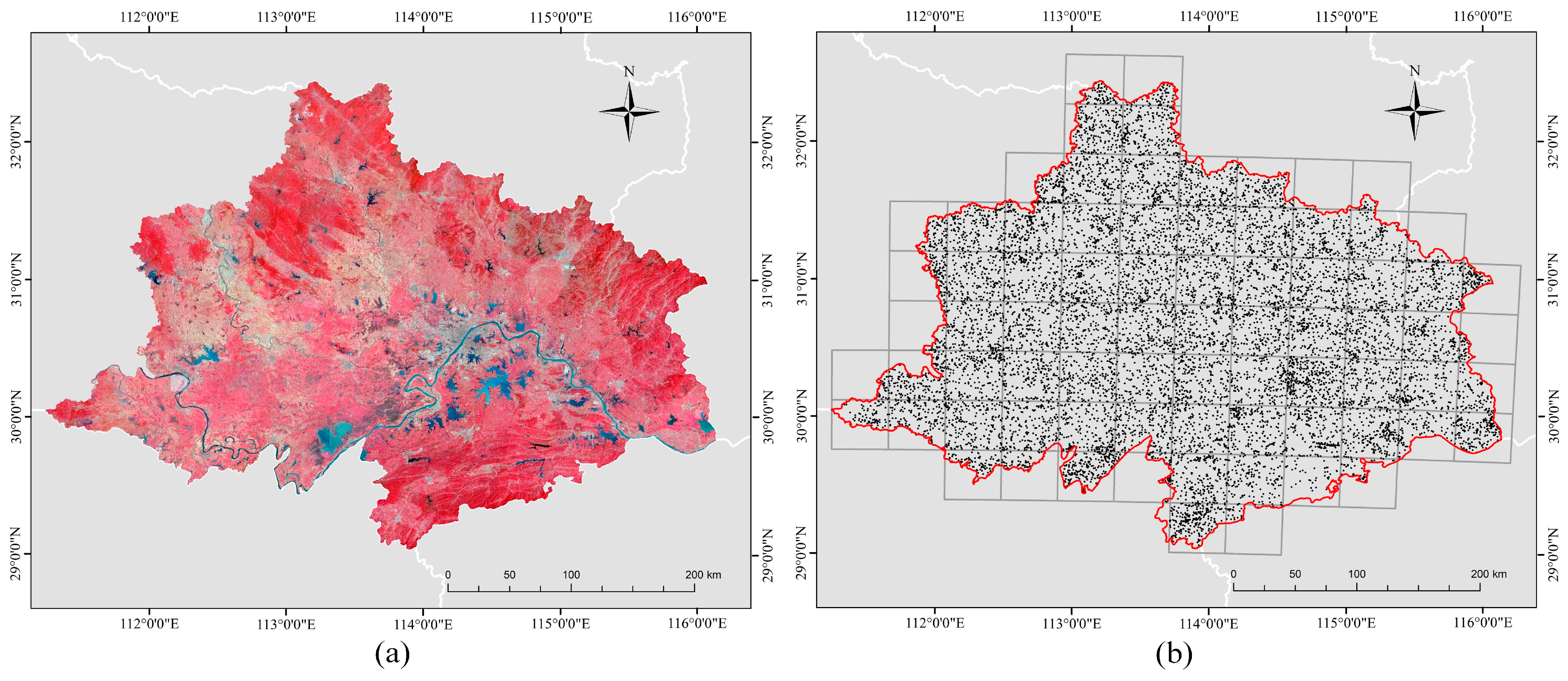
4.2. Large Area Experiment Using Random Sample Points from Google Earth for Validation

This experiment utilized the entire study area depicted in Figure 1 to map SWBs. In total, 77 PlanetScope images covering the study area were used. The images were mainly acquired in September 2022. All the images were cloud-free, and mosaicked, as shown in Figure 5a. Randomly sampled points were used for validation (Figure 5b). The study region was divided into 77 grids, with each grid containing an area of 40 km × 40 km. In each grid, 200 validation samples, including about 100 water pixel labels and 100 non-water pixel labels, were randomly selected for validation. If only parts of a grid belong to the study area, then the number of sample pixels decreased correspondingly. A total of 12,518 samples were used for validation. The labels of each sample point were interpreted by experts. The details of the data in the two experiments are shown in

Table 1. The detailed information about the data used in this paper.

	Training	Validation	Small Area Experiment		Large Area Experiment
			Input	Water Mask	Input	Water Mask
Number of image patches	24,664	2177	1	1	1	-
Image size (in pixels)	512 × 512	512 × 512	1007 × 1043	Approximately 120,000 × 125,000	120,840 × 125,160	12,518 random sample points
Spatial resolution	3 m	3 m	3 m	0.025 m	3 m	<1 m
Data source	PlanetScope	PlanetScope	PlanetScope	UAV	PlanetScope	Google Earth image

.

4.3. Comparators and Model Parameter Settings

Several State-of-the-Art deep-learning semantic models, including DeepLabV3+ [61], High-Resolution Net (HRNet) [62], Local Attention Network (LANet) [63], UNet [64], UNetFormer [65], and LETNet [66], were used in water mapping. UNet employs a symmetric encoder–decoder architecture that is widely used in image segmentation. DeepLabV3+ contains the atrous spatial pyramid pooling module to learn multi-scale features with dilated convolutions. HRNet extracts multi-scale features with many parallel high-to-low resolution streams throughout the model. LANet is a representative model that embeds localized attention mechanisms into the semantic segmentation task. UNetFormer and LETNet are hybrid CNN and Transformer architecture models, which could take both the local features and global context features into account, and they have been widely used in semantic segmentation tasks.

For each model, the modes with the traditional BCE loss without considering class imbalance (i.e., UNet, DeepLabV3+, HRNet, LANet, UNetFormer, and LETNet) and with the proposed AWBCE loss that considered the class imbalance (i.e., UNet_AWBCE DeepLabV3+_AWBCE, HRNet_AWBCE, LANet_AWBCE, UNetFormer_AWBCE, and LETNet_AWBCE) were compared.

In addition, since several loss functions have addressed the class imbalance problem, the proposed AWBCE loss that considered both inter- and intra-class imbalance was compared with State-of-the-Art loss functions designed for class imbalance problems, including the WBCE loss [60]; Dice loss [46]; Focal loss [41]; and the combined loss functions, including DiceBCE loss (combination of Dice and BCE loss) [67] and DiceFocal loss (combination of Dice and Focal loss) [68]. All the loss functions were validated with the UNet model as the base model, which was used in recent SWBs mapping models with PlanetScope [3,21,69]. All the models were trained with the same parameters.

All the models were trained with the gradient backpropagation algorithm [70] with the PyTorch 1.10.0 deep-learning framework based on NVIDIA 3090Ti GPU with 24 GB of RAM and cuDNN 10.0 for acceleration. The Adam optimization algorithm [71] for gradient descent was used. The batch size, initial learning rate, and weight decay were 8, 1 × 10⁻⁴, and 1 × 10⁻⁵, respectively. Hyper-parameter $\alpha$ was set as 6000 within the AWBCE loss. The impact of different $\alpha$ values is discussed in the Discussion section. In the training stage, the model’s performance is primarily influenced by random factors [72]. In order to obtain a robust result, a fixed random seed was used in the training stage, which allows the stochastic components of the model to remain consistent. We trained each model for 200 epochs on the training datasets. The model achieving the highest accuracy on the validation dataset was selected to map water bodies of the study area.

4.4. Accuracy Assessment

Six metrics of classification accuracy, overall accuracy (OA), User’s Accuracy (UA) for water bodies, Producer’s Accuracy (PA) for water bodies, F1-score (F1), Intersection over Union (IoU), and Matthews correlation coefficient (MCC), were used to quantify the results of different models. OA, UA, PA, F1, IoU, and MCC are calculated as follows:

$$OA=S_d/n$$

(7)

$$UA=X_{ij}/X_{\ast j}$$

(8)

$$PA=X_{ij}/X_{i\ast }$$

(9)

where $S_d$ is the number of pixels that are correctly predicted, $n$ is the total number of pixels, $X_{ij}$ is the number of water pixels that is correctly predicted, $X_{\ast j}$ is the number of pixels that are predicted as water in the prediction map, and $X_{i\ast }$ is the number of water pixels in the reference map.

$$F1=2TP/(2TP+FN+FP)$$

(10)

$$IoU=TP/(TP+FN+FP)$$

(11)

$$MCC=(TP\times TN-FN\times FP)/\left(\left(TP+FP\right)\times \left(TP+FN\right)\times \left(TN+FP\right)\times \left(TN+FN\right)\right)$$

(12)

where TP, TN, FP, and FN represent the numbers of pixels that are true positives (i.e., water correctly predicted as water), true negatives (i.e., non-water correctly predicted as non-water), false positives (i.e., non-water incorrectly predicted as water), and false negatives (i.e., water incorrectly predicted as non-water), respectively.

The IoU for each SWB, (i.e., IoU_pSWB), is also computed to assess the performance of deep learning in mapping SWBs of different sizes:

$${\mathrm{I}\mathrm{o}\mathrm{U}}_{\mathrm{p}\mathrm{S}\mathrm{W}\mathrm{B}}={\displaystyle \frac{area of overlap}{area of union}}$$

(13)

IoU_pSWB ranges from 0 to 1, where 0 indicates no match for the water body in the predicted and labeled images, and 1 indicates a perfect match between the predicted and labeled images.

5. Results

5.1. Result of Small Area Experiment Using UAV for Validation

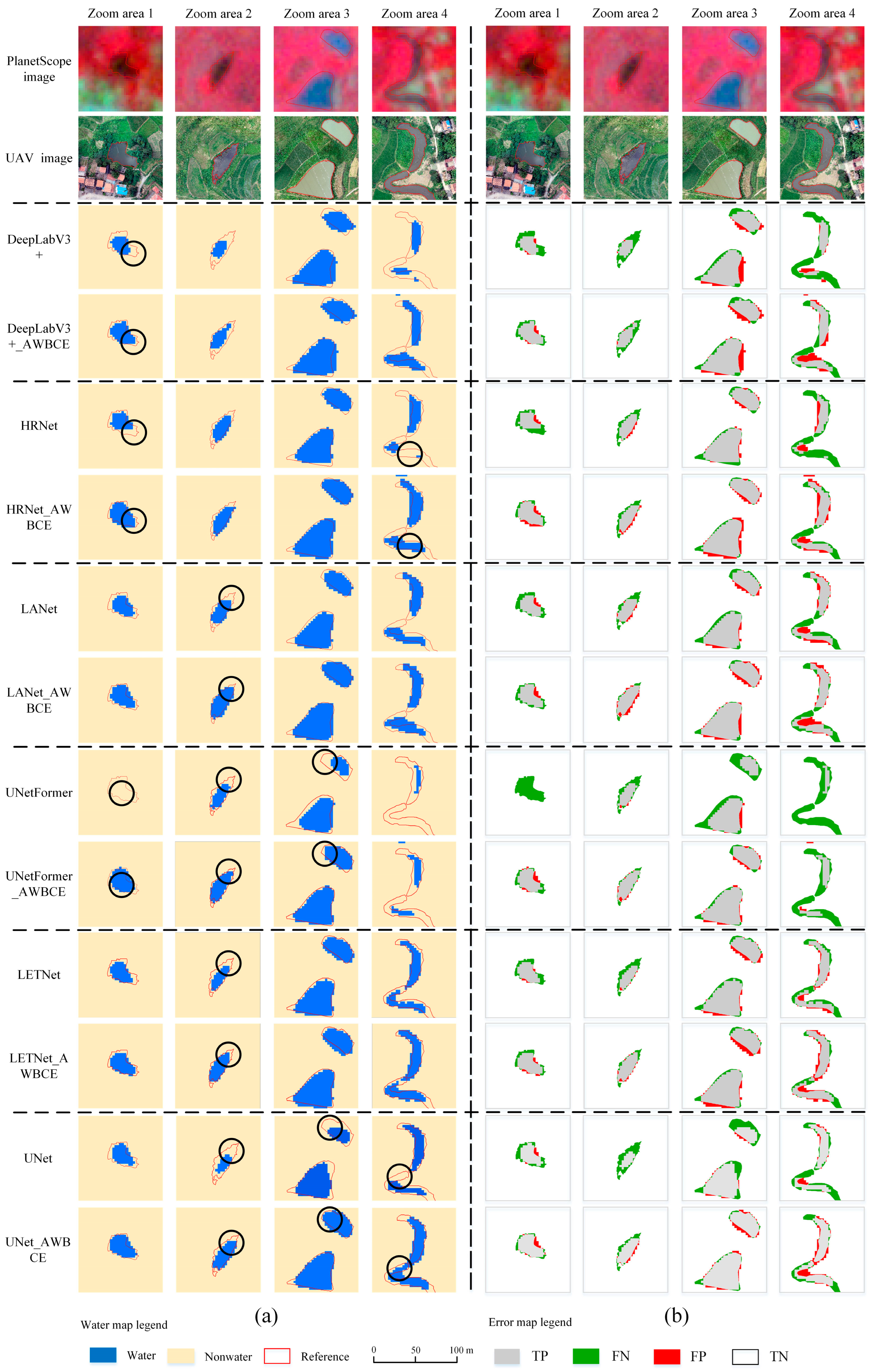
5.1.1. Results of Different Deep-Learning Models with Classic BCE Loss and with the Proposed AWBCE Loss in the Small Area Experiment

The visual comparison between deep-learning models without considering the class imbalance problem (DeepLabV3+, HRNet, LANet, UNetFormer, LETNet, and UNet) and deep-learning models with the proposed AWBCE loss (DeepLabV3+_AWBCE, HRNet_AWBCE, LANet_AWBCE, UNetFormer_AWBCE, LETNet_AWBCE, and UNet_AWBCE) in four zoom areas is shown in Figure 6. In general, models with AWBCE loss mapped more water pixels than those models with BCE loss in all of these zoom areas, such as those highlighted with black circles in Figure 6a. In addition, the SWB boundaries were mapped from the proposed AWBCE loss that better matched the reference boundary, as highlighted in red lines in the water maps in Figure 6a. The main reason was that the AWBCE loss assigned higher weights for water pixels, especially for small ponds, which contributed to more loss in training deep-learning models. With the increase in the size of the SWBs, all the deep-learning models could predict most parts of the SWBs, and the predicted boundary of SWBs from the models using AWBCE better matched the reference boundary in red lines in the zoom areas. It was also found that the deep-learning models with BCE loss usually mapped the linear ditch with disconnected shapes, while the models with the proposed AWBCE loss mapped the linear object with a more connected shape in zoom area 4 in Figure 6a. Among the different models using the AWBCE loss, LETNet_AWBCE and UNet_AWBCE predicted SWBs that were more similar to the reference than other comparators in the zoom areas in Figure 6. In the error maps in Figure 6b, water was incorrectly predicted as non-water (FN, highlighted with green color) and non-water was incorrectly predicted as water (FP, highlighted with red color). In general, the models using AWBCE loss generated fewer FN pixels in green color in the error map than those using BCE loss without considering the class imbalance problem, showing that more water pixels were correctly labeled using the proposed AWBCE loss.

Table 2. The accuracies of the different models in the small area experiment using UAV for validation. The higher accuracy values are highlighted in bold.

Models	OA (%)	UA (%)	PA (%)	F1	IoU	MCC
DeepLabV3+	97.9	91.2	81.7	0.862	0.757	0.852
DeepLabV3+_AWBCE	98.0	89.7	84.6	0.871	0.771	0.861
HRNet	98.0	91.6	82.9	0.870	0.770	0.861
HRNet_AWBCE	98.1	88.1	88.7	0.884	0.792	0.874
LANet	98.0	89.3	85.1	0.872	0.772	0.861
LANet_AWBCE	98.3	89.9	88.4	0.892	0.804	0.882
UNetFormer	98.1	94.8	81.1	0.874	0.776	0.867
UNetFormer_AWBCE	98.2	88.9	88.6	0.888	0.798	0.878
LETNet	98.0	92.0	82.1	0.868	0.766	0.859
LETNet_AWBCE	98.3	90.8	87.5	0.891	0.804	0.882
UNet	98.2	94.3	82.8	0.882	0.789	0.874
UNet_AWBCE	98.4	93.0	86.5	0.896	0.812	0.888

shows the quantitative accuracies from different models. Compared with deep-learning models without considering class imbalance, the models addressing class imbalance with the proposed AWBCE loss generated higher accuracy on all the metrics except UA. This was in accordance with Figure 6, in which the models with the AWBCE loss mapped more water pixels, resulting in a decrease in omission error and an increase in commission error and leading to a higher PA but lower UA than deep-learning models with BCE loss. For instance, UNet_AWBCE increased OA, PA, F1, IoU, and MCC by 0.2%, 3.7%, 0.014, 0.023, and 0.014 compared with UNet. UNet_AWBCE generated the highest OA, PA, F1, IoU, and MCC among different methods. We noticed that UNet with the proposed AWBCE outperformed UNetFormer and LETNet with the proposed AWBCE loss. The main reason is that both UNetFormer and LETNet are Transformer-based models, while Transformer architectures typically rely on vast datasets to effectively capture long-range dependencies and rich contextual information. However, in SWB mapping, training data could be limited, and Transformer-based models are prone to overfitting and may underperform compared to simpler architectures of UNet. In contrast, UNet is simple to train and tends to be more robust in learning settings with limited samples [73].

The accuracies of SWBs of different sizes were analyzed based on the metric of IoU_pSWB (the IoU per SWB) in Figure 7. The IoU_pSWB values from different models were lower than 0.01 when the sizes of water bodies were smaller than 100 m², showing that deep-learning models had difficulties detecting SWBs smaller than 100 m². When the SWBs were larger than 100 m² but smaller than 10,000 m², DeepLabV3+_AWBCE, HRNet_AWBCE, LANet_AWBCE, UNetFormer_AWBCE, LETNet_AWBCE, and UNet_AWBCE increased the IoU_pSWB values by 0.028, 0.006, 0.029, 0.035, 0.041, and 0.026 compared with DeepLabV3+, HRNet, LANet, UNetFormer, LETNet, and UNet, respectively, showing that AWBCE loss outperformed classic BCE loss.

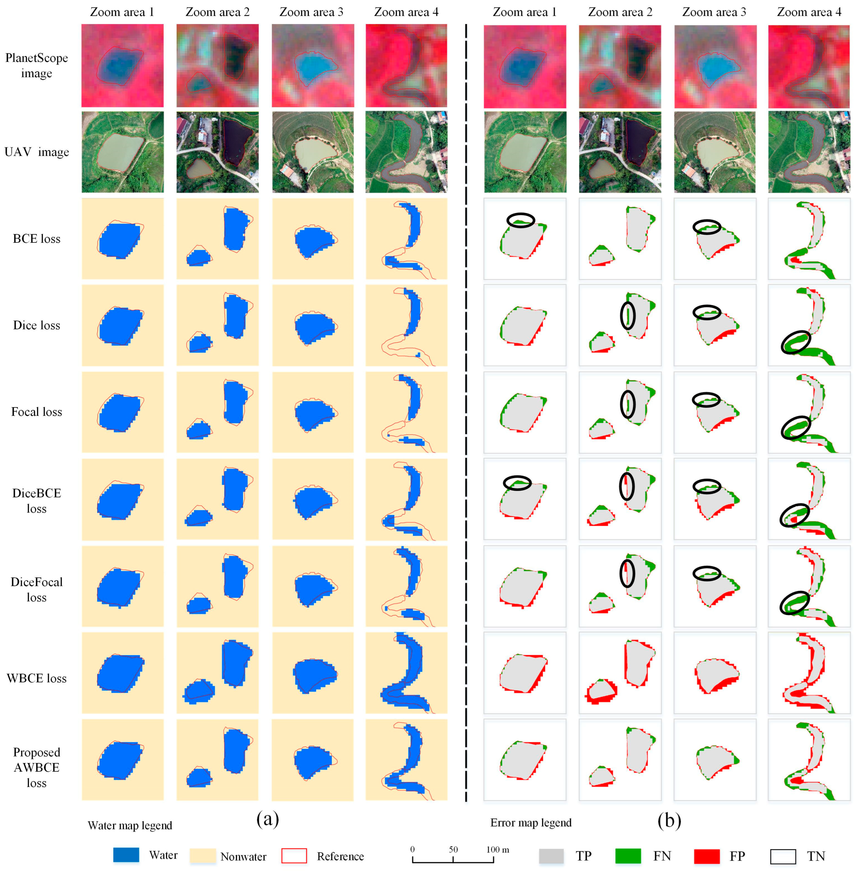
5.1.2. Comparison of Different Loss Functions for Addressing the Class Imbalance Problem in the Small Area Experiment

The visual comparisons of the models using different loss functions for addressing the class imbalance problem are shown in Figure 8. All the models adopted UNet as the base model because UNet was used in recent SWB mapping with PlanetScope studies [3], and it generated relatively higher accuracies than other models in

Table 3. The accuracies of UNet model with different loss functions in the small area experiment using UAV for validation. The highest accuracy values are highlighted in bold.

Models	OA (%)	UA (%)	PA (%)	F1	IoU	MCC
BCE loss	98.2	94.3	82.8	0.882	0.789	0.874
Dice loss	98.2	92.9	84.1	0.883	0.790	0.875
Focal loss	98.3	95.0	83.4	0.888	0.799	0.882
DiceBCE loss	98.2	91.8	85.0	0.883	0.790	0.874
DiceFocal loss	98.3	92.3	85.4	0.887	0.797	0.879
WBCE loss	98.0	83.6	93.0	0.880	0.786	0.871
Proposed AWBCE loss	98.4	93.0	86.5	0.896	0.812	0.888

. The models using WBCE loss predicted more water pixels than other models in the water map, but they generated more FP pixels (non-water incorrectly predicted as water in red color) in the error map, showing an overestimation of the minority class (i.e., water class in this study). This was because WBCE loss, which reweights the samples simply according to the pixel numbers, tended to incorrectly predict the majority class of non-water as the minority class of water [30]. In the predicted water maps, the maps generated from the models using the proposed AWBCE loss better matched the water boundary, such as in zoom areas 2 and 4 in Figure 8a. The models with the BCE loss, Dice loss, Focal loss, DiceBCE loss, and DiceFocal loss generated more FN pixels (water incorrectly predicted as non-water, highlighted in green color) than the model with proposed AWBCE loss in all the zoom areas, such as those highlighted in green and red color with the black ellipses in the error map in Figure 8b.

In Table 3, the model using Focal loss generated the highest UA values, but it generated the lowest PA values (except for the model using BCE without considering the class imbalance problem). It can be explained in Figure 8b that the model using Focal loss generated more FN pixels (water incorrectly predicted as non-water in green color in the error map). The model using WBCE loss achieved the highest PA, but it predicted the lowest UA which aligns with Figure 8b, as it generated more FP pixels (non-water incorrectly predicted as water). Compared with the model using BCE loss without considering the imbalance problem, the improvement in OA, F1, IoU, and MCC was not obvious for the models with the traditional Dice loss, Focal loss, DiceBCE loss, and DiceFocal loss. In contrast, the models using the proposed AWBCE loss had the highest OA, F1, IoU, and MCC values of 98.4%, 0.896, 0.812, and 0.888, respectively. This result showed the importance of addressing both the inter- and intra-class imbalance problem in SWB mapping.

In Figure 9, for SWBs that were larger than 100 m² but smaller than 10,000 m², the model using the proposed AWBCE loss increased the IoU_pSWB values by 0.026, 0.025, 0.011, and 0.02, 0.015, and 0.015, respectively, compared with the models using BCE loss, Dice loss, Focal loss, DiceBCE loss, DiceFocal loss, and WBCE loss, revealing the advantage of AWBCE loss in mapping SWBs.

5.2. Large Area Experiment

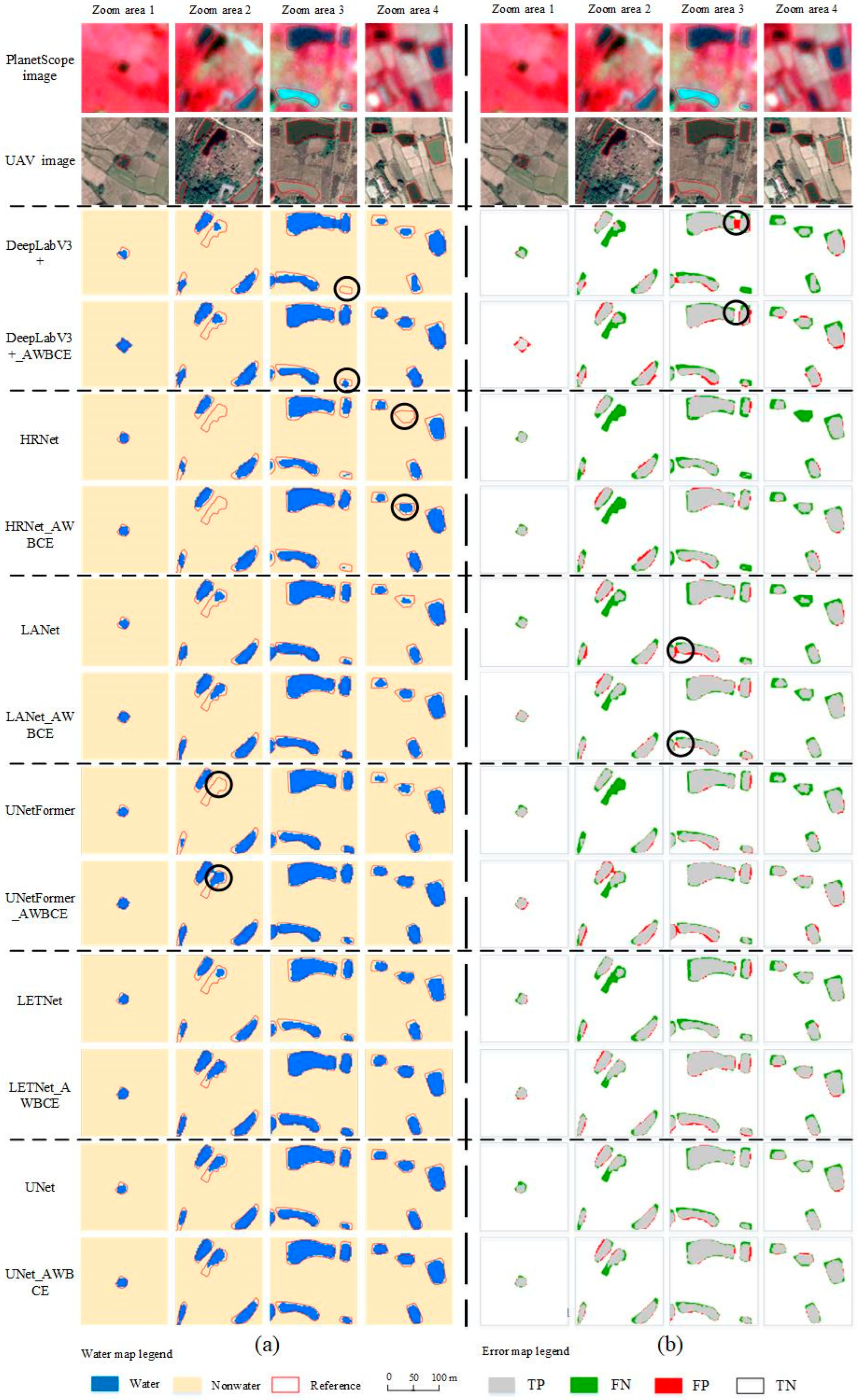
5.2.1. Results of Different Deep-Learning Models with and Without the Proposed AWBCE Loss in the Large Area Experiment

The surface water map generated from different models in a large area was compared in this study. Figure 10 demonstrates the difference between various models for some typical SWBs in the zoom areas. In general, in the predicted surface water maps, the models using BCE loss without using AWBCE loss predicted SWBs that were relatively smaller than the reference, whereas the models using AWBCE loss mapped larger sizes for these SWBs that better matched the shape of the SWBs in all zoom areas in the water maps. DeepLab V3+, HRNet, and UNetFormer failed to detect some SWBs, such as those highlighted in black circles in zoom areas 2, 3, and 4 in Figure 10; and DeepLab V3+_AWBCE, HRNet_AWBCE, and UNetFormer_AWBCE mapped parts of these SWBs. In general, UNet_AWBCE better mapped the boundary shape of SWBs than other models. In the error maps, the models using the BCE loss mapped more FN pixels (water incorrectly predicted as non-water highlighted in green color) than those using AWBCE loss for most models. In addition, DeepLabV3+ and LANet generated more FP pixels (non-water incorrectly predicted as water highlighted in red color) than DeepLabV3+_AWBCE and LANet_AWBCE in regions where the SWBs were adjacent to each other, highlighted with black circles in the zoom area 3. Among all the models, UNet_AWBCE generated the least FN and FP pixels in the green and red colors in the error maps, showing its advantage over the other models.

The overall accuracies of different deep-learning models were higher than 95% in

Table 4. The accuracy of the different models in the large area experiment. The highest accuracy values are highlighted in bold.

Models	OA (%)	UA (%)	PA (%)	F1	IoU	MCC
DeepLabV3+	95.9	98.9	92.8	0.958	0.919	0.920
DeepLabV3+_AWBCE	96.0	98.4	93.6	0.959	0.921	0.921
HRNet	95.9	99.2	92.6	0.958	0.919	0.921
HRNet_AWBCE	96.4	98.9	93.8	0.963	0.928	0.929
LANet	97.0	98.7	95.2	0.969	0.941	0.940
LANet_AWBCE	97.1	98.7	95.5	0.971	0.943	0.943
UNetFormer	96.0	99.0	92.9	0.959	0.921	0.922
UNetFormer_AWBCE	97.4	98.7	96.1	0.974	0.950	0.949
LETNet	96.4	99.1	93.7	0.963	0.929	0.930
LETNet_AWBCE	97.0	98.0	96.0	0.970	0.942	0.941
UNet	96.1	98.8	93.2	0.929	0.922	0.923
UNet_AWBCE	97.6	99.0	96.2	0.976	0.953	0.953

. All the models using the proposed AWBCE loss increased PA values, showing the advantage of the proposed AWBCE loss in reducing the omission errors for water pixels. It was noticed that reducing omission error usually indicates generating fewer FN pixels in green color in the error maps in Figure 10b. In addition, all the models using the proposed AWBCE loss enhanced OA, PA, F1, IoU, and MCC, respectively, highlighting its generalizability across different deep-learning architectures. Among these, UNet_AWBCE generated the highest OA, PA, F1, IoU, and MCC among models, a result similar to the result in the small area experiment.

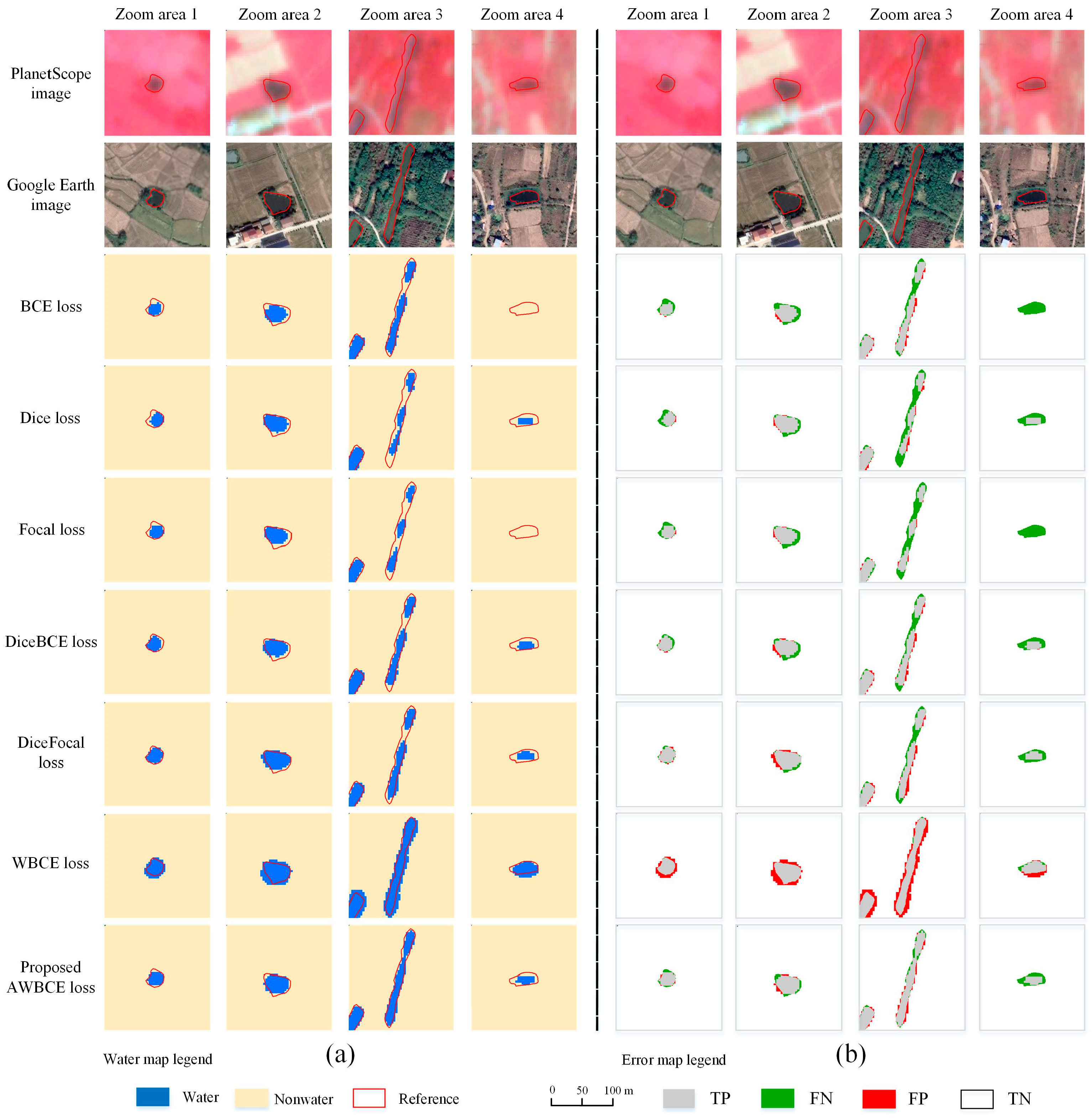
5.2.2. Comparison of Different Loss Functions for Addressing the Class Imbalance Problem in the Large Area Experiment

The models with different loss functions using UNet as the base model were compared, and the resulting water maps and error maps are shown in Figure 11. In general, the model using WBCE loss overestimated the number of water pixels, generated SWBs with enlarged shapes in the water maps and with more FP pixels (non-water incorrectly predicted as water) in red in the error maps, and generated the lowest UA values for water in

Table 5. The accuracies of the different loss functions using UNet as the base model in the large area experiment. The highest accuracy values are highlighted in bold.

Models	OA (%)	UA (%)	PA (%)	F1	IoU	MCC
BCE loss	96.1	98.8	93.2	0.929	0.922	0.923
Dice loss	96.7	99.5	94.0	0.966	0.935	0.936
Focal loss	96.4	99.6	93.2	0.963	0.928	0.930
DiceBCE loss	96.3	99.4	93.3	0.962	0.927	0.928
DiceFocal loss	97.2	99.2	95.2	0.972	0.945	0.945
WBCE loss	97.1	97.3	96.8	0.971	0.943	0.941
Proposed AWBCE loss	97.6	99.0	96.2	0.976	0.953	0.953

. The models using BCE loss and Focal loss failed to map the SWB in zoom area 4 in the water maps, and, thus, they generated more FN pixels (water incorrectly predicted as non-water) highlighted in green in the error map in Figure 11 and showed the lowest PA values for water in Table 5. In zoom area 3, only the models using WBCE and AWBCE loss predicted the ditch with continuous shapes, while the model with AWBCE loss better predicted the shape boundaries. In the quantitative metric in Table 5, the model with BCE loss which did not consider the class imbalance problem yielded the lowest OA, F1, IoU, and MCC values. In addition, the model with AWBCE loss had the highest OA, F1, IoU, and MCC values, showing the advantage of balancing both inter- and intra-class distributions in mapping SWBs.

6. Discussion

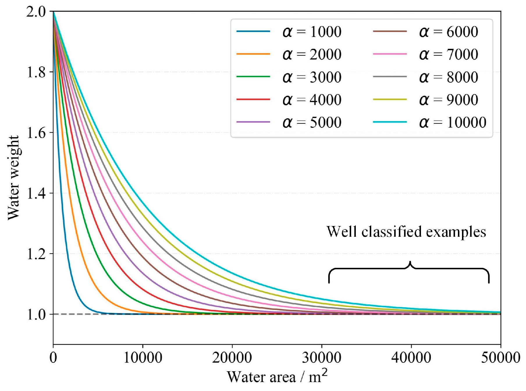
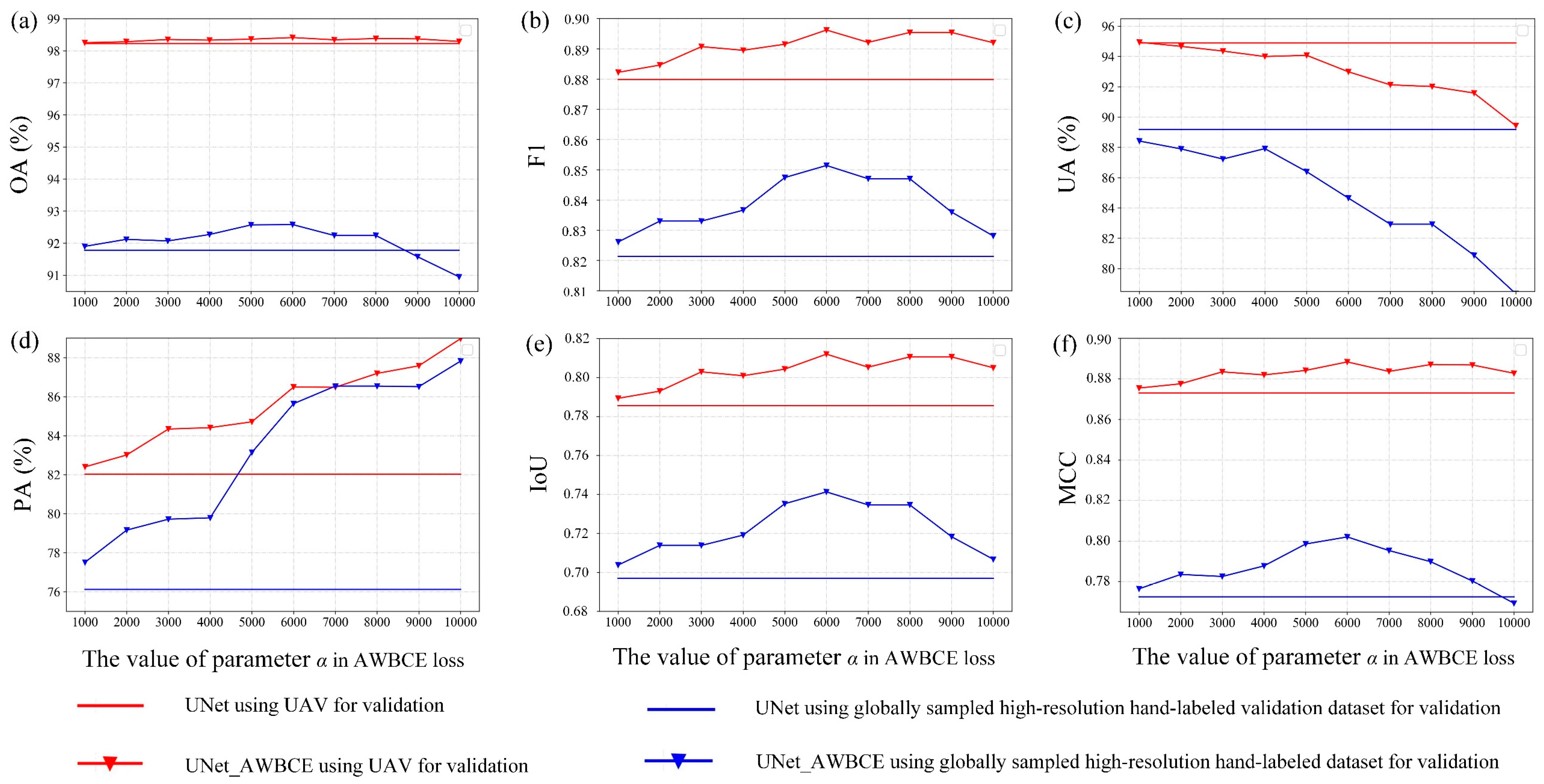
6.1. The Impact of Model Parameters

The impact of model parameters was analyzed in this section. The performance of the proposed AWBCE loss is mainly dependent on parameter $\alpha$ in Equation (6). The effect of parameter $\alpha$ of the AWBCE loss is examined using the UNet model (UNet_AWBCE) and compared with the standard BCE loss implemented in the UNet model (UNet). This comparison is made because these models achieved the highest OA, F1 score, IoU, and MCC values among those utilizing and not utilizing the AWBCE loss.

The accuracies were validated in the small area experiment using UAV data for validation because the reference data were delineated with a high spatial resolution of 2.5 cm. Additionally, the globally sampled high-resolution hand-labeled validation dataset for evaluating surface water extent maps, which is manually digitized from PlanetScope, is also used for validation [74]. This global dataset consists of 100 PlanetScope images, each with a size of 1024 × 1024 pixels. This dataset covers all 14 biomes and highlights urban and rural regions, lakes, and rivers, including braided rivers and coastal regions worldwide. The spatial distributions of the global sample points are in [74].

In Figure 12, in general, the values of OA, F1, IoU, and MCC from UNet_AWBCE increased as $\alpha$ increased when $\alpha$ was smaller than 6000, but decreased when $\alpha$ was larger than 6000 in both datasets. UNet_AWBCE generated OA, F1, PA, IoU, and MCC that were higher than those of UNet at different $\alpha$ values but generated UA that was lower than UNet in both datasets. The curves of UA decreased, and PA increased with the increase in $\alpha$. This is because the water weight increased with the increase in $\alpha$; thus, more water pixels were detected, which may lead to a decrease in omission error but an increase in commission error for water. The accuracy in the experiment using UAV for validation was higher than that using the globally sampled high-resolution hand-labeled validation dataset for validation, which is due to the fact that the training dataset and the validation data using UAV were from the nearby regions.

6.2. Reliability and Stability Analysis of the Models

The reliability and stability of the UNet_AWBCE model (which performed best in the aforementioned experiments) in mapping SWBs across various seasons were assessed. In this experiment, the 14,509 image patches were divided into five folds for cross-validation. Each time, four folds were used to train and validate the model, while the remaining fold was used for testing, and the process was repeated five times until every fold was used for testing. The training and validation datasets, each time, were further divided into 80% for model construction and 20% for validation. The acquisition dates of the 14,509 patches ranged mainly from July 2017 to November 2018, and are listed in

Table 6. The acquisition date of the PlanetScope imagery in the five folds cross-validation experiment.

Date	Date	Date	Date
26 May 2017	8 April 2018	25 August 2019	30 November 2020
17 July 2017	7 June 2018	4 March 2020	6 May 2021
23 July 2017	28 June 2018	20 March 2020	7 May 2021
2 January 2018	8 September 2018	26 April 2020	16 June 2021
12 January 2018	4 October 2018	20 May 2020	30 July 2021
28 March 2018	14 March 2019	10 October 2020	26 September 2021
1 April 2018	6 April 2019	24 October 2020	17 November 2021
7 April 2018	24 August 2019	10 November 2020	29 November 2021

. Given that the patches span various seasons and cover the majority of months, it is reasonable to consider them suitable for demonstrating the stability of the proposed method.

The accuracy of each fold is presented in

Table 7. The accuracies of the UNet_AWBCE model in the five-fold cross-validation experiment. The Ave. and St. dev. indicate average value and standard deviations.

Accuracy	Fold1	Fold2	Fold3	Fold4	Fold5	Ave.	St. dev.
OA (%)	99.2	99.1	99.1	99.1	99.2	99.1	0.049
UA (%)	94.2	94.7	94.0	94.3	95.1	94.5	0.393
PA (%)	93.3	93.0	93.2	93.2	93.1	93.2	0.102
F1	0.938	0.938	0.936	0.937	0.941	0.938	0.002
IoU	0.883	0.883	0.879	0.882	0.888	0.883	0.003
MCC	0.933	0.933	0.931	0.933	0.936	0.933	0.002

. The proposed UNet_AWBCE achieved an OA of 99.1% ± 0.049, an F1-score of 0.938 ± 0.002, an IoU of 0.883 ± 0.003, and an MCC of 0.933 ± 0.002. Furthermore, the table shows that the OA, UA, PA, F1, IoU, and MCC values across the five folds exhibit minimal variation. The notably small standard deviations further demonstrate the reliability and stability of the UNet_AWBCE model. The consistent and high performance of the model across multiple metrics underscores its capability for processing SWBs from different seasons.

6.3. Migration Experiments

To evaluate the effectiveness of the proposed AWBCE loss across different study areas, a migration experiment was conducted using three additional sites that were not included in previous experiments. The detailed characteristics of these sites are provided in

Table 8. Detailed information about the small scene images.

Site	Location	Image Size	Resolution	Data Source
1	30°53′~30°58′N, 113°6′~111°11′E	2578 × 3223	3 m	PlanetScope
2	30°19′~30°25′N, 113°23′~113°29′E	3335 × 3334	3 m	PlanetScope
3	31°15′~31°17′N, 112°35′~112°38′E	1667 × 1667	3 m	PlanetScope

: Site 1 represents a mountainous region, Site 2 represents an urbanized area, and Site 3 represents an agricultural zone, all containing SWBs such as fishponds and ditches. The UNet models with different loss functions, which were trained in the previous experiments, were tested for comparison.

As shown in

Table 9. The accuracies of the different loss functions using UNet as the base model in migration experiment. The highest accuracy values are highlighted in bold.

Models	OA (%)	UA (%)	PA (%)	F1	IoU	MCC
BCE loss	98.2	94.5	77.0	0.848	0.737	0.844
Dice loss	98.2	93.6	78.0	0.851	0.741	0.846
Focal loss	98.3	93.2	79.4	0.857	0.750	0.851
DiceBCE loss	98.2	91.4	79.7	0.851	0.741	0.844
DiceFocal loss	98.2	94.1	77.0	0.847	0.735	0.842
WBCE loss	97.8	78.9	91.4	0.847	0.734	0.838
Proposed AWBCE loss	98.5	93.5	82.8	0.878	0.783	0.872

, the UNet model with WBCE loss achieved the highest producer accuracy (PA) but the lowest user accuracy (UA), indicating a tendency to overestimate water pixels and produce enlarged SWB shapes in water maps—consistent with the findings in Table 3 and Table 5. In contrast, the UNet model with proposed AWBCE loss achieved the highest OA, F1-score, IoU, and MCC across different sites, demonstrating the superior performance of the proposed AWBCE loss for water mapping tasks.

6.4. Limitations and Future Works

Although deep-learning models have correctly mapped the shapes of the SWBs, challenges still exist. First, although the models with the proposed AWBCE generated the highest OA, F1, IoU, and MCC compared to those using other loss functions in most cases, they did not generate the highest PA and UA. In general, the models with Focal loss generated the highest UA but the lowest PA, while the models with WBCE loss generated the highest PA but the lowest UA, according to Table 2 and Table 4. This is because there is often a tradeoff between PA and UA.

Compared to the models with BCE loss without considering class imbalance, the model with the proposed AWBCE increased PA. The reason is that more attention was given to SWBs. Consequently, compared to the models using BCE loss without considering class imbalance, the models with the proposed AWBCE generated more water pixels and mapped the SWBs relatively larger sizes. Although PA has been increased, the proposed method may incorrectly predict non-water (i.e., the majority class) as water (i.e., the minority class), thereby decreasing UA as shown in Table 3. Since it is difficult to generate optimal results with both high PA and UA from a single model, future studies can focus on either combining different loss functions, or combining SWB segmentation results from different loss functions.

Second, the omission and commission errors are mostly found at the water–non-water boundaries, as shown in Figure 13. Although the water–non-water boundary is distinct in the Google Earth image, it is still blurred in the 3 m resolution PlanetScope image. Both UNet and UNet_AWBCE are likely to misclassify pixels at the border of the SWB where the PlanetScope imagery is blurred. It is difficult to visually distinguish the label of the sample points, highlighted in yellow in Figure 13. Future research should focus on the fusion of Google Earth imagery or other higher-resolution imagery with PlanetScope to delineate the boundary of SWBs more accurately. Additionally, we have used a random rotation function for data augmentation, and more data augmentation operations, such as random cropping, Gaussian blurring, and photometric distortions, could be explored to improve the generalization ability of the models.

7. Conclusions

In this study, an AWBCE loss was proposed to map SWBs while alleviating the class imbalance problem in relatively low latitudes. The proposed AWBCE loss not only assigned higher weights for water pixels to alleviate the inter-class imbalance problem between water and non-water, but also assigned higher weights for small water bodies than for large lakes to deal with the intra-class imbalance problem. In the experiments using UAV and WorldView-2 imagery from Google Earth for validation, the model with the proposed AWBCE loss increased the IoU, compared with different State-of-the-Art loss functions that address the class imbalance problem. The visual comparison shows that the proposed AWBCE loss better mapped the boundary shape of SWBs.

Among all the accuracy metrics, IoU and IoU_pSWB measure the model’s capability in detecting SWBs. Deep-learning methods with the proposed AWBCE demonstrated improved performance, increasing IoU by approximately 0.02 and IoU_pSWB by 0.03, highlighting its advantage in accurately delineating SWBs. Through the combination of various deep-learning methods (including DeepLabV3+, HRNet, LANet, UNetFormer, LETNet, and UNet) with different loss functions (including BCE loss, Dice loss, Focal loss, DiceBCE loss, DiceFocal loss, the WBCE loss, and the proposed AWBCE loss), we found that UNet with the proposed AWBCE loss achieved the highest accuracies in mapping SWBs. The results highlighted the need to address both inter- and intra-class imbalance problems in SWB mapping, and this paper demonstrates the effectiveness of solving this problem from the perspective of the loss function. The current study is critical for mapping SWBs with the popular, very high resolution PlanetScope daily imagery to improve the understanding of the dynamics of SWBs.

References

1. Holgerson, M.A.; Raymond, P.A. Large contribution to inland water CO2 and CH4 emissions from very small ponds. Nat. Geosci. 2016, 9, 222–226. [Google Scholar] [CrossRef]
2. Avis, C.A.; Weaver, A.J.; Meissner, K.J. Reduction in areal extent of high-latitude wetlands in response to permafrost thaw. Nat. Geosci. 2011, 4, 444–448. [Google Scholar] [CrossRef]
3. Mullen, A.L.; Watts, J.D.; Rogers, B.M.; Carroll, M.L.; Elder, C.D.; Noomah, J.; Williams, Z.; Caraballo-Vega, J.A.; Bredder, A.; Rickenbaugh, E.; et al. Using High-Resolution Satellite Imagery and Deep Learning to Track Dynamic Seasonality in Small Water Bodies. Geophys. Res. Lett. 2023, 50, e2022GL102327. [Google Scholar] [CrossRef]
4. Polishchuk, Y.M.; Bogdanov, A.N.; Muratov, I.N.; Polishchuk, V.Y.; Lim, A.; Manasypov, R.M.; Shirokova, L.S.; Pokrovsky, O.S. Minor contribution of small thaw ponds to the pools of carbon and methane in the inland waters of the permafrost-affected part of the Western Siberian Lowland. Environ. Res. Lett. 2018, 13, 1–16. [Google Scholar] [CrossRef]
5. Lv, M.; Wu, S.; Ma, M.; Huang, P.; Wen, Z.; Chen, J. Small water bodies in China: Spatial distribution and influencing factors. Sci. China Earth Sci. 2022, 65, 1431–1448. [Google Scholar] [CrossRef]
6. Perin, V.; Tulbure, M.G.; Gaines, M.D.; Reba, M.L.; Yaeger, M.A. A multi-sensor satellite imagery approach to monitor on-farm reservoirs. Remote Sens. Environ. 2021, 270, 112796. [Google Scholar] [CrossRef]
7. Chao Rodríguez, Y.; el Anjoumi, A.; Domínguez Gómez, J.A.; Rodríguez Pérez, D.; Rico, E. Using Landsat image time series to study a small water body in Northern Spain. Environ. Monit. Assess. 2014, 186, 3511–3522. [Google Scholar] [CrossRef]
8. Du, Y.; Zhang, Y.; Ling, F.; Wang, Q.; Li, W.; Li, X. Water Bodies’ Mapping from Sentinel-2 Imagery with Modified Normalized Difference Water Index at 10-m Spatial Resolution Produced by Sharpening the SWIR Band. Remote Sens. 2016, 8, 354. [Google Scholar] [CrossRef]
9. Li, Y.; Dang, B.; Zhang, Y.; Du, Z. Water body classification from high-resolution optical remote sensing imagery: Achievements and perspectives. ISPRS J. Photogramm. Remote Sens. 2022, 187, 306–327. [Google Scholar] [CrossRef]
10. Li, X.; Jia, X.; Yin, Z.; Du, Y.; Ling, F. Integrating MODIS and Landsat imagery to monitor the small water area variations of reservoirs. Sci. Remote Sens. 2022, 5, 100045. [Google Scholar] [CrossRef]
11. Ogilvie, A.; Belaud, G.; Massuel, S.; Mulligan, M.; Le Goulven, P.; Malaterre, P.-O.; Calvez, R. Combining Landsat observations with hydrological modelling for improved surface water monitoring of small lakes. J. Hydrol. 2018, 566, 109–121. [Google Scholar] [CrossRef]
12. Chen, Y.; Tang, L.; Kan, Z.; Bilal, M.; Li, Q. A novel water body extraction neural network (WBE-NN) for optical high-resolution multispectral imagery. J. Hydrol. 2020, 588, 125092. [Google Scholar] [CrossRef]
13. Pi, X.; Luo, Q.; Feng, L.; Xu, Y.; Tang, J.; Liang, X.; Ma, E.; Cheng, R.; Fensholt, R.; Brandt, M.; et al. Mapping global lake dynamics reveals the emerging roles of small lakes. Nat. Commun. 2022, 13, 5777. [Google Scholar] [CrossRef]
14. Ogilvie, A.; Belaud, G.; Massuel, S.; Mulligan, M.; Le Goulven, P.; Calvez, R. Surface water monitoring in small water bodies: Potential and limits of multi-sensor Landsat time series. Hydrol. Earth Syst. Sci. 2018, 22, 4349–4380. [Google Scholar] [CrossRef]
15. Dong, Y.; Fan, L.; Zhao, J.; Huang, S.; Geiß, C.; Wang, L.; Taubenböck, H. Mapping of small water bodies with integrated spatial information for time series images of optical remote sensing. J. Hydrol. 2022, 614, 128580. [Google Scholar] [CrossRef]
16. Crawford, C.J.; Roy, D.P.; Arab, S.; Barnes, C.; Vermote, E.; Hulley, G.; Gerace, A.; Choate, M.; Engebretson, C.; Micijevic, E.; et al. The 50-year Landsat collection 2 archive. Sci. Remote Sens. 2023, 8, 100103. [Google Scholar] [CrossRef]
17. Bie, W.; Fei, T.; Liu, X.; Liu, H.; Wu, G. Small water bodies mapped from Sentinel-2 MSI (MultiSpectral Imager) imagery with higher accuracy. Int. J. Remote Sens. 2020, 41, 7912–7930. [Google Scholar] [CrossRef]
18. Yan, L.; Roy, D.P.; Promkhambut, A.; Fox, J.; Zhai, Y. Automated extraction of aquaculture ponds from Sentinel-2 seasonal imagery—A validated case study in central Thailand. Sci. Remote Sens. 2022, 6, 100063. [Google Scholar] [CrossRef]
19. Freitas, P.; Vieira, G.; Canário, J.; Folhas, D.; Vincent, W.F. Identification of a Threshold Minimum Area for Reflectance Retrieval from Thermokarst Lakes and Ponds Using Full-Pixel Data from Sentinel-2. Remote Sens. 2019, 11, 657. [Google Scholar] [CrossRef]
20. Ji, Z.; Zhu, Y.; Pan, Y.; Zhu, X.; Zheng, X. Large-Scale Extraction and Mapping of Small Surface Water Bodies Based on Very High-Spatial-Resolution Satellite Images: A Case Study in Beijing, China. Water 2022, 14, 2889. [Google Scholar] [CrossRef]
21. Zhou, P.; Li, X.; Foody, G.M.; Boyd, D.S.; Wang, X.; Ling, F.; Zhang, Y.; Wang, Y.; Du, Y. Deep Feature and Domain Knowledge Fusion Network for Mapping Surface Water Bodies by Fusing Google Earth RGB and Sentinel-2 Images. IEEE Geosci. Remote Sens. Lett. 2023, 20, 1–5. [Google Scholar] [CrossRef]
22. Marta, S. Planet Imagery Product Specifications; Planet Labs: San Francisco, CA, USA; Volume 91, Available online: https://assets.planet.com/docs/Combined-Imagery-Product-Spec-Dec-2018.pdf (accessed on 15 August 2020).
23. Perin, V.; Roy, S.; Kington, J.; Harris, T.; Tulbure, M.G.; Stone, N.; Barsballe, T.; Reba, M.; Yaeger, M.A. Monitoring Small Water Bodies Using High Spatial and Temporal Resolution Analysis Ready Datasets. Remote Sens. 2021, 13, 5176. [Google Scholar] [CrossRef]
24. Buda, M.; Maki, A.; Mazurowski, M.A. A systematic study of the class imbalance problem in convolutional neural networks. Neural Netw. 2018, 106, 249–259. [Google Scholar] [CrossRef] [PubMed]
25. Chen, Z.; Duan, J.; Kang, L.; Qiu, G. Class-Imbalanced Deep Learning via a Class-Balanced Ensemble. IEEE Trans. Neural Netw. Learn. Syst. 2021, 33, 5626–5640. [Google Scholar] [CrossRef]
26. Galar, M.; Fernandez, A.; Barrenechea, E.; Bustince, H.; Herrera, F. A Review on Ensembles for the Class Imbalance Problem: Bagging-, Boosting-, and Hybrid-Based Approaches. IEEE Trans. Syst. Man Cybern. Part C Appl. Rev. 2012, 42, 463–484. [Google Scholar] [CrossRef]
27. Qayyum, N.; Ghuffar, S.; Ahmad, H.M.; Yousaf, A.; Shahid, I. Glacial Lakes Mapping Using Multi Satellite PlanetScope Imagery and Deep Learning. ISPRS Int. J. Geo Inf. 2020, 9, 560. [Google Scholar] [CrossRef]
28. He, H.; Garcia, E.A. Learning from Imbalanced Data. IEEE Trans. Knowl. Data Eng. 2009, 21, 1263–1284. [Google Scholar]
29. Li, K.; Wang, J.; Yao, J. Effectiveness of machine learning methods for water segmentation with ROI as the label: A case study of the Tuul River in Mongolia. Int. J. Appl. Earth Obs. Geoinf. 2021, 103, 102497. [Google Scholar] [CrossRef]
30. Sáez, J.A.; Krawczyk, B.; Woźniak, M. Analyzing the oversampling of different classes and types of examples in multi-class imbalanced datasets. Pattern Recognit. 2016, 57, 164–178. [Google Scholar] [CrossRef]
31. Chawla, N.V.; Bowyer, K.W.; Hall, L.O.; Kegelmeyer, W.P. SMOTE: Synthetic minority over-sampling technique. J. Artif. Intell. Res. 2002, 16, 321–357. [Google Scholar] [CrossRef]
32. Wang, S.; Liu, W.; Wu, J.; Cao, L.; Meng, Q.; Kennedy, P.J. Training deep neural networks on imbalanced data sets. In Proceedings of the 2016 International Joint Conference on Neural Networks (IJCNN), Vancouver, CA, Canada, 24–29 July 2016; pp. 4368–4374. [Google Scholar]
33. Han, H.; Wang, W.-Y.; Mao, B.-H. Borderline-SMOTE: A New Over-Sampling Method in Imbalanced Data Sets Learning. In Advances in Intelligent Computing; Springer: Berlin, Germany, 2005; pp. 878–887. [Google Scholar]
34. Mullick, S.S.; Datta, S.; Das, S. Generative adversarial minority oversampling. In Proceedings of the 2015 IEEE International Conference on Computer Vision (ICCV), Seoul, Republic of Korea, 27 October–2 November 2019; pp. 1695–1704. [Google Scholar]
35. Mariani, G.; Scheidegger, F.; Istrate, R.; Bekas, C.; Malossi, C. BAGAN: Data augmentation with balancing GAN. arXiv 2018, arXiv:1803.09655. [Google Scholar]
36. Dieste, Á.G.; Argüello, F.; Heras, D.B. ResBaGAN: A Residual Balancing GAN with Data Augmentation for Forest Mapping. IEEE J. Sel. Top. Appl. Earth Obs. Remote Sens. 2023, 16, 6428–6447. [Google Scholar] [CrossRef]
37. Wang, Q.; Lohse, J.P.; Doulgeris, A.P.; Eltoft, T. Data Augmentation for SAR Sea Ice and Water Classification Based on Per-Class Backscatter Variation with Incidence Angle. IEEE Trans. Geosci. Remote Sens. 2023, 61, 1–15. [Google Scholar] [CrossRef]
38. Jadon, S. A survey of loss functions for semantic segmentation. In Proceedings of the 2020 IEEE Conference on Computational Intelligence in Bioinformatics and Computational Biology (CIBCB), Via del Mar, FL, USA, 27–29 October 2020; pp. 1–7. [Google Scholar]
39. Song, Y.; Rui, X.; Li, J. AEDNet: An Attention-Based Encoder–Decoder Network for Urban Water Extraction From High Spatial Resolution Remote Sensing Images. IEEE J. Sel. Top. Appl. Earth Obs. Remote Sens. 2024, 17, 1286–1298. [Google Scholar] [CrossRef]
40. Galar, M.; Fernández, A.; Barrenechea, E.; Herrera, F. EUSBoost: Enhancing ensembles for highly imbalanced data-sets by evolutionary undersampling. Pattern Recognit. 2013, 46, 3460–3471. [Google Scholar] [CrossRef]
41. Lin, T.-Y.; Goyal, P.; Girshick, R.; He, K.; Dollar, P. Focal Loss for Dense Object Detection. In Proceedings of the IEEE International Conference on Computer Vision, Venice, FL, USA, 22–29 October 2017; pp. 2980–2988. [Google Scholar]
42. Xu, G.; Cao, H.; Dong, Y.; Yue, C.; Li, K.; Tong, Y. Focal Loss Function based DeepLabv3+ for Pathological Lymph Node Segmentation on PET/CT. In Proceedings of the 2020 2nd International Conference on Intelligent Medicine and Image Processing, Tianjin, China, 18 June 2020; pp. 24–28. [Google Scholar]
43. Bai, Y.; Wu, W.; Yang, Z.; Yu, J.; Zhao, B.; Liu, X.; Yang, H.; Mas, E.; Koshimura, S. Enhancement of Detecting Permanent Water and Temporary Water in Flood Disasters by Fusing Sentinel-1 and Sentinel-2 Imagery Using Deep Learning Algorithms: Demonstration of Sen1Floods11 Benchmark Datasets. Remote Sens. 2021, 13, 2220. [Google Scholar] [CrossRef]
44. Du, J.; Zhou, Y.; Liu, P.; Vong, C.M.; Wang, T. Parameter-Free Loss for Class-Imbalanced Deep Learning in Image Classification. IEEE Trans. Neural Netw. Learn. Syst. 2023, 34, 3234–3240. [Google Scholar] [CrossRef]
45. Hossain, M.S.; Betts, J.M.; Paplinski, A.P. Dual Focal Loss to address class imbalance in semantic segmentation. Neurocomputing 2021, 462, 69–87. [Google Scholar] [CrossRef]
46. Milletari, F.; Navab, N.; Ahmadi, S.A. V-Net: Fully Convolutional Neural Networks for Volumetric Medical Image Segmentation. In Proceedings of the 2016 Fourth International Conference on 3D Vision (3DV), Stanford, CA, USA, 25–28 October 2016; pp. 565–571. [Google Scholar]
47. Lima, R.P.d.; Karimzadeh, M. Model Ensemble With Dropout for Uncertainty Estimation in Sea Ice Segmentation Using Sentinel-1 SAR. IEEE Trans. Geosci. Remote Sens. 2023, 61, 1–15. [Google Scholar] [CrossRef]
48. Zhong, H.F.; Sun, Q.; Sun, H.M.; Jia, R.S. NT-Net: A Semantic Segmentation Network for Extracting Lake Water Bodies From Optical Remote Sensing Images Based on Transformer. IEEE Trans. Geosci. Remote Sens. 2022, 60, 1–13. [Google Scholar] [CrossRef]
49. Taghanaki, S.A.; Zheng, Y.; Kevin Zhou, S.; Georgescu, B.; Sharma, P.; Xu, D.; Comaniciu, D.; Hamarneh, G. Combo loss: Handling input and output imbalance in multi-organ segmentation. Comput. Med. Imaging Graph. 2019, 75, 24–33. [Google Scholar] [CrossRef] [PubMed]
50. Bai, H.; Cheng, J.; Su, Y.; Liu, S.; Liu, X. Calibrated Focal Loss for Semantic Labeling of High-Resolution Remote Sensing Images. IEEE J. Sel. Top. Appl. Earth Obs. Remote Sens. 2022, 15, 6531–6547. [Google Scholar] [CrossRef]
51. Zhou, Y.; Yang, K.; Ma, F.; Hu, W.; Zhang, F. Water–Land Segmentation via Structure-Aware CNN–Transformer Network on Large-Scale SAR Data. IEEE Sens. J. 2022, 23, 1408–1422. [Google Scholar] [CrossRef]
52. Li, Y.; Zhou, Y.; Zhang, Y.; Zhong, L.; Wang, J.; Chen, J. DKDFN: Domain Knowledge-Guided deep collaborative fusion network for multimodal unitemporal remote sensing land cover classification. ISPRS J. Photogramm. Remote Sens. 2022, 186, 170–189. [Google Scholar] [CrossRef]
53. Azad, R.; Heidary, M.; Yilmaz, K.; Hüttemann, M.; Karimijafarbigloo, S.; Wu, Y.; Schmeink, A.; Merhof, D. Loss Functions in the Era of Semantic Segmentation: A Survey and Outlook. arXiv 2023, arXiv:2312.05391. [Google Scholar]
54. Xu, J.; Zhao, Y.; Lyu, H.; Liu, H.; Dong, X.; Li, Y.; Cao, K.; Xu, J.; Li, Y.; Wang, H.; et al. A semianalytical algorithm for estimating particulate composition in inland waters based on Sentinel-3 OLCI images. J. Hydrol. 2022, 608, 127617. [Google Scholar] [CrossRef]
55. Kabir, S.M.I.; Ahmari, H. Evaluating the effect of sediment color on water radiance and suspended sediment concentration using digital imagery. J. Hydrol. 2020, 589, 125189. [Google Scholar] [CrossRef]
56. Dang, B.; Li, Y. MSResNet: Multiscale Residual Network via Self-Supervised Learning for Water-Body Detection in Remote Sensing Imagery. Remote Sens. 2021, 13, 3122. [Google Scholar] [CrossRef]
57. Tong, X.-Y.; Xia, G.-S.; Lu, Q.; Shen, H.; Li, S.; You, S.; Zhang, L. Land-cover classification with high-resolution remote sensing images using transferable deep models. Remote Sens. Environ. 2020, 237, 111322. [Google Scholar] [CrossRef]
58. Valman, S.J.; Boyd, D.S.; Carbonneau, P.E.; Johnson, M.F.; Dugdale, S.J. An AI approach to operationalise global daily PlanetScope satellite imagery for river water masking. Remote Sens. Environ. 2024, 301, 113932. [Google Scholar] [CrossRef]
59. Xiang, D.; Zhang, X.; Wu, W.; Liu, H. DensePPMUNet-a: A Robust Deep Learning Network for Segmenting Water Bodies From Aerial Images. IEEE Trans. Geosci. Remote Sens. 2023, 61, 1–11. [Google Scholar] [CrossRef]
60. Pihur, V.; Datta, S.; Datta, S. Weighted rank aggregation of cluster validation measures: A Monte Carlo cross-entropy approach. Bioinformatics 2007, 23, 1607–1615. [Google Scholar] [CrossRef] [PubMed]
61. Chen, L.-C.; Papandreou, G.; Schroff, F.; Adam, H. Rethinking Atrous Convolution for Semantic Image Segmentation. arXiv 2017, arXiv:1706.05587. [Google Scholar]
62. Sun, K.; Xiao, B.; Liu, D.; Wang, J. Deep high-resolution representation learning for human pose estimation. In Proceedings of the IEEE Conference on Computer Vision and Pattern Recognition (CVPR), Long Beach, CA, USA, 16–20 June 2019; pp. 5693–5703. [Google Scholar]
63. Ding, L.; Tang, H.; Bruzzone, L. LANet: Local Attention Embedding to Improve the Semantic Segmentation of Remote Sensing Images. IEEE Trans. Geosci. Remote Sens. 2021, 59, 426–435. [Google Scholar] [CrossRef]
64. Ronneberger, O.; Fischer, P.; Brox, T. U-Net: Convolutional Networks for Biomedical Image Segmentation. In Proceedings of the International Conference on Medical Image Computing and Computer-Assisted Intervention (MICCAI), Munich, Germany, 5–9 October 2015; pp. 234–241. [Google Scholar]
65. Wang, L.; Li, R.; Zhang, C.; Fang, S.; Duan, C.; Meng, X.; Atkinson, P.M. UNetFormer: A UNet-like transformer for efficient semantic segmentation of remote sensing urban scene imagery. ISPRS J. Photogramm. Remote Sens. 2022, 190, 196–214. [Google Scholar] [CrossRef]
66. Xu, G.; Li, J.; Gao, G.; Lu, H.; Yang, J.; Yue, D. Lightweight Real-Time Semantic Segmentation Network With Efficient Transformer and CNN. IEEE Trans. Intell. Transp. Syst. 2023, 24, 15897–15906. [Google Scholar] [CrossRef]
67. Yeung, M.; Sala, E.; Schönlieb, C.-B.; Rundo, L. Unified Focal loss: Generalising Dice and cross entropy-based losses to handle class imbalanced medical image segmentation. Comput. Med. Imaging Graph. 2022, 95, 102026. [Google Scholar] [CrossRef]
68. Gammoudi, I.; Ghozi, R.; Mahjoub, M.A. HDFU-Net: An Improved Version of U-Net using a Hybrid Dice Focal Loss Function for Multi-modal Brain Tumor Image Segmentation. In Proceedings of the 2022 International Conference on Cyberworlds (CW), Kanazawa, Japan, 27–29 September 2022; pp. 71–78. [Google Scholar]
69. Zhou, P.; Li, X.; Zhang, Y.; Wang, Y.; Li, Y.; Li, X.; Zhou, C.; Shen, L.; Du, Y. Attention is all you need. IEEE J. Sel. Top. Appl. Earth Obs. Remote Sens. 2024, 18, 2541–2562. [Google Scholar] [CrossRef]
70. LeCun, Y.; Bengio, Y.; Hinton, G. Deep learning. Nature 2015, 521, 436–444. [Google Scholar] [CrossRef]
71. Kingma, D.P.; Ba, J.L. Adam: A method for stochastic optimization. arXiv 2014, arXiv:1412.6980. [Google Scholar]
72. Maxwell, A.E.; Bester, M.S.; Ramezan, C.A. Enhancing Reproducibility and Replicability in Remote Sensing Deep Learning Research and Practice. Remote Sens. 2022, 14, 5760. [Google Scholar] [CrossRef]
73. Sharma, R.; Tsiamyrtzis, P.; Webb, A.G.; Seimenis, I.; Loukas, C.; Leiss, E.; Tsekos, N.V. A Deep Learning Approach to Upscaling “Low-Quality” MR Images: An In Silico Comparison Study Based on the UNet Framework. Appl. Sci. 2022, 12, 11758. [Google Scholar] [CrossRef]
74. Mukherjee, R.; Policelli, F.; Wang, R.; Arellano-Thompson, E.; Tellman, B.; Sharma, P.; Zhang, Z.; Giezendanner, J. A globally sampled high-resolution hand-labeled validation dataset for evaluating surface water extent maps. Earth Syst. Sci. Data 2024, 16, 4311–4323. [Google Scholar] [CrossRef]
Figure 1. The overview of the study area. (a) The location of the study area (highlighted with red boundary) and the locations of images in the PlanetScope-based SWB dataset. (b) Examples of 3 m PlanetScope false-color images of different water body types and the corresponding water label maps that were manually digitized and used for training the CNN. The dataset contains 14,509 patches of PlanetScope images (512 × 512 pixels) and the corresponding water labels.
Remotesensing 17 01868 g001
Figure 2. The process of estimating the weights for water pixels based on the area of each water body in the proposed AWBCE loss. (a) Water–non-water label map. (b) DN value in the water–non-water binary map. (c) Water labels indicate different water body objects. (d) The water area map in which different green colors indicate different areas for water bodies. (e) The curve shows the conversion from the water area to the weight of water pixels according to Equation (6). (f) The weighted map used for training.
Remotesensing 17 01868 g002
Figure 3. The curves showing the water weight of Wi with the change in water area with different α values in Equation (6).
Remotesensing 17 01868 g003
Figure 4. PlanetScope false-color image and the unmanned aerial vehicle (UAV) RGB image. (a) PlanetScope image. (b) UAV image.
Remotesensing 17 01868 g004
Figure 5. The false-color PlanetScope image of the study area and validation point in the study area. (a) PlanetScope imagery of the entire study area. (b) The distribution of validation points in black points. A total of 12,518 samples were used for validation.
Remotesensing 17 01868 g005
Figure 6. The visual comparison between deep-learning models with and without AWBCE loss. (a) PlanetScope false-color images, UAV images, and the water maps from different models with and without AWBCE loss. The reference water boundaries are presented with red lines in (a). (b) The corresponding error maps. The green pixels in the error map represented FN (water incorrectly predicted as non-water), the red pixels in the error map represented FP (non-water incorrectly predicted as water), the grey pixels in the error map represented TP (water correctly predicted as water), and the white pixels in the error map represented TN (non-water correctly predicted as non-water). Each zoom area has an area of 12,100 m2.
Remotesensing 17 01868 g006
Figure 7. IoUpSWB score of the size of SWBs assessed by the UAV image in different maps. (a) DeepLabV3+. (b) DeepLabV3+_AWBCE. (c) HRNet. (d) HRNet_AWBCE. (e) LANet. (f) LANet_AWBCE. (g) UNetFormer. (h) UNetFormer_AWBCE. (i) LETNet. (j) LETNet_AWBCE. (k) UNet. (l) UNet_AWBCE.
Remotesensing 17 01868 g007
Figure 8. The visual comparison of results using different loss functions. (a) PlanetScope false-color images, UAV images, and the water maps from UNet with different loss functions. The reference water boundaries are presented with red lines. (b) The corresponding error maps. The green pixels in the error map represented FN (water incorrectly predicted as non-water), the red pixels in the error map represented FP (non-water incorrectly predicted as water), the grey pixels in the error map represented TP (water correctly predicted as water), and the white pixels in the error map represented TN (non-water correctly predicted as non-water). Each zoom area has an area of 12,100 m2.
Remotesensing 17 01868 g008
Figure 9. IoUpSWB score of the size of SWBs from the UNet model with different loss functions assessed by the UAV image in different maps. (a) Model with BCE loss. (b) Model with Dice loss. (c) Model with Focal loss. (d) Model with DiceBCE loss. (e) Model with DiceFocal loss. (f) Model with WBCE loss. (g) Model with the proposed AWBCE loss.
Remotesensing 17 01868 g009
Figure 10. The visual comparison between different models with and without AWBCE loss in large area experiment. (a) PlanetScope false-color images, WorldView-2 RGB images from Google Earth, and the water maps from different models with and without AWBCE loss. The reference water boundaries are presented with red lines. (b) The corresponding error maps. The green pixels in the error map represented FN (water incorrectly predicted as non-water), the red pixels in the error map represented FP (non-water incorrectly predicted as water), the grey pixels in the error map represented TP (water correctly predicted as water), and the white pixels in the error map represented TN (non-water correctly predicted as non-water). Each zoom area has an area of 28,900 m2.
Remotesensing 17 01868 g010
Figure 11. Visual comparison of different loss functions in large area experiment. (a) PlanetScope false-color images, WorldView-2 RGB images from Google Earth, and the water maps from UNet with different loss functions. The reference water boundaries are presented with red lines. (b) The corresponding error maps. The green pixels in the error map represented FN (water incorrectly predicted as non-water), the red pixels in the error map represented FP (non-water incorrectly predicted as water), the grey pixels in the error map represented TP (water correctly predicted as water), and the white pixels in the error map represented TN (non-water correctly predicted as non-water). Each zoom area has an area of 28,900 m2.
Remotesensing 17 01868 g011
Figure 12. The accuracy of UNet_AWBCE with different values of the weight α and UNet with the standard BCE loss using UAV for validation and using a globally sampled high-resolution hand-labeled validation dataset for validation. (a) OA. (b) F1. (c) UA. (d) PA. (e) IoU. (f) MCC.
Remotesensing 17 01868 g012
Figure 13. The location of the validation samples mapped with omission and commission errors at the water–non-water boundaries for the deep-learning models predicted maps.
Remotesensing 17 01868 g013