Abstract
Direct Position Estimation (DPE) is an alternative GNSS positioning method that models received satellite signals as a function of the receiver’s navigation state, allowing for the direct estimation of position, velocity, and time within the navigation domain. However, existing DPE algorithms face significant challenges due to the non-convex nature of the optimization problem and the large solution space, resulting in high computational complexity. To address these challenges, this paper introduces a framework for searching for navigation solutions in DPE through swarm intelligence algorithms, combined with a low-complexity correlation approach. Furthermore, an adaptive Dung Beetle Optimization (ADBO) algorithm is developed. By leveraging insights from fitness landscape analysis, the ADBO algorithm dynamically adjusts subpopulation proportions and the convergence factor while incorporating hybrid mutation strategies for effective adaptation to various types of optimization problems. Benchmark function tests demonstrate that the ADBO algorithm achieves superior convergence performance compared with other popular swarm intelligence algorithms. Both extensive simulations and real GNSS data experiments further validate that the proposed framework, incorporating the ADBO algorithm, achieves improved positioning accuracy compared to traditional positioning methods while outperforming traditional search algorithms and other swarm intelligence algorithms in both accuracy and computational efficiency.
1. Introduction
Global Navigation Satellite Systems (GNSS) offer positioning services through a common method known as the two-step procedure (2SP): satellite signals are independently processed to derive synchronization parameters, which are subsequently used for receiver multilateration to estimate the receiver’s position, velocity, and time (PVT) state. While effective in open-sky environments, 2SP-based receivers encounter accuracy and stability challenges in complex scenarios, including jamming, multipath, and channel fading. These limitations stem from the inability of the 2SP to ensure that positioning parameters correspond to the same PVT state, thereby hindering its overall performance.
Recently, the growing demand for high-precision positioning and navigation services in challenging environments has highlighted the limitations of traditional positioning methods. With advancements in data transmission and computational capabilities, there has been increasing interest in Direct Position Estimation (DPE), also referred to as the one-step procedure, which involves obtaining the Maximum Likelihood estimate (MLE) of the PVT by directly solving the problem in the navigation domain, where signals from all visible satellites are processed jointly [1,2,3]. By eliminating intermediate estimation steps, DPE can partially mitigate some of the shortcomings of 2SP, such as degradation in position accuracy due to near–far resistance and severe channel fading conditions [4]. Despite its benefits, DPE presents a non-convex optimization problem, which makes it unsuitable for gradient-based algorithms and highly dependent on the optimization algorithm employed [5]. One such method, the Space Alternating Generalised Expectation-Maximization (SAGE) algorithm, decomposes a multi-dimensional search into a series of uni-dimensional searches [6]. However, as the clock dimension is not separable, an incorrect time estimate in the initial iteration can cause SAGE to converge to an incorrect result [7]. Another method uses the Accelerated Random Search (ARS) algorithm [8]. As a variant of the random search algorithm, its mechanism of adaptively adjusting the search radius enables dynamic coordination of the balance between global and local searches [9]. However, the performance of ARS highly depends on the setting of parameters, such as the initial search radius, contraction factor, and iterations. Currently, grid-based search algorithms remain the primary solution for DPE. Although assisted GPS (A-GPS) can provide a priori position–time information to effectively reduce the search space, the computational burden of performing signal correlation across a large number of candidate points remains a significant challenge.
To overcome these limitations, various approaches have sought to improve search efficiency. One of the most effective methods is the multi-resolution grid (MRG) method, which reduces the number of computational points by adjusting the grid size at each stage [10,11,12]. This method also uses an averaged correlogram at the search initiation to accelerate the process. However, generating the correlogram requires calculating the correlation value for each candidate point, which is computationally intensive. Another approach involves using a pseudorange correlogram-based algorithm to significantly reduce the correlation process computational load [13], although it does not account for the impact of the satellite elevation on correlation values. While these methods can accelerate the correlation process, they do not alleviate one of the most significant challenges of DPE: the need to evaluate a large number of candidates.
Swarm intelligence optimizers have been widely used to solve non-convex optimization problems in engineering fields, including positioning systems. An expanded and contracted Pigeon-Inspired Optimization (PIO) algorithm was developed for Collective Detection, a combined GNSS signal acquisition method [14]. In [15], an improved Particle Swarm Optimization (PSO) algorithm with an adaptive search space and elite reservation strategy was proposed for real-time estimation of the fractional part of the inter-system phase bias. Additionally, ref. [16] introduced a PSO–backpropagation neural network to model variations in GNSS broadcast ephemeris orbit errors. In recent years, numerous new SI algorithms have been widely adopted, including the Grey Wolf Optimization (GWO) algorithm [17], the Harris Hawks Optimization (HHO) algorithm [18], the Sparrow Search Algorithm (SSA) [19], and the Parrot Optimization (PO) algorithm [20]. Among these, the Dung Beetle Optimization (DBO) algorithm [21] is a novel optimization algorithm inspired by the ball-rolling, spawning, foraging, and stealing behaviors of dung beetles [22]. It stands out for its parallelized approach, offering faster convergence, enhanced accuracy, and robustness when dealing with complex scenarios [23,24,25]. While diverse behaviors endow DBO with flexibility, certain limitations remain. In particular, the fixed population ratios and search range settings restrict its ability to adaptively leverage these diverse behaviors in more challenging scenarios. Furthermore, like other swarm intelligence algorithms, the standard DBO still tends to get trapped in a local optimum when faced with high-dimensional, strongly nonlinear problems like DPE. To address these issues, we propose an adaptive DBO algorithm (ADBO) based on the concept of Fitness Landscape Analysis (FLA), which is connected to auto-tuning and the development of intelligent algorithms for complex systems [26,27]. This allows the ADBO algorithm to dynamically adjust its search strategy more effectively to varying optimization landscapes, with two key enhancements. The ADBO algorithm adjusts the proportion of foraging and spawning dung beetles and the convergence factor based on Fitness Distance Correlation (FDC). This approach adapts the balance between global and local search capabilities based on the landscape characteristics encountered by the population. Additionally, a hybrid mutation strategy combining Cauchy and Gaussian mutations is applied, with coefficients adjusted according to the ruggedness of the optimization problem. This approach enhances local exploration capabilities and reduces premature convergence risk.
The main contributions of this article are as follows. First, we propose a DPE-SI framework, which incorporates a low-complexity correlation approach and a swarm intelligence-based navigation solution search approach, effectively reducing the computational cost required for DPE. It is worth mentioning that this is the first attempt to apply swarm intelligence algorithms to DPE. Second, a novel ADBO algorithm is proposed, including a detailed explanation of its dynamic search strategy adjustments based on FLA. Benchmark function tests validate that the proposed ADBO algorithm outperforms other swarm intelligence algorithms. Next, the ADBO and other algorithms are applied to the proposed DPE-SI framework, with their performance compared against MRG, ARS, and 2SP methods in simulated signal experiments. Finally, the proposed framework is validated using real GNSS data in both static and dynamic receiver scenarios. Experimental results indicate that the DPE-SI framework with the ADBO algorithm provides higher positioning accuracy and improved stability with lower computational costs.
The rest of this paper is organized as follows. Section 2.1 describes the optimization model of DPE and proposes a DPE-SI framework for implementing DPE with a low-computation correlation approach. In Section 2.3.2, the proposed ADBO algorithm is presented and discussed in detail. Section 2.3.3 evaluates the convergence performance of ADBO against seven popular swarm intelligence algorithms using benchmark test functions. Section 3 provides the positioning results based on both simulated signals and real GNSS data. Finally, we conclude this paper in Section 5.
2. Materials and Methods
2.1. Optimization Problem of DPE
GNSS consists of a network of satellites orbiting the Earth, each transmitting predefined messages to the receivers on the ground. The signals captured by receivers are composed of a combination of structured plane waves, representing the line-of-sight (LOS) signals from visible satellites, distorted by thermal noise and possibly affected by external interference. Considering there are M visible satellites, the received complex baseband signal sampled at time can be expressed as
where and denote the signal amplitude and the known PRN codes of the i-th satellite, respectively. and denote the time delay and Doppler shift of the i-th satellite. denotes the noise, generally assumed to be zero-mean additive white Gaussian noise (AWGN).
If a receiver observes K snapshots, the signal model can be rearranged into matrix form as
where is the received signal vector, is the vector of complex signal amplitudes, is the AWGN vector, and is the local signal replica matrix, which is a function of parameter vectors and . Each component is defined by the delayed and Doppler-shifted signal envelope:
Conventional 2SP-based receivers handle each satellite signal independently, conducting a two-dimensional search to estimate parameters such as and . Based on a collection of K snapshots, the optimization problem can be expressed as
where stands for the Hermitian transpose operation and the operator denotes the -norm of a vector. After determining these parameters, the receiver calculates its position through trilateration. This widely used 2SP is favored for its computational simplicity and ease of implementation. However, when the signal channel deteriorates, significant errors may occur in the estimated carrier and code phase, leading to tracking loop loss of lock and rendering traditional GNSS receivers inoperative.
DPE leverages the relationship between the PVT state of a receiver and the time delay and Doppler shift of the received GNSS signal. Essentially, and can be expressed as functions of the PVT state :
where is the PVT state of the receiver, denotes the position of the receiver, and denotes the velocity of the receiver, and are the receiver clock bias and drift. Note that this is a simplified model. First, atmospheric-related errors, including ionospheric and tropospheric delays, are not explicitly modeled in the signal delay term . Instead, these effects are assumed to be mitigated through differential GNSS corrections or pre-calibrated error models. This is acceptable since our focus is on evaluating the robustness and efficiency of the proposed DPE algorithm, not detailed signal error modeling. Second, although GNSS systems provide carrier-phase observations, this study does not utilize phase-based positioning. The proposed method operates on complex baseband correlation outputs, where no carrier-phase ambiguity resolution is required. The polarity ambiguity introduced by modulation is resolved by detecting the telemetry preamble. Thereby, the time-frequency parameterization model of the received signals in (2) can be represented by the parameter vector in DPE:
The fundamental concept of DPE involves the simultaneous processing of observations from all visible satellites. Differing from traditional 2SP, it directly correlates PVT estimates with the received signal in the navigation domain. Note that the tilde symbol is used to denote the candidate’s parameters. By calculating and for each satellite, a signal replica for each candidate PVT is generated and correlated with the received signal. The correlation values of all candidate points are then combined into a correlogram, where the result with the highest correlation value yields the MLE of the PVT. The corresponding optimization problem is given by
DPE usually employs a global search strategy to determine the candidate corresponding to the maximum correlation value. By synthesizing information from all satellite signals simultaneously, DPE shows improved robustness compared with traditional methods, thus enabling the receiver to maintain high positioning stability in complex environments.
2.2. Low-Complexity Correlation Approach
In (6), the direct correlation calculation at the signal level is the cause of the high computational complexity of the DPE method. Theoretical studies have shown that although the direct correlation calculation can effectively suppress the cross-correlation interference, its effect on accuracy improvement is relatively limited in terms of the main source of localization errors [4]. In contrast, an alternative correlation calculation method can reduce the computational complexity while retaining the framework of the DPE and its joint processing in the navigation domain [13]. Specifically, using the autocorrelation function of the differences in time delay and Doppler shift between a candidate point and the satellite has been proposed to reduce complexity while ensuring that the correlation values correspond to the position domain, thus maintaining the dimensional consistency of DPE estimation. Moreover, it has been demonstrated that the correlation values for time delay and Doppler shift can be estimated independently with minimal accuracy loss [28]. By applying (4), the eight-dimensional optimization problem in (6) can be separated into two four-dimensional correlation functions for time delay and Doppler shift, respectively:
where and represent the deviations of the candidate’s time delay and Doppler shift from the true values for the i-th satellite. represents the chip period of the PRN code. Notably, in static or low-speed dynamic scenarios where the velocity and clock drift are considered fixed, the MLE of position and time bias can be derived from (7). By leveraging the relationship between the code phase of the GNSS signal and the candidate’s position and clock bias, the correlation function can be approximated by a pseudorange-based function to optimize the calculation:
Beyond ensuring dimensional consistency, DPE inherently incorporates the optimal weighting of different satellites in (6), which is crucial for maintaining the validity of the MLE criterion [29]. Consequently, when performing correlation approximation, it is necessary to reassign weights for individual satellites. Since the approximated correlation function is based on pseudoranges, factors influencing pseudorange measurements must be considered. By analyzing the variation of pseudorange errors with satellite elevation and carrier-to-noise ratio (), Tay and Marais [30] proposed a weighting model for LOS signal measurements, given by
where and represent the elevation and of the i-th satellite, respectively. To better replicate the implicit weights of the various satellites derived from the signal correlations received by the DPE, these weights are incorporated into (9). Consequently, the low-computation correlation approach accounting for both signal power and elevation is given by
In this approach, the correlation value of a candidate is directly calculated based on its time delay relative to the visible satellite. Additionally, the two factors that most affect the magnitude of the correlation value, the elevation and power of the signal, are taken into account to ensure the accuracy of the approximate correlation value. Instead of conducting intensive correlation calculations with signal replicas generated by the candidate’s PVT and the received signal, the correlation process is replaced by the autocorrelation function by comparing the time delay for each candidate with that of the received signal.
2.3. Adaptive DBO for DPE
2.3.1. DPE-SI Framework
Without loss of generality, we consider the feasible solution space provided a priori by A-GPS to be a Cartesian space with the same dimensions as the parameters of interest, denoted as . Therefore, by replacing the optimization function in (6) with (11), we formulate a position–time-related optimization problem as follows:
The process for solving the optimization problem in (12) within the large navigation domain directly affects the accuracy and computational cost, playing a crucial role in DPE implementation. Equation (11) shows that both satellite geometry and influence the objective function (12). This time-varying characteristic shifts the modality of the objective function, increasing the difficulty of solving the optimization problem. For clarity, we assume that the z coordinate and the clock bias are known, enabling two-dimensions visualization. Figure 1 shows the optimization function (12) evaluated with seven satellites under coordinate errors, and . These prevalent local optima in DPE limit the implementation of traditional optimization algorithms.
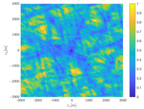
Figure 1.
Optimization problem in (12) as a function of the unknown two-dimensions receiver position and .
Swarm intelligence algorithms have gained popularity for their enhanced ability to effectively explore the solution space, making them well suited for addressing the optimization challenges in DPE. Based on these advantages, we propose the DPE-SI framework. In this framework, a population of L individuals is engaged to solve a four-dimensional problem related to position and time. The boundaries for each dimension are set by the feasible navigation space provided by A-GPS prior information. The fitness function in (12) evaluates the correlation between signal replicas and received signals, with each individual’s fitness value indicating the signal matching degree. The position and time states of individuals are iteratively updated to explore the search space and identify the optimal solution. The schematic flowchart of the DPE-SI framework is shown in Figure 2. The swarm intelligence algorithm governs the exploration and exploitation behavior of individuals within the search space, and its selection directly influences the positioning accuracy and computational efficiency of the framework.
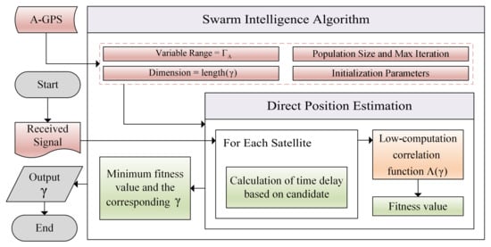
Figure 2.
Flowchart of the proposed DPE-SI framework.
2.3.2. Adaptive DBO Algorithm
In order to search for navigational solutions for DPEs more efficiently, high-performance optimization algorithms are essential. Therefore, we improve the algorithm for DBO to further enhance its search performance. In this section, the basic principle of DBO is first briefly introduced. Subsequently, an improved ADBO algorithm is proposed to enhance its adaptability and search capability in complex optimization problems.
The Standard DBO Algorithm
The DBO algorithm updates the population’s positions by simulating four natural behaviors of dung beetles: ball-rolling, spawning, foraging, and stealing. These behaviors correspond to four types of dung beetles: rolling, spawning, foraging, and stealing dung beetles, with the four dung beetles constituting a fixed proportion of the population of , , , and . Each type of dung beetle uses a distinct positional update strategy, working together to collaboratively search for the optimal solution.
Ball-rolling behavior: In nature, the dung beetles use the sun for navigation to maintain a straight path while rolling their dung balls. The position of the ball-rolling dung beetle is updated according to (13) when it encounters no obstacles
where t denotes the iteration number, represents the position of the dung beetle at iteration t. The coefficient a determines whether the dung beetle deviates from its original direction (1 indicates no deviation, indicates deviation). is the defect factor, originally set to , and is a constant, set to in the original code. denotes the global worst position. simulates solar illumination, with a larger indicating the dung beetle is further from the light source. If an obstacle is encountered, the dung beetle must reorient itself by dancing on the dung ball to find a new rolling route, updating its position as shown in (14):
where is the deflection angle, and when , it means that the position is not updated.
Reproductive behavior: Dung beetles roll their dung balls to a safe area for females to lay eggs and protect their offspring. The safe area is defined by
where denotes the current local optimal position, and and denote the lower and upper bounds of the optimization problem, respectively. and denote the lower and upper bounds of the spawning region, is the convergence factor, and is the maximum number of iterations.
Afterward, female dung beetles will each lay one egg per iteration within the brood balls in this safety area, updating the position as
If the position exceeds the safety area, it is adjusted as
where is the position of the l-th brood ball at the t-th iteration, and and are independent random vectors with the same dimension as the optimization problem.
Foraging behavior: The eggs will grow into dung beetles and come out from the ground to forage. Each dung beetle will choose an optimal foraging area, defined as follows:
where denotes the global optimal position, and and denote the lower and upper bounds of the optimal foraging area, respectively. After determining the optimal foraging area, the position of the young dung beetle will be updated by
where denotes the position of the l-th small dung beetle at the t-th iteration, denotes a random number obeying normal distribution, and is a random variable in the range of .
Stealing behavior: A subset of dung beetles engage in stealing behavior, stealing the dung balls of other dung beetles. The stealing dung beetles will steal near the best place to steal, i.e., the global optimum, and the positions of the stealing dung beetles will be updated as follows:
where represents the position of the l-th stealing dung beetle at the t-th iteration, g is a normally distributed random vector of size , and S is a constant.
In general, optimization algorithms are most effective when their strengths align with the challenging characteristics of the problem. However, the fixed proportions of dung beetles and the single linear convergence factor in the DBO algorithm limit its dynamic adaptability. Moreover, without a mechanism to escape local optima, the standard DBO algorithm struggles with multi-modal problems, making it less suitable for handling the challenges of DPE. Thankfully, FLA provides a data-driven approach to understanding optimization problems. The basic principle is that in the swarm intelligence algorithm, each individual is part of a population, which collectively provides a discrete observation of the local fitness landscape. Several descriptive characteristics, such as FDC and ruggedness, have been proposed to assess algorithm performance and guide improvements. Building upon this concept, we propose an improved ADBO algorithm, featuring two key enhancements.
Adjustment of Search Capabilities Based on FDC
According to the formulation, spawning dung beetles enhance local exploration capability, as their position updates are strictly confined within the optimal spawning boundary. Conversely, foraging dung beetles contribute to global exploration capability since their position updates are not strictly restricted to the optimal foraging area. The convergence factor determines the extent of the optimal spawning and feeding areas in (15) and (18). We aim for the algorithm to dynamically adjust the populations of spawning dung beetles and foraging dung beetles, as well as the value of the convergence factor, according to the characteristics of the optimization problem at hand.
FDC is a static measure characterizing the local landscape where a population is present. It sorts individuals by their distances from the best one and examines how fitness changes with distance to infer the landscape type [31]. To effectively measure the extent to which fitness function values correlate with distance to the global optimum, one should examine a problem with known optima, take a sample of individuals, and compute the correlation coefficient for the set of pairs.
Given a population with L individuals, there is a corresponding fitness values vector . Identify the best individual in the population, denoted as , which corresponds to the highest fitness value. The distance from each individual to the best individual is represented by , where . The FDC is given by
in which
is the covariance of and . and are the standard deviations, and are the means of and , respectively. The FDC measure ranges from , indicating perfect anti-correlation, to 1, indicating perfect correlation. For minimization problems in DPE, large FDC values are considered misleading because the fitness tends to increase with distance from the global optimum. FDC values around zero are considered difficult, as they indicate very little correlation between fitness and distance from the global optimum. Low FDC values are seen as straightforward, in which fitness tends to increase as the global optimum is approached.
Based on the FDC, we combine the spawning and foraging dung beetle populations and design a dynamic threshold p to determine the behavior selection, which is
The adjustment of the populations for spawning and foraging dung beetles follows a heuristic principle. In each iteration, the algorithm assesses the required search capabilities and adjusts the number of dung beetles dedicated to both behaviors accordingly. When the fitness landscape is particularly challenging, the threshold p is modified to increase the number of foraging dung beetles, enhancing global exploration. Conversely, if the landscape demands finer local exploration, the number of spawning dung beetles is increased to strengthen local search capabilities. Additionally, when the FDC values are near zero, a balanced allocation of spawning and foraging dung beetles is maintained.
With the same consideration, we aim to maintain the size of the search space when favoring global search, while narrowing it quickly when shifting towards local search. To achieve this, an adaptive convergence factor is designed as
To demonstrate this visually, two satellite positioning scenarios are set up based on the simulation configurations described in Section 3. The first scenario involves eight visible satellites with fine geometric distribution, and the second scenario includes only four visible satellites with poor geometric distribution. These two cases represent relatively simple and complex optimization function modalities, respectively. As shown in Figure 3, the improved boundary convergence factor adjusts the search space according to the complexity of the problem posed to the population. The blue line corresponds to the linear decay of R in the original DBO algorithm. The two red curves represent the improved R values for the simple and complex modality scenarios, respectively. For the simple modality scenario, the factor decreases more slowly in the early stages, enhancing global search capability, and then decreases rapidly in the later stages to improve convergence speed. In contrast, for complex multi-modal problems, the convergence factor remains a high value throughout the search, ensuring that the global optimum is not missed.
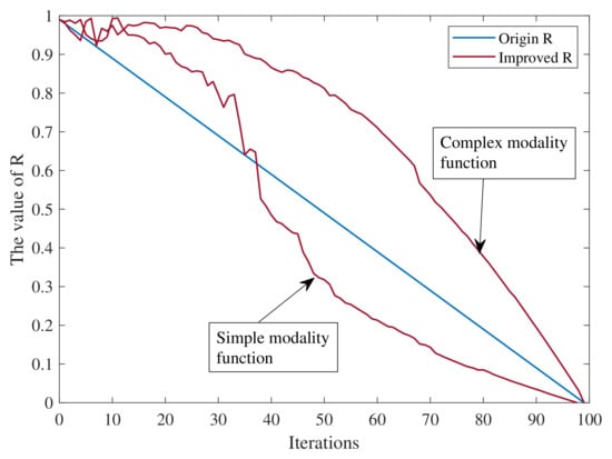
Figure 3.
Comparison of improved and original convergence factors R under different optimization scenarios.
Hybrid Mutation Based on Ruggedness
The original DBO algorithm faces challenges due to its limited convergence accuracy and a tendency to get trapped in local optima. Mutation operators are widely used to address these issues [32,33]. The choice of operator depends on the problem modality: for single-peak problems, the Gaussian mutation operator is typically chosen to facilitate faster convergence to the global optimum, while for multi-peak problems, the Cauchy mutation operator is preferred as it allows for better exploration around local optima.
However, varying capabilities are often desirable at different stages of the search process. The Cauchy–Gaussian mutation strategy, which employs a linear combination of Gaussian and Cauchy distributions, is a complementary approach designed to handle complex multi-peak scenarios [34]. The key challenge in hybrid mutation is determining the optimal coefficient that allows the mutation operator to best fit the current population. This optimal coefficient is dynamic and changes with the position of the population. In theory, such an optimal coefficient exists for each iteration. Thus, it is advantageous if the mixed strategy coefficients related to the given local fitness landscape can be self-determined.
Fitness landscapes bridge algorithms and their optimization problems, with ruggedness describing the complexity of these landscapes. To calculate the information entropy ruggedness, start with a population P consisting of L individuals, corresponding to a fitness value vector . Then, derive the differential sequence by
Define a symbolic function with respect to as
We obtain the sequence . The parameter is a constant, where a smaller increases sensitivity to the differences between neighboring fitness values.
The meanings of consecutively occurring symbols in are listed in Table 1. The entropic measure, based on the frequency of different symbol combinations in , is defined as
where is the frequency of two different sign values occurring consecutively in , and is the count of sub-blocks in . The logarithm base is six due to the six possible rugged shapes in Table 1, making a b-ary entropy measure ranging from 0 to 1. This measure indicates landscape complexity by quantifying the frequency of consecutive combinations of different symbol values in . The entropy is a measure of the amount of information, so the larger is, the greater the variety of combinations of consecutively different sign values in the sequence , and the more structure and ruggedness that the landscape contains. The smaller indicates that the sequence has a more homogeneous variety of combinations of consecutively different sign values, and the landscape contains less and smoother structure.

Table 1.
Classification and encoding of three-point objects.
For the same difference sequence , the measurement of its ruggedness is influenced by the size of , which determines the interval of the neutral region. The larger is, the larger the interval of the neutral region, equivalent to an observer viewing the local landscape from a distance, where many tiny undulations cannot be observed. In this case, provides a coarse-grained observation. Conversely, the smaller is, the closer the observer is to the local landscape, allowing for the observation of any small changes in the fitness values. Here, provides a fine-grained observation. The smallest value of for which the landscape becomes flat, i.e., for which is a string of zeros, is called the information stability measure and is denoted by [35]. The value of would therefore equate to the largest difference in fitness values between any two successive points on the path. Let be a set of values that gradually decrease, approaching zero, referred to as the information entropy ruggedness vector . Ruggedness is then defined in this paper as the mean of information entropy at multiple observation granularities, given by
An instinctive hybrid mutation strategy is employed as
where denotes a random number from the standard Gaussian distribution, and denotes a random number from the standard Cauchy distribution. If the local fitness landscape appears multi-modal, a higher coefficient for Cauchy mutation is used. Conversely, a higher coefficient for Gaussian mutation is used for unimodal landscapes. This approach adds a multiplicative term related to the current fitness landscape to the hybrid mutation term, enabling dung beetles to adaptively adjust and optimize effectively. This method prevents missing local optima due to the limitations of the Cauchy mutation or ignoring global searches due to the limitations of the Gaussian mutation, especially early in the process when the population is evenly distributed.
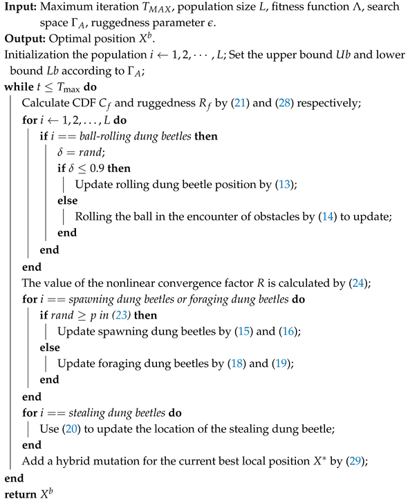
The implementation of the ADBO algorithm is shown in Algorithm 1.
| Algorithm 1: The ADBO algorithm |
 |
2.3.3. Convergence Performance Test
The convergence performance of the proposed ADBO algorithm is evaluated using the benchmark test functions from the 2020 IEEE Congress on Evolutionary Computation (CEC2020) [36], which are a collection of synthetic mathematical optimization problems widely used to evaluate the search efficiency and robustness of optimization algorithms. The characteristics of the functions are summarized in Table 2. Due to the limited variants of the DBO algorithm, we compare it with seven other popular swarm intelligence algorithms: PSO, GWO, PIO, HHO, SSA, PO, and the basic DBO.
Table 2.
Characteristics of CEC2020 test functions 1.
To ensure the fairness of the experiment, the initial population size for all algorithms is set to 30, the maximum number of iterations to 500, and the search dimension to 30. To eliminate randomness, the evaluation criteria used are the mean and standard deviation of the solution results. Each algorithm is independently run 100 times on each test function. The parameters for the comparison algorithms are listed in Table 3, with ADBO and DBO sharing the same parameter settings.
Table 3.
Parameters of swarm intelligence algorithms.
The experiments were conducted on a computer system with an Intel(R) i7-12700H CPU and 16 GB RAM running a 64-bit version of Microsoft Windows 11. The source code was implemented in the MATLAB (R2024a) programming environment. All subsequent experiments were performed on the same equipment.
Table 4 presents the mean, standard deviation, and ranking of the solution results for ADBO and the comparison algorithms across each function in CEC2020. The ranking of the eight algorithms prioritizes the mean value. As shown in Table 4, ADBO achieves the top rank (i.e., rank 1) on seven out of ten benchmark functions, based on the mean value of each algorithm’s results. It not only excels in unimodal and basic functions but also shows significant advantages in hybrid and composition functions. Notably, in , ADBO, HHO, and PO are effectively tied for first place, with minimal performance differences. In the first four functions, except for , where ADBO is not ranked first, it performs optimally in all other functions. ADBO secured the top ranking in all hybrid and composition functions, except for function , where PSO and SSA slightly outperformed it. These results demonstrate that ADBO consistently finds better solutions for these functions while maintaining high stability in its solutions. Overall, ADBO achieved the lowest total rank, indicating its superior performance compared with the other algorithms. In particular, ADBO not only offers significantly better solution accuracy than the original DBO algorithm but also exhibits lower variance. The effectiveness of these improvements is further validated by the Friedman mean rank test. As shown in Figure 4, ADBO consistently outperforms the other algorithms, thereby demonstrating the effectiveness of the improvements.
Table 4.
CEC2020 test results in 30-dimension.
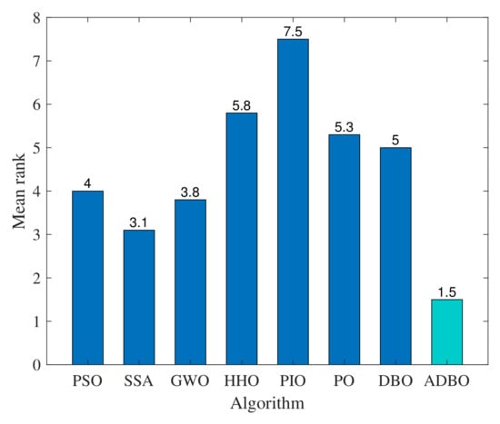
Figure 4.
Friedman mean rank test results.
The comparative convergence curves of the ADBO and seven other swarm intelligence algorithms are shown in Figure 5. These curves demonstrate that ADBO has a faster convergence rate than the other algorithms and can maintain a consistent search throughout the iterations, thereby reducing the likelihood of falling into local optima. The convergence curve of ADBO is also less volatile and stabilizes more effectively. Moreover, for most test functions, ADBO exhibits an accelerated convergence trend, indicating that its search capability enhances as iterations progress, allowing it to find better solutions more quickly. However, it is worth noting that on function , SSA outperforms ADBO, and on function , PSO, SSA, and GWO were able to match or even surpass ADBO in performance. Despite these exceptions, ADBO outperformed the other algorithms in the remaining functions tested. In summary, the comparison results demonstrate ADBO’s significant advantages in performance and its superiority across different types of problems, validating its overall effectiveness.
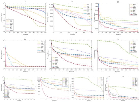
Figure 5.
CEC2020 iteration curve chart.
3. Experimental Results and Analysis
In this section, we apply our study to the optimization problem in DPE, conducting experiments with both simulated and real signals. For simplicity, in the following sections, the abbreviations for swarm intelligence algorithms will refer directly to their application in the DPE-SI framework.
3.1. Simulated Signal Experiments
In the simulated signal experiments, we conducted a comprehensive comparative analysis involving ten algorithms. Among them, we included the widely used traditional search algorithms, namely the ARS algorithm and the MRG algorithm. Additionally, we incorporated the seven popular swarm intelligence algorithms that were previously discussed in Section 2.3.3. Furthermore, a nonlinear weighted least squares method, known as 2SP, was utilized as a control algorithm to effectively verify the positioning performance. Two scenarios were considered: one with fine satellite geometry and another with poor satellite geometry. To maintain clarity and simplicity, assuming the receiver remained stationary, we focused only on position–time domain searches in both scenarios. Our analysis concentrated on a civilian GPS L1 signal, filtered with a 1 MHz bandwidth filter and sampled at MHz, using real ephemeris data for simulation. Atmospheric delays were modeled: ionospheric effects were simulated using the Klobuchar model, and tropospheric delays were represented using the Hopfield model [37]. The uncertainty space of the position was defined by the typical uncertainties of assistance data provided via GSM cellular networks: a horizontal uncertainty range of m and a vertical uncertainty range of m. The center of this uncertainty space deviates from the true position by m, m, and m in the Cartesian space, resulting in a total positional error of approximately m. Given the larger uncertainty range of the clock bias relative to the position uncertainty, the clock bias search was managed separately, with an uncertainty range set to m to facilitate the experiment [7]. Estimation performance was assessed using the root mean square errors of the estimated position, while computational cost was evaluated based on CPU processing time. The initial population size for each swarm intelligence algorithm was set to 100, with the remaining parameter settings kept consistent in Table 3. The grid step sizes for the MRG algorithm were summarized in Table 5 [12]. The number of iterations for the ARS algorithm was set equal to the total number of points in the MRG algorithm. To reduce the impact of randomness, each algorithm was independently run 50 times.
Table 5.
Description of the search space stage used in MRG.
3.1.1. Fine Satellite Geometry
We first consider an open-sky reception scenario with eight satellites, using a elevation mask at a of 30 dB/Hz. The corresponding PRN code numbers, azimuths, and elevations of the satellites are summarized in Table 6.
Table 6.
Azimuth and elevations of satellites with fine geometry.
The position error (PE), clock bias error (CBE), number of evaluated points (PN), and execution time (ET) of the ten algorithms were compared, as shown in Table 7. Due to fundamental differences in processing architecture between traditional 2SP and DPE, the execution time of 2SP is not included in the analysis. In 2SP, pseudoranges are first obtained through acquisition and tracking, followed by near real-time least-squares solving. In contrast, DPE directly estimates the position by correlating raw signals without intermediate measurements. Therefore, the analysis focuses on evaluating the efficiency of different search algorithms within the DPE framework. As demonstrated in Table 7, the MRG, ARS, GWO, DBO, and ADBO algorithms achieve comparable positioning performance to 2SP, highlighting the effectiveness of the proposed DPE-SI framework. However, even in this ideal case, 2SP still provides the best results. Achieving similar results with DPE-SI methods would likely require either a finer grid or an increase in the number of populations and iterations, though this comes with higher computational costs. Among the DPE-SI methods, GWO, DBO, and ADBO achieve comparable positioning accuracy to the MRG and ARS but require significantly fewer candidate points to evaluate. Grid-based methods involve exhaustive evaluation of fixed-resolution candidate points, while random search algorithms rely on sufficient iterations, making them computationally expensive. In contrast, swarm intelligence algorithms employ populations of agents that intelligently explore the search space, focusing on promising regions and avoiding unnecessary evaluations. This efficiency leads to a substantial reduction in computation time for DPE compared with MRG and ARS. Nonetheless, certain algorithms like PSO, HHO, SSA, and PIO are sensitive to zeros and often converge to an incorrect search space, typically the zero point in the optimization problem. Consequently, these algorithms yield similar positioning errors. On the other hand, the PO algorithm frequently produces large errors due to its tendency to fall into local optima, resulting in a relatively high average positioning error.
Table 7.
Performance comparison of different optimization algorithms with fine geometry.
To visually demonstrate the performance of the swarm intelligence algorithms, the convergence curves and positioning error curves are presented in Figure 6. According to the results in Figure 6a, PSO and SSA converge relatively slowly, whereas the other algorithms achieve low fitness values within as few as 50 iterations. This is consistent with previous findings that PSO and SSA are better suited for unimodal problems, whereas the PIO algorithm exhibits poorer overall performance. Unfortunately, the majority of algorithms, including PO and HHO, suffer from falling into local optima, leading to stagnation. The DBO algorithm demonstrates advantages over other swarm intelligence algorithms, showing fast convergence and being less likely to fall into local optima. Building on this foundation, ADBO significantly enhances performance compared with DBO, outperforming other algorithms in terms of search capability and achieving the lowest fitness value.
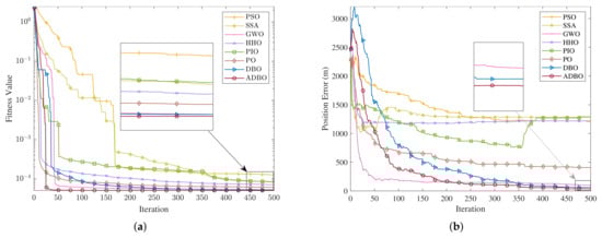
Figure 6.
Results of different algorithms under fine geometry. (a) Convergence curves. (b) Position errors curves.
It is worth noting that at the beginning of the search, ADBO’s fitness values do not decrease as quickly as those of other algorithms. This is because, for a complex search problem like DPE, FLA guides ADBO to prioritize a more global search initially, coupled with Gaussian mutation, rather than focusing on rapidly achieving lower fitness values locally. In the later stages of the search, ADBO shifts to favoring local search, incorporating Cauchy mutation to maintain continuous search capability. Consequently, ADBO tends to outperform other algorithms in obtaining the lowest fitness function value by the end of the iteration. As shown in Figure 6a, the convergence trends of the position error curve and the cost function curve are similar. However, due to the multi-peaked nature of the cost function in DPE, the position error curves do not continuously decrease like the convergence curves but instead fluctuate. This fluctuation occurs because the optimization problem in DPE essentially involves the correlation value between the signal corresponding to a candidate point and the true received signal. A candidate point achieves a smaller fitness value when some code phases are aligned and the global optimum when it aligns with all satellite code phases. This can result in situations where candidate points with smaller fitness values are actually further from the true position. By considering the fitness landscape of the cost function, the ADBO algorithm exhibits minimal fluctuation and the fastest convergence, demonstrating its superiority.
Due to the inherent randomness in population distribution during each independent experiment, the mean value of FDC and ruggedness appears as a gently declining curve, which does not clearly illustrate the relationship with the convergence curve of the fitness value. To better demonstrate this relationship, the convergence curve from a single experiment, along with the corresponding FDC and ruggedness curves, is shown in Figure 7. As shown in Figure 7b, at the beginning of the search, the initial population is randomly distributed, presenting lower values of and across a large search space. ADBO maintains a broad search range, promoting extensive exploration and foraging behavior. Around the 17th iteration, reaches its peak value, corresponding to a larger Cauchy mutation, which favors a more exhaustive search of the entire space. By the 61th iteration, rapidly decreases, and Gaussian mutation becomes more dominant. Despite the already low fitness value, FDC remains within the range of to until approximately the 265th iteration, enabling ADBO to retain its global search capability. This persistence is crucial in the DPE positioning problem, where even with individuals showing low fitness values, the FDC between individual populations remains high across the entire search space, indicating the problem’s deceptive nature. ADBO can adopt a suitable search strategy guided by FLA, which is unmatched by other algorithms. After this point, the value of begins to decline, significantly reducing the algorithm’s overall search space, with more emphasis on reproductive behavior and Gaussian mutation strategies. As seen in Figure 7a, in subsequent iterations, ADBO continues to effectively search for positions with smaller fitness values.
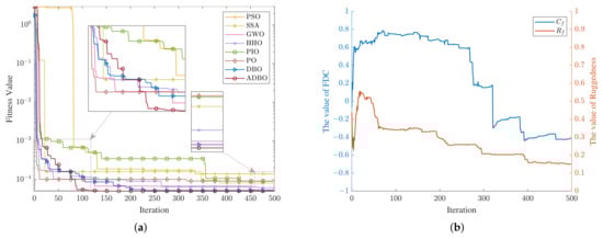
Figure 7.
Convergence curves, FDC, and ruggedness curves from a single experiment. (a) Convergence curves by different algorithms. (b) FDC and ruggedness curves.
3.1.2. Poor Satellite Geometry
It is well established that satellite geometry and signal strength significantly influence the multimodality of the cost function in DPE [3]. Poor satellite geometry increases the number of local optima within the search area, while lower signal strength raises the ratio of local optima to the global optimum, thereby increasing the search difficulty. To create a more challenging reception scenario, we simulated an indoor near-window environment characterized by poor satellite geometry and a low level of 25 dB/Hz. In this scenario, only satellites with elevations between and and azimuths between and were used. The corresponding PRN code numbers, azimuths, and elevations of the satellites are summarized in Table 8.
Table 8.
Azimuth and elevations of satellites with poor geometry.
The results are presented in Table 9. In harsh environments, the 2SP method exhibits the greatest decline in performance, as low and poor satellite geometry impair the accuracy of the acquisition and tracking process, resulting in lower positioning accuracy compared with DPE-SI methods. This demonstrates that the proposed framework retains the ability of DPE to handle weak signals [1]. Among the DPE methods, traditional search algorithms exhibit the most pronounced performance degradation under challenging conditions, which is consistent with their iterative design. As previously discussed in Section 2.1, the search space contains numerous secondary peaks, posing significant challenges for search-based methods such as ARS. Due to the necessity of reverting to the initial search radius multiple times, its search accuracy experiences a substantial decline. Similarly, MRG encounters the same set of challenges. In the strategy of MRG, the search is conducted iteratively, with the search center being relocated and the search boundaries reduced after each iteration. If the highest peak is excluded from the search space after adjustments, the search may fail to locate the receiver’s accurate position. In contrast, swarm intelligence algorithms search over a bounded set of real numbers, ensuring that the highest peak is always within the search space, thus overcoming the inherent limitations of traditional search algorithms. Additionally, these traditional search algorithms are computationally expensive, especially as the number of dimensions increases. Swarm intelligence algorithms, however, can control the number of points evaluated by adjusting the number of individuals and iterations, leading to more efficient and consistent performance. As observed, GWO, DBO, and ADBO all achieve better performance than traditional search algorithms in terms of precision, stability, and execution time. Notably, while ADBO and 2SP exhibit comparably high positioning accuracy under fine satellite geometry, the ADBO algorithm shows the smallest reduction in accuracy under poor satellite geometry, which can be attributed to its effective navigation solution search capability within DPE, allowing it to better exploit the advantages of the DPE-SI framework.
Table 9.
Performance comparison of different optimization algorithms with poor geometry.
Figure 8a shows the convergence curves of each algorithm with the number of iterations. As the number of local optima rises due to the deterioration of the peak states of the optimization problem, all algorithms require more iterations to converge. The values of the local optima and the global optimum become closer, increasing the likelihood that algorithms will get trapped in local optima. Without a suitable strategy, it is challenging for the population to escape these local optima and find the global optimum. Figure 8b shows the position error curves for different algorithms. Due to the more challenging optimization problem posed by poor geometry, the fitness values decrease while the corresponding positional errors increase. Many algorithms appear to converge successfully in the fitness function plots, but in reality, they only fall into local optima with large positional errors. The ADBO algorithm, equipped with the improved strategies, not only converges quickly but also effectively escapes local optima. Consequently, it successfully converges to the correct position, achieving the least positioning error.
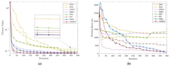
Figure 8.
Results of different algorithms under poor geometry. (a) Convergence curves. (b) Position errors curves.
3.2. Real Signal Experiments
To comprehensively validate the proposed method in real-world scenarios, we compared the single-point positioning performance of 2SP, MRG, and ADBO—identified as the top three algorithms based on their superior performance in simulation results shown in Table 7 and Table 9—under both fine and poor satellite geometry in the simulation experiments. It is worth noting that, unlike the simulation-based tests in Section 3.1, the following experiments rely solely on real GNSS signal data.
We used a NovAtel antenna and an OlinkStar GNSS signal record and playback instrument to collect raw intermediate frequency (IF) data. The GNSS signal recorder was configured to collect raw data at a MHz IF with 4-bit quantization. The sampling frequency was set to 25 MHz. The GNSS data collection equipment and the layout of the antennas are shown in the last subfigure of Figure 9.
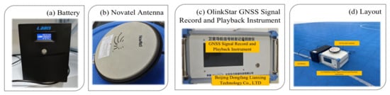
Figure 9.
Experiment setup of GNSS collection platform used for collecting GNSS datasets.
In the static receiver scenario, GNSS IF data were collected on 6 August 2019, at the West Playground of Huazhong University of Science and Technology in Wuhan, China. For the dynamic receiver scenario, data were collected on 11 June 2019, along Yujia Road at the same university. Both scenarios took place in an open-sky environment. In each scenario, a 40-s GPS L1 C/A dataset was collected, utilizing seven satellites for the analysis. The detailed specifications of the datasets are listed in Table 10 and Table 11, respectively.
Table 10.
Real test dataset parameters in static scenarios.
Table 11.
Real test dataset parameters in dynamic scenarios.
Additionally, the GNSS raw data were played back in a GNSS software-defined radio (v0.0.19.1), and the RINEX data, decimeter-level precision ground truth, and time reference were provided by post-processing and calibrated against the campus map. The positioning errors reported are measured against this reference, and the execution times represent the duration required for each individual positioning calculation. This prior information ensures accurate timing and helps simulate a typical uncertainty space, with a horizontal uncertainty range of m, a vertical uncertainty range of m, and a clock bias uncertainty range of m. Given the reduced space, the search precision of MRG is halved compared with the value specified in Table 5, resulting in a total of points to be evaluated. The weights for the 2SP method are derived from the values of each satellite. The population size for ADBO is set to 50, with a maximum of 100 iterations.
In the static receiver scenario, the sky plot and energy levels are shown in Figure 10a,b. Note that while some satellites (e.g., PRN 22) occasionally experienced slightly lower levels, most signals remained above 35 dB-Hz throughout the test duration. Each positioning calculation uses 1 ms of observation signals during the DPE correlation, corresponding to samples. The positioning results span from 2859 ms to ms, with calculations performed every 10 milliseconds, resulting in a total of 3714 positioning outcomes. Regarding the positioning performance, Figure 11a presents a planform map comparing the positioning results of the 2SP, MRG, and ADBO algorithms. The black cross symbol represents the ground truth (GT) position, while the blue dot, green circle, and red star represent the positioning results for 2SP, MRG, and ADBO, respectively. The results show that ADBO achieves slightly better positioning accuracy than 2SP, with MRG performing the worst. This indicates that the search capability of the MRG is insufficient under the current configuration, while ADBO remains effective.
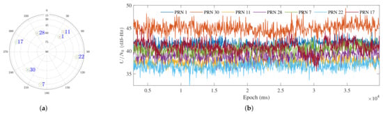
Figure 10.
Dataset Characteristics in the static receiver scenario. (a) Sky plot. (b) for each satellite.
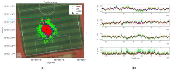
Figure 11.
Performance comparison of 2SP, ADBO, and MRG in the static receiver scenario. (a) Positioning platform map. (b) Comparison of positioning error.
Figure 11b shows the total positioning error () and the positioning errors of the three methods in the East (), North (), and up () directions. The blue, red, and green lines represent the positioning error curves for 2SP, ADBO, and MRG, respectively. The corresponding numerical results are summarized in Table 12.
Table 12.
Performance comparison in the static receiver scenario.
ADBO demonstrates significantly better search accuracy than MRG, with smaller positioning errors in all ENU directions. Specifically, ADBO reduces the total positioning error from m in MRG to m, achieving an improvement of approximately . The positioning errors in the ENU directions are reduced by , , and , respectively. Additionally, ADBO requires significantly less execution time than the MRG method, with a reduction from s to s, achieving an decrease in computational time. This is because ADBO evaluates far fewer candidate points than MRG. If higher accuracy is desired, the computational cost for MRG increases exponentially, making it impractical.
In the dynamic receiver scenario, the initial search space is configured identically to that in the static scenario. For each subsequent epoch, the algorithm centers the search space around the previous solution, with a search space size reduced to half of that in the static scenario. The sky plot and energy levels are shown in Figure 12a,b. While PRN 4 exhibits relatively lower and PRN 23 shows a noticeable signal attenuation between 25 s and 28 s, such variations are representative of realistic conditions in dynamic environments. The goal is to evaluate the algorithm’s robustness under challenges like signal fading and multipath. The positioning results span from 5978 ms to ms, resulting in a total of 3302 positioning outcomes.
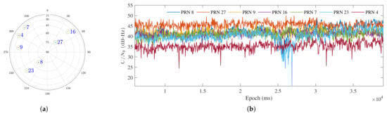
Figure 12.
Dataset Characteristics in the dynamic receiver scenario. (a) Sky plot. (b) for each satellite.
Figure 13a displays the road map of the positioning results, with the black line representing the true track and the blue, green, and red stars indicating the positioning results of the 2SP, MRG, and ADBO algorithms, respectively. Compared with 2SP and MRG, the positioning traces of ADBO exhibit higher accuracy and smaller fluctuations, demonstrating the ability of the proposed method to handle dynamic scenarios effectively. Figure 13b further illustrates the total positioning error and the positioning errors in the ENU directions for the three methods. It is evident that the MRG method performs relatively poorly, particularly around the middle of the experiment, where signal quality deteriorates. The corresponding numerical results are summarized in Table 13. Compared to the static reception scenario, 2SP experiences a greater degradation in positioning performance in the dynamic scenario than both MRG and ADBO, with reductions of , , and , respectively. ADBO still outperforms the MRG method with better positioning performance and lower computational cost. Specifically, ADBO reduces the total position error from m in MRG to m, achieving an improvement of approximately . The positioning errors in the ENU directions are also reduced by , , and , respectively. Moreover, ADBO dramatically decreases the execution time from s to s, resulting in an reduction in computational cost. These results indicate that the search capability of the MRG method is inadequate to realize the performance potential of DPE for the same computational cost, leading to lower positioning accuracy compared with the 2SP method. In contrast, the ADBO algorithm significantly accelerates the search process for navigation solutions, making it a more efficient solution for the DPE-SI framework.
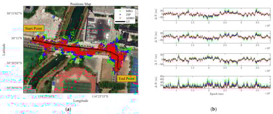
Figure 13.
Performance comparison of 2SP, ADBO, and MRG in the dynamic receiver scenario. (a) Positioning road map. (b) Comparison of positioning error.
Table 13.
Performance comparison in the dynamic receiver scenario.
4. Discussion
This study introduces a novel DPE framework that incorporates a low-complexity correlation approach combined with the ADBO algorithm to enhance positioning accuracy in complex environments while significantly reducing computational cost. Traditional 2SP methods face accuracy degradation in multipath and weak signal conditions. By leveraging global signal correlation and optimizing the search process through swarm intelligence, the proposed method effectively addresses these challenges. A key innovation is the integration of low-complexity correlation functions into the DPE framework, eliminating the need for full signal-level correlation. The ADBO algorithm, designed using FLA, dynamically adjusts the population structure and convergence factors, enhancing flexibility in the optimization process, particularly through a hybrid Cauchy–Gaussian mutation strategy.
Experimental results, including benchmark tests using CEC2020 functions, demonstrate that ADBO achieves superior convergence and optimization performance, ranking first among all comparative algorithms. The DPE-SI method consistently outperformed MRG, ARS, and 2SP in both fine and poor satellite geometries, improving positioning accuracy and computational efficiency. In real-world experiments, ADBO-based DPE achieved the highest positioning accuracy and reduced computational time by 82.1% and 85.8% in static and dynamic scenarios, respectively, compared with MRG. Despite promising results, several limitations remain. The iterative nature of ADBO results in higher runtime compared with 2SP, which could be a constraint for real-time applications. Additionally, the robustness of the proposed method under extremely low signal-to-noise ratio conditions or in highly multipath-prone environments was not assessed and warrants further investigation.
Future work will focus on optimizing real-time performance and exploring hardware-level acceleration. Furthermore, the DPE-SI framework will be extended to support multi-frequency, multi-constellation GNSS signals, enhancing its robustness and global applicability. Potential applications include urban canyon navigation, UAV high-dynamic positioning, and low-cost GNSS devices. In summary, this study demonstrates that integrating swarm intelligence with low-complexity correlation-based DPE enables high-precision positioning under challenging conditions while significantly reducing computational overhead.
5. Conclusions
This paper proposes the DPE-SI framework, integrating swarm intelligence algorithms with a low-complexity correlation strategy to efficiently solve the DPE problem. A novel ADBO algorithm based on FLA was developed to dynamically adjust its search strategy and incorporate a hybrid mutation strategy, enhancing both global and local search capabilities. Benchmark tests on CEC2020 functions demonstrate that ADBO outperforms conventional search methods and other swarm intelligence algorithms, with faster convergence and superior positioning accuracy. Simulation results show significant improvements in both convergence speed and positioning accuracy while reducing computational cost. Real-signal experiments confirm the algorithm’s robustness, with ADBO improving positioning accuracy by 9.6% over 2SP and 45.6% over MRG in static scenarios and 26.5% and 46.6% in dynamic scenarios, respectively. Computational time was reduced by 82.1% in static and 85.8% in dynamic tests. The combined DPE-SI framework and ADBO algorithm offer an efficient and accurate solution for GNSS positioning, showing significant potential for use in low-cost GNSS devices and applications with limited computational resources.
Author Contributions
Conceptualization, Y.D. and J.W.; Formal analysis, Z.T. and K.Y.; Investigation, Y.D. and Z.T.; Methodology, Y.D. and Z.T.; Software, Y.D. and K.Y.; Supervision, Z.T. and J.W.; Validation, Y.D., Z.T., J.W. and K.Y.; Visualization, J.S.; Writing—original draft, Y.D. and Z.T.; Writing—review and editing, Y.D., J.W. and J.S. All authors have read and agreed to the published version of the manuscript.
Funding
This research was funded by the National Natural Science Foundation of China (Nos. 62171191 and 62271223).
Data Availability Statement
The original contributions presented in the study are included in the article, further inquiries can be directed to the corresponding author.
Conflicts of Interest
The authors declare no conflicts of interest.
References
- Closas, P.; Gusi-Amigo, A. Direct Position Estimation of GNSS Receivers: Analyzing Main Results, Architectures, Enhancements, and Challenges. IEEE Signal Process. Mag. 2017, 34, 72–84. [Google Scholar] [CrossRef]
- Peretic, M.; Gao, G.X. Design of a Parallelized Direct Position Estimation-Based GNSS Receiver. NAVIGATION J. Inst. Navig. 2021, 68, 21–39. [Google Scholar] [CrossRef]
- Huang, J.; Yang, R.; Gao, W.; Zhan, X. Geometric Characterization on GNSS Direct Position Estimation in Navigation Domain. IEEE Trans. Aerosp. Electron. Syst. 2024, 60, 4105–4123. [Google Scholar] [CrossRef]
- Duan, Y.; Wei, J.; Tang, Z. Asymptotic Performance of GNSS Positioning Approaches under Cross-Correlation Effects. Remote Sens. 2024, 16, 1407. [Google Scholar] [CrossRef]
- Tang, S.; Li, H.; Calatrava, H.; Closas, P. Precise Direct Position Estimation: Validation Experiments. In Proceedings of the 2023 IEEE/ION Position, Location and Navigation Symposium, Monterey, CA, USA, 24–27 April 2023; pp. 911–916. [Google Scholar] [CrossRef]
- Closas, P.; Fernandez-prades, C.; Fernkndez-rubiot, J.A.; Nord, C. ML Estimation of Position in a GNSS Receiver Using the SAGE Algorithm. Acoust. Speech Signal Process. 2007, 1, 1045–1048. [Google Scholar] [CrossRef]
- Cheong, J.W.; Wu, J.; Dempster, A. Dichotomous Search of Coarse Time Error in Collective Detection for GPS Signal Acquisition. GPS Solut. 2015, 19, 61–72. [Google Scholar] [CrossRef]
- Li, H.; Tang, S.; Wu, P.; Closas, P. Robust Interference Mitigation Techniques for Direct Position Estimation. IEEE Trans. Aerosp. Electron. Syst. 2023, 59, 8969–8980. [Google Scholar] [CrossRef]
- Appel, M.J.; LaBarre, R.; Radulovic, D. On Accelerated Random Search. SIAM J. Optim. 2004, 14, 708–731. [Google Scholar] [CrossRef]
- Axelrad, P.; Bradley, B.K.; Donna, J.; Mitchell, M.; Mohiuddin, S. Collective Detection and Direct Positioning Using Multiple GNSS Satellites. Navig. J. Inst. Navig. 2011, 58, 305–321. [Google Scholar] [CrossRef]
- Li, L.; Cheong, J.W.; Wu, J.; Dempster, A.G. Improvement to Multi-Resolution Collective Detection in GNSS Receivers. J. Navig. 2014, 67, 277–293. [Google Scholar] [CrossRef]
- Narula, L.; Singh, K.P.; Petovello, M.G. Accelerated Collective Detection Technique for Weak GNSS Signal Environment. In Proceedings of the 2014 Ubiquitous Positioning Indoor Navigation and Location Based Service, Corpus Christi, TX, USA, 20–21 November 2014; pp. 81–89. [Google Scholar] [CrossRef]
- Vicenzo, S.; Xu, B.; Xu, H.; Hsu, L.T. GNSS Direct Position Estimation-Inspired Positioning with Pseudorange Correlogram for Urban Navigation. GPS Solut. 2024, 28, 83. [Google Scholar] [CrossRef]
- Jia, Z. A Type of Collective Detection Scheme with Improved Pigeon-Inspired Optimization. Int. J. Intell. Comput. Cybern. 2016, 9, 105–123. [Google Scholar] [CrossRef]
- Zhao, W.; Liu, G.; Wang, S.; Gao, M.; Lv, D. Real-Time Estimation of GPS-BDS Inter-System Biases: An Improved Particle Swarm Optimization Algorithm. Remote Sens. 2021, 13, 3214. [Google Scholar] [CrossRef]
- Chen, H.; Niu, F.; Su, X.; Geng, T.; Liu, Z.; Li, Q. Initial Results of Modeling and Improvement of BDS-2/GPS Broadcast Ephemeris Satellite Orbit Based on BP and PSO-BP Neural Networks. Remote Sens. 2021, 13, 4801. [Google Scholar] [CrossRef]
- Mirjalili, S.; Mirjalili, S.M.; Lewis, A. Grey Wolf Optimizer. Adv. Eng. Softw. 2014, 69, 46–61. [Google Scholar] [CrossRef]
- Heidari, A.A.; Mirjalili, S.; Faris, H.; Aljarah, I.; Mafarja, M.; Chen, H. Harris Hawks Optimization: Algorithm and Applications. Future Gener. Comput. Syst. 2019, 97, 849–872. [Google Scholar] [CrossRef]
- Xue, J.; Shen, B. A novel swarm intelligence optimization approach: Sparrow search algorithm. Syst. Sci. Control Eng. 2020, 8, 22–34. [Google Scholar] [CrossRef]
- Lian, J.; Hui, G.; Ma, L.; Zhu, T.; Wu, X.; Heidari, A.A.; Chen, Y.; Chen, H. Parrot Optimizer: Algorithm and Applications to Medical Problems. Comput. Biol. Med. 2024, 172, 108064. [Google Scholar] [CrossRef]
- Xue, J.; Shen, B. Dung Beetle Optimizer: A New Meta-Heuristic Algorithm for Global Optimization. J. Supercomput. 2023, 79, 7305–7336. [Google Scholar] [CrossRef]
- Ratnakumar, R.; Nanda, S.J. A High Speed Roller Dung Beetles Clustering Algorithm and Its Architecture for Real-Time Image Segmentation. Appl. Intell. 2021, 51, 4682–4713. [Google Scholar] [CrossRef]
- Quan, M.; Zhang, J.; Zhang, R. A Novel Rain Identification and Rain Intensity Classification Method for the CFOSAT Scatterometer. Remote Sens. 2024, 16, 887. [Google Scholar] [CrossRef]
- Zhu, F.; Li, G.; Tang, H.; Li, Y.; Lv, X.; Wang, X. Dung Beetle Optimization Algorithm Based on Quantum Computing and Multi-Strategy Fusion for Solving Engineering Problems. Expert Syst. Appl. 2024, 236, 121219. [Google Scholar] [CrossRef]
- Li, W.; Dong, Q.; Wang, B.; Xiang, M. A New Multi-Channel Triangular FMCW LADAR Signals Denoising Method Based on Improved SMVMD. Remote Sens. 2024, 16, 4650. [Google Scholar] [CrossRef]
- Wang, M.; Li, B.; Zhang, G.; Yao, X. Population Evolvability: Dynamic Fitness Landscape Analysis for Population-Based Metaheuristic Algorithms. IEEE Trans. Evol. Comput. 2018, 22, 550–563. [Google Scholar] [CrossRef]
- Coric, R.; Dumic, M.; Jakobovic, D. Genetic Programming Hyperheuristic Parameter Configuration Using Fitness Landscape Analysis. Appl. Intell. 2021, 51, 7402–7426. [Google Scholar] [CrossRef]
- Weill, L.R. A High Performance Code and Carrier Tracking Architecture for Ground-Based Mobile GNSS Receivers. In Proceedings of the 23rd International Technical Meeting of the Satellite Division of The Institute of Navigation, Portland, OR, USA, 21–24 September 2010; pp. 3054–3068. [Google Scholar]
- Vincent, F.; Chaumette, E.; Charbonnieras, C.; Israel, J.; Aubault, M.; Barbiero, F. Asymptotically Efficient GNSS Trilateration. Signal Process. 2017, 133, 270–277. [Google Scholar] [CrossRef]
- Tay, S.; Marais, J. Weighting Models for GPS Pseudorange Observations for Land Transportation in Urban Canyons. In Proceedings of the 6th European Workshop on GNSS Signals and Signal Processing, Munich, Germany, 5–6 December 2013; Available online: https://hal.science/hal-00942180 (accessed on 15 May 2025).
- Shen, L.; He, J. A Mixed Strategy for Evolutionary Programming Based on Local Fitness Landscape. In Proceedings of the IEEE Congress on Evolutionary Computation, Barcelona, Spain, 18–23 July 2010; pp. 1–8. [Google Scholar] [CrossRef]
- Hua, B.; Yang, G.; Wu, Y.; Chen, Z. Path Planning of Spacecraft Cluster Orbit Reconstruction Based on ALPIO. Remote Sens. 2022, 14, 4768. [Google Scholar] [CrossRef]
- Gupta, S.; Su, R. An Efficient Differential Evolution with Fitness-Based Dynamic Mutation Strategy and Control Parameters. Knowl.-Based Syst. 2022, 251, 109280. [Google Scholar] [CrossRef]
- Gong, C.; Wu, D.; Jiang, L.; Dong, F.; Liu, J.; Chen, Y.; Cao, J.; Wang, D. Seizure Detection Algorithm Based on Multidimensional Covariance Matrix and Binary Harris Hawks Optimization With Cauchy–Gaussian Mutation. IEEE Sens. J. 2024, 24, 4596–4608. [Google Scholar] [CrossRef]
- Malan, K.M.; Engelbrecht, A.P. Quantifying Ruggedness of Continuous Landscapes Using Entropy. In Proceedings of the 2009 IEEE Congress on Evolutionary Computation, Trondheim, Norway, 18–21 May 2009; pp. 1440–1447. [Google Scholar] [CrossRef]
- Liang, J.J.; Suganthan P., N.; Qu, B.; Gong, D.; Yue, C. Problem Definitions and Evaluation Criteria for the CEC 2020 Special Session on Multimodal Multiobjective Optimization; Computational Intelligence Laboratory, Zhengzhou University: Zhengzhou, China, 2019; pp. 353–370. [Google Scholar] [CrossRef]
- Chiang, K.W.; Duong, T.T.; Liao, J.K. The Performance Analysis of a Real-Time Integrated INS/GPS Vehicle Navigation System with Abnormal GPS Measurement Elimination. Sensors 2013, 13, 10599–10622. [Google Scholar] [CrossRef]
Disclaimer/Publisher’s Note: The statements, opinions and data contained in all publications are solely those of the individual author(s) and contributor(s) and not of MDPI and/or the editor(s). MDPI and/or the editor(s) disclaim responsibility for any injury to people or property resulting from any ideas, methods, instructions or products referred to in the content. |
© 2025 by the authors. Licensee MDPI, Basel, Switzerland. This article is an open access article distributed under the terms and conditions of the Creative Commons Attribution (CC BY) license (https://creativecommons.org/licenses/by/4.0/).