Codesign of Transmit Waveform and Receive Filter with Similarity Constraints for FDA-MIMO Radar

Abstract

The codesign of the receive filter and transmit waveform under similarity constraints is one of the key technologies in frequency diverse array multiple-input multiple-output (FDA-MIMO) radar systems. This paper discusses the design of constant modulus waveforms and filters aimed at maximizing the signal-to-interference-and-noise ratio (SINR). The problem’s non-convexity renders it challenging to solve. Existing studies have typically employed relaxation-based methods, which inevitably introduce relaxation errors that degrade system performance. To address these issues, we propose an optimization framework based on the joint complex circle manifold–complex sphere manifold space (JCCM-CSMS). Firstly, the similarity constraint is converted into the penalty term in the objective function using an adaptive penalty strategy. Then, JCCM-CSMS is constructed to satisfy the waveform constant modulus constraint and filter norm constraint. The problem is projected into it and transformed into an unconstrained optimization problem. Finally, the Riemannian limited-memory Broyden–Fletcher–Goldfarb–Shanno (RL-BFGS) algorithm is employed to optimize the variables in parallel. Simulation results demonstrate that our method achieves a 0.6 dB improvement in SINR compared to existing methods while maintaining competitive computational efficiency. Additionally, waveform similarity was also analyzed.

1. Introduction

The codesign of the receive filter and transmit waveform is one of the key technologies in frequency diverse array multiple-input multiple-output (FDA-MIMO) radar systems. Frequency diverse array (FDA) radar applies different frequency offsets to the transmitting antenna, and the phase of the echo signal contains distance information, which effectively increases the degree of freedom of the distance dimension. Combined with the advantages of waveform diversity of MIMO radar, FDA-MIMO radar has advantages such as enhancing the system’s anti-interference performance and achieving more accurate target identification [1,2,3,4,5,6,7]. Therefore, the research on FDA-MIMO-related technologies has received extensive attention in recent years. For example, the joint design of the transmitter and the receiver can help further improve the system performance through collaborative optimization and mutual cooperation, so it has become one of the main research directions of FDA-MIMO radar.

We modeled the joint design problem of the transmit waveform and the receive filter to maximize the signal-to-interference-and-noise ratio (SINR) of the received signal. On this basis, similarity constraints and constant modulus constraints are imposed on the waveform. The constant modulus waveform can not only maximize the energy efficiency of the power amplifier but also effectively avoid nonlinear distortion [8,9,10]. The similarity constraint ensures that the designed waveform retains some favorable characteristics, such as low sidelobe characteristics and good autocorrelation characteristics, by selecting an appropriate reference waveform [11,12,13,14]. However, this optimization problem is non-convex, which presents significant challenges in finding a solution.

Most of the existing methods for non-convex joint optimization problems in FDA-MIMO radar system are based on a relaxation strategy and can be classified into two main categories. The first category of methods employs a two-stage optimization strategy. The second category of methods employs an alternating iterative optimization strategy.

In the first category of methods, the initial stage entails deriving the expression for the receive filter using the minimum variance distortionless response (MVDR) algorithm, which is substituted into the optimization problem to optimize the waveform [15,16,17]. In [15], the semidefinite relaxation (SDR) method is proposed for addressing the transmit waveform design problem under similarity constraints. This approach involves matrix inversion and decomposition operations, resulting in relatively high computational complexity [18,19]. Meanwhile, in [16], a method that utilizes the alternating direction method of multipliers (ADMM) is proposed to enhance the SINR while adhering to constraints on the similarity of transmit waveforms. This approach incorporates relaxation variables to convert the complex optimization problem into several tractable subproblems. To fully improve the transmitter’s efficiency, a constant modulus waveform optimization method based on ADMM has been proposed [17]. In the second stage, the expression is utilized to derive the receive filter. However, such methods struggle to fully explore the system’s performance potential due to their neglect of the interplay between variables during the optimization process.

In the second category of methods, the receiving filter and the transmitted waveform are alternately optimized during each iteration of the optimization process. This class of methods is currently a focal point of research. Refs. [17,20,21,22] all utilize the MVDR criterion to optimize the filter in each iteration. Refs. [20,23] introduced a transmit waveform optimization approach based on the majorization-minimization (MM) algorithm. The method simplifies the problem by relaxing the objective function into a surrogate function, thereby enhancing solvability. Nonetheless, constructing a suitable surrogate function is difficult. Ref. [21] proposed an efficient ADMM-based method to maximize the SINR under both peak-to-average power ratio (PAPR) constraints and similarity constraints. Although the PAPR constraint on the waveform can effectively prevent nonlinear distortion of the transmitter’s power amplifier, it will reduce the power utilization efficiency of the transmitter. To solve this problem, ref. [22] proposed an ADMM-based approach to jointly design constant modulus waveform and filters in an integrated sensing and communication system. Therefore, this problem can be studied in an FDA-MIMO radar system. However, ADMM is highly sensitive to the penalty parameter, so selecting an appropriate penalty factor is a challenging task [24].

The aforementioned methods are all based on relaxing the original problem, which inevitably introduces relaxation errors and leads to performance degradation. To address the aforementioned issues, we suggest a technique that relies on the joint complex circle manifold–complex sphere manifold space (JCCM-CSMS), which resolves the problem of the codesign of the constant modulus waveform and receive filters under the similarity constraint for FDA-MIMO radar. The specific procedure is as follows: First, an adaptive penalty strategy is employed to incorporate the similarity constraints into the objective function. Next, the JCCM-CSMS is constructed to transform the problem into an unconstrained optimization problem. Finally, the Riemannian limited-memory Broyden–Fletcher–Goldfarb–Shanno (RL-BFGS) algorithm [25] is utilized to achieve parallel solutions for both. This research presents several important contributions, detailed as follows:

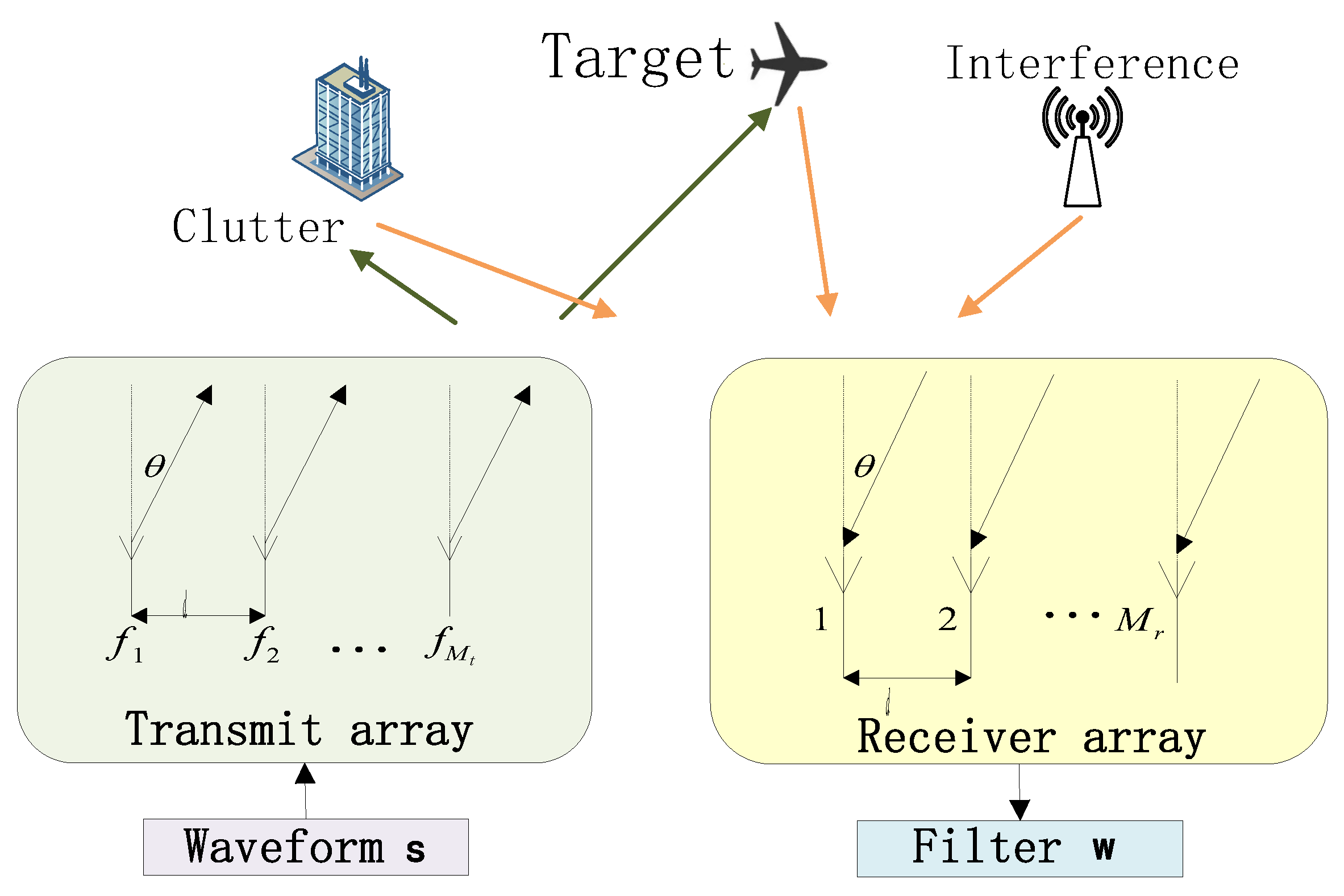
• The codesign model for constant modulus transmit waveforms and receive filters in FDA-MIMO radar
  In the existing research on waveform design of FDA-MIMO systems, peak-to-average power ratio (PAPR) and total energy constraints are usually considered [20,21]. The total energy constraint is mainly used to control resource costs, while the peak-to-average power ratio constraint avoids nonlinear distortion of the transmitter amplifier while controlling resource costs, but this constraint will also reduce the energy efficiency of the power amplifier. To solve this problem, this paper models the problem as maximizing the signal-to-interference ratio (SINR) of the system under the similarity constraint of the transmitted waveform, the constant modulus constraint, and the norm constraint of the receiving filter. While improving the system performance, it also ensures that the power amplifier maximizes energy efficiency while avoiding distortion and maintaining the excellent characteristics of the reference waveform.
• The adaptive penalty strategy
  Mainstream methods typically use penalty-based strategies to transform similarity constraints. However, most existing methods use fixed penalty factors [13,21,26,27], and selecting an appropriate penalty factor is challenging. A small penalty factor may result in the failure to meet the similarity constraint, while an excessively large penalty factor may significantly degrade system performance. To address this problem, we propose an optimization method based on an adaptive penalty factor. This method starts with a small penalty factor and gradually increases it during the iteration process until it reaches a suitable level. This allows the similarity constraint to be accurately met, maximizing the system’s optimization performance.
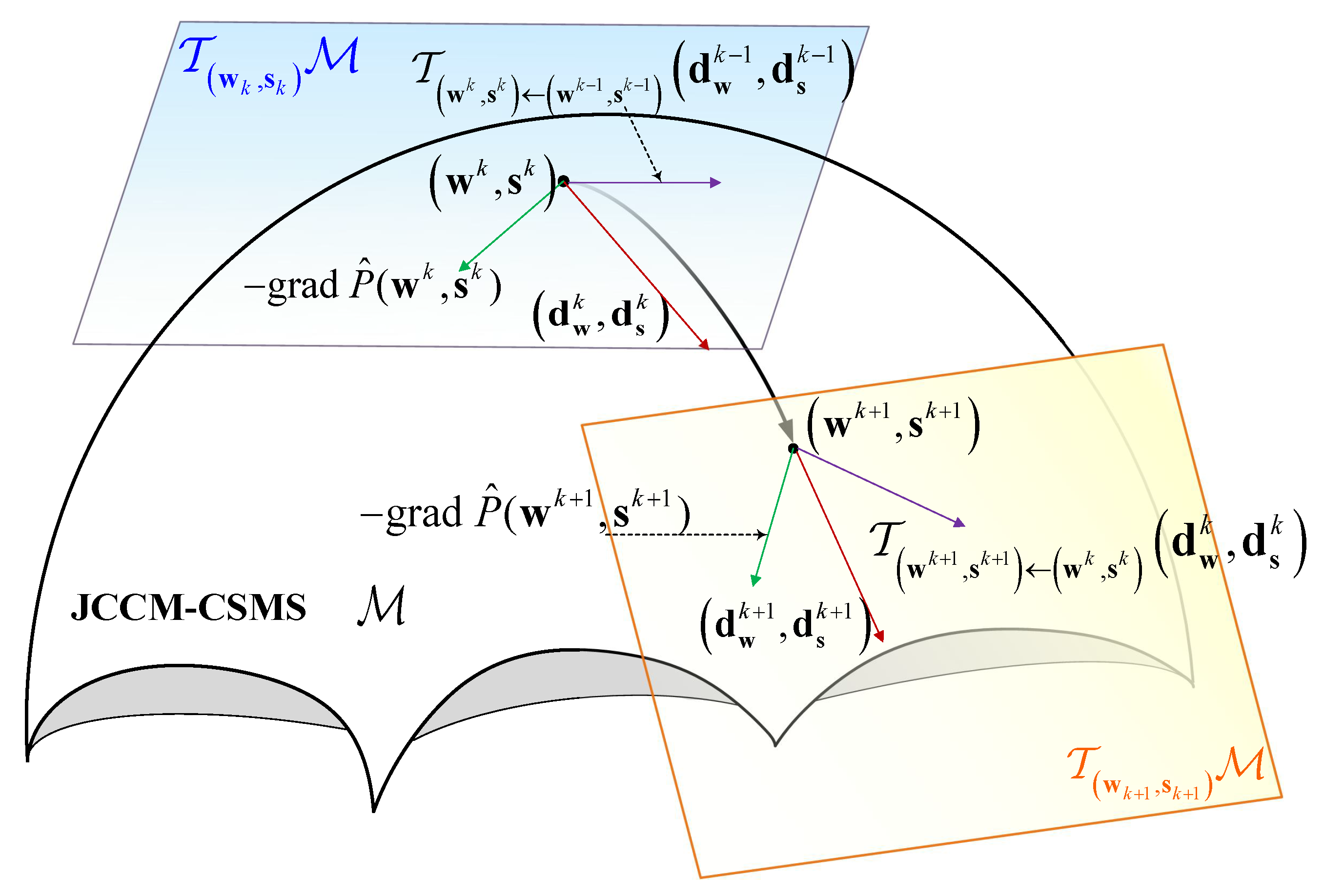
• The joint optimization method based on JCCM-CSMS
  The existing methods addressing the joint design problem of FDA-MIMO radar typically rely on relaxation strategies [17,20,21]. Relaxation transforms an otherwise difficult-to-solve optimization problem into a more tractable form; however, this process inevitably introduces errors, leading to performance loss. We have observed that the complex circle manifold space (CCMS) consists of complex vectors with unit modulus, while the complex sphere manifold space (CSMS) is composed of complex vectors with unit norm. Based on this observation, this paper constructs a joint space of the two, i.e., JCCM-CSMS. Through the projecting of the optimization problem into JCCM-CSMS, the original problem is converted into an unconstrained optimization problem, where the SINR takes the form of a quadratic fractional function that can be optimized using a classic gradient-based algorithm. Therefore, this method eliminates the need for relaxation, avoiding the errors introduced by relaxation and significantly improving optimization performance.
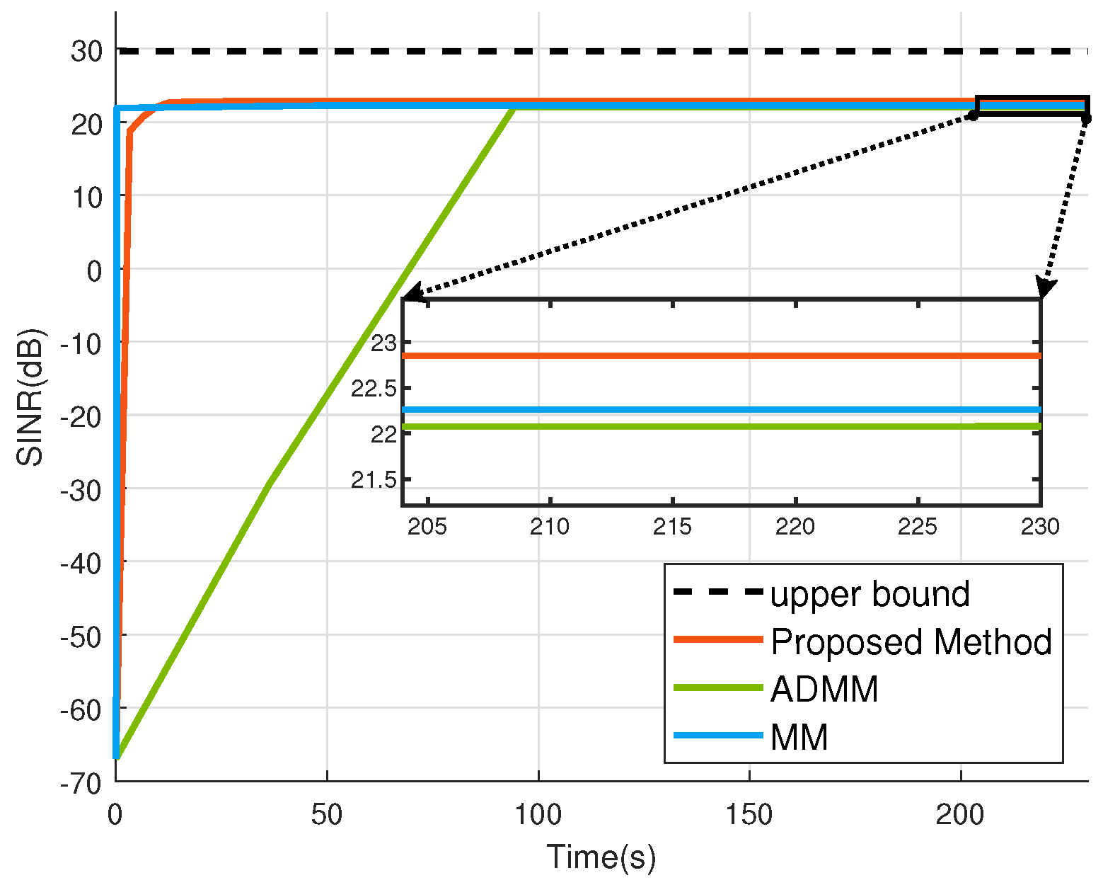
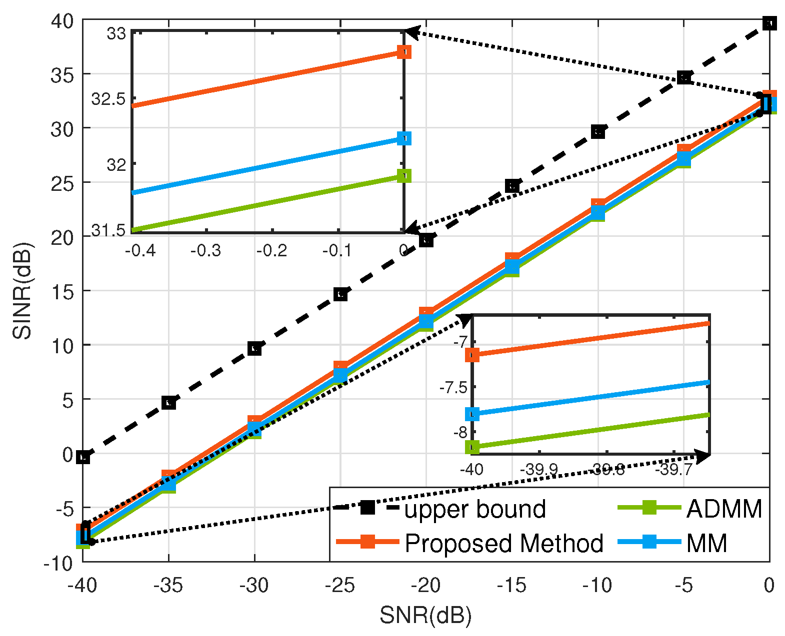
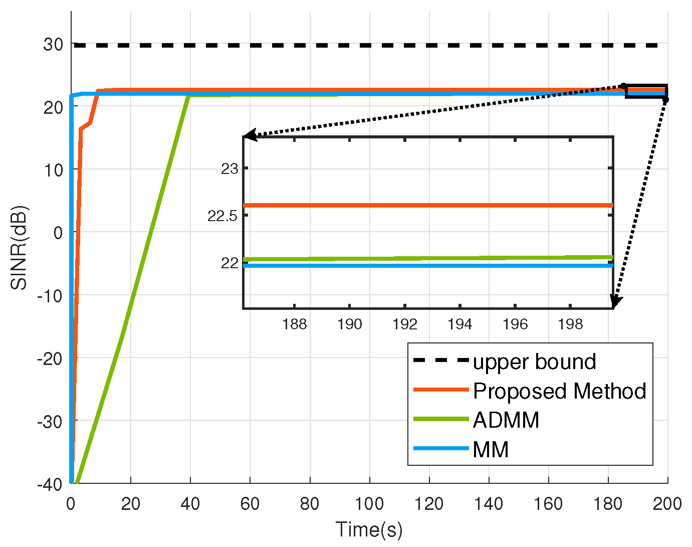
• Superior performance
  Simulation results show that the proposed method improves the SINR performance by about 0.7 dB compared with the ADMM-based method proposed in [22]. The performance of the proposed method is improved by about 0.6 dB compared with the MM-based method proposed in [23]. Improving the SINR of the received signal helps improve the accuracy of subsequent target detection and parameter estimation [28,29].

The structure of this paper is outlined as follows. In Section 2, we introduce the FDA-MIMO system model in the presence of interference and clutter, along with the proposed codesign framework for transmit waveforms and receive filters. Section 3 offers a detailed derivation of the joint optimization approach grounded in JCCM-CSMS. Section 4 demonstrates the performance of our proposed method through MATLAB R2024a simulations. Lastly, the conclusions can be found in Section 5.

${\parallel ·\parallel }_2$ represents the Euclidean norm. $\left|·\right|$ represents the modulus of a number. ${\left(·\right)}^T$ and ${\left(·\right)}^H$ represent the transpose operation and conjugate transpose operation of a matrix or vector, respectively. ${\left(·\right)}^{*}$ represents the conjugation of all elements in a vector or matrix. ⊙ is the Hadamard product between matrices or vectors, and ⊗ is the Kronecker product between matrices or vectors. $vec(·)$ represents the vectorization operation of the matrix; that is, the stacking of the columns of the matrix in order into a column vector. ${\mathbf{I}}_X$ represents the $X\times X$ dimensional identity matrix. $\Re \left(·\right)$ refers to taking the real part of a complex number/complex vector/complex matrix.

2. Problem Description

2.1. Signal Model

In a co-located FDA-MIMO radar system featuring uniform linear arrays (ULA) for both the transmitting and receiving antennas, the inter-element spacing between each antenna is half a wavelength. The system comprises $M_t$ transmitting antennas and $M_r$ receiving antennas, and the structure of the system is shown in Figure 1. The signal emitted by the m-th transmitting antenna can be represented as follows:

$$x_m\left(t\right)={\alpha }_m{s}_m\left(t\right)e^{j2\pi f_{m}t}$$

(1)

where ${\alpha }_m$ represents the weight of the antenna energy distribution, and $s_m\left(t\right)$ represents the baseband waveform transmitted by the m-th antenna, where $m=1,\cdots ,M_t$. The carrier frequency for each antenna is as follows [30,31,32,33]:

$$f_m=f_0+(m-1)△f,m=1,\cdots ,M_t$$

(2)

where $f_0$ denotes the carrier frequency of the first antenna, while $\Delta f$ represent the frequency offset occurring among the antennas. In the presence of K independent interference signals and Q correlated clutter scenarios, the target direction is ${\theta }_t$, with a distance of $r_t$. The q-th clutter direction is denoted as ${\theta }_{c,q}$, with distance $r_{c,q}$ for $q=1,\dots ,Q$, and the k-th interference direction is represented by ${\theta }_{j,k}$ for $k=1,\dots ,K$. Additionally, let the transmit vector of $M_t$ antennas at time l be $\mathbf{s}\left(l\right)={[s_1\left(l\right),s_2\left(l\right),\dots ,s_{M_t}\left(l\right)]}^T\in {\mathbb{C}}^{M_t\times 1}$. The received signal at discrete time l (where $l=1,\dots ,L$) is given by the following:

$${\mathbf{y}}_l={\beta }_t{\mathbf{\alpha }}_r\left(\theta \right){\mathbf{\alpha }}_t^T(r,\theta )\mathbf{s}\left(l\right)+\sum _{k=1}^K{\beta }_{j,k}{\mathbf{\alpha }}_r\left({\theta }_{j,k}\right){\tilde{\mathit{s}}}_{j,k}+\sum _{q=1}^Q{\beta }_{c,q}{\mathbf{\alpha }}_r\left({\theta }_{c,q}\right){\mathbf{\alpha }}_t^T(r_{c,q},{\theta }_{c,q})\mathbf{s}\left(l\right)+{\mathbf{n}}_l$$

(3)

where ${\tilde{\mathit{s}}}_{j,k}$ represents the zero-mean Gaussian distribution interference signal emitted from the k-th interference source, and ${\mathbf{n}}_l$ represents Gaussian white noise, which is commonly assumed in radar system models [34]. ${\mathbf{\alpha }}_t(r,\theta )$ and ${\mathbf{\alpha }}_r\left(\theta \right)$ denote the steering vectors for transmission and reception, respectively [35,36,37,38]:

$${\mathbf{\alpha }}_t(r,\theta )={[1,e^{j2\pi (\frac{2△fr}{c}-\frac{dsin\theta }{\lambda })},\cdots ,e^{j2\pi (M_t-1)(\frac{2△fr}{c}-\frac{dsin\theta }{\lambda })}]}^T$$

(4)

$${\mathbf{a}}_r\left(\theta \right)={[1,e^{-j2\pi \frac{dsin\theta }{\lambda }},\cdots ,e^{-j2\pi \left(M_r-1\right)\frac{dsin\theta }{\lambda }}]}^T$$

(5)

stack ${\mathbf{y}}_1,\dots ,{\mathbf{y}}_L$ into a single column vector:

$$\mathbf{y}={\beta }_t({\mathbf{S}}^T\otimes {\mathbf{I}}_{M_r})\mathbf{v}(r,\theta )+\sum _{k=1}^K{\beta }_{j,k}[{\tilde{\mathbf{s}}}_{j,k}\otimes {\mathbf{\alpha }}_r\left({\theta }_{j,k}\right)]+\sum _{q=1}^Q{\beta }_{c,q}({\mathbf{S}}^T\otimes {\mathbf{I}}_{M_r})\mathbf{v}(r_{c,q},{\theta }_{c,q})+\mathbf{n}$$

(6)

where $\mathbf{S}=\left[\mathbf{s}\left(1\right),\mathbf{s}\left(2\right),\dots ,\mathbf{s}\left(L\right)\right]\in {\mathbb{C}}^{M_t\times L}$ represents the transmit waveform matrix, and $\mathbf{v}(r,\theta )={\mathbf{a}}_t(r,\theta )\otimes {\mathbf{a}}_r\left(\theta \right)$. Let $\tilde{\mathbf{S}}=\mathbf{S}\otimes {\mathbf{I}}_{M_r}$. For target detection, beamforming is required under the assumption that the received signal is processed through the receiver filter $\mathbf{w}\in {\mathbb{C}}^{M_{r}L\times 1}$:

$$y^{\prime }={\mathbf{w}}^H\mathbf{y}$$

(7)

The resulting SINR can be expressed as follows [21]:

$$SINR\left(\mathbf{w},\mathbf{S}\right)=\frac{\mathbb{E}\left({|{\beta }_t{\mathbf{w}}^H\tilde{\mathbf{S}}\mathbf{v}\left(r,\theta \right)|}^2\right)}{{\mathbf{w}}^H\mathbb{E}\left({\mathbf{y}}_c{\mathbf{y}}_c^H+{\mathbf{y}}_j{\mathbf{y}}_j^H+\mathbf{n}{\mathbf{n}}^H\right)\mathbf{w}}$$

(8)

where $\mathbb{E}\left(\right|{\beta }_t{|}^2)={\delta }_t^2$, $\mathbb{E}\left(\right|{\beta }_{c,q}{|}^2)={\delta }_{c,q}^2$, $\mathbb{E}\left(\right|{\beta }_{j,k}{|}^2)={\delta }_{j,k}^2$, ${\delta }_n^2$ representing the target power, clutter power, interference power, and noise power, respectively. To express this more concisely, the SINR is typically represented using the covariance matrix. The covariance matrix of clutter and interference can be defined as follows:

$${\mathbf{R}}_c=\mathbb{E}\left({\mathbf{y}}_c{\mathbf{y}}_c^H\right)=\sum _{q=1}^Q{\delta }_{c,q}^2\tilde{\mathbf{S}}\mathbf{v}\left(r_{c,q},{\theta }_{c,q}\right){\mathbf{v}}^H\left(r_{c,q},{\theta }_{c,q}\right){\tilde{\mathbf{S}}}^H$$

(9)

$${\mathbf{R}}_j=\mathbb{E}\left({\mathbf{y}}_j{\mathbf{y}}_j^H\right)=\sum _{k=1}^K{\delta }_{j,k}^2\left[{\mathbf{I}}_k\otimes \left({\mathbf{a}}_r\left({\theta }_{j,k}\right){\mathbf{a}}_r^H\left({\theta }_{j,k}\right)\right)\right]$$

(10)

The SINR can be reformulated as follows:

$$SINR(\mathbf{w},\mathbf{S})=\frac{{\delta }_t^2{\left|{\mathbf{w}}^H\tilde{\mathbf{S}}\mathbf{v}(r,\theta )\right|}^2}{{\mathbf{w}}^H({\mathbf{R}}_c+{\mathbf{R}}_j+{\mathbf{R}}_n)\mathbf{w}}$$

(11)

2.2. Problem Modeling

2.2.1. Similarity Constraint

Although maximizing the SINR can improve subsequent processing performance to some extent [39], generating waveforms with desirable characteristics, such as good autocorrelation properties, is still necessary to further enhance resolution, localization accuracy, and other performance aspects. Radar systems require waveforms with favorable properties, as these characteristics are crucial for subsequent parameter estimation, target tracking, and classification [40]. A common approach in the literature involves implementing similarity constraints, which ensure that the designed waveform closely resembles a reference waveform with ideal properties. In radar systems, the distinction between the emitted waveform and the reference waveform is typically represented using the ${\ell }_2$ norm, defined as follows:  

$$\left|\right|\mathbf{s}-{\mathbf{s}}_0{\left|\right|}_2^2\le \xi$$

(12)

In this study, we select a orthogonal linear frequency modulation signal as the reference signal ${\mathbf{s}}_0$ to ensure that the waveform exhibits good autocorrelation properties [41,42,43].

2.2.2. Constant Modulus Constraint

In practical scenarios, constant modulus waveforms are frequently used to ensure the amplifiers operate at maximum efficiency while avoiding nonlinear distortion [9,44,45]. Therefore, we apply a constant modulus constraint to the transmitted waveform, defined as follows:

$$|s_m\left(l\right)|=\sqrt{p},l=1,\cdots ,L;m=1,\cdots ,M_t$$

(13)

2.2.3. Problem Model

In summary, the problem model is as follows:

$$\begin{array}{cc}\hfill {\mathcal{P}}_1:\underset{\mathbf{w},\mathbf{S}}{min}& f(\mathbf{w},\mathbf{S})=\frac{1}{SINR\left(\mathbf{w},\mathbf{S}\right)}\hfill \\ \hfill s.t.& |s_m\left(l\right)|=1,l=1,\cdots ,L;m=1,\cdots ,M_t\hfill \\ \hfill & \left|\right|\mathbf{s}-{\mathbf{s}}_0{\left|\right|}_2^2\le \xi \hfill \\ \hfill & {\left|\right|\mathbf{w}\left|\right|}_2^2=1\hfill \end{array}$$

(14)

where $\mathbf{s}=vec\left(\mathbf{S}\right)\in {\mathbb{C}}^{M_{t}L\times 1}$.

This problem is non-convex, and its solution process is highly challenging. Currently, most of the existing solution methods are relaxation-based. However, such relaxation methods inevitably introduce relaxation errors. In light of this, we propose a method based on JCCM-CSMS, which can effectively avoid the relaxation operation.

3. The Proposed Method

We propose a co-optimization method for the transmit waveform and the receive filter without relaxation in this section. Through the construction of a JCCM-CSMS that naturally satisfies the constant modulus constraint and the norm constraint, the problem is transformed into a more easily solvable unconstrained problem. Then, the RL-BFGS algorithm is utilized to perform parallel optimization on both of them. This avoids relaxation errors and reduces the computational time.

3.1. Adaptive Exact Penalty Method

This section first describes the application of the adaptive exact penalty algorithm to transform the problem:

$$\begin{array}{cc}\hfill {\mathcal{P}}_2:\underset{\mathbf{w},\mathbf{s}}{min}& Q(\mathbf{w},\mathbf{s})=f(\mathbf{w},\mathbf{s})+\kappa \left(max\{0,g(\mathbf{s}\left)\right\}\right)\hfill \\ \hfill s.t.& |s_m\left(l\right)|=1,l=1,...,L;m=1,\cdots ,M_t\hfill \\ \hfill & {\left|\right|\mathbf{w}\left|\right|}_2^2=1\hfill \end{array}$$

(15)

Here, $g\left(\mathbf{s}\right)=\parallel \mathbf{s}-{\mathbf{s}}_0{\parallel }_2^2-\xi ,\kappa >0$ is the penalty parameter. To address the non-differentiability of the max function, the log-sum-exp function can be utilized for smoothing. The relationship between the two is given by the following:

$$max\{a,b\}\approx ulog\left(e^{a/u}+e^{b/u}\right)$$

(16)

Let $u>0$ be the smoothing factor. The smoothing factor is decreased proportionally by ${\omega }_u\in (0,1)$ with each iteration until it reaches a predetermined minimum value $u_{min}$, i.e.:

$$u_{n+1}=max\left(u_{min},{\omega }_u{u}_n\right)$$

(17)

It can be observed that $\kappa$ increases adaptively during the iteration process. When $\kappa$ exceeds the threshold ${\kappa }_{max}$, the optimal solution of the penalty optimization problem ${\mathcal{P}}_2$ will converge to the optimal solution of the original problem ${\mathcal{P}}_1$. Directly selecting a larger penalty factor will result in a larger objective function loss, so a smaller penalty factor ${\kappa }_0$ is selected at the beginning of the iteration. When $g\left(\mathbf{s}\right)\ge u$, the constraint is considered not satisfied, and the penalty factor needs to be further increased:

$${\kappa }_{n+1}=\frac{{\kappa }_n}{{\omega }_{\kappa }}$$

(18)

where ${\omega }_{\kappa }\in (0,1)$.

By leveraging the properties discussed earlier, the problem can be further subsequently expressed as follows:

$$\begin{array}{cc}\hfill \underset{\mathbf{w},\mathbf{S}}{min}& f(\mathbf{w},\mathbf{s})+\kappa ulog\left(1+e^{g\left(\mathbf{s}\right)/u}\right)\hfill \\ \hfill s.t.& |{\mathrm{s}}_m\left(l\right)|=1,l=1,...,L;m=1,\cdots ,M_t\hfill \\ \hfill & {\left|\right|\mathbf{w}\left|\right|}_2^2=1\hfill \end{array}$$

(19)

The presence of non-convex constraints renders the problem NP-hard. It is important to highlight that the CCMS inherently meets the constant modulus requirement, whereas the CSMS naturally adheres to the norm constraint. By projecting onto the JCCM-CSMS, we can reformulate the problem as an unconstrained one.

3.2. Construction of the JCCM-CSMS

First, we establish a CSMS ${\mathcal{M}}_1$ and a CCMS ${\mathcal{M}}_2$ [39]:

$${\mathcal{M}}_1=\left\{\left.\mathbf{w}\in {\mathbb{C}}^{M_{r}L\times 1}\right|{\left|\right|\mathbf{w}\left|\right|}_2^2=1\right\}$$

(20)

$${\mathcal{M}}_2=\left\{\left.\mathbf{s}\in {\mathbb{C}}^{M_{t}L\times 1}\right|\left|{\mathrm{s}}_m\left(l\right)\right|=1,l=1,\cdots ,L;m=1,\cdots ,M_t\right\}$$

(21)

We merge CCMS and CSMS to construct JCCM-CSMS $\mathcal{M}$. The legend is shown in Figure 2, with a dimensional size of $M_{t}L+M_{r}L$, expressed as:

$$\mathcal{M}={\mathcal{M}}_1\times {\mathcal{M}}_2=\{\left(\mathbf{w},\mathbf{s}\right):\mathbf{w}\in {\mathcal{M}}_2,\mathbf{s}\in {\mathcal{M}}_1\}$$

(22)

It can be observed that the space $\mathcal{M}$ satisfies all constraints. Therefore, upon projection onto the space $\mathcal{M}$, the problem representation is altered to the following:

$$\begin{array}{c}\hfill {\mathcal{P}}_3:\underset{\mathbf{w},\mathbf{s}\in \mathcal{M}}{min}\widehat{P}(\mathbf{w},\mathbf{s})=f(\mathbf{w},\mathbf{s})+\kappa ulog(1+e^{g\left(\mathbf{s}\right)/u})\end{array}$$

(23)

The linearized space at $(\mathbf{w},\mathbf{s})\in \mathcal{M}$ is referred to as the tangent space and can be additionally separated into two tangent space products, defined as follows:

$${\mathcal{T}}_{(\mathbf{w},\mathbf{s})}\mathcal{M}={\mathcal{T}}_{\mathbf{w}}{\mathcal{M}}_{\mathbf{w}}\times {\mathcal{T}}_{\mathbf{s}}{\mathcal{M}}_{\mathbf{s}}$$

(24)

where ${\mathcal{T}}_{\mathbf{w}}{\mathcal{M}}_{\mathbf{w}}$ and ${\mathcal{T}}_{\mathbf{s}}{\mathcal{M}}_{\mathbf{s}}$ can be expressed as follows:

$$T_{\mathbf{w}}{\mathcal{M}}_{\mathbf{w}}=\{{\mathit{\zeta }}_{\mathbf{w}}\in {\mathbb{C}}^{L{M}_r},{\mathit{\zeta }}_{\mathbf{w}}^H\mathbf{w}=0\},{\mathcal{T}}_{\mathbf{s}}{\mathcal{M}}_{\mathbf{s}}=\{{\mathit{\zeta }}_{\mathbf{s}}\in {\mathbb{C}}^{L{M}_t}\Re \{{\mathit{\zeta }}_{\mathbf{s}}\odot {\mathbf{s}}^{*}\}={\mathbf{0}}_{L{M}_t}\}$$

(25)

where ${\mathit{\zeta }}_{\mathbf{w}}$ and ${\mathit{\zeta }}_{\mathbf{s}}$ are the tangent vectors at $\mathbf{w}$ and $\mathbf{s}$, respectively. Thus, the tangent space at the point $\left(\mathbf{w},\mathbf{s}\right)\in \mathcal{M}$ is given by the following:

$$\begin{array}{c}\hfill {\mathcal{T}}_{(\mathbf{w},\mathbf{s})}\mathcal{M}=\{({\mathit{\zeta }}_{\mathbf{w}},{\mathit{\zeta }}_{\mathbf{s}}):{\mathit{\zeta }}_{\mathbf{w}}\in {\mathbb{C}}^{L{M}_r},{\mathit{\zeta }}_{\mathbf{w}}^H\mathbf{w}=0,{\mathit{\zeta }}_{\mathbf{s}}\in {\mathbb{C}}^{L{M}_t},\Re \{{\mathit{\zeta }}_{\mathbf{s}}\odot {\mathbf{s}}^{*}\}={\mathbf{0}}_{L{M}_t}\}\end{array}$$

(26)

To unify vectors on different planes on the JCCM-CSMS $\mathcal{M}$, we introduce the projection operator ${\mathcal{T}}_{(·)\leftarrow (·)}$. The projection operation that maps the tangent vector ${\mathit{\zeta }}_{\left(\mathbf{w},\mathbf{s}\right)}$ at point $(\mathbf{w},\mathbf{s})\in \mathcal{M}$ onto the tangent plane at point $({\mathbf{w}}^{\prime },{\mathbf{s}}^{\prime })\in \mathcal{M}$ is defined as follows:

$${\mathcal{T}}_{\left({\mathbf{w}}^{\prime },{\mathbf{s}}^{\prime }\right)\leftarrow \left(\mathbf{w},\mathbf{s}\right)}\left({\mathit{\zeta }}_{\left(\mathbf{w},\mathbf{s}\right)}\right)=({\mathcal{T}}_{{\mathbf{w}}^{\prime }\leftarrow \mathbf{w}}\left({\mathit{\zeta }}_{\mathbf{w}}\right),{\mathcal{T}}_{{\mathbf{s}}^{\prime }\leftarrow \mathbf{s}}\left({\mathit{\zeta }}_{\mathbf{s}}\right))$$

(27)

where ${\mathcal{T}}_{{\mathbf{w}}^{\prime }\leftarrow \mathbf{w}}\left({\mathit{\zeta }}_{\mathbf{w}}\right)={\mathit{\zeta }}_{\mathbf{w}}-{\mathbf{w}}^{\prime }\Re \left({{\mathbf{w}}^{\prime }}^H{\mathit{\zeta }}_{\mathbf{w}}\right)$, ${\mathcal{T}}_{{\mathbf{s}}^{\prime }\leftarrow \mathbf{s}}\left({\mathit{\zeta }}_{\mathbf{s}}\right)={\mathit{\zeta }}_{\mathbf{s}}-\Re \{{\mathit{\zeta }}_{\mathbf{s}}^{*}\odot {\mathbf{s}}^{\prime }\}\odot {\mathbf{s}}^{\prime }$.

3.3. RL-BFGS

For the sake of convenience, we define the following:

$${\mathbf{R}}_{tw}=\mathbf{T}\left({\mathbf{I}}_{M_t}\otimes {\mathbf{W}}^T\right){\mathbf{v}}^{*}\left(r,\theta \right){\mathbf{v}}^T\left(r,\theta \right)\left({\mathbf{I}}_{M_t}\otimes {\mathbf{W}}^{*}\right){\mathbf{T}}^T$$

(28)

$${\mathbf{R}}_{cjew}=\sum _{q=1}^Q{\delta }_{c,q}^2\mathbf{T}\left({\mathbf{I}}_{M_t}\otimes {\mathbf{W}}^T\right){\mathbf{v}}^{*}\left(r_{c,q},{\theta }_{c,q}\right){\mathbf{v}}^T\left(r_{c,q},{\theta }_{c,q}\right)\left({\mathbf{I}}_{M_t}\otimes {\mathbf{W}}^{*}\right){\mathbf{T}}^T+\frac{\alpha \left(\mathbf{w}\right)}{L{M}_t}{\mathbf{I}}_{L{M}_t}$$

(29)

where $\alpha \left(\mathbf{w}\right)={\mathbf{w}}^H\left({\mathbf{R}}_j+{\mathbf{R}}_n\right)\mathbf{w}$, and T is the communication matrix [16]:

$$\mathbf{T}=\sum _{l=1}^L\left({\mathbf{e}}_l^T\otimes {\mathbf{I}}_{M_r}\otimes {\mathbf{e}}_j\right)$$

(30)

where ${\mathbf{e}}_j$ is the vector with a 1 at the j-th index and 0 elsewhere. To facilitate subsequent gradient calculations, we further reformulate the SINR expression as follows:

$$SINR\left(\mathbf{w},\mathbf{s}\right)=\frac{{\delta }_t^2{\mathbf{w}}^H{\mathbf{R}}_t\mathbf{w}}{{\mathbf{w}}^H{\mathbf{R}}_{cje}\mathbf{w}}=\frac{{\delta }_t^2{\mathbf{s}}^H{\mathbf{R}}_{tw}\mathbf{s}}{{\mathbf{s}}^H{\mathbf{R}}_{cjew}\mathbf{s}}$$

(31)

where ${\mathbf{R}}_t=\tilde{\mathbf{S}}\mathbf{v}\left(r,\theta \right){\mathbf{v}}^H\left(r,\theta \right){\tilde{\mathbf{S}}}^H$, ${\mathbf{R}}_{cje}={\mathbf{R}}_c+{\mathbf{R}}_j+{\mathbf{R}}_n$.

In this section, we reformulate the problem as an unconstrained optimization task on the JCCM-CSMS, leading to the derivation of the RL-BFGS method to simultaneously optimize the receive filter and transmit waveform. The RL-BFGS method employs an approximate Hessian matrix, thereby avoiding the need to compute the inverse of the Hessian, reducing computational complexity and enhancing computational efficiency. The process is specifically divided into the following Section 3.3.1, Section 3.3.2, Section 3.3.3 and Section 3.3.4.

3.3.1. Calculation of the Riemannian Gradient

The Riemannian gradient of $\widehat{P}(\mathbf{w},\mathbf{s})$ on JCCM-CSMS can be expressed as follows [46]:

$$\begin{array}{cc}\hfill \mathrm{grad}\widehat{P}(\mathbf{w},\mathbf{s})& ={\mathrm{Proj}}_{\left(\mathbf{w},\mathbf{s}\right)}\left(▽\widehat{P}(\mathbf{w},\mathbf{s})\right)\hfill \\ \hfill & =({\mathrm{grad}}_{\mathbf{w}}\widehat{P}(\mathbf{w},\mathbf{s}),{\mathrm{grad}}_{\mathbf{s}}\widehat{P}(\mathbf{w},\mathbf{s}))\hfill \\ \hfill & =\left[{▽}_{\mathbf{s}}\widehat{P}(\mathbf{w},\mathbf{s})-\Re ({▽}_{\mathbf{s}}\widehat{P}(\mathbf{w},\mathbf{s})\odot {\mathbf{s}}^{*})\odot \mathbf{s};{▽}_{\mathbf{w}}\widehat{P}(\mathbf{w},\mathbf{s})-\mathbf{w}\Re \left({\mathbf{w}}^H{▽}_{\mathbf{w}}\widehat{P}(\mathbf{w},\mathbf{s})\right)\right]\hfill \end{array}$$

(32)

where ${▽}_{\mathbf{w}}\widehat{P}(\mathbf{w},\mathbf{s})\in {\mathbb{C}}^{M_{r}L}$ and ${▽}_{\mathbf{s}}\widehat{P}(\mathbf{w},\mathbf{s})\in {\mathbb{C}}^{M_{t}L}$ denote the Euclidean gradient. The expression for calculating it is as follows:

$$\left\{\begin{array}{c}{▽}_{\mathbf{w}}\widehat{P}(\mathbf{w},\mathbf{s})=2\frac{g_{\mathbf{w},2}{\mathbf{R}}_{cje}\mathbf{w}-{\delta }_t^2{g}_{\mathbf{w},1}{\mathbf{R}}_t\mathbf{w}}{{\left(g_{\mathbf{w},2}\right)}^2}\hfill \\ {▽}_{\mathbf{s}}\widehat{P}(\mathbf{w},\mathbf{s})=2\frac{g_{\mathbf{s},2}{\mathbf{R}}_{cjew}\mathbf{s}-{\delta }_t^2{g}_{\mathbf{s},1}{\mathbf{R}}_{tw}\mathbf{s}}{{\left(g_{s,2}\right)}^2}+\kappa \frac{2exp\left(g\left(\mathbf{s}\right)/u\right)\left(\mathbf{s}-{\mathbf{s}}_0\right)}{\left(1+exp\left(g\left(\mathbf{s}\right)/u\right)\right)}\hfill \end{array}\right.$$

(33)

where $g_{\mathbf{w},1}={\mathbf{w}}^H{\mathbf{R}}_{cje}\mathbf{w}$, $g_{\mathbf{w},2}={\mathbf{w}}^H{\mathbf{R}}_t\mathbf{w}$, $g_{\mathbf{s},1}={\mathbf{s}}^H{\mathbf{R}}_{cjew}\mathbf{s}$, $g_{\mathbf{s},2}={\mathbf{s}}^H{\mathbf{R}}_{tw}\mathbf{s}$. Based on the described projection rule, ${\mathrm{grad}}_{\mathbf{w}}\widehat{P}(\mathbf{w},\mathbf{s})$ and ${\mathrm{grad}}_{\mathbf{s}}\widehat{P}(\mathbf{w},\mathbf{s})$.

3.3.2. Finding the Descent Direction

In the k-th iteration of solving for $\widehat{P}$, the direction is calculated as follows:

$$\left({\mathbf{d}}_{\mathbf{w}}^k,{\mathbf{d}}_{\mathbf{s}}^k\right)=-\left({\mathbf{H}}_{\mathbf{w}}^k{\mathrm{grad}}_{\mathbf{w}}\widehat{P}({\mathbf{w}}_k,{\mathbf{s}}_k),{\mathbf{H}}_{\mathbf{s}}^k{\mathrm{grad}}_{\mathbf{s}}\widehat{P}({\mathbf{w}}_k,{\mathbf{s}}_k)\right)$$

(34)

where ${\mathbf{H}}_{\mathbf{w}}^k$ and ${\mathbf{H}}_{\mathbf{s}}^k$ are the inverse of the Hessian matrices, and the intermediate variable is defined as follows:

$$\left({\mathbf{p}}_{\mathbf{w}}^k,{\mathbf{p}}_{\mathbf{s}}^k\right)={\mathcal{T}}_{\left({\mathbf{w}}_{k+1},{\mathbf{s}}_{k+1}\right)\leftarrow ({\mathbf{w}}_k,{\mathbf{s}}_k)}\left({\alpha }_k({\mathbf{d}}_{\mathbf{w}}^k,{\mathbf{d}}_{\mathbf{s}}^k)\right)$$

(35)

$$\begin{array}{cc}\hfill \left({\mathbf{q}}_{\mathbf{w}}^k,{\mathbf{q}}_{\mathbf{s}}^k\right)=& ({\mathrm{grad}}_{\mathbf{w}}\widehat{P}({\mathbf{w}}_{k+1},{\mathbf{s}}_{k+1}),{\mathrm{grad}}_{\mathbf{s}}\widehat{P}({\mathbf{w}}_{k+1},{\mathbf{s}}_{k+1}))\hfill \\ \hfill & -({\mathcal{T}}_{\left({\mathbf{w}}_{k+1}\right)\leftarrow \left({\mathbf{w}}_k\right)}\left({\mathrm{grad}}_{\mathbf{w}}\widehat{P}({\mathbf{w}}_{k+1},{\mathbf{s}}_{k+1})\right),{\mathcal{T}}_{\left({\mathbf{s}}_{k+1}\right)\leftarrow \left({\mathbf{s}}_k\right)}\left({\mathrm{grad}}_{\mathbf{s}}\widehat{P}({\mathbf{w}}_{k+1},{\mathbf{s}}_{k+1})\right))\hfill \end{array}$$

(36)

According to the RL-BFGS method, ${\mathbf{H}}_{\mathbf{w}}^k$ and ${\mathbf{H}}_{\mathbf{s}}^k$ can be approximately expressed as follows:

$${\mathbf{H}}_{\mathbf{w}}^k={\left[\mathbf{I}-{\rho }_{\mathbf{w},k-1}{\mathbf{q}}_{\mathbf{w}}^{k-1}{\left({\mathbf{p}}_{\mathbf{w}}^{k-1}\right)}^H\right]}^H{\mathbf{H}}_{\mathbf{w}}^{k-1}\left[\mathbf{I}-{\rho }_{\mathbf{w},k-1}{\mathbf{q}}_{\mathbf{w}}^{k-1}{\left({\mathbf{p}}_{\mathbf{w}}^{k-1}\right)}^H\right]+{\rho }_{\mathbf{w},k-1}{\mathbf{p}}_{\mathbf{w}}^{k-1}{\left({\mathbf{p}}_{\mathbf{w}}^{k-1}\right)}^H$$

(37)

$${\mathbf{H}}_{\mathbf{s}}^k={\left[\mathbf{I}-{\rho }_{\mathbf{s},k-1}{\mathbf{q}}_{\mathbf{s}}^{k-1}{\left({\mathbf{p}}_{\mathbf{s}}^{k-1}\right)}^H\right]}^H{\mathbf{H}}_{\mathbf{s}}^{k-1}\left[\mathbf{I}-{\rho }_{\mathbf{s},k-1}{\mathbf{q}}_{\mathbf{s}}^{k-1}{\left({\mathbf{p}}_{\mathbf{s}}^{k-1}\right)}^H\right]+{\rho }_{\mathbf{s},k-1}{\mathbf{p}}_{\mathbf{s}}^{k-1}{\left({\mathbf{p}}_{\mathbf{s}}^{k-1}\right)}^H$$

(38)

In this equation, ${\rho }_k=1/\langle ({\mathbf{p}}_{\mathbf{w}}^k,{\mathbf{p}}_{\mathbf{s}}^k),({\mathbf{q}}_{\mathbf{w}}^k,{\mathbf{q}}_{\mathbf{s}}^k)\rangle$. The detailed derivation process of the descent direction $\left({\mathbf{d}}_{\mathbf{w}}^k,{\mathbf{d}}_{\mathbf{s}}^k\right)$ is provided in Appendix A.

3.3.3. Update of Feasible Solutions

In JCCM-CSMS, the update formula from $({\mathbf{w}}_k,{\mathbf{s}}_k)$ to $({\mathbf{w}}_{k+1},{\mathbf{s}}_{k+1})$ is as follows:

$${\mathbf{w}}_{k+1}=\frac{{\mathbf{w}}_k+{\gamma }_k{\mathbf{d}}_{\mathbf{w}}^k}{{\parallel {\mathbf{w}}_k+{\gamma }_k{\mathbf{d}}_{\mathbf{w}}^k\parallel }_2}$$

(39)

$${\mathbf{s}}_{k+1}=\left[\frac{s_k^1+{\gamma }_k{d}_{\mathbf{s},1}^k}{|s_k^1+{\gamma }_k{d}_{\mathbf{s},1}^k|},\dots ,\frac{s_k^{M_{t}L}+{\gamma }_k{d}_{\mathbf{s},M_{t}L}^k}{|s_k^{M_{t}L}+{\gamma }_k{d}_{\mathbf{s},M_{t}L}^k|}\right]$$

(40)

where $s_k^i$ and $d_{\mathbf{s},i}^k$ are the i-th elements of ${\mathbf{s}}_k$ and ${\mathbf{d}}_{\mathbf{s}}^k$, respectively. The step size ${\gamma }_k$ can be obtained through Armijo’s line search [4,46]. The detailed procedure of the line search method can be found in Appendix C.

3.3.4. Update of Intermediate Variables

The intermediate storage variables $({\mathbf{p}}_{\mathbf{w}}^k,{\mathbf{p}}_{\mathbf{s}}^k)$, $({\mathbf{q}}_{\mathbf{w}}^k,{\mathbf{q}}_{\mathbf{s}}^k)$, and ${\rho }_k$ are updated. The decision factor for the cautious updating of the formula is as follows:

$${\omega }_k=1/{\rho }_k=\langle \left({\mathbf{p}}_{\mathbf{w}}^k,{\mathbf{p}}_{\mathbf{s}}^k\right),\left({\mathbf{q}}_{\mathbf{w}}^k,{\mathbf{q}}_{\mathbf{s}}^k\right)\rangle$$

(41)

The decision threshold for the cautious updating of the formula is as follows:

$${\epsilon }_k={10}^{-4}\parallel \mathrm{grad}\widehat{P}({\mathbf{w}}_k,{\mathbf{s}}_k){\parallel }_2$$

(42)

The detailed derivation process of the intermediate variables is provided in Appendix B.

3.4. Summary of the Method

This subsection presents a summary of the proposed methods. Firstly, the process of determining the descent direction using RL-BFGS is outlined in Algorithm 1. Subsequently, Algorithm 2 illustrates the overall procedure for the codesign of the transmit waveform and the receiving filter.

Algorithm 1: RL-BFGS for descent direction determination.

Algorithm 2: JCCM-CSMS-based parallel optimization method for waveform and receiver filter.

3.5. Convergence Analysis

Ref. [47] proved the validity of the following lemma under the theoretical framework of the BFGS quasi-Newton method.

Lemma 1. 

Consider the BFGS direction and Armijo step size control, where the objective function is a smooth function. If the initial value of the inverse of the Hessian matrix ${\mathbf{H}}^0$ is a positive definite matrix, then

$${\rho }_k>0$$

(43)

and ${\mathbf{H}}^k$ is a positive definite matrix for all k.

In the L-BFGS algorithm, the initial matrix is usually set to the identity matrix ${\mathbf{H}}^0=\mathbf{I}$. Then by Lemma 1, ${\mathbf{H}}^k$ is positive definite. According to the properties of positive definite matrices, ${\mathrm{grad}}^H\widehat{P}({\mathbf{w}}_k,{\mathbf{s}}_k){\mathbf{H}}^k\mathrm{grad}\widehat{P}({\mathbf{w}}_k,{\mathbf{s}}_k)>0$; i.e., $-{\mathrm{grad}}^H\widehat{P}({\mathbf{w}}_k,{\mathbf{s}}_k){\mathbf{d}}^k>0$.

Therefore, according to (A20),

$$\widehat{P}\left({\mathbf{w}}^{k+1},{\mathbf{s}}^{k+1}\right)-\widehat{P}\left({\mathbf{w}}^k,{\mathbf{s}}^k\right)\le c_2{\mathrm{grad}}^H\widehat{P}({\mathbf{w}}_k,{\mathbf{s}}_k){\mathbf{d}}^k<0$$

(44)

It can be seen that the objective function based on the proposed method decreases during the iteration.

In (31), ${\mathbf{R}}_t$ and ${\mathbf{R}}_{cje}$ are positive semidefinite, and $\mathbf{s}$ cannot be $\mathbf{0}$. Therefore, the first term of the objective function satisfies the following:

$$f(\mathbf{w},\mathbf{s})=\frac{{\delta }_t^2{\mathbf{w}}^H{\mathbf{R}}_t\mathbf{w}}{{\mathbf{w}}^H{\mathbf{R}}_{cje}\mathbf{w}}\ge 0$$

(45)

In addition, $\kappa ulog\left(1+e^{g\left(\mathbf{s}\right)/u}\right)\ge 0$. Therefore, the objective function satisfies the following:

$$\widehat{P}\left(\mathbf{w},\mathbf{s}\right)\ge 0$$

(46)

This means that the objective function has a lower bound. Combining (44) and (46), we conclude that our algorithm can reach convergence.

3.6. Complexity Analysis

The primary sources of computational complexity in each iteration are $g_{\mathbf{s},1}$, $g_{\mathbf{s},2}$, $g_{\mathbf{w},1}$, $g_{\mathbf{w},2}$, and the Euclidean gradients ${\nabla }_{\mathbf{s}}\widehat{\mathcal{P}}(\mathbf{s},\mathbf{w})$ and ${\nabla }_{\mathbf{w}}\widehat{\mathcal{P}}(\mathbf{s},\mathbf{w})$. The computational complexity of $g_{\mathbf{s},1}$ and $g_{\mathbf{s},2}$ is $\left(M_t^2{L}^2\right)$, while that of $g_{\mathbf{w},1}$ and $g_{\mathbf{w},2}$ is $\left(M_r^2{L}^2\right)$. The complexity of ${\nabla }_{\mathbf{s}}\widehat{\mathcal{P}}(\mathbf{s},\mathbf{w})$ is $(M_t^2{L}^2+M_{t}L)$, and that of ${\nabla }_{\mathbf{w}}\widehat{\mathcal{P}}(\mathbf{s},\mathbf{w})$ is $\left(M_r^2{L}^2\right)$. The computational costs for the projections to the tangent spaces, ${\mathrm{Proj}}_{\mathbf{s}}\left(\right)$ and ${\mathrm{Proj}}_{\mathbf{w}}\left(\right)$, are $\left(M_{t}L\right)$ and $\left(M_{r}L\right)$, respectively. Therefore, the overall computational complexity of the suggested method is $(M_t^2{L}^2+M_r^2{L}^2+M_{t}L+M_{r}L)$.

For each iteration of the outer loop, the computational complexity for solving the receive filter is $\left(M_r^3{L}^3\right)$. During the waveform optimization process, the complexity for each Dinkelbach’s transformation is $\left(M_t^2{L}^2\right)$, and the complexity for each ADMM algorithm update of the waveform is also $\left(M_t^2{L}^2\right)$. Therefore, the overall complexity for waveform optimization is $\left(M_D{M}_A{M}_t^2{L}^2\right)$, where $M_D$ is the total number of iterations for waveform optimization until convergence, and $M_A$ represent the total number of iterations required for the ADMM method to reach convergence.

The computational complexity of each iteration of MM [23] is $(M_{t}L+M_r^3{L}^3)$.

Let I signify the total number of iterations needed for the joint optimization of the transmit waveform and the receive filter to achieve convergence. The resulting total computational complexity is summarized in

Table 1. Summary of the computational complexity analysis for the two methods.

Method	Computational Complexity
Proposed Method	$\mathcal{O}\left(I\left(M_t^2{L}^2+M_r^2{L}^2\right)\right)$
ADMM [22]	$\mathcal{O}\left(I\left(M_D{M}_A{M}_t^2{L}^2+M_r^3{L}^3\right)\right)$
MM [23]	$\mathcal{O}\left(I\left(M_{t}L+M_r^3{L}^3\right)\right)$

.

4. Numerical Simulations

Through numerical simulation experiments, a comparison was made with the ADMM algorithm proposed in [22] and the MM algorithm proposed in [23]. The experimental results demonstrated that the proposed method in this paper achieves faster computational speed and obtains a higher SINR value.

We considered a co-located FDA-MIMO radar system consisting of a uniform linear array (ULA) with half-wavelength spacing between array antennas; i.e., $d=c/2f_0$. The speed of light is $c=2.998\times {10}^8$, and the carrier frequency of the system is $f_0=1\mathrm{GHz}$. The uniform linear frequency offset was used between transmitting antennas, and the frequency offset between adjacent antennas was $\Delta f=3\mathrm{MHz}$. The number of transmit antennas was $M_t=6$, and the number of receive antennas was $M_r=8$. The number of snapshots of the signal was $L=32$.

Targets usually exist in complex environments containing noise, clutter, and interference. Based on this scenario, we assumed that the received signal contains signal-correlated clutter, Gaussian-distributed random interference, and Gaussian white noise. In the simulation, there were three clutter scattering points located at $\left(25\mathrm{m},{10}^{\circ }\right)$, $\left(50\mathrm{m},-{50}^{\circ }\right)$ and $\left(75\mathrm{m},{40}^{\circ }\right)$, with power ${\delta }_{c,q}^2=30\mathrm{dB},\mathrm{q}=1,\cdots ,\mathrm{Q}$. In addition, there were two interference sources in directions ${\theta }_{j,1}=-{30}^{\circ }$ and ${\theta }_{j,2}={60}^{\circ }$, with power ${\delta }_{j,k}^2=25\mathrm{dB},\mathrm{k}=1,\cdots ,\mathrm{K}$. The noise power was set to ${\delta }_n^2=0\mathrm{dB}$. Assume the target is located at $\left(50\mathrm{m},{10}^{\circ }\right)$ and its power is ${\delta }_t^2=-10\mathrm{dB}$. The radar scanning angle range is from $-{90}^{\circ }$ to ${90}^{\circ }$, and the distance range is from $1\mathrm{m}$ to $100\mathrm{m}$.

We believe that when $\left|\right|\mathbf{s}-{\mathbf{s}}_0{\left|\right|}_2^2\le 1$, the waveform can maintain a high degree of similarity with the reference waveform, so the similarity threshold was set to $\xi =1$. Subsequent simulation experiments could also verify the rationality of the threshold value. The linear frequency modulation signal has good autocorrelation characteristics [14], so we set the reference waveform ${\mathbf{s}}_0$ as follows:

$${\left[{\mathbf{S}}_0\right]}_{m,l}=\exp \left(j2\pi m(l-1)/L\right)\exp \left(j\pi {(l-1)}^2/L\right)$$

(47)

where ${\mathbf{s}}_0=vec\left({\mathbf{S}}_0\right)$.

All simulation experiments in this section were conducted on a computer equipped with an Intel Core i5-12400F processor and 16 GB RAM. The simulation software used was MATLAB R2024a.

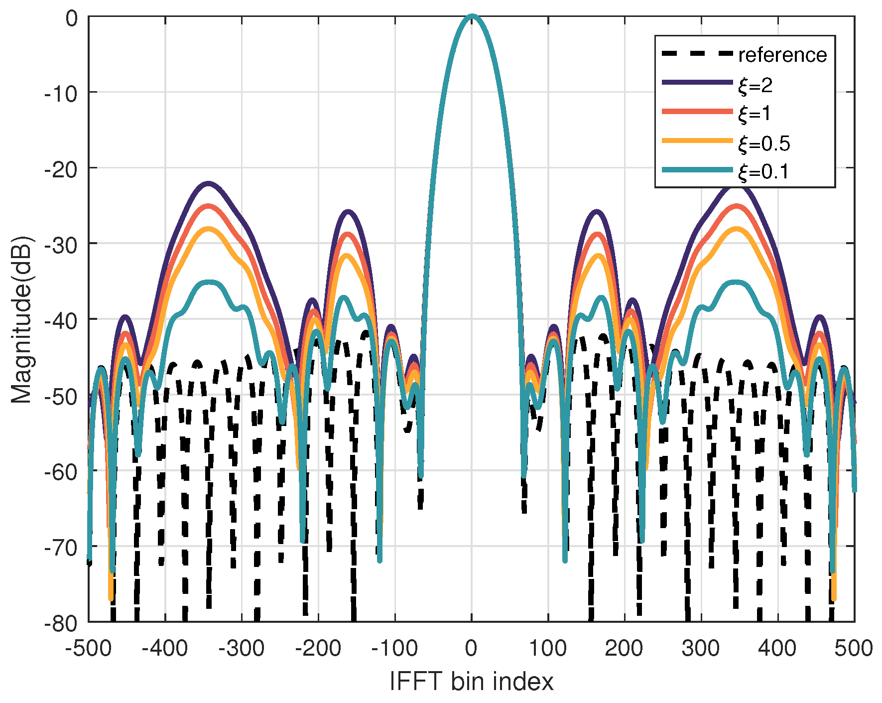
4.1. Receive Beampattern Results

Figure 3 presents the receive beampatterns obtained by the proposed method, the ADMM method, and the MM method. As indicated by the green square in Figure 3, all methods are capable of forming a high-energy main lobe at the target location. Moreover, as observed from the clutter positions marked by black squares and the interference directions marked by red rectangles, all methods are able to achieve nulling at the clutter and interference locations. This demonstrates that all methods have anti-interference ability through the joint design of waveform and filters.

Figure 4 presents the angle profile of the receive beampattern extracted at the range where clutter is present, normalized for clearer visualization. Overall, our method achieves deeper nulls at the clutter locations (black dashed lines) and interference directions (blue dashed lines). The process of maximizing SINR involves enhancing the desired signal energy while suppressing interference and clutter to the greatest extent. Figure 4 shows that our proposed method improves the clutter and interference suppression capability of the radar system by improving SINR, which has practical research significance.

4.2. SINR Performance Evaluation

Figure 5 illustrates the variation curve of SINR with respect to iteration time. The findings demonstrate that the SINR values of all methods exhibited an upward trend as the iterations proceed, ultimately converging to a stable state. As shown in the figure, the proposed method improved the SINR performance by about 0.6 dB compared to the MM-based method and by about 0.7 dB compared to the method under the ADMM framework. This improvement can be attributed to the projection of the problem onto the JCCM-CSMS, which can be solved efficiently without the need for relaxation. This avoids relaxation errors and enables a more rigorous optimization of the problem. However, due to the existence of similarity constraints, the design freedom of the waveform is restricted, and the performance improvement is also limited. In radar systems, improving SINR can increase detection range, improve detection probability, reduce false alarm probability, enhance target parameter estimation, and improve performance in complex environments [48,49]. The specific values of SINR of the three methods are shown in

Table 2. Quantitative analysis of system performance.

Method	SINR		Similarity
	3 Clutter Scattering Points	4 Clutter Scattering Points
Proposed Method	22.85 dB	22.60 dB	1.00
ADMM	22.12 dB	22.05 dB	1.00
MM	22.26 dB	21.96 dB	1.00

.

Figure 6 shows the variation of the optimized SINR performance at the receiver as the input SNR changed. As shown in Figure 6, the SINR for all methods improved as the SNR increased. In addition, in the case of higher and lower SNRs, the SINR difference between the ADMM method and the other two methods further increased. This is because the performance of the ADMM method is greatly affected by the value of the relaxation factor. When the objective function value changes significantly, the selected relaxation factor value will gradually become inappropriate.

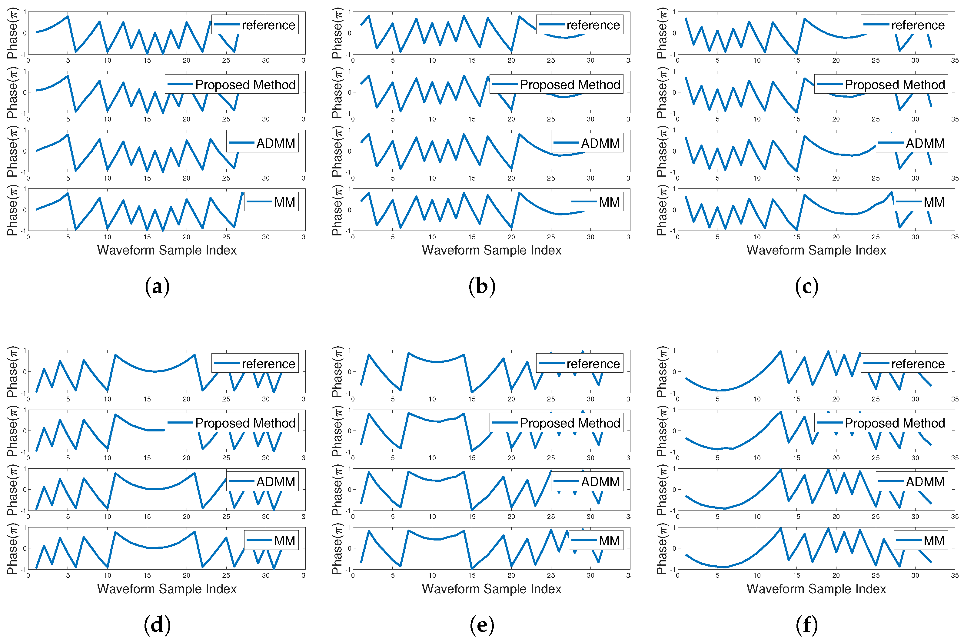
4.3. Analysis of Similarity

Figure 7 illustrates the phase of the transmitted waveforms obtained by the three methods. Since the waveform we designed is of constant modulus, it only contains phase information. Therefore, the similarity to the reference waveform could be assessed based on the phase information. It can be observed that all methods exhibited a high similarity to the reference waveform, thereby satisfying the similarity constraint. The numerical values of similarity are recorded in Table 2.

Figure 8 illustrates the pulse compression diagram of the transmitted waveform obtained by the proposed method. Since the transmitted waveforms of all antennas follow similar principles, we take the transmitted waveform of the first antenna as an example. It can be observed that as the similarity constraint becomes more stringent, the resemblance between the transmitted waveform and the reference waveform grows, thereby endowing the transmitted waveform with even better autocorrelation properties.

4.4. Performance Analysis of a Scenario with More Clutter

In this subsection, we expand the scenario to include four clutter sources, located at $\left(25\mathrm{m},{10}^{\circ }\right)$, $\left(40\mathrm{m},-{10}^{\circ }\right)$, $\left(50\mathrm{m},-{50}^{\circ }\right)$, $\left(60\mathrm{m},{40}^{\circ }\right)$. The clutter power and interference power are set as ${\delta }_{c,q}^2=20\mathrm{dB},\mathrm{q}=1,\cdots ,\mathrm{Q}$ and ${\delta }_{j,k}^2=35\mathrm{dB},\mathrm{k}=1,\cdots ,\mathrm{K}$ respectively. As can be seen from Figure 9, all methods are still capable of forming nulls at the locations of clutter and interference. This demonstrates that the anti-interference performance of all methods exhibits a certain level of robustness across different scenarios, which is essential for practical applications.

Figure 10 illustrates the SINR variation over time under the scenario configured in Section 4.4. As illustrated in the figure, conclusions similar to those in Figure 5 can be drawn, indicating that the proposed method still improves the SINR by approximately 0.6 dB compared with the other two methods. This demonstrates that the proposed method achieves superior SINR performance across different scenarios, exhibiting strong universality. A higher SINR value provides greater advantages in subsequent target detection performance and parameter estimation accuracy [28,29]. The specific values are shown in Table 2.

5. Conclusions

This study investigated the codesign of transmit waveforms and receive filters under similarity constraints in FDA-MIMO systems. The objective is to maximize the SINR while ensuring the efficient operation of power amplifiers without distortion. To address the challenges posed by the non-convex nature of the problem, a method based on JCCM-CSMS is proposed. Simulation results demonstrate that the proposed method achieves a 0.6 dB improvement in SINR compared to existing methods. Additionally, it reduces computational complexity, making it better suited for real-time applications in practical radar systems.

References

1. Chen, G.; Wang, C.; Gong, J.; Xu, J.; Tan, M. Fast and Efficient Single-Snapshot Range and Angle Estimation for FDA-MIMO Radar. IEEE Geosci. Remote. Sens. Lett. 2024, 21, 3509405. [Google Scholar] [CrossRef]
2. Jian, J.; Huang, Q.; Huang, B.; Wang, W.Q. FDA-MIMO-Based Integrated Sensing and Communication System with Frequency Offsets Permutation Index Modulation. IEEE Trans. Commun. 2024, 72, 6707–6721. [Google Scholar] [CrossRef]
3. Wu, M.; Hao, C.; Hu, Q.; Orlando, D. Sparsity-Based Processing to Enhance the Reverberation Suppression for FDA-MIMO Sonars. IEEE Trans. Aerosp. Electron. Syst. 2024, 60, 1556–1569. [Google Scholar] [CrossRef]
4. Gui, R.; Huang, B.; Wang, W.Q.; Sun, Y. Generalized Ambiguity Function for FDA Radar Joint Range, Angle and Doppler Resolution Evaluation. IEEE Geosci. Remote. Sens. Lett. 2022, 19, 3502305. [Google Scholar] [CrossRef]
5. Wu, Z.; Zhu, S.; Xu, J.; Lan, L.; Zhang, M.; Liu, F. Interference Suppression With MR-FDA-MIMO Radar Using Virtual Samples Based Beamforming. IEEE Trans. Aerosp. Electron. Syst. 2024, 60, 5211–5225. [Google Scholar] [CrossRef]
6. Wu, Z.; Zhu, S.; Xu, J.; Lan, L.; Li, X.; Zhang, Y. Frequency Increment Design Method of MR-FDA-MIMO Radar for Interference Suppression. Remote Sens. 2023, 15, 4070. [Google Scholar] [CrossRef]
7. Liu, F.; Zhu, S.; Xu, J.; Li, X.; Lan, L.; Liang, J. Fast Repeater Deception Jamming Suppression With DFI-FDA-MIMO Radar. IEEE Trans. Aerosp. Electron. Syst. 2024, 60, 4271–4284. [Google Scholar] [CrossRef]
8. An, D.; Hu, J.; Zuo, Y.; Zhong, K.; Xiao, X.; Li, H.; Li, L. Robust Transceiver Design for ISAC Systems via Product Complex Circle-Sphere Manifold Method. IEEE Trans. Instrum. Meas. 2024, 73, 5501914. [Google Scholar] [CrossRef]
9. Zhong, K.; Hu, J.; Liu, J.; An, D.; Pan, C.; Teh, K.C.; Yu, X.; Li, H. P2C2M: Parallel Product Complex Circle Manifold for RIS-Aided ISAC Waveform Design. IEEE Trans. Cogn. Commun. Netw. 2024, 10, 1441–1451. [Google Scholar] [CrossRef]
10. Yu, X.; Cui, G.; Kong, L.; Li, J.; Gui, G. Constrained Waveform Design for Colocated MIMO Radar With Uncertain Steering Matrices. IEEE Trans. Aerosp. Electron. Syst. 2019, 55, 356–370. [Google Scholar] [CrossRef]
11. Fan, W.; Liang, J.; Li, J. Constant Modulus MIMO Radar Waveform Design With Minimum Peak Sidelobe Transmit Beampattern. IEEE Trans. Signal Process. 2018, 66, 4207–4222. [Google Scholar] [CrossRef]
12. Wang, S.; Dai, W.; Wang, H.; Li, G.Y. Robust Waveform Design for Integrated Sensing and Communication. IEEE Trans. Signal Process. 2024, 72, 3122–3138. [Google Scholar] [CrossRef]
13. Zhao, Y.; Zhao, Z.; Tong, F.; Sun, P.; Feng, X.; Zhao, Z. Joint Design of Transmitting Waveform and Receiving Filter via Novel Riemannian Idea for DFRC System. Remote Sens. 2023, 15, 3548. [Google Scholar] [CrossRef]
14. Shi, S.; Wang, Z.; He, Z.; Cheng, Z. Constrained waveform design for dual-functional MIMO radar-Communication system. Signal Process. 2020, 171, 107530. [Google Scholar] [CrossRef]
15. Jia, W.; Jakobsson, A.; Wang, W.Q. Designing FDA Radars Robust to Contaminated Shared Spectra. IEEE Trans. Aerosp. Electron. Syst. 2023, 59, 2861–2873. [Google Scholar] [CrossRef]
16. Jia, W.; Jakobsson, A.; Wang, W.Q. Waveform optimization with SINR criteria for FDA radar in the presence of signal-dependent mainlobe interference. Signal Process. 2023, 204, 108851. [Google Scholar] [CrossRef]
17. Du, L.; Zhang, S.; Huang, L.; Wang, W.Q. Joint LPI waveform and passive beamforming design for FDA-MIMO-DFRC systems. Signal Process. 2025, 227, 109727. [Google Scholar] [CrossRef]
18. Ni, Y.; Wang, Z.; Huang, Q. Joint Transceiver Beamforming for Multi-Target Single-User Joint Radar and Communication. IEEE Wirel. Commun. Lett. 2022, 11, 2360–2364. [Google Scholar] [CrossRef]
19. Li, Z.; Shi, J.; Liu, W.; Pan, J.; Li, B. Robust Joint Design of Transmit Waveform and Receive Filter for MIMO-STAP Radar Under Target and Clutter Uncertainties. IEEE Trans. Veh. Technol. 2022, 71, 1156–1171. [Google Scholar] [CrossRef]
20. Lan, L.; Rosamilia, M.; Aubry, A.; De Maio, A.; Liao, G. FDA-MIMO Transmitter and Receiver Optimization. IEEE Trans. Signal Process. 2024, 72, 1576–1589. [Google Scholar] [CrossRef]
21. Gong, P.; Zhang, Z.; Wu, Y.; Wang, W.Q. Joint Design of Transmit Waveform and Receive Beamforming for LPI FDA-MIMO Radar. IEEE Signal Process. Lett. 2022, 29, 1938–1942. [Google Scholar] [CrossRef]
22. Wu, W.; Tang, B.; Wang, X. Constant-Modulus Waveform Design for Dual-Function Radar-Communication Systems in the Presence of Clutter. IEEE Trans. Aerosp. Electron. Syst. 2023, 59, 4005–4017. [Google Scholar] [CrossRef]
23. Wu, L.; Babu, P.; Palomar, D.P. Transmit Waveform/Receive Filter Design for MIMO Radar With Multiple Waveform Constraints. IEEE Trans. Signal Process. 2018, 66, 1526–1540. [Google Scholar] [CrossRef]
24. Zhong, K.; Hu, J.; Cong, Y.; Cui, G.; Hu, H. RMOCG: A Riemannian Manifold Optimization-Based Conjugate Gradient Method for Phase-Only Beamforming Synthesis. IEEE Antennas Wirel. Propag. Lett. 2022, 21, 1625–1629. [Google Scholar] [CrossRef]
25. Yuan, X.; Huang, W.; Absil, P.A.; Gallivan, K. A Riemannian Limited-Memory BFGS Algorithm for Computing the Matrix Geometric Mean. Procedia Comput. Sci. 2016, 80, 2147–2157. [Google Scholar] [CrossRef]
26. Yang, R.; Jiang, H.; Qu, L. Joint Constant-Modulus Waveform and RIS Phase Shift Design for Terahertz Dual-Function MIMO Radar and Communication System. Remote Sens. 2024, 16, 3083. [Google Scholar] [CrossRef]
27. Xu, K.; Sun, G.; Ji, Y.; Ding, Z.; Chen, W. Multiple-Input Multiple-Output Synthetic Aperture Radar Waveform and Filter Design in the Presence of Uncertain Interference Environment. Remote Sens. 2024, 16, 4413. [Google Scholar] [CrossRef]
28. Wang, Y.; Sun, Y.; Wang, J.; Shen, Y. Dynamic Spectrum Tracking of Multiple Targets With Time-Sparse Frequency-Hopping Signals. IEEE Signal Process. Lett. 2024, 31, 1675–1679. [Google Scholar] [CrossRef]
29. Li, Y.; Su, H.; Chen, J.; Wang, W.; Wang, Y.; Duan, C.; Chen, A. A Contrast-Enhanced Approach for Aerial Moving Target Detection Based on Distributed Satellites. Remote Sens. 2025, 17, 880. [Google Scholar] [CrossRef]
30. Zhong, T.; Tao, H.; Cao, H.; Liao, H. Multiparameter Estimation for Monostatic FDA-MIMO Radar With Polarimetric Antenna. IEEE Trans. Antennas Propag. 2024, 72, 2524–2539. [Google Scholar] [CrossRef]
31. Fang, Y.; Zhu, S.; Liao, B.; Li, X.; Liao, G. Target Localization With Bistatic MIMO and FDA-MIMO Dual-Mode Radar. IEEE Trans. Aerosp. Electron. Syst. 2024, 60, 952–964. [Google Scholar] [CrossRef]
32. Ding, Z.; Xie, J.; Lan, L.; Qi, C.; Gao, X. An Intelligent Anti-Interference Scheme for FDA-MIMO Radar Under Nonideal Condition. IEEE Trans. Aerosp. Electron. Syst. 2024, 60, 3269–3281. [Google Scholar] [CrossRef]
33. Li, M.; Wang, W.Q. Performance Analysis of Joint Radar-Communication System Based on FDA-MIMO Radar. IEEE Access 2024, 12, 48774–48787. [Google Scholar] [CrossRef]
34. Xie, Q.; Wang, Z.; Wen, F.; He, J.; Truong, T.K. Coarray Tensor Train Decomposition for Bistatic MIMO Radar with Uniform Planar Array. IEEE Trans. Antennas Propag. 2025, early access, 1. [Google Scholar] [CrossRef]
35. Shao, S.; Wang, W.Q.; Sun, Y.; Zhang, S. Effects of Spatial Position on Mainlobe Interference Suppression Performance of FDA-MIMO Radar. IEEE Trans. Aerosp. Electron. Syst. 2024, 60, 9437–9443. [Google Scholar] [CrossRef]
36. Xiao, M.; Hu, T.; Shao, X.; Wu, L.; Xiao, Z. A Single-Snapshot Robust Beamforming for FDA-MIMO Radar Based on AID3. IEEE Trans. Veh. Technol. 2025, 74, 38–49. [Google Scholar] [CrossRef]
37. Wu, Z.; Zhu, S.; Xu, J.; Lan, L.; Li, X.; Zhang, Z. Analysis of interference suppression performance in MR-FDA-MIMO radar. Signal Process. 2025, 230, 109873. [Google Scholar] [CrossRef]
38. Miao, L.; Zhang, S.; Huang, L.; Ding, J.; Wang, W.Q. Moving Target Detection Using FDA-MIMO Radar With Planar Array. IEEE Geosci. Remote. Sens. Lett. 2024, 21, 1–5. [Google Scholar] [CrossRef]
39. Zhong, K.; Hu, J.; Li, H.; Wang, Y.; Cheng, X.; Cheng, X.; Pan, C.; Teh, K.C.; Cui, G. Joint Design of Power Allocation and Unimodular Waveform for Polarimetric Radar. IEEE Trans. Geosci. Remote. Sens. 2025, 63, 5100612. [Google Scholar] [CrossRef]
40. Tsinos, C.G.; Arora, A.; Chatzinotas, S.; Ottersten, B. Joint Transmit Waveform and Receive Filter Design for Dual-Function Radar-Communication Systems. IEEE J. Sel. Top. Signal Process. 2021, 15, 1378–1392. [Google Scholar] [CrossRef]
41. Sha, Y.; Feng, X.; Wei, T.; Du, J.; Yu, W. Anti-Maneuvering Repeater Jamming Using Up- and Down-Chirp Modulation in Spaceborne Synthetic Aperture Radar. Remote Sens. 2024, 16, 4260. [Google Scholar] [CrossRef]
42. Mao, X.; Cai, B.; Xia, M.; Yang, L. Research on Optimization Design Method of MIMO Radar Waveform Based on Frequency-Orthogonal LFM. IEEE Access 2024, 12, 160835–160845. [Google Scholar] [CrossRef]
43. Wang, P.; Wang, Z.; You, P.; An, M. Algorithm for Designing Waveforms Similar to Linear Frequency Modulation Using Polyphase-Coded Frequency Modulation. Remote Sens. 2024, 16, 3664. [Google Scholar] [CrossRef]
44. Zhong, K.; Hu, J.; Pan, C.; Deng, M.; Fang, J. Joint Waveform and Beamforming Design for RIS-Aided ISAC Systems. IEEE Signal Process. Lett. 2023, 30, 165–169. [Google Scholar] [CrossRef]
45. Zhong, K.; Hu, J.; Zhao, Z.; Yu, X.; Cui, G.; Liao, B.; Hu, H. MIMO Radar Unimodular Waveform Design With Learned Complex Circle Manifold Network. IEEE Trans. Aerosp. Electron. Syst. 2024, 60, 1798–1807. [Google Scholar] [CrossRef]
46. Zhong, K.; Hu, J.; Li, H.; Wang, R.; An, D.; Zhu, G.; Teh, K.C.; Pan, C.; Eldar, Y.C. RIS-Aided Beamforming Design for MIMO Systems via Unified Manifold Optimization. IEEE Trans. Veh. Technol. 2025, 74, 674–685. [Google Scholar] [CrossRef]
47. Ring, W.; Wirth, B. Optimization Methods on Riemannian Manifolds and Their Application to Shape Space. SIAM J. Optim. 2012, 22, 596–627. [Google Scholar] [CrossRef]
48. Zhang, H.; Liu, W.; Zhang, Q.; Zhang, L.; Liu, B.; Xu, H.X. Joint Power, Bandwidth, and Subchannel Allocation in a UAV-Assisted DFRC Network. IEEE Internet Things J. 2025, 12, 11633–11651. [Google Scholar] [CrossRef]
49. Zhang, H.; Liu, W.; Zhang, Q.; Liu, B. Joint Customer Assignment, Power Allocation, and Subchannel Allocation in a UAV-Based Joint Radar and Communication Network. IEEE Internet Things J. 2024, 11, 29643–29660. [Google Scholar] [CrossRef]
Figure 1. The structure of the frequency diverse array–multiple input multiple output (FDA-MIMO) radar.
Remotesensing 17 01800 g001
Figure 2. Schematic diagram of joint complex circle manifold–complex sphere manifold space (JCCM-CSMS).
Remotesensing 17 01800 g002
Figure 3. Range-angle domain receive beampattern: (a) the proposed method, (b) ADMM, and (c) MM. The target position is marked by a green square, the clutter positions are marked by black squares, and the interference directions are marked by red rectangles.
Remotesensing 17 01800 g003
Figure 4. Angle profile of the receive Beampattern: (a) angle profile at a distance of 25 m, (b) angle profile at a distance of 50 m, and (c) angle profile at a distance of 70 m.
Remotesensing 17 01800 g004
Figure 5. Correlation between Signal to Interference plus Noise Ratio (SINR) and iteration time.
Remotesensing 17 01800 g005
Figure 6. Output SINR versus transmit Signal-to-noise Ratio (SNR).
Remotesensing 17 01800 g006
Figure 7. The phase of the transmitted waveform. (a) The 1st transmit antenna. (b) The 2nd transmit antenna. (c) The 3rd transmit antenna. (d) The 4th transmit antenna. (e) The 5th transmit antenna. (f) The 6th transmit antenna.
Remotesensing 17 01800 g007
Figure 8. Pulse compression diagram of the transmitted waveform.
Remotesensing 17 01800 g008
Figure 9. Range-angle domain receive beampattern: (a) the proposed method, (b) ADMM, and (c) MM. The target position is marked by a green square, the clutter positions are marked by black squares, and the interference directions are marked by red rectangles.
Remotesensing 17 01800 g009
Figure 10. Correlation between SINR and iteration time.
Remotesensing 17 01800 g010