A New Quasi-Linear Integral Transform Between Ocean Wave Spectrum and Phase Spectrum of an XTI-SAR

Abstract

Cross-Track Interferometric Synthetic Aperture Radar (XTI-SAR) can utilize variations in interferometric phase to measure sea surface velocity along radar radial direction and sea surface height, which can be used for ocean wave parameter inversion. However, research on the imaging mechanisms of XTI-SAR systems for ocean waves remains understudied, and there are still some problems in its perception. To further study the imaging mechanism of XTI-SAR measurement systems for ocean waves, this paper describes research based on the nonlinear integral transform model and the quasi-linear integral transform model derived by Bao in 1999, which relate the XTI-SAR ocean wave spectrum to the phase spectrum. Firstly, this work derived another quasi-linear integral transform model based on the nonlinear integral transform model, and also optimized the quasi-linear integral transform model derived by Bao. The optimized quasi-linear integral transform model eliminates the need for complex calculations of cross-correlation functions between sea surface height and radar radial orbital velocity components of ocean waves, as well as the radar line-of-sight velocity transfer function, while maintaining high integral transform accuracy. Secondly, based on two-dimensional sea surface simulations, we analyzed the differences between the quasi-linear integral transform models and the nonlinear integral transform model corresponding to different XTI-SAR system configurations and different sea states. The numerical simulation results show that, for the XTI-SAR system, in general, the difference between the quasi-linear integral transform model derived in this work and the nonlinear integral transform model is greater than that of the quasi-linear integral transform model derived by Bao. However, the difference between the optimized quasi-linear integral transform model and the nonlinear integral transform model in this study is smaller, and it is more convenient when transforming the ocean wave spectrum to the phase spectrum.

1. Introduction

As one of the critical marine dynamic environmental elements, the precise observation of ocean waves significantly enhances marine environmental forecasting capabilities, and plays a crucial role in maritime disaster mitigation and prevention. Consequently, ocean wave studies hold substantial scientific significance [1,2,3]. Ocean remote sensing, capable of acquiring global-scale ocean wave parameters, effectively compensates for the spatial limitations inherent in in situ buoy measurements, and has consequently emerged as a focal research area in marine remote sensing studies [4,5,6].

Interferometric Synthetic Aperture Radar (InSAR) acquires ocean wave parameters by processing the interferometric phase, which is generated from a pair of registered master and slave SAR images of the same sea area obtained simultaneously using dual antennas [7]. Based on the spatial relationship between the baseline formed by the dual antennas and the platform flight direction. InSAR systems are primarily categorized into Along-Track InSAR (ATI-SAR) and Cross-Track InSAR (XTI-SAR). ATI-SAR refers to an InSAR measurement mode where the baseline between antennas is parallel to the platform flight direction [8]. Since the slant range difference between the master/slave antennas and sea surface targets is closely related to the motion state of scattering targets, the along-track interferometric phase can be utilized for measuring sea surface target motion parameters. XTI-SAR, which is the focus of this study, refers to an InSAR measurement configuration where the baseline formed by the dual antennas is perpendicular to the platform flight direction [9]. Since the slant range difference between the master/slave antennas and sea surface targets exhibits a close relationship with sea surface height, XTI-SAR enables sea surface height measurements through the analysis of cross-track interferometric phases [10].

Compared to a traditional SAR system, the dual-antenna XTI-SAR measurement system demonstrates superior capabilities in ocean wave monitoring. Firstly, the interferometric phase acquired from XTI-SAR master/slave image pairs exhibits direct proportionality to sea surface height. This intrinsic proportionality enables the direct inversion of sea surface height through XTI-SAR ocean wave remote sensing, bypassing complex inversion algorithms required by traditional SAR systems [11,12]. Secondly, since the XTI-SAR interferometric phase image is almost unaffected by the Real Aperture Radar (RAR) modulation transfer function (MTF), the XTI-SAR measurement system is more suitable than traditional SAR systems for acquiring two-dimensional ocean wave direction spectra [13,14].

To investigate the imaging principles of XTI-SAR for ocean waves, Bao established a nonlinear integral transform model and a quasi-linear integral transform model between the ocean wave spectrum and the phase spectrum in 1999 [15]. This model was derived from the function relationship between the sea surface interferometric phase measured by XTI-SAR and sea surface height, incorporating both the sea surface height term and the sea surface orbital velocity term to transform two-dimensional ocean wave spectra into corresponding phase spectra. However, this integral transform model, which is relatively complex and poses challenges in comprehending the influence of velocity bunching on XTI-SAR ocean wave imaging mechanisms, omits the derivative term of the ocean wave orbital velocity along the radar radial direction. Moreover, although the quasi-linear integral transform between ocean wave spectrum and phase spectrum derived by Bao facilitates the interpretation of velocity bunching effects on XTI-SAR ocean wave imaging compared to nonlinear integral transform, the computational process remains intricate and computationally intensive. In 2001, Schulz-Stellenfleth et al. developed an ocean wave imaging model for XTI-SAR measurement system based on backscattered echo signals from the sea surface [16]. Additionally, they numerically simulated corresponding phase spectra and SAR intensity image spectra from given two-dimensional ocean wave spectra. By simultaneously employing Monte Carlo methods integrated with forward integral transform relationships, the team simulated two-dimensional variance spectra incorporating a distorted Digital Elevation Model (DEM). The research results show that, for small-amplitude swells, when using a distorted DEM to calculate wave heights, the calculated wave height error is less than 10%. However, this error is related to the sea surface correlation time and the actual propagation direction of the ocean waves. For small-scale wind waves propagating along the image azimuth direction, the calculated wave heights by Schulz-Stellenfleth et al. were significantly lower than the true values. In the same year, Schulz-Stellenfleth et al. conducted an X-band, horizontally polarized airborne XTI-SAR experiment in the North Sea, and calculated a bunching DEM based on the wave phase data obtained from the experiment [17]. Research findings demonstrate that, when nonlinear effects are weak during XTI-SAR ocean wave imaging, the one-dimensional wave spectra and significant wave heights (SWH) calculated by Schulz-Stellenfleth et al. are basically consistent with the buoy measurement results. However, a systematic discrepancy of approximately 30° persists between their computed dominant ocean wave propagation directions and in situ buoy measurements. In 2007, Zhang et al. developed an interferometric phase model for the XTI-SAR measurement system for large-scale swells and derived the corresponding analytical expression, which takes into account the velocity bunching effect and the influence of sea surface height [18]. Meanwhile, Zhang et al. also studied the imaging mechanism of swells propagating along the azimuth direction in the XTI-SAR measurement system, and derived the corresponding analytical expression. The research shows that the degree of nonlinearity in ocean wave imaging of the XTI-SAR measurement system depends on the radar configuration parameters and sea state conditions, and they believe that the nonlinearity degree of the ocean wave imaging of the XTI-SAR system depends on the radar configurations as well as the sea state.

In 2010, addressing observational challenges of submesoscale ocean dynamics phenomena, National Aeronautics and Space Administration (NASA) proposed the Surface Water and Ocean Topography (SWOT) altimetry satellite mission [19,20]. Equipping with a Ka-band radar interferometer, SWOT achieves unprecedented altimetric accuracy of 1–2 cm@5 × 5 km², enabling high-precision measurements of marine dynamic parameters. This capability effectively addresses the limitations of traditional radar altimeters in observing mesoscale and sub-mesoscale ocean dynamic environmental parameters [21,22]. In 2016, focusing on the scientific issues of ocean sub-mesoscale and sea surface wave phenomena, Chen et al. conducted research on a wide-swath interferometric radar altimeter with a small incidence angle [23]. In 2020–2022, Yang et al. retrieved ocean wave spectra from airborne low incidence angle XTI-SAR images, which demonstrated the feasibility of airborne low incidence XTI-SAR measurements of ocean waves [24,25,26,27]. Unfortunately, Yang et al. did not discuss in detail the effects of random phase noise and velocity bunching effect on the ocean wave inversion based on the airborne low incidence XTI-SAR images, which are important factors affecting the accuracy of ocean wave inversion. In response to this, Sun et al. analyzed and discussed the above two factors in detail when performing ocean wave inversion based on XTI-SAR images [28,29].

Due to sea surface motion, the sea surface scattering facet will shift along the azimuth direction during the mapping process to the XTI-SAR image, causing the XTI-SAR system to image ocean waves as a nonlinear process [30,31,32]. Since the XTI-SAR interferometric phase is closely related to sea surface height, studying the integral transform between the XTI-SAR phase spectrum and the ocean wave spectrum can provide a better understanding of the imaging mechanism of the XTI-SAR system for ocean waves. The nonlinear integral transform between the XTI-SAR ocean wave spectrum and phase spectrum derived by Bao exhibits significant complexity, which makes it challenging to comprehensively elucidate the influence of velocity bunching on XTI-SAR ocean wave imaging mechanisms. Furthermore, the quasi-linear integral transform derived from the nonlinear framework still involves intricate calculations and high computational workloads. Therefore, to better understand the XTI-SAR ocean wave imaging mechanisms and the role of velocity bunching in the XTI-SAR ocean wave imaging mechanism, this study will further carry out the study on quasi-linear integral transform between ocean wave spectrum and phase spectrum, aiming to simplify the computational procedures of existing quasi-linear integral transform model and reduce associated computational workloads.

The content structure of this paper is organized as follows. Section 2 introduces the existing nonlinear and quasi-linear integral transform models derived by Bao between the phase spectrum and the ocean wave spectrum, a new quasi-linear integral transform model derived in this paper, and the optimization of the existing quasi-linear integral transform model derived by Bao. Section 3 provides a detailed analysis of the differences between the quasi-linear integral transform models and the nonlinear integral transform model. Conclusions and a summary are given in Section 4.

2. Methods

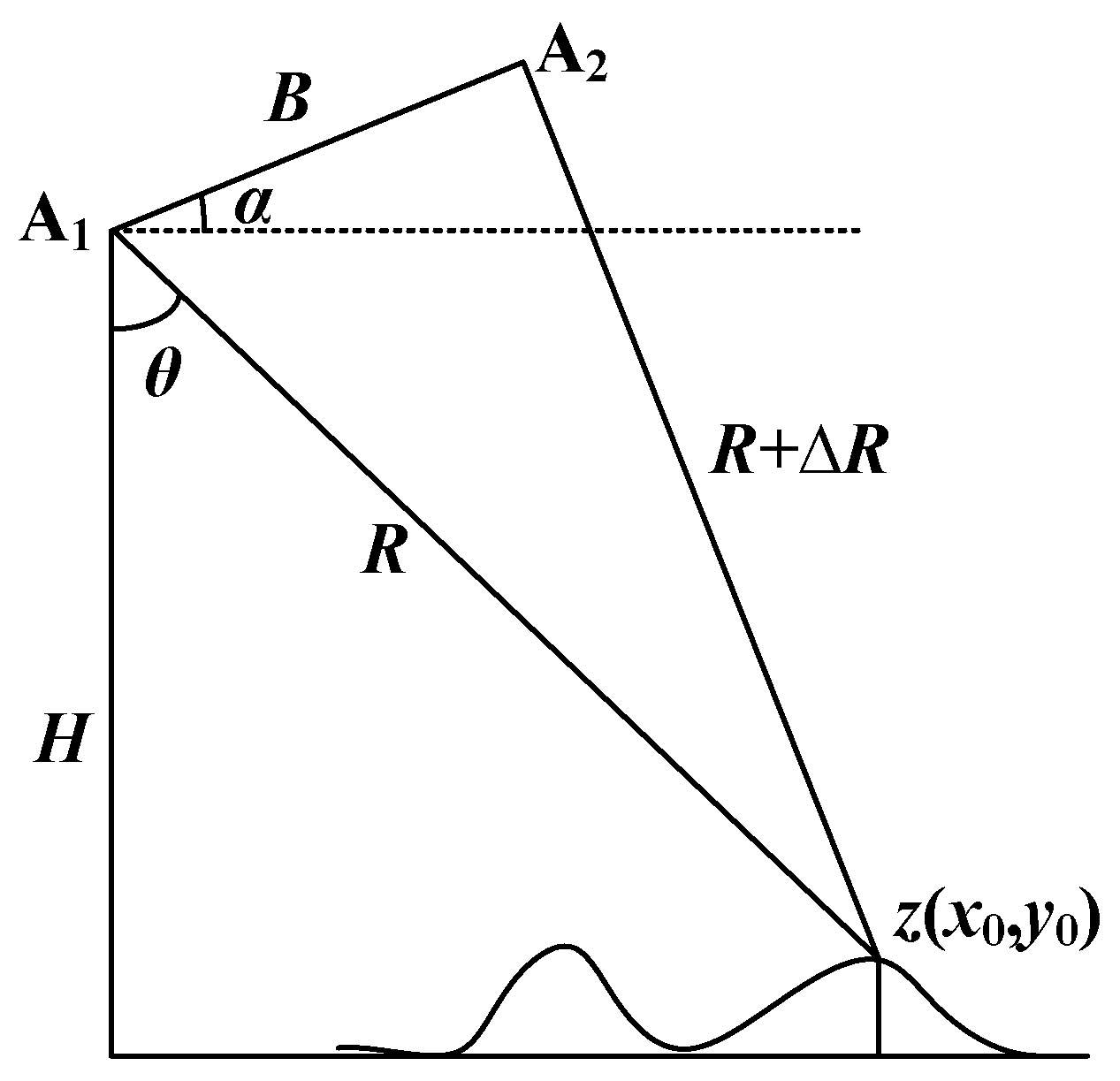
2.1. The Nonlinear Integral Transform Model

Figure 1 illustrates the geometric schematic diagram of height measurement for the XTI-SAR system. The altimetry phase difference for height measurement is determined by the slant range difference between the two antennas and the target in XTI-SAR systems, which is related to the elevation of the ground scattering facet. The phase difference (∆φ) between the two antennas can be expressed as

$$\Delta \phi ={\displaystyle \frac{4\pi }{{\lambda }_i}}\Delta R$$

(1)

where λ_i represents the wavelength of the incidence electromagnetic wave, and ∆R is the slant range difference between the two antennas and the target. As can be seen from Figure 1, the two antennas and the sea surface target form a triangle, and we can derive Equation (2) based on the cosine theorem.

$${\left(R+\Delta R\right)}^2=R^2+B^2+2RB\sin \left(\theta -\alpha \right)$$

(2)

Since the slant range R between the antenna and the target is much larger than the baseline length B and the slant range difference ∆R, the terms B² and ∆R² in the expansion of Equation (2) can be neglected, and we can derive that

$$\Delta R=B\sin \left(\theta -\alpha \right)$$

(3)

where θ denotes the incidence angle of the electromagnetic wave, and α the baseline roll angle. When measuring ocean waves using the XTI-SAR system, the interference fringes in the interferogram calculated from the XTI-SAR master and slave images are primarily caused by the flat-earth phase [28]. This flat-earth phase not only contributes nothing to the sea surface height but also interferes with subsequent wave inversion. Therefore, the influence of the flat-earth phase must be removed prior to wave inversion. Methods for removing the flat-earth phase can be referenced in [28]. After removing the flat-earth phase, the sea surface height phase can be expressed as Equation (4):

$${\phi }_{SSH}=-{\displaystyle \frac{4\pi B\cos \left(\theta -\alpha \right)}{{\lambda }_{i}R\sin \theta }}z\left(x_0\right)$$

(4)

where z(x₀) represents the sea surface height at the position x₀ = (x₀, y₀) on the sea surface. x₀ is the azimuth direction, and y₀ the range direction. If a scattering element on the sea surface has a radial velocity component u_r(x₀), this scattering element will exhibit an azimuth shift in the XTI-SAR phase image, and the shift magnitude is given by Equation (5):

$$\Delta az={\displaystyle \frac{R}{V}}{u}_r\left(x_0\right)$$

(5)

where V denotes the velocity of the platform carrying the XTI-SAR. If both the shift and the ground range pulse response function can be approximated using the delta function (δ), then Equation (4) can be re-expressed as Equation (6) [15].

$${\phi }_{SSH}\left(x\right)=-{\displaystyle \frac{4\pi B\cos \left(\theta -\alpha \right)}{{\lambda }_{i}R\sin \theta }}{\displaystyle \int z\left(x_0\right)\delta \left(y-y_0\right)\delta \left[x-x_0-\frac{R}{V}{u}_r\left(x_0\right)\right]}d{x}_0$$

(6)

Based on Equation (6), Bao derived a nonlinear integral transform using the characteristic function method to convert the ocean wave spectrum into the XTI-SAR phase spectrum P(k) [33,34,35], which is shown in Equation (7):

$$\begin{array}{c}P\left(k\right)={\left[{\displaystyle \frac{B\cos \left({\theta }_0-\alpha \right)}{2\pi \lambda R\sin \left({\theta }_0\right)}}\right]}^2{\displaystyle \int \exp \left[\frac{k_x^2{R}^2}{V^2}\left(f^u\left(r\right)-f^u\left(0\right)\right)\right]}\\ \hspace{1em}\hspace{1em}\hspace{1em}\hspace{1em}\hspace{1em}\hspace{1em}\hspace{1em}\hspace{1em}\hspace{1em}\hspace{1em}\left\{f^h\left(r\right)+{\displaystyle \frac{k_x^2{R}^2}{V^2}}\left[f^{hu}\left(r\right)-f^{hu}\left(0\right)\right]\left[f^{hu}\left(-r\right)-f^{hu}\left(0\right)\right]\right\}\exp \left(-jkr\right)dr\end{array}$$

(7)

where r denotes spatial offset, k(k_x,k_y) represents the two-dimensional wavenumber, k_x and k_y represent the azimuth and range wavenumber component, respectively. f^h(r) represents the autocorrelation function of the sea surface height z(x₀), f^u(r) represents the autocorrelation function of the radial orbital velocity component of the ocean waves u_r(x₀), f^hu(r) represents the cross-correlation function between the sea surface height and the radial orbital velocity component, and the three correlation functions can be expressed as Equations (8)–(10), respectively,

$$\begin{array}{c}{f}^h\left(r\right)=〈z\left(x_0\right)z\left(x_0+r\right)〉\hfill \\ \hfill \hspace{1em}\hspace{1em}\hspace{0.17em}={\left(2\pi \right)}^{-2}{\displaystyle \int \exp \left(jkr\right)\left\{\frac{1}{2}\left[S\left(k\right)+S\left(-k\right)\right]\right\}}dk\end{array}$$

(8)

$$\begin{array}{c}{f}^u\left(r\right)=〈u_r\left(x_0\right)u_r\left(x_0+r\right)〉\hfill \\ \hfill \hspace{1em}\hspace{1em}\hspace{0.17em}={\left(2\pi \right)}^{-2}{\displaystyle \int \exp \left(jkr\right)\left\{\frac{1}{2}\left[{\left|T_k^v\left(k\right)\right|}^{2}S\left(k\right)+{\left|T_k^v\left(-k\right)\right|}^{2}S\left(-k\right)\right]\right\}}dk\end{array}$$

(9)

$$\begin{array}{c}{f}^{hu}\left(r\right)=〈u_r\left(x_0\right)z\left(x_0+r\right)〉\hfill \\ \hfill \hspace{1em}\hspace{1em}\hspace{0.17em}\hspace{0.17em}={\left(2\pi \right)}^{-2}{\displaystyle \int \exp \left(jkr\right)\left\{\frac{1}{2}\left[T_k^{v*}\left(k\right)S\left(k\right)+T_k^{v*}\left(-k\right)S\left(-k\right)\right]\right\}}dk\end{array}$$

(10)

where S(k) and S(−k) denote the ocean wave spectra, $T_k^v\left(k\right)$ represents the line-of-sight (LOS) velocity transfer function [36], and $T_k^{v*}\left(k\right)$ is the complex conjugate of $T_k^v\left(k\right)$,

$$T_k^v\left(k\right)=-\omega \left[\sin \theta {\displaystyle \frac{k_y}{\left|k\right|}}+i\cos \theta \right]$$

(11)

with

$$\omega =\sqrt{gk}$$

(12)

where g is the gravitational acceleration constant, and i = (−1)^0.5 represents the imaginary unit. In addition, it can be found from Equation (7) that the exponential term of $-\exp \left[\left(k_x^2{R}^2/V^2\right)f^u\left(0\right)\right]$ is a constant term, which can be seen from Equation (13). Depending on whether this constant term is included in the Taylor series expansion, two different quasi-linear integral transform models between phase spectrum and ocean wave spectrum can be derived, and the exponential terms are shown in Equations (13) and (14), respectively.

$$\begin{array}{c}{f}_1\left(r\right)=\exp \left\{{\displaystyle \frac{k_x^2{R}^2}{V^2}}\left[f^u\left(r\right)-f^u\left(0\right)\right]\right\}\hfill \\ \hfill \hspace{1em} =-\exp \left[{\displaystyle \frac{k_x^2{R}^2}{V^2}}{f}^u\left(0\right)\right]\exp \left[{\displaystyle \frac{k_x^2{R}^2}{V^2}}{f}^u\left(r\right)\right]\end{array}$$

(13)

$$f_2\left(r\right)=\exp \left[{\displaystyle \frac{k_x^2{R}^2}{V^2}}{f}^u\left(r\right)\right]$$

(14)

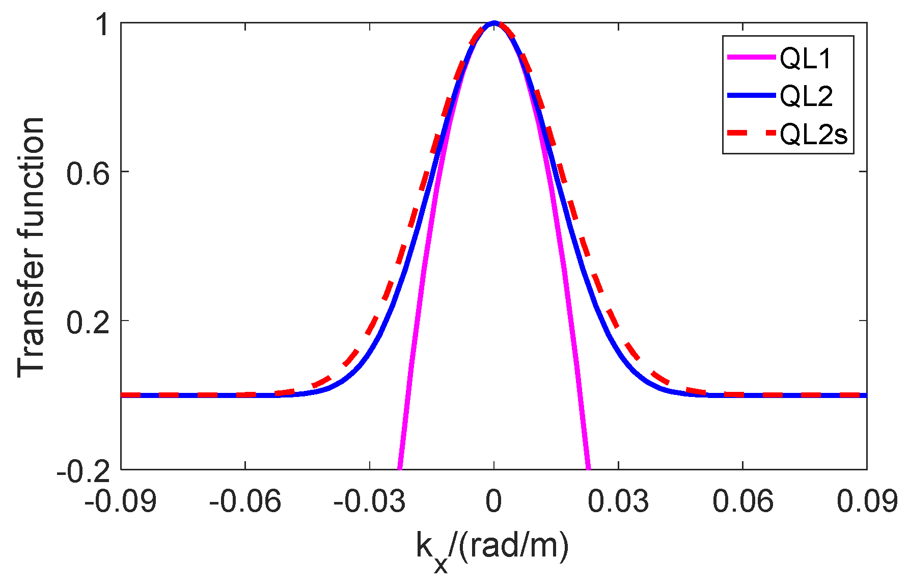
2.2. The First Quasi-Linear Integral Transform Model (QL1)

The first quasi-linear integral transform model between the XTI-SAR phase spectrum and the ocean wave spectrum introduced in this paper is derived by performing a Taylor series expansion on the exponential term in Equation (13). First, expanding the exponential term in Equation (13) via a Taylor series yields

$$\begin{array}{c}\exp \left\{{\displaystyle \frac{k_x^2{R}^2}{V^2}}\left[f^u\left(r\right)-f^u\left(0\right)\right]\right\}=1+{\displaystyle \frac{k_x^2{R}^2}{V^2}}\left[f^u\left(r\right)-f^u\left(0\right)\right]\hfill \\ \hfill \hspace{1em}\hspace{1em}\hspace{1em}\hspace{1em}\hspace{1em}\hspace{1em}\hspace{1em}\hspace{1em}\hspace{1em}\hspace{1em}\hspace{1em}+{\displaystyle \frac{k_x^4{R}^4}{2V^4}}{\left[f^u\left(r\right)-f^u\left(0\right)\right]}^2+\cdot \cdot \cdot \end{array}$$

(15)

Then, substituting Equation (15) into Equation (7), and neglecting terms higher than first-order in f^u(r) and f^u(0), we can derive Equation (16).

$$P^{ql1}\left(k\right)=H_k^{X1}{\displaystyle \frac{S\left(k\right)}{2}}+H_{-k}^{X1}{\displaystyle \frac{S\left(-k\right)}{2}}$$

(16)

where $H_k^{X1}$ represents the MTF for the first quasi-linear integral transform between the XTI-SAR phase spectrum and the ocean wave spectrum. It can be expressed as

$$\left\{\begin{array}{l}{H}_k^{X1}={\left[{\displaystyle \frac{B\cos \left(\theta -\alpha \right)}{2\pi \lambda R\sin \left(\theta \right)}}\right]}^2\left\{1-{\displaystyle \frac{k_x^2{R}^2}{V^2}}{f}^u\left(0\right)-{\displaystyle \frac{k_x^2{R}^2}{V^2}}{f}^{hu}\left(0\right)\left[T_k^{u\ast }\left(k\right)+T_k^u\left(k\right)\right]\right\}\\ H_{-k}^{X1}={\left[{\displaystyle \frac{B\cos \left(\theta -\alpha \right)}{2\pi \lambda R\sin \left(\theta \right)}}\right]}^2\left\{1-{\displaystyle \frac{k_x^2{R}^2}{V^2}}{f}^u\left(0\right)-{\displaystyle \frac{k_x^2{R}^2}{V^2}}{f}^{hu}\left(0\right)\left[T_k^{u\ast }\left(-k\right)+T_k^u\left(-k\right)\right]\right\}\end{array}\right.$$

(17)

2.3. The Second Quasi-Linear Integral Transform Model (QL2)

The second quasi-linear integral transform model between the XTI-SAR phase spectrum and the ocean wave spectrum introduced in this paper is derived by Bao in 1999 by performing a Taylor series expansion on the exponential term in Equation (14), which yields

$$\exp \left\{{\displaystyle \frac{k_x^2{R}^2}{V^2}}{f}^u\left(r\right)\right\}=1+{\displaystyle \frac{k_x^2{R}^2}{V^2}}{f}^u\left(r\right)+{\displaystyle \frac{k_x^4{R}^4}{2V^4}}{\left[f^u\left(r\right)\right]}^2+\cdot \cdot \cdot$$

(18)

Then, substituting Equation (18) into Equation (7), and neglecting terms higher than first-order in f^u(r) and f^u(0), we can derive Equation (19):

$$P^{ql2}\left(k\right)=H_k^{X2}{\displaystyle \frac{S\left(k\right)}{2}}+H_{-k}^{X2}{\displaystyle \frac{S\left(-k\right)}{2}}$$

(19)

where $H_k^{X2}$ represents the MTF for the second quasi-linear integral transform between the XTI-SAR phase spectrum and the ocean wave spectrum. It can be expressed as

$$\left\{\begin{array}{l}{H}_k^{X2}={\left[{\displaystyle \frac{B\cos \left(\theta -\alpha \right)}{2\pi \lambda R\sin \left(\theta \right)}}\right]}^2\exp \left[-{\displaystyle \frac{k_x^2{R}^2}{V^2}}{f}^u\left(0\right)\right]\left\{1-{\displaystyle \frac{k_x^2{R}^2}{V^2}}{f}^{hu}\left(0\right)\left[T_k^{u\ast }\left(k\right)+T_k^u\left(k\right)\right]\right\}\\ H_{-k}^{X2}={\left[{\displaystyle \frac{B\cos \left(\theta -\alpha \right)}{2\pi \lambda R\sin \left(\theta \right)}}\right]}^2\exp \left[-{\displaystyle \frac{k_x^2{R}^2}{V^2}}{f}^u\left(0\right)\right]\left\{1-{\displaystyle \frac{k_x^2{R}^2}{V^2}}{f}^{hu}\left(0\right)\left[T_k^{u\ast }\left(-k\right)+T_k^u\left(-k\right)\right]\right\}\end{array}\right.$$

(20)

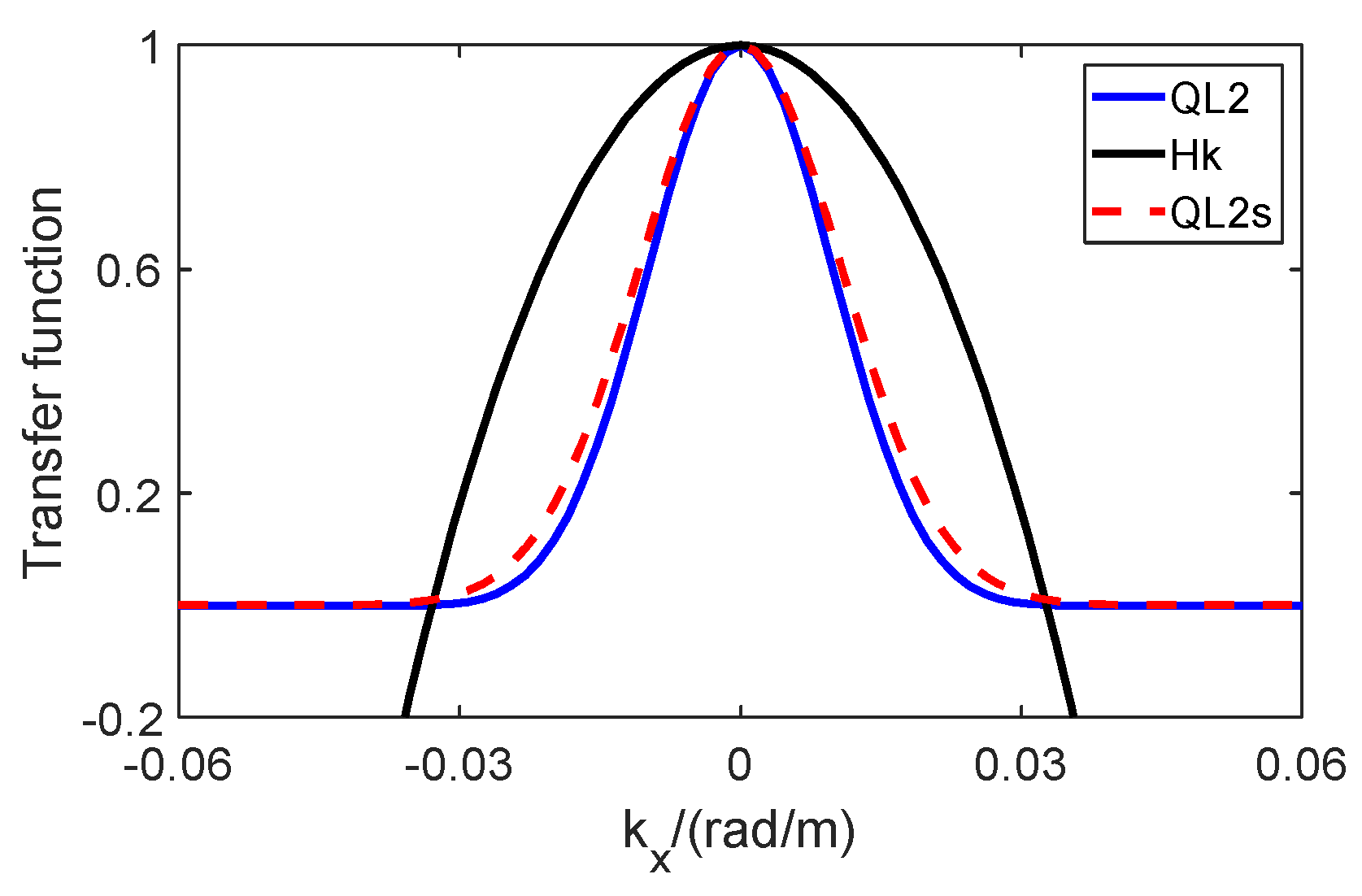
2.4. Optimization of the Second Quasi-Linear Integral Transform Model (QL2s)

Azimuth velocity bunching is one of the important factors affecting XTI-SAR and SAR azimuth ocean wave imaging, and it is also the main research object of Bao in deriving the integral transform model between ocean wave spectrum and phase spectrum. For traditional spaceborne SAR imaging systems with medium incidence angles, the variation in incidence angle and slant range within an entire SAR image is relatively small. As a result, the first term on the right-hand side of Equations (17) and (20) can be approximated as a constant. Therefore, in subsequent analyses, we neglect the influence of this term by setting it to 1 in this study. In addition, we assume that Equation (21) holds.

$$\left\{\begin{array}{l}{H}_k=1-{\displaystyle \frac{k_x^2{R}^2}{V^2}}{f}^{hu}\left(0\right)\left[T_k^{u\ast }\left(k\right)+T_k^u\left(k\right)\right]\\ H_{-k}=1-{\displaystyle \frac{k_x^2{R}^2}{V^2}}{f}^{hu}\left(0\right)\left[T_k^{u\ast }\left(-k\right)+T_k^u\left(-k\right)\right]\end{array}\right.$$

(21)

Then, Equations (20) and (19) can be approximately expressed as Equations (22) and (23).

$$\left\{\begin{array}{l}{H}_k^{X{2}^{\prime }}=\exp \left[-{\displaystyle \frac{k_x^2{R}^2}{V^2}}{f}^u\left(0\right)\right]H_k\\ H_{-k}^{X{2}^{\prime }}=\exp \left[-{\displaystyle \frac{k_x^2{R}^2}{V^2}}{f}^u\left(0\right)\right]H_{-k}\end{array}\right.$$

(22)

$$P^{ql{2}^{\prime }}\left(k\right)=H_k^{X{2}^{\prime }}{\displaystyle \frac{S\left(k\right)}{2}}+H_{-k}^{X{2}^{\prime }}{\displaystyle \frac{S\left(-k\right)}{2}}$$

(23)

To investigate the azimuth variations of $\exp \left[-\left(k_x^2{R}^2/V^2\right)f^u\left(0\right)\right]$ and $H_k$/$H_{-k}$, we plotted Figure 2. It can be found from 2 that the difference between $\exp \left[-\left(k_x^2{R}^2/V^2\right)f^u\left(0\right)\right]$ and $H_k^{X{2}^{\prime }}$/$H_{-k}^{X{2}^{\prime }}$ is small, coupled with the significant discrepancy between $H_k^{X{2}^{\prime }}$/$H_{-k}^{X{2}^{\prime }}$ and $H_k$/$H_{-k}$. This indicates that, for the second quasi-linear integral transform between the XTI-SAR phase spectrum and the ocean wave spectrum, the azimuth cutoff is predominantly contributed by $\exp \left[-\left(k_x^2{R}^2/V^2\right)f^u\left(0\right)\right]$, while the contribution of $H_k$/$H_{-k}$ is very small, and the difference between $\exp \left[-\left(k_x^2{R}^2/V^2\right)f^u\left(0\right)\right]$ and $H_k^{X{2}^{\prime }}$/$H_{-k}^{X{2}^{\prime }}$ can be considered negligible. Based on this, we neglected the influence of $H_k$ and $H_{-k}$ in Equation (22) and optimized Equation (23) to Equation (24).

$$P^{ql2s}\left(k\right)=\exp \left[-{\displaystyle \frac{k_x^2{R}^2}{V^2}}{f}^u\left(0\right)\right]{\displaystyle \frac{S\left(k\right)}{2}}+\exp \left[-{\displaystyle \frac{k_x^2{R}^2}{V^2}}{f}^u\left(0\right)\right]{\displaystyle \frac{S\left(-k\right)}{2}}$$

(24)

In this paper, we defined $H_k^{X{2}^{\prime }}$ and $H_{-k}^{X{2}^{\prime }}$ as the MTF of the optimized second quasi-linear integral transform model. Since the ocean wave spectrum is a one-directional spectrum, Equation (24) can be expressed as (25)

$$\begin{array}{c}{P}^{ql2s}\left(k\right)={\left[{\displaystyle \frac{B\cos \left(\theta -\alpha \right)}{2\pi \lambda R\sin \left(\theta \right)}}\right]}^2\exp \left[-{\displaystyle \frac{k_x^2{R}^2}{V^2}}{f}^u\left(0\right)\right]S\left(k\right)\\ \hspace{1em}\hspace{1em}\hspace{1em}\hspace{0.17em}=H_k^{X{2}_s}S\left(k\right)\hfill \end{array}$$

(25)

with

$$H_k^{X{2}_s}={\left[{\displaystyle \frac{B\cos \left(\theta -\alpha \right)}{2\pi \lambda R\sin \left(\theta \right)}}\right]}^2\exp \left[-{\displaystyle \frac{k_x^2{R}^2}{V^2}}{f}^u\left(0\right)\right]$$

(26)

By comparing Equation (25) with Equations (16) and (19), it can be found that the optimized quasi-linear integral transform between the phase spectrum and the ocean wave spectrum omits the calculation of various correlation functions, making the integral transform from the ocean wave spectrum to the phase spectrum significantly more convenient.

2.5. Discussions

In the derivation processes of the three quasi-linear integral transform models, different linear approximations were applied to substitute the exponential term f₁(r) or f₂(r) in the nonlinear model. Specifically, the first quasi-linear integral transform was obtained by performing a Taylor series expansion on the exponential term shown in Equation (13). However, since parameter $\exp \left[-\left(k_x^2{R}^2/V^2\right)f^u\left(0\right)\right]$ in this exponential term represents a constant, and high-order terms were neglected during the Taylor series approximation process, the resulting MTF within this integral transform model exhibits significant approximation errors. Subsequently, the second quasi-linear model was developed by extracting the constant term $\exp \left[-\left(k_x^2{R}^2/V^2\right)f^u\left(0\right)\right]$ and applying Taylor series expansion to the remaining exponential component $\exp \left[\left(k_x^2{R}^2/V^2\right)f^u\left(r\right)\right]$, resulting in the MTF presented in Equation (20). Finally, an optimized version of this second quasi-linear model was proposed by neglecting the third term on the right-hand side of Equation (20), retaining only the XTI-SAR system parameter term and the exponential term to simplify the expression. This optimized model not only preserves an azimuth attenuation effect nearly identical to that of the second quasi-linear model but also is closer to the actual scenario compared to the first quasi-linear model.

Figure 3 illustrates the azimuth variation of MTFs for the three quasi-linear integral transform models. It can be seen from Figure 3 that the azimuth MTF of the first quasi-linear model exhibits a relatively rapid attenuation rate and contains negative transfer function values, which are inconsistent with the physical effects of velocity bunching. In contrast, the azimuth MTFs of the other two quasi-linear models demonstrate minimal discrepancies between them, both attenuate to a certain extent and then gradually approach 0, aligning with the expected influence of velocity bunching.

2.6. Methods of Difference Analysis

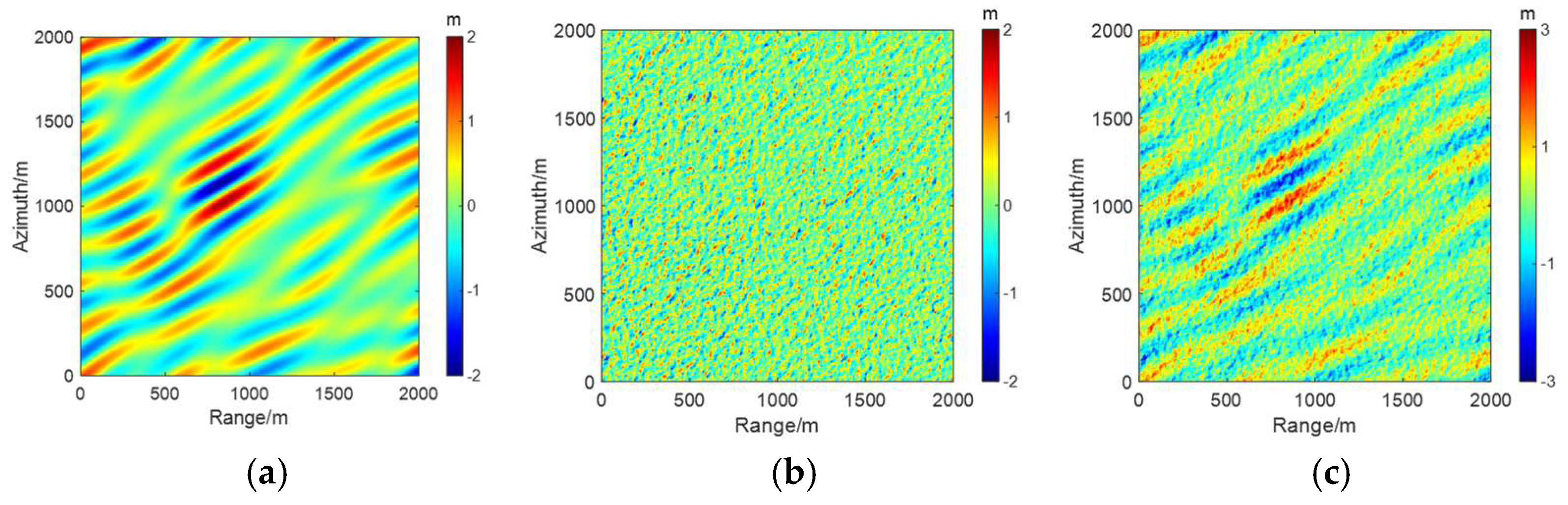
Based on the quasi-linear integral transform model between the phase spectrum and the ocean wave spectrum, we can conveniently obtain the corresponding phase spectrum from the ocean wave spectrum under certain conditions. To investigate the differences between the three quasi-linear integral transform models and the nonlinear integral transform model, we designed the following simulation-based difference evaluation experiments in this work.

(1) The Pierson–Moskowitz (PM) spectrum was used as the input for swell waves [37] and the Elfouhaily spectrum as the input for wind waves [38]. By employing the Monte Carlo method [39,40], the mathematical expressions for the PM spectrum and Elfouhaily spectrum are presented in Equations (27) and (28), respectively, with detailed parameter definitions for both expressions can be found in references [37,38].

$$S(k)={\displaystyle \frac{\alpha }{2k^3}}\exp \left(-{\displaystyle \frac{\beta g^2}{U_{19.5}^4{k}^2}}\right)$$

(27)

$$S\left(k\right)=0.5k^{-3}\left[{\alpha }_p{F}_{p}c\left(k_p\right)/c\left(k\right)+{\alpha }_m{F}_{m}c\left(k_m\right)/c\left(k\right)\right]$$

(28)

(2) Sea state condition parameters and XTI-SAR system configurations mainly include:

Wind speeds (U₁₀): 5 m/s, 8 m/s, 10 m/s, and 12 m/s.

Wind directions (WD): 0, 45°, and 90°.

Swell wavelengths (λ_s): 100 m, 150 m, 200 m, 250 m, and 300 m.

Incidence angles (θ): 30°, 40°, and 50°.

(3) On the basis of these simulated two-dimensional rough surfaces, as shown in Figure 4, the corresponding two-dimensional ocean wave spectra can be acquired. Subsequently, the differences between the quasi-linear integral transform models and the nonlinear integral transform model were analyzed based on the two-dimensional ocean wave spectrum. To quantitatively evaluate the differences between the quasi-linear integral transform models and the nonlinear integral transform model, we utilized the following three difference indicators for quantitative assessment [41,42]:

$$C={\displaystyle \frac{{\displaystyle \int P_{\phi nl}\left(k\right)P_{\phi ql}\left(k\right)dk}}{\sqrt{{\displaystyle \int P_{\phi nl}^2\left(k\right)dk}{\displaystyle \int P_{\phi ql}^2\left(k\right)dk}}}}$$

(29)

$$K={\displaystyle \frac{{\displaystyle \int \left|P_{\phi ql}\left(k\right)-P_{\phi nl}\left(k\right)\right|dk}}{{\displaystyle \int P_{\phi nl}\left(k\right)dk}}}$$

(30)

$$NLP=\sqrt{{\left({\displaystyle \frac{R}{V}}\right)}^2{f}^u\left(0\right)}{\displaystyle \frac{{\displaystyle \int P_{\phi nl}\left(k\right)\left|k_x\right|dk}}{{\displaystyle \int P_{\phi nl}\left(k\right)dk}}}$$

(31)

where $P_{\phi nl}\left(k\right)$ and $P_{\phi ql}\left(k\right)$ represent the phase spectra calculated using the nonlinear integral transform model and the quasi-linear integral transform model, respectively. The parameters C and K can be used to evaluate the correlation and bias between the quasi-linear phase spectrum and the nonlinear phase spectrum, respectively, and the parameter NLP can be used to evaluate the nonlinearity degree of the XTI-SAR system in ocean wave imaging.

3. Results

Compared with the traditional single-antenna SAR systems, establishing the integral transform models, including nonlinear and quasi-linear, between XTI-SAR ocean wave spectra and phase spectra represents a research endeavor of both profound theoretical significance and substantial practical value. This work constitutes a core scientific challenge for enabling high-precision ocean wave measurements using XTI-SAR technology. The model developments not only contribute to elucidating the imaging mechanisms of XTI-SAR in marine environments but also serve as the foundational framework for retrieving two-dimensional ocean wave directional spectra. A thorough investigation into how varying diverse sea state conditions and radar system parameters interactively influence XTI-SAR imaging performance holds dual strategic importance. First, it provides critical theoretical guidance for optimizing payload designs of future spaceborne interferometric SAR missions. Second, more significantly, it lays the theoretical foundation for the practical application of XTI-SAR in ocean dynamics environment monitoring.

3.1. The Influence of Wind Speed on the Difference

With the increase in wind speed, the correlation (C_ql1) between the first quasi-linear phase spectrum and the nonlinear phase spectrum initially decreases gradually and then gradually increases. Conversely, the bias (K_ql1) between the first quasi-linear phase spectrum and the nonlinear phase spectrum first increases gradually before diminishing. As shown in Figure 5, Figure 6 and Figure 7, the attenuation rate of the MTF along the azimuth direction intensifies with rising wind speeds, resulting in the gradual disappearance of the swell phase spectrum. Furthermore, after the disappearance of the swell phase spectrum, the spectra magnitude of the wind wave phase spectrum progressively increases with increasing wind speeds, and the proportion of the wind wave phase spectrum gradually strengthens. This results in a continuous reduction in the difference between the first quasi-linear phase spectrum and the nonlinear phase spectrum. Regarding the second quasi-linear integral transform and its optimized form, although the correlations (C_ql2 and C_ql2s) between these two quasi-linear phase spectra and the nonlinear phase spectrum exhibit a decreasing tendency with wind speed increases, while their corresponding biases (K_ql2 and K_ql2s) show an increasing trend, they still maintain relatively high correlations with the nonlinear phase spectrum. Moreover, these decreasing and increasing variation trends are significantly smaller than those of the first quasi-linear model. According to

Table 1. Parameters of SAR imaging of ocean waves and the differences between three quasi-linear phase spectra and nonlinear phase spectra under different wind speeds.

U10/(m/s)	WD/°	λs/m	SD/°	SWH/m	H/km	θ/°	—
	30	200	60	2	500	30	—
	Cql1	Cql2	Cql2s	Kql1	Kql2	Kql2s	NLP
5	0.97	0.99	0.99	0.48	0.25	0.30	0.94
8	0.42	1	1	0.86	0.31	0.34	1.29
10	0.31	0.99	0.99	0.73	0.43	0.37	1.40
12	0.79	0.96	0.98	0.62	0.46	0.37	1.38

Note: SD is the direction of swell propagation, and H is the height of platform.

and Figure 8, it can be found that as wind speed increases, the nonlinearity degree of SAR system ocean wave imaging initially progressively intensifies and subsequently gradually diminishes. For the SAR imaging configuration considered in this study, the nonlinearity degree reaches its maximum value of approximately 1.40 when the wind speed is around 10 m/s. To explain this phenomenon, we decomposed the nonlinearity calculation Equation (31) into three components: $\sqrt{{\left(R/V\right)}^2{f}^u\left(0\right)}$, ${\displaystyle \int P_{\phi nl}\left(k\right)\left|k_x\right|dk}$, and ${\displaystyle \int P_{\phi nl}\left(k\right)dk}$. As demonstrated in Figure 9a–c, component f^u(0) exhibits a positive correlation with wind speed, resulting in a monotonic increase of $\sqrt{{\left(R/V\right)}^2{f}^u\left(0\right)}$ with rising wind speeds. However, when we calculate ${\displaystyle \int P_{\phi nl}\left(k\right)\left|k_x\right|dk}$ and ${\displaystyle \int P_{\phi nl}\left(k\right)dk}$, we found that ${\displaystyle \int P_{\phi nl}\left(k\right)\left|k_x\right|dk}$ and ${\displaystyle \int P_{\phi nl}\left(k\right)dk}$ show a change of decreasing and then increasing with the increase of wind speeds, which is because the attenuation effect caused by the azimuth direction with velocity bunching has less influence on the ocean waves when the wind speed is small, thus preserving more ocean wave information. As wind speed increases beyond a certain threshold, the swell phase spectrum gradually diminishes, while wind waves progressively distribute toward lower wavenumber regions with increasing phase spectrum magnitude. Figure 9d illustrates the comparative analysis between $\sqrt{{\left(R/V\right)}^2{f}^u\left(0\right)}{\displaystyle \int P_{\phi nl}\left(k\right)\left|k_x\right|dk}$ and ${\displaystyle \int P_{\phi nl}\left(k\right)dk}$, revealing that the maximum discrepancy between these components occurs at the wind speed of 10 m/s, which corresponds to the maximum degree of nonlinearity occurring at this wind speed.

Additionally, among the three quasi-linear phase spectra, the first quasi-linear integral transform exhibits the maximum attenuation rate of the MTF along the azimuth direction. This results in the narrowest azimuth distribution of the first quasi-linear phase spectrum, consequently leading to the greatest difference with the nonlinear phase spectrum and thereby achieving the minimum correlation between them. The optimized second quasi-linear phase spectrum demonstrates a slightly broader azimuth distribution compared to its non-optimized counterpart. This phenomenon is primarily attributed to the optimized second quasi-linear integral transform, whose MTF exhibits a lower attenuation rate along the azimuth direction than that of the original second quasi-linear integral transform (refer to Figure 5a, Figure 6a and Figure 7a). Precisely due to this mechanism, the spectral magnitude of the optimized second quasi-linear phase spectrum becomes marginally higher than that of the original second quasi-linear phase spectrum.

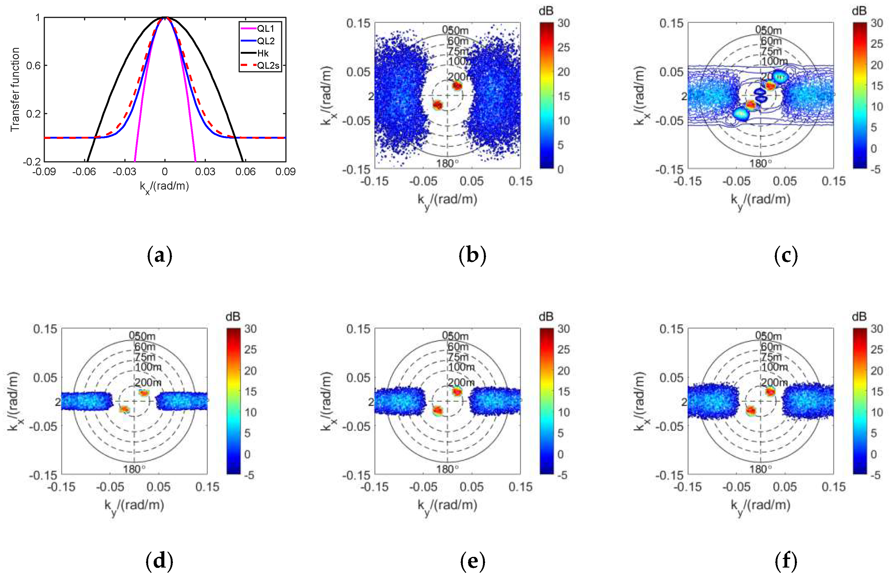
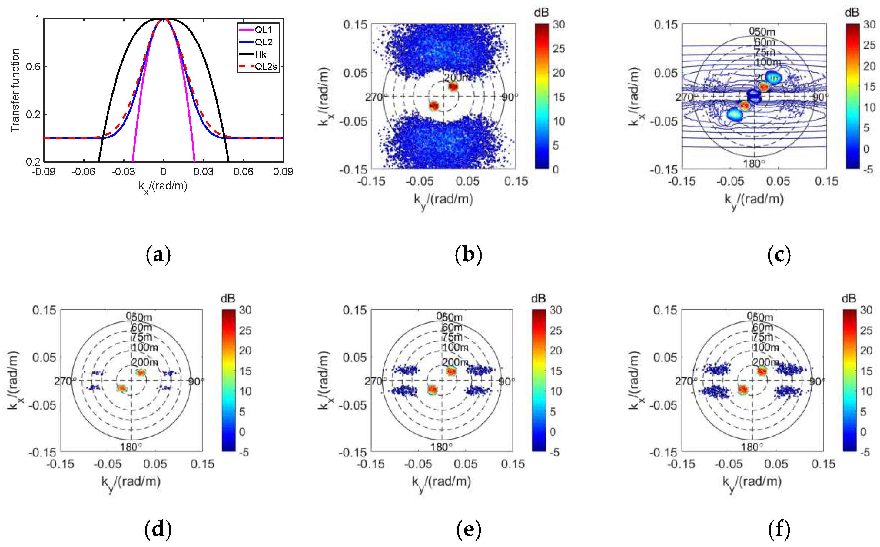
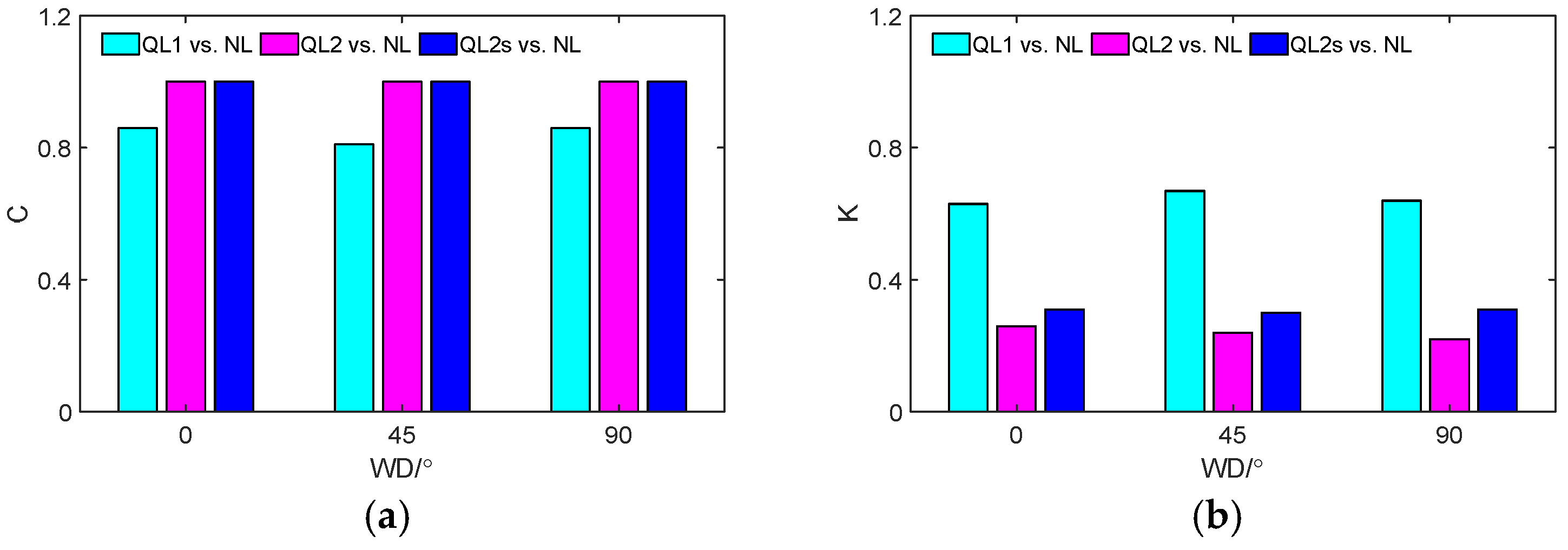
3.2. The Influence of Wind Direction on the Difference

As evidenced by Figure 10, Figure 11 and Figure 12, during the wind direction variation from 0° (range direction) to 90° (azimuth direction), the azimuth attenuation rates of the MTF in the three quasi-linear models exhibit no significant variation. This phenomenon is primarily due to the fact that when wind direction is the sole variable, the differences between |f^hu(0)| corresponding to different wind directions and the differences between f^u(0) corresponding to different wind directions are not significant. However, during the wind direction variation from 0° to 90°, the dominant wind wave direction correspondingly shifts from 0° to 90°. This direction realignment of dominant wind waves induces significant shape differences in the truncated phase spectra shaped by the MTF under varying wind directions. Concurrently, a pronounced reduction in spectral magnitude is observed, which can be fundamentally attributed to the wind wave energy redistribution caused by the progressive rotation of the dominant wind wave propagation axis. As indicated in

Table 2. Parameters of SAR imaging of ocean waves and the differences between three quasi-linear phase spectra and nonlinear phase spectra under different wind direction.

WD/°	U10/(m/s)	λs/m	SD/°	SWH/m	H/km	θ/°	—
	8	200	45	2	500	30	—
	Cql1	Cql2	Cql2s	Kql1	Kql2	Kql2s	NLP
0	0.86	1.00	1.00	0.63	0.26	0.31	1.09
45	0.81	1.00	1.00	0.67	0.24	0.30	1.12
90	0.86	1.00	1.00	0.64	0.22	0.31	1.18

and Figure 13, although the nonlinearity degree of SAR ocean wave imaging exhibits a gradual increasing trend with wind direction increases, the discrepancies between the three quasi-linear integral transforms and the nonlinear integral transform remain relatively stable. Moreover, among the three quasi-linear phase spectra, the first quasi-linear phase spectrum exhibits the largest discrepancy from its nonlinear counterpart, while both the second quasi-linear phase spectrum and its optimized version demonstrate substantially smaller deviations compared to the nonlinear phase spectrum. This primarily stems from the fact that the azimuth MTF of the first quasi-linear integral transform model exhibits the most rapid attenuation rate. This steep attenuation not only results in truncation of partial wind wave phase spectra along the azimuth direction but also causes the truncation of partial swell phase spectra in the same orientation. In contrast, the azimuth MTFs of the other two quasi-linear models have a more moderate attenuation rate, enabling better consistency between their phase spectra and the nonlinear phase spectra.

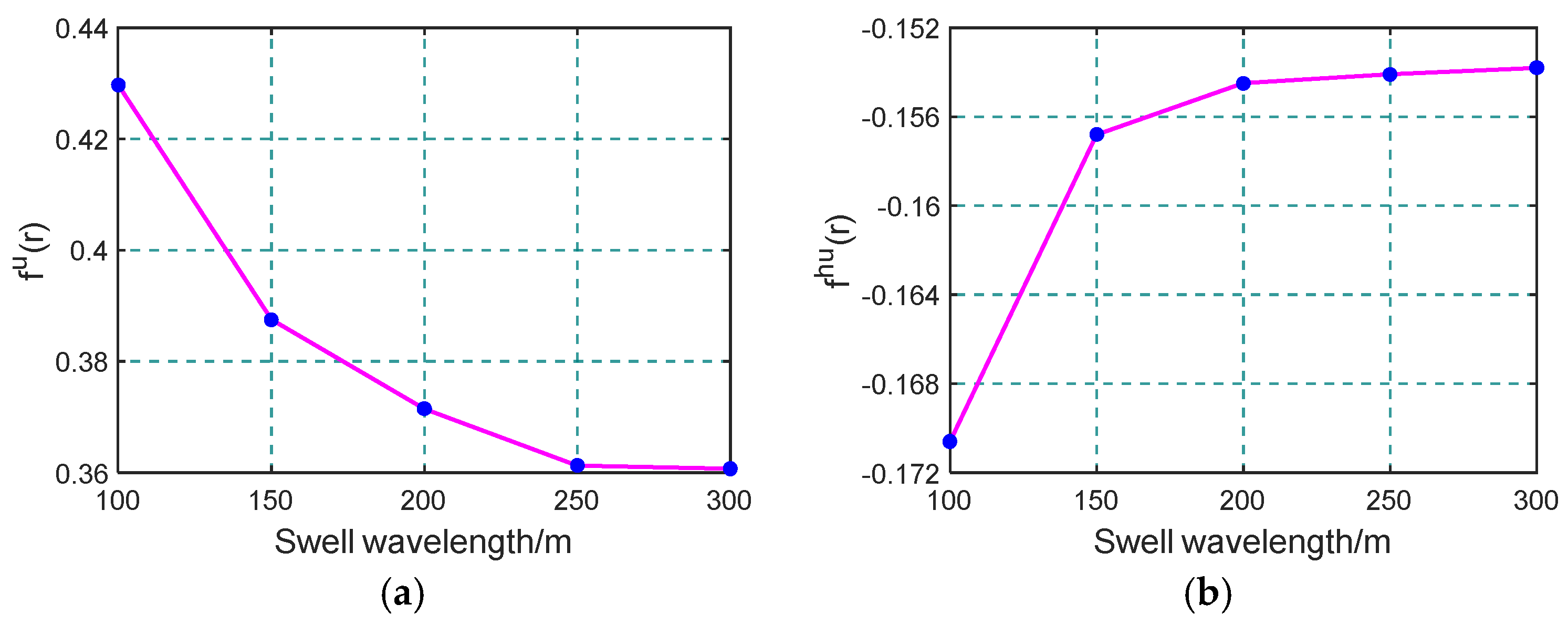
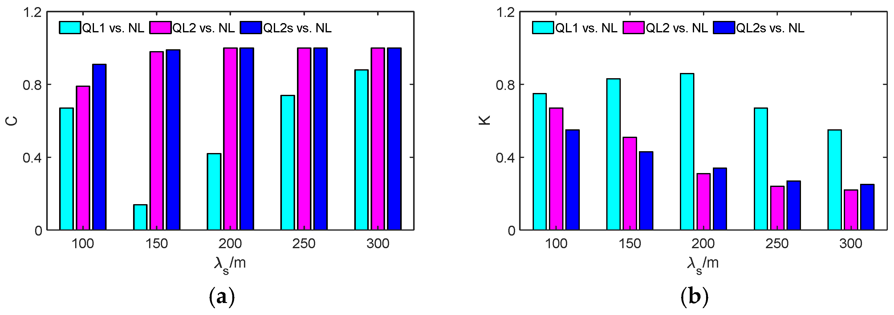
3.3. The Influence of Swell Wavelength on the Difference

As demonstrated in Figure 14, Figure 15 and Figure 16, the azimuth attenuation rates of the MTF in the three quasi-linear models show a slight reduction with increasing swell wavelength, which is mainly due to the fact that, under constant SWH conditions, the growth in swell wavelength induces a decrease in f^u(0), which, in turn, gradually reduces the attenuation rate of the attenuation function along the azimuth direction of the three quasi-linear functions. As indicated by Equations (17), (20) and (26), the MTFs of the three quasi-linear integral transform models are correlated with f^u(r)and f^hu(r). When maintaining constant SWH while increasing the swell wavelength, swell energy progressively redistributes toward lower wavenumber regions, accompanied by a gradual decrease in swell orbital velocity. Since wind wave parameters remain unchanged, this results in a gradual reduction in the magnitudes of f^u(r)and f^hu(r), as demonstrated in Figure 17. Furthermore, under typical conditions where wind wave orbital velocity significantly greater than that of swell orbital velocity, the influence of swell orbital velocity variations on f^u(r)and f^hu(r) becomes relatively insignificant when swell wave height remains constant and wavelength increases. Consequently, while the MTF attenuation rates of the three quasi-linear models exhibit a slight decreasing trend, this decreasing trend is not significant.

As shown in

Table 3. Parameters of SAR imaging of ocean waves and the differences between three quasi-linear phase spectra and nonlinear phase spectra under different swell wavelengths.

λs/m	U10/(m/s)	WD/°	SD/°	SWH/m	H/km	θ/°	—
	8	30	60	2	500	30	—
	Cql1	Cql2	Cql2s	Kql1	Kql2	Kql2s	NLP
100	0.67	0.79	0.91	0.75	0.67	0.55	1.76
150	0.14	0.98	0.99	0.83	0.51	0.43	1.55
200	0.42	1	1	0.86	0.31	0.34	1.29
250	0.74	1	1	0.67	0.24	0.27	1.09
300	0.88	1	1	0.55	0.22	0.25	1.01

and Figure 18, for the first quasi-linear model, the difference between it and the nonlinear phase spectrum first increases and then decreases with the increase of swell wavelength. This is mainly because the MTF of the first quasi-linear model has a large attenuation rate along the azimuth direction. When the swell wavelength is small, the swell phase spectrum in the first quasi-linear phase spectrum is completely truncated and lost. As the swell wavelength increases, the swell phase spectrum is concentrated in a smaller wavenumber range, and the attenuation rate of the MTF along the azimuth direction is relatively small, so the proportion of the swell phase spectrum retained in the first quasi-linear phase spectrum gradually increases. Exactly because of this mechanism, both the second quasi-linear model and its optimized counterpart exhibit progressively diminishing discrepancies from the nonlinear phase spectrum with increasing swell wavelength. Furthermore, the nonlinearity degree of SAR ocean wave imaging demonstrates a gradual reduction as swell wavelength augments, a phenomenon arising from dual mechanistic origins. The first is that as the swell wavelength increases, f^u(0) gradually decreases. However, after the swell wavelength increases to a certain extent, f^u(0) tends to stabilize. Secondly, it can be found from Equation (31) that the nonlinearity of SAR ocean waves imaging gradually decreases because the swell phase spectrum is concentrated in a smaller wavenumber range.

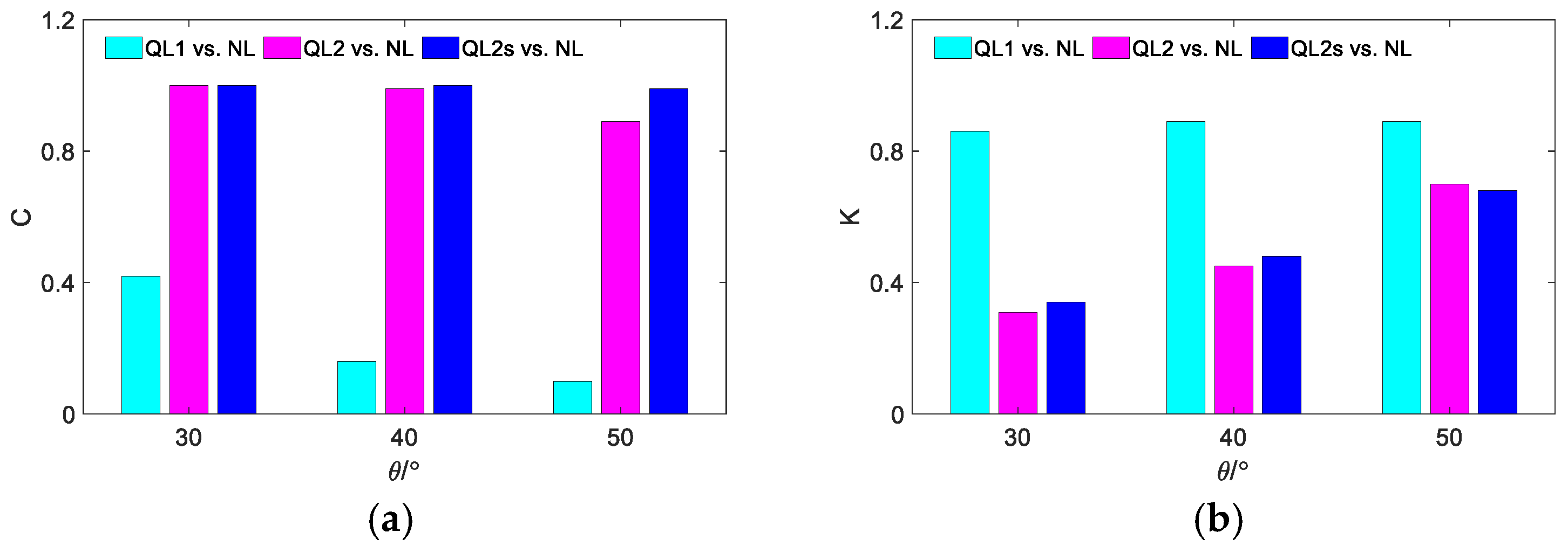
3.4. The Influence of Incidence Angle on the Difference

As revealed in Figure 19, Figure 20 and Figure 21, the azimuth attenuation rates of the MTF in the three quasi-linear models exhibit significant increase with increasing incidence angle θ, resulting in a contraction of the wavenumber domain for phase spectrum distribution along the azimuth direction. This phenomenon is mainly due to the progressive increase of the parameter β = R/V induced by the increased θ, which consequently enhances the nonlinear coupling effects between the phase spectrum and the ocean wave spectrum. As can be seen from

Table 4. SAR imaging parameters of ocean waves and the differences between three quasi-linear phase spectra and nonlinear phase spectra under different incidence angles.

θ/°	U10/(m/s)	WD/°	λs/m	SD/°	SWH/m	H/km	—
	8	30	200	60	2	500	—
	Cql1	Cql2	Cql2s	Kql1	Kql2	Kql2s	NLP
30	0.42	1.00	1.00	85.88	31.12	33.71	1.29
40	0.16	0.99	1.00	89.22	45.08	48.04	1.44
50	0.10	0.89	0.99	88.54	69.74	68.32	1.72

and Figure 22, the progressive increase in θ induces a corresponding increase in the parameter β, thereby enhancing the nonlinearity between the phase spectrum and the ocean wave spectrum. It is precisely due to this enhanced nonlinearity in the conversion relationship between the phase spectrum and the ocean wave spectrum that the difference between the nonlinear phase spectrum and the three quasi-linear phase spectra increases.

3.5. Applicability Analysis of the Quasi-Linear Models

As shown in Table 1, Table 2, Table 3 and Table 4, generally, for most sea state conditions and XTI-SAR system configurations, the second quasi-linear integral transform model and its optimized form exhibit minimal discrepancies compared to the nonlinear integral transform model, which indicate that the two models have high applicability. For the first quasi-linear integral transform model, its applicability is primarily influenced by wind speeds. Generally, since wind wave orbital velocity exhibits a strong correlation with wind speeds, and wind wave orbital velocity is typically significantly greater than that of swells. Consequently, azimuth truncation caused by velocity bunching is predominantly governed by wind waves. Under low wind speed conditions (U₁₀ < 5 m/s), the attenuation rate of the azimuth MTF is relatively small, allowing more ocean wave spectral information to be preserved. In contrast, under high wind speeds (U₁₀ > 12 m/s), although the azimuth MTF attenuation rate increases, a larger proportion of wave energy becomes concentrated in the low wavenumber regions, thereby reducing the sensitivity of the first quasi-linear model to wind speed variations. As a result, the first quasi-linear model demonstrates high applicability under both low and high wind speed conditions.

4. Conclusions

In order to better understand the imaging mechanism of the XTI-SAR system for ocean waves, in this work a series of studies were conducted based on the existing integral transform models between the phase spectrum and the ocean wave spectrum.

Firstly, based on the nonlinear integral transform model between the XTI-SAR phase spectrum and the ocean wave spectrum established by Bao in 1999, this work theoretically derives a quasi-linear integral transform model between the phase spectrum and the ocean wave spectrum, and also optimizes another quasi-linear integral transform model derived by Bao, so as to obtain a total of three quasi-linear integral transform models at present. In terms of form, the optimized quasi-linear integral transforms are more concise and convenient when using the ocean wave spectrum to calculate the phase spectrum.

Secondly, in order to investigate the differences between the three quasi-linear integral transform models and the nonlinear integral transform model, the PM spectrum was employed here as the input spectrum for swell simulation and the Elfouhaily spectrum for wind wave simulation, and used the Monte Carlo method to simulate the two-dimensional sea surface under multiple parameters to carry out the differences for quantitative analysis. The research results show that since the quasi-linear integral transform model derived in this work has a severe truncation effect in the azimuth direction, the difference between this quasi-linear integral transform model and the nonlinear integral transform model is generally large under different sea states and different imaging conditions. However, the differences between the other two quasi-linear integral transform models, namely the quasi-linear integral transform model derived by Bao and the optimized model in this study, and the nonlinear integral transform model are relatively small. In terms of performance, the optimized quasi-linear integral transform model demonstrates superior capabilities compared to both the first and second quasi-linear integral transform models under most scenarios. Therefore, for practical image analysis applications, we strongly recommend adopting the optimized quasi-linear integral transform model proposed in this work. In addition, in general, the differences between the three quasi-linear integral transform models and the nonlinear integral transform model are proportional to the nonlinearity degree in the SAR imaging process of ocean waves.

References

1. Xiang, C.; Zhang, K.; Li, M.; Yang, F.; Xu, S. Three-Dimensional Modeling for Ocean Electromagnetic Environment. In Proceedings of the 2020 IEEE International Symposium on Antennas and Propagation and North American Radio Science Meeting, Montreal, QC, Canada, 5–10 July 2020. [Google Scholar]
2. Gao, H.; Liang, B.; Shao, Z. A global climate analysis of wave parameters with a focus on wave period from 1979 to 2018. Appl. Ocean Res. 2021, 111, 102652. [Google Scholar] [CrossRef]
3. Gao, Y.; Kamenkovich, I.; Perlin, N.; Kirtman, B. Oceanic Advection Controls Mesoscale Mixed Layer Heat Budget and Air–Sea Heat Exchange in the Southern Ocean. J. Phys. Oceanogr. 2022, 52, 537–555. [Google Scholar] [CrossRef]
4. Li, S.; Yu, H.; Wu, K.; Yin, X.; Lang, S.; Ye, J. Validation of the Ocean Wave Spectrum from the Remote Sensing Data of the Chinese–French Oceanography Satellite. Remote Sens. 2023, 15, 3918. [Google Scholar] [CrossRef]
5. Zhang, X.; Su, X.; Liu, L.; Wu, Z. Experimental Investigation of Meter-Level Resolution Radar Measurement at Ka Band in Yellow Sea. Remote Sens. 2024, 16, 3835. [Google Scholar] [CrossRef]
6. Matos, T.; Rocha, J.L.; Martins, M.S.; Gonçalves, L.M. Enhancing Sea Wave Monitoring Through Integrated Pressure Sensors in Smart Marine Cables. J. Mar. Sci. Eng. 2025, 13, 766. [Google Scholar] [CrossRef]
7. Martínez-Rodrigo, R.; Águeda, B.; Lopez-Sanchez, J.M.; Altelarrea, J.M.; Alejandro, P.; Gómez, C. Exploring the Relationship Between Time Series of Sentinel-1 Interferometric Coherence Data and Wild Edible Mushroom Yields in Mediterranean Forests. J. Geovis. Spat. Anal. 2024, 8, 38. [Google Scholar] [CrossRef]
8. Elyouncha, A.; Eriksson, L.E.B.; Romeiser, R.; Ulander, L.M.H. Measurements of Sea Surface Currents in the Baltic Sea Region Using Spaceborne Along-Track InSAR. IEEE Trans. Geosci. Remote Sens. 2019, 57, 8584–8599. [Google Scholar] [CrossRef]
9. An, S.; Han, S.; Kim, D.J. Enhancing SAR ATR Accuracy for Military Targets: A Novel Approach Using XTI and Amplitude Data Integration. IEEE Geosci. Remote Sens. Lett. 2024, 22, 4001705. [Google Scholar] [CrossRef]
10. Zhang, J.B.; Duan, W.; Fu, X.K. The Stepwise Multi-Temporal Interferometric Synthetic Aperture Radar with Partially Coherent Scatterers for Long-Time Series Deformation Monitoring. Remote Sens. 2025, 17, 1374. [Google Scholar] [CrossRef]
11. Marom, M.; Goldstein, R.M.; Thornton, E.B.; Shemer, L. Remote Sensing of Ocean Wave Spectra by Interferometric Synthetic Aperture Radar. Nature 1990, 345, 793–795. [Google Scholar] [CrossRef]
12. Chen, Y.; Huang, M.; Zhang, Y.; Wang, C.; Duan, T. An Analytical Method for Dynamic Wave—Related Errors of Interferometric SAR Ocean Altimetry under Multiple Sea States. Remote Sens. 2021, 13, 986. [Google Scholar] [CrossRef]
13. Shemer, L. Interferometric SAR imagery of a monochromatic ocean wave in the presence of the real aperture radar modulation. Int. J. Remote Sens. 1993, 14, 3005–3019. [Google Scholar] [CrossRef]
14. Zhang, B.; He, Y.J. A Parametric Algorithm to Retrieve Ocean Wave Spectra from Interferometric Synthetic Aperture Radar. In Proceedings of the IGARSS 2008—2008 IEEE International Geoscience and Remote Sensing Symposium, Boston, MA, USA, 7–11 July 2008; pp. 424–427. [Google Scholar]
15. Bao, M. A nonlinear integral transform between ocean wave spectra and phase image spectra of a cross-track interferometric SAR. In Proceedings of the 1999 IEEE International Geoscience and Remote Sensing Symposium, Hamburg, Germany, 28 June–2 July 1999; Volume 5, pp. 2619–2621. [Google Scholar]
16. Schulz-Stellenfleth, J.; Lehner, S. Ocean wave imaging using an airborne single pass across-track interferometric synthetic aperture radar. IEEE Trans. Geosci. Remote Sens. 2001, 39, 38–45. [Google Scholar] [CrossRef]
17. Schulz-Stellenfleth, J.; Horstmann, J.; Lehner, S.; Rosenthal, W. Sea surface imaging with an across track interferometric synthetic aperture radar---The SINEWAVE experiment. IEEE Trans. Geosci. Remote Sens. 2001, 39, 2017–2028. [Google Scholar] [CrossRef]
18. Zhang, B.; He, Y.J. Interferometric phase model and numerical simulations of swell for across-track interferometric SAR. Chin. J. Radio Sci. 2007, 22, 1014–1028. [Google Scholar]
19. Vaze, P.; Kaki, S.; Limonadi, D.; Esteban-Fernandez, D.; Zohar, G. The Surface Water and Ocean Topography Mission. In Proceedings of the 2018 IEEE Aerospace Conference, Big Sky, MT, USA, 3–10 March 2018. [Google Scholar]
20. Yao, J.; Xu, N.; Wang, M.; Liu, T.; Lu, H.; Cao, Y.; Tang, X.; Mo, F.; Chang, H.; Gong, H.; et al. SWOT satellite for global hydrological applications: Accuracy assessment and insights into surface water dynamics. Int. J. Digit. Earth 2025, 18, 2472924. [Google Scholar] [CrossRef]
21. Rodriguez, E.; Esteban-Fernandez, D. The Surface Water and Ocean Topography Mission (SWOT): The Ka-band Radar Interferometer (KaRIn) for water level measurements at all scales. In Proceedings of the SPIE Remote Sensing, Toulouse, France, 20–23 September 2010; Volume 7826, pp. 1–8. [Google Scholar]
22. Neeck, S.P.; Lindstrom, E.J.; Vaze, P.V.; Fu, L.L. Surface Water and Ocean Topography (SWOT) mission. In Proceedings of the SPIE Remote Sensing, Edinburgh, UK, 24–27 September 2012. [Google Scholar]
23. Chen, G.; Tang, J.; Zhao, C.; Wu, S.; Yu, F.; Ma, C.; Xu, Y.; Chen, W.; Zhang, Y.; Liu, J.; et al. Concept Design of the “Guanlan” Science Mission: China’s Novel Contribution to Space Oceanography. Front. Mar. Sci. 2019, 6, 194. [Google Scholar] [CrossRef]
24. Yang, L.; Xu, Y.; Zhou, X.; Zhu, L.; Jiang, Q.; Sun, H.; Chen, G.; Wang, P.; Mertikas, S.P.; Fu, Y.; et al. Calibration of an Airborne Interferometric Radar Altimeter over the Qingdao Coast Sea, China. Remote Sens. 2020, 12, 1651. [Google Scholar] [CrossRef]
25. Jiang, Q.; Xu, Y.; Sun, H.; Wei, L.; Yang, L.; Zheng, Q.; Jiang, H.; Zhang, X.; Qian, C. Wind-generated gravity waves retrieval from high-resolution 2-D maps of sea surface elevation by airborne interferometric altimeter. IEEE Geosci. Remote Sens. Lett. 2021, 19, 1–5. [Google Scholar] [CrossRef]
26. Ma, C.; Pan, L.; Qiu, Z.; Liang, D.; Chen, G.; Yu, F.; Sun, H.; Sun, D.; Wu, W. Ocean Wave Inversion Based on a Ku/Ka Dual-Band Airborne Interferometric Imaging Radar Altimeter. Remote Sens. 2022, 14, 3578. [Google Scholar] [CrossRef]
27. Qiu, Z.; Ma, C.; Wang, Y.; Yu, F.; Zhao, C.; Sun, H.; Zhao, S.; Yang, L.; Tang, J.; Chen, G. Improving Sea Surface Height Reconstruction by Simultaneous Ku- and Ka-Band Near-Nadir Single-Pass Interferometric SAR Altimeter. IEEE Trans. Geosci. Remote Sens. 2023, 61, 5209614. [Google Scholar] [CrossRef]
28. Sun, D.; Zhang, Y.; Wang, Y.; Chen, G.; Sun, H.; Yang, L.; Bai, Y.; Yu, F.; Zhao, C. Ocean Wave Inversion Based on Airborne IRA Images. IEEE Trans. Geosci. Remote Sens. 2022, 60, 1001013. [Google Scholar] [CrossRef]
29. Sun, D.; Wang, Y.; Xu, Z.; Zhang, Y.; Zhang, Y.; Meng, J.; Sun, H.; Yang, L. Ocean wave inversion based on hybrid along- and crosstrack interferometry. Remote Sens. 2022, 14, 2793. [Google Scholar] [CrossRef]
30. Stoffelen, A.; Anderson, D. Scatterometer data interpretation: Estimation and validation of the transfer function CMOD4. J. Geophys. Res. Ocean. 1997, 102, 5767–5780. [Google Scholar] [CrossRef]
31. Raney, R. Synthetic aperture imaging radar and moving targets. IEEE Trans. Aerosp. Electron. Syst. 1971, AES-7, 499–505. [Google Scholar]
32. Sun, D.; Wang, Y.; Zhang, Y.; Sun, H.; Yang, L.; Yu, F. Wind wave and wind speed inversion based on azimuth cutoff of airborne IRA images. IEEE Trans. Geosci. Remote Sens. 2024, 62, 4201914. [Google Scholar] [CrossRef]
33. Bao, M.Q.; Alpers, W. A new nonlinear integral transform relating ocean wave spectra to phase image spectra of an along-track interferometric synthetic aperture radar. IEEE Trans. Geosci. Remote Sens. 1999, 37, 461–466. [Google Scholar]
34. Krogstad, H.E. A simple derivation of Hasselmann’s nonlinear ocean-synthetic aperture radar transform. J. Geophys. Res. Ocean. 1992, 97, 873–885. [Google Scholar] [CrossRef]
35. Parzen, E. Stochastic Processes; Holden-Day: San Francisco, CA, USA, 1962; Volume 324. [Google Scholar]
36. Hasselmann, K.; Hasselmann, S. On the nonlinear mapping of an ocean wave spectrum into a synthetic aperture radar image spectrum and its inversion. J. Geophys. Res. 1991, 96, 10713–10729. [Google Scholar] [CrossRef]
37. Pierson, W.J.; Moskowitz, L. A proposed spectral form for fully developed wind seas based on the similarity theory of SA Kitaigorodskii. J. Geophys. Res. 1964, 69, 5181–5190. [Google Scholar] [CrossRef]
38. Elfouhaily, T.; Chapron, B.; Katsaros, K.; Vandemark, D. A unified directional spectrum for long and short wind-driven waves. J. Geophys. Res. Ocean. 1997, 102, 15781–15796. [Google Scholar] [CrossRef]
39. Alpers, W.R. Monte Carlo simulations for studying the relationship between ocean wave and synthetic aperture radar image spectra. J. Geophys. Res. 1983, 88, 1745–1759. [Google Scholar] [CrossRef]
40. Bruning, C.; Alpers, W.R.; Hasselmann, K. Monte-Carlo simulation studies of the nonlinear imaging of a two dimensional surface wave field by a synthetic aperture radar. Int. J. Remote Sens. 1990, 11, 1695–1727. [Google Scholar] [CrossRef]
41. He, Y.J.; Alpers, W. On the nonlinear integral transform of an ocean wave spectrum into an along-track interferometric synthetic aperture radar image spectrum. J. Geophys. Res. Atmos. 2003, 108, 3205. [Google Scholar] [CrossRef]
42. Vachon, P.W.; Campbell, J.W.; Gray, A.L.; Dobson, F.W. Validation of along-track interferometric SAR measurements of ocean surface waves. IEEE Trans. Geosci. Remote Sens. 1999, 37, 150–162. [Google Scholar] [CrossRef]
Figure 1. Geometric diagram of XTI-SAR system height measurement.
Remotesensing 17 01790 g001
Figure 2. The variation of the second quasi-linear model MTF ( Q L 2 = H ± k X 2 ), the optimized second quasi-linear model MTF ( Q L 2 s = exp k x 2 R 2 / V 2 f u 0 ), and Hk along the azimuth direction.
Remotesensing 17 01790 g002
Figure 3. The variation of the first quasi-linear model MTF (QL1), the second quasi-linear model MTF (QL2), and the optimized second quasi-linear model MTF (QL2s) along the azimuth direction.
Remotesensing 17 01790 g003
Figure 4. Two-dimensional sea surface heights simulated using PM spectra, Elfouhaily spectra, and Monte Carlo methods. (a) Swell, (b) wind waves, (c) combination of swell wind waves.
Remotesensing 17 01790 g004
Figure 5. Quasi-linear integral transform azimuth MTF corresponding to U10 = 5 m/s (a), ocean wave spectrum (b), nonlinear phase spectrum (c), phase spectrum of QL1 (d), phase spectrum of QL2 (e), phase spectrum of QL2s (f).
Remotesensing 17 01790 g005
Figure 6. Quasi-linear integral transform azimuth MTF corresponding to U10 = 8 m/s (a), ocean wave spectrum (b), nonlinear phase spectrum (c), phase spectrum of QL1 (d), phase spectrum of QL2 (e), phase spectrum of QL2s (f).
Remotesensing 17 01790 g006
Figure 7. Quasi-linear integral transform azimuth MTF corresponding to U10 = 12 m/s (a), ocean wave spectrum (b), nonlinear phase spectrum (c), phase spectrum of QL1 (d), phase spectrum of QL2 (e), phase spectrum of QL2s (f).
Remotesensing 17 01790 g007
Figure 8. Comparison of differences between three quasi-linear integral transform models and nonlinear integral transform models under different U10. (a) indicator C, (b) indicator K.
Remotesensing 17 01790 g008
Figure 9. Variation of R / V 2 f u 0 (a), P φ n l k k x d k (b) and P φ n l k d k (c) with wind speeds, comparison of R / V 2 f u 0 P φ n l k k x d k and P φ n l k d k with wind speeds (d).
Remotesensing 17 01790 g009
Figure 10. Quasi-linear integral transform azimuth MTF corresponding to WD = 0° (a), ocean wave spectrum (b), nonlinear phase spectrum (c), phase spectrum of QL1 (d), phase spectrum of QL2 (e), phase spectrum of QL2s (f).
Remotesensing 17 01790 g010
Figure 11. Quasi-linear integral transform azimuth MTF corresponding to WD = 45° (a), ocean wave spectrum (b), nonlinear phase spectrum (c), phase spectrum of QL1 (d), phase spectrum of QL2 (e), phase spectrum of QL2s (f).
Remotesensing 17 01790 g011
Figure 12. Quasi-linear integral transform azimuth MTF corresponding to WD = 90° (a), ocean wave spectrum (b), nonlinear phase spectrum (c), phase spectrum of QL1 (d), phase spectrum of QL2 (e), phase spectrum of QL2s (f).
Remotesensing 17 01790 g012
Figure 13. Comparison of differences between three quasi-linear integral transform models and nonlinear integral transform models under different WD. (a) indicator C, (b) indicator K.
Remotesensing 17 01790 g013
Figure 14. Quasi-linear integral transform azimuth MTF corresponding to λs = 100 m (a), ocean wave spectrum (b), nonlinear phase spectrum (c), phase spectrum of QL1 (d), phase spectrum of QL2 (e), phase spectrum of QL2s (f).
Remotesensing 17 01790 g014
Figure 15. Quasi-linear integral transform azimuth MTF corresponding to λs = 200 m (a), ocean wave spectrum (b), nonlinear phase spectrum (c), phase spectrum of QL1 (d), phase spectrum of QL2 (e), phase spectrum of QL2s (f).
Remotesensing 17 01790 g015
Figure 16. Quasi-linear integral transform azimuth MTF corresponding to λs = 300 m (a), ocean wave spectrum (b), nonlinear phase spectrum (c), phase spectrum of QL1 (d), phase spectrum of QL2 (e), phase spectrum of QL2s (f).
Remotesensing 17 01790 g016
Figure 17. Variation of fu(r) (a) and fhu(r) (b) with swell wavelengths.
Remotesensing 17 01790 g017
Figure 18. Comparison of differences between three quasi-linear integral transform models and nonlinear integral transform models under different swell wavelengths. (a) indicator C, (b) indicator K.
Remotesensing 17 01790 g018
Figure 19. Quasi-linear integral transform azimuth MTF corresponding to θ = 30° (a), ocean wave spectrum (b), nonlinear phase spectrum (c), phase spectrum of QL1 (d), phase spectrum of QL2 (e), phase spectrum of QL2s (f).
Remotesensing 17 01790 g019
Figure 20. Quasi-linear integral transform azimuth MTF corresponding to θ = 40° (a), ocean wave spectrum (b), nonlinear phase spectrum (c), phase spectrum of QL1 (d), phase spectrum of QL2 (e), phase spectrum of QL2s (f).
Remotesensing 17 01790 g020
Figure 21. Quasi-linear integral transform azimuth MTF corresponding to θ = 50° (a), ocean wave spectrum (b), nonlinear phase spectrum (c), phase spectrum of QL1 (d), phase spectrum of QL2 (e), phase spectrum of QL2s (f).
Remotesensing 17 01790 g021
Figure 22. Comparison of differences between three quasi-linear integral transform models and nonlinear integral transform models under different incidence angles. (a) indicator C, (b) indicator K.
Remotesensing 17 01790 g022