Remote Sensing of Particle Absorption Coefficient of Pigments Using a Two-Stage Framework Integrating Optical Classification and Machine Learning

Abstract

The particle absorption coefficient of pigments (a_ph(λ)), a critical indicator of phytoplankton spectral absorption properties, is essential for bio-optical models and water quality monitoring. To enhance the accuracy of a_ph(λ) retrieval in complex aquatic environments, this study proposes a novel two-stage framework integrating optical classification and machine learning regression. Focusing on inland waters—key areas for eutrophication monitoring—we first developed an intelligent clustering method combining Kernel Principal Angle-based Component (KPAC) dimensionality reduction and Chameleon Swarm Algorithm (CSA)-optimized k-medoids to classify water bodies into four optical types based on hyperspectral reflectance features. Subsequently, an XGBoost regression model with L1-norm feature selection was applied to inversely derive a_ph(440), a_ph(555), a_ph(675), and a_ph(709) for each class. Experimental results demonstrated that optical classification significantly improved inversion accuracy: the determination coefficients R² all exceeded 0.9 in classified datasets, with RMSE reduced by up to 93.1% compared to unclassified scenarios. This indicates that the strategy based on optical classification and regression inversion can effectively enhance the accuracy of pigment particle absorption coefficient inversions. In summary, this study, with the central objective of accurately measuring the pigment particle absorption coefficient, successfully developed a comprehensive set of optical classification and regression inversion methods applicable to various aquatic environments. This new scientific approach and powerful tool provide a means for monitoring and interpreting the pigment particle absorption characteristics in water bodies using remote sensing technology.

1. Introduction

With the rapid development of industrialization and urbanization, there has been a continuous increase in nutrient substances in water bodies, leading to an increasingly severe problem of eutrophication [1]. Phytoplankton, as the primary producers within aquatic ecosystems, have their biomass and absorption coefficients closely related to the degree of eutrophication [2]. By investigating phytoplankton absorption coefficients, one can gain insights into the composition and abundance of algae in water bodies, thereby assessing the ecological balance status and the level of eutrophication. Moreover, due to their dominance in downwelling light attenuation and significant role in energy transfer processes, phytoplankton absorption coefficients (a_ph(λ)) constitute a substantial proportion in the optical absorption changes of seawater (or lake water) [3,4], providing essential input parameters for biological optical models [5]. This enables more accurate simulations of light propagation in water, rendering phytoplankton absorption coefficients a critical inherent optical property in water color studies that is vital for constructing biological optical models and indirectly inferring water quality parameters such as chlorophyll-a [6]. Therefore, research on pigment particle absorption coefficients holds significant importance for monitoring, evaluating the nutrient status of lake and reservoir water bodies, maintaining the health of aquatic ecosystems, and implementing corresponding management measures [7].

1.1. Remote Sensing Inversion Methods for a_ph(λ)

Pigment particulate absorption coefficient remote sensing monitoring is a process that involves inferring the optical absorption characteristics of pigment particles at different wavelengths through the analysis of water color data [8]. In current research, the pigment particulate absorption coefficient (a_ph(λ)) serves as a critical component of water body optical properties and is widely employed in remote sensing monitoring to enhance estimations of other water color parameters such as chlorophyll-a concentrations, suspended matter concentrations, and colored dissolved organic matter, among others.

1.1.1. Empirical and Semi-Analytical Approaches

For instance, Jiang Guangjia et al. [9] classified the waters of the Pearl River Estuary based on IOCCG guidelines using non-pigment particulate absorption coefficients (a_d(λ)), pigment particulate absorption coefficients (a_ph(λ)), and CDOM absorption coefficients (a_g(λ)). They then established a remote sensing estimation model for phytoplankton absorption coefficients at 665 nm for each water type, enabling the inversion of particulate organic carbon and its endogenous and exogenous concentrations. Matsushita et al. [10], leveraging the relationship between MCI (maximum chlorophyll index) and chlorophyll concentration, set up MCI thresholds to categorize multiple lakes across Asia into water types with varying turbidity. They used multi-band algorithms to estimate chlorophyll concentrations separately for each water type, demonstrating the advantage of employing multiple algorithm models tailored to different water types. Jiang et al. [11] constructed a chlorophyll index (CI) utilizing the ratio of phytoplankton absorption coefficient at 443 nm to non-pigment particulate absorption coefficient, creating an index applicable to diverse water types. By combining this index with specific reflectance features at certain bands, they successfully improved the accuracy of remotely sensed data in estimating chlorophyll-a concentrations in different water bodies. Bricaud et al. [12], upon analyzing extensive datasets from oligotrophic, mesotrophic, and eutrophic water bodies, discovered a power law relationship between the phytoplankton absorption coefficient a_ph(440) and Chl-a.

1.1.2. Limitations of Existing Models

However, there has been relatively limited research on the direct remote sensing monitoring of pigment particulate absorption coefficients. Xu et al. [13] utilized the MCI index to categorize water bodies into highly turbid, moderately turbid, and clear waters, based on which they established a remote sensing estimation model for phytoplankton absorption coefficients at 665 nm. Hu et al. [14] tested the applicability of the Quasi-Analytical Algorithm (QAA) in the Yellow Sea using field-measured datasets. The results indicated that QAA performed satisfactorily in retrieving total absorption coefficients, yellow substance absorption coefficients, and detrital absorption coefficients in the Yellow Sea’s coastal waters; however, its performance was less than ideal for phytoplankton absorption coefficients. For instance, Lee et al. [15] developed the QAA for retrieving inherent optical properties of water bodies. This algorithm involves a seven-step process utilizing remote sensing reflectance data, incorporating two empirical models, two analytical methods, and three semi-analytical models [16]. They have made multiple refinements to this algorithm tailored to different water types, leading to the introduction of QAA_v4, QAA_v5, and QAA_v6 [17,18,19]. Models for inversely deriving absorption coefficients from remote sensing reflectance are not only applicable to a single type of water body but also suitable for situations where yellow substances and chlorophyll independently vary [20].

1.2. Water Optical Classification Techniques

In current studies, one optimization approach for remotely sensing phytoplankton absorption coefficients is through the use of water optical classification methods [21,22]. Specifically, this involves improving inversion model parameter selection and algorithm design by leveraging optical classification, thereby adapting to varying aquatic environmental conditions and enhancing the accuracy of water quality parameter estimation.

1.2.1. Classification Based on Bio-Optical and Inherent Properties

Li et al. [23] highlighted that, for complex inland and nearshore waters, the optical classification based on water body characteristics can more accurately characterize the influence of phytoplankton on water optical properties, upon which they built a phytoplankton absorption coefficient inversion model suitable for various types of water bodies. Le et al. [24] employed the normalized unit absorption coefficient of phytoplankton a_ph(λ) to classify water bodies and, based on these classifications, constructed a remote sensing estimation model for phytoplankton absorption coefficients at 665 nm. This model was further used to retrieve particulate organic carbon concentrations as well as their endogenous and exogenous sources.

Establishing water optical classification methods based on the optical characteristics of water bodies and subsequently constructing inversion models for water environmental parameters for each type of water optical category not only enhances the inversion accuracy of models within similar water body types but also facilitates their application in analogous environments. This is an effective approach to addressing the significant spatial and temporal differences in water body environments near inland and coastal areas, as well as the relatively low universality of existing models [25].

1.2.2. Challenges in Classification Criteria

The process of water optical clustering involves grouping spectral data into clusters according to the natural distribution properties of surface spectra, where spectral variables exhibit varying degrees of similarity or relatedness; these are clustered under certain criteria to determine the water optical classification [23]. Water optical classification primarily relies on three categories of water body attributes: first, water quality parameters (e.g., chlorophyll-a concentrations, suspended matter concentrations, total phosphorus concentrations, and total nitrogen concentrations [26,27,28,29,30]); second, inherent optical properties of water bodies (e.g., water absorption coefficients, scattering coefficients, and attenuation coefficients [24,31]); and third, apparent optical properties of water bodies (e.g., remote sensing reflectance, transparency, and irradiance [32]).

Research related to water optical classification concerning phytoplankton absorption coefficients includes studies such as Jiang et al. [11], who, based on the ratio of phytoplankton absorption coefficient to non-pigment particulate absorption coefficient at 443 nm, classified water bodies into three categories by distinguishing between pigment-dominated and non-pigment-dominated conditions. For each class of water, they employed optimal models, thereby improving the accuracy of remote sensing inversions across various water types. Xi et al. [33] utilized measured phytoplankton absorption coefficients and simulated remote sensing reflectance under different water body environments using these measurements. They further calculated non-water absorption coefficients from the simulated remote sensing reflectance and performed derivative analysis and similarity index calculations to hierarchically cluster phytoplankton. Louis Prieur’s [34] water optical classification method is grounded in the inherent optical properties of water bodies, with a primary consideration being the absorption coefficient.

1.2.3. Subjectivity and Machine Learning Potential

In response to the challenge of accurately extracting chlorophyll concentrations in turbid waters, domestic research teams have adopted the concept of water optical classification and proposed a lake optical classification model based on the ratio of phytoplankton absorption coefficient (a_ph(λ)) to non-pigment water components’ absorption coefficient (a_d(λ)). They set thresholds at a_ph443/a_d443 = 0.2 and 1 to categorize water bodies into three classes [35]. However, current research has yet to establish a unified standard or quantitative method for precisely defining the threshold values for dividing various water body types. This mainly stems from the complex spectral responses resulting from numerous influencing factors affecting water body optical properties. Over-refinement may lead to blurred boundaries between classifications, while insufficient differentiation may fail to adequately represent the diversity of a water body’s inherent optical properties, thereby limiting the ability to make precise assessments of water body environmental states.

Moreover, despite the strong data mining and pattern recognition capabilities that machine learning has demonstrated in many fields, its application in water optical classification and inversion models remains in its infancy. Currently, most work still heavily relies on traditional physical models for parameter inversions, and the potential of machine learning models to automatically learn and optimize classification boundaries has not been effectively exploited.

1.3. Research Gaps and Objectives

In summary, current research is relatively limited in the direct remote sensing monitoring of pigment particulate absorption coefficients. To address this issue, water optical classification methods are considered a potential solution, where by refining water body types and developing inversion models tailored for different optical classes, they can enhance the accuracy of estimating pigment particulate absorption coefficients. However, existing optical classification approaches still face inadequacies when applied to improving the remote sensing monitoring of pigment particulate absorption coefficients, including challenges such as determining the appropriate number and types of classifications. There is a need to upgrade and innovate these optical classification methods by incorporating machine learning techniques, which would further optimize the precision of both the classification and the inversion models specifically designed for remotely sensed pigment particulate absorption coefficients.

In response to the aforementioned inadequacies, this paper first acquires key parameters for representative water bodies through large-scale data collection. Subsequently, it analyzes and identifies the characteristic optical absorption values of pigment particulate absorption coefficients at four distinct wavelengths: a_ph(440), a_ph(555), a_ph(675), and a_ph(709). The study then proposes an intelligent k-medoids clustering method employing KPAC dimensionality reduction technology and a CSA optimization algorithm for the concurrent remotely sensed reflectance features. This method autonomously determines the number and types of classifications, thereby overcoming the subjectivity and limitations inherent in traditional methods where these are set manually. Building upon this foundation, the paper further introduces an XGBoost regression model optimized by L1-norm feature selection. This model automatically selects the remote sensing reflectance spectral bands with the highest correlation to the target parameters, effectively minimizing the influence of irrelevant variables. As a result, it enhances the predictive capability of the inversion model based on remote sensing reflectance for a_ph(440), a_ph(555), a_ph(675), and a_ph(709). Validation using actual measurement data has shown high accuracy results. The research findings provide a novel solution to address the issues encountered when applying existing water optical classification methods to remote sensing monitoring of pigment particulate absorption coefficients. These advancements have the potential to drive the development of water environmental parameter remote sensing monitoring technologies towards increased precision and intelligence.

2. Materials and Methods

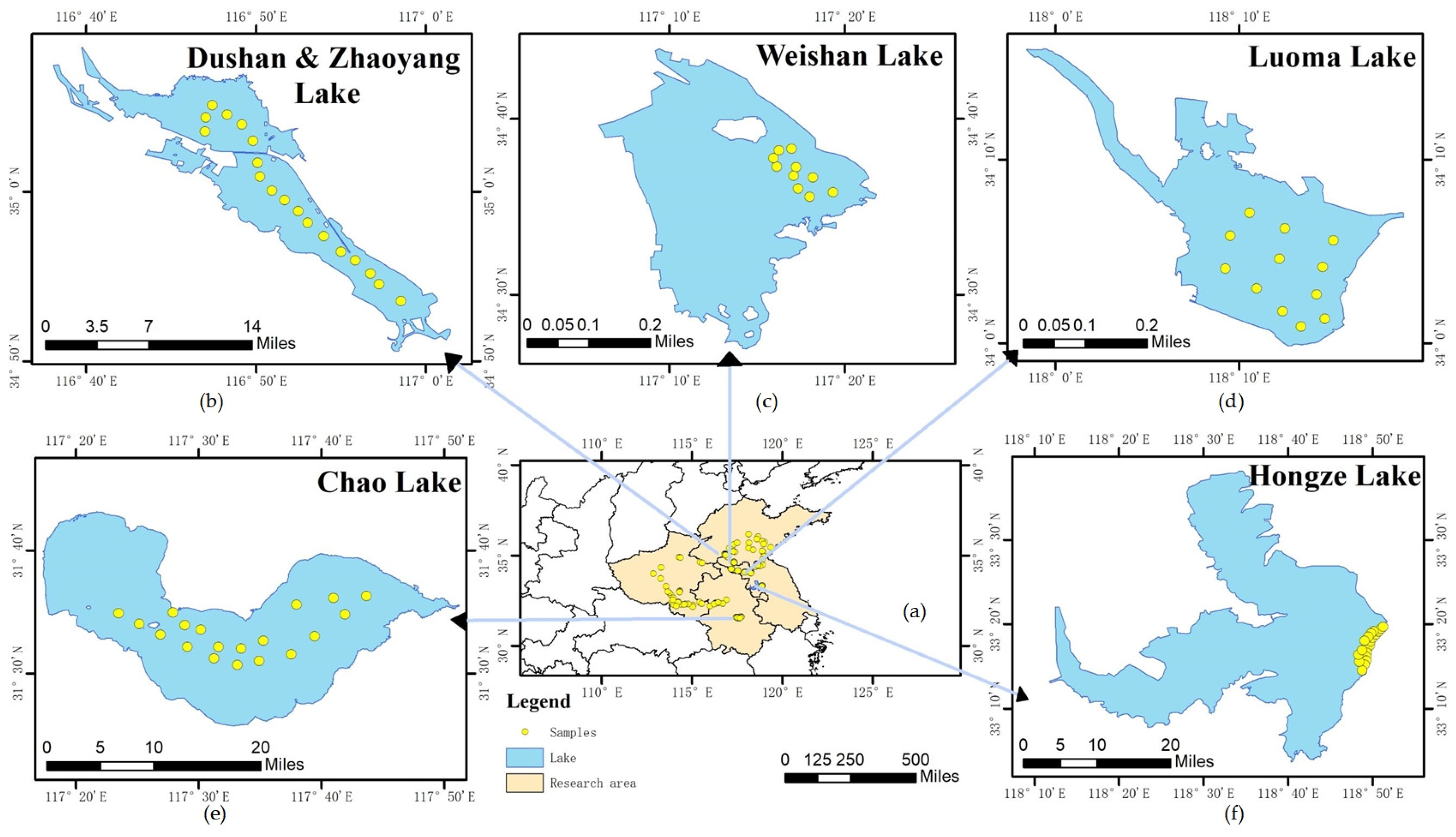
2.1. Study Area

As shown in Figure 1, we have conducted extensive field data collection in multiple representative lake, reservoir, and river regions across China in this study, encompassing areas such as Hongze Lake, Chaohu Lake, Luoma Lake, Zhaoyang Lake, Weishan Lake, Dushan Lake, and the Huai River Basin, among others. Several reservoirs with typical significance were also selected for in-depth research purposes. The geographical locations of these sites span a wide range of latitudes and longitudes, from 119.33°E to 112.83°E and 36.17°N to 31.51°N, ensuring diverse spatial distribution.

Key data collected include hyperspectral measured remote sensing reflectance, particulate matter absorption coefficients, and non-pigment particulate matter absorption coefficients, which provide a wealth of material for an in-depth investigation into the optical characteristics and water quality properties of various water bodies.

The chosen study areas not only exhibit significant differences in optical properties but also display broad representativeness in terms of water quality attributes and geographic spatial configurations. This satisfies the stringent requirements for sample diversity in constructing classification and regression models.

2.2. In Situ Data Collection

At each sampling point across the aforementioned study regions, simultaneous measurements were taken for parameters including hyperspectral in situ remote sensing reflectance, particulate matter absorption coefficients, and non-pigment particulate matter absorption coefficients. The data collection period spanned from 6 July 2021 to 24 February 2023, resulting in a total of 160 sets of sample data.

Remote sensing reflectance spectral resolution (R_rs) at wavelength λ was determined using a Field Spec Pro FR instrument (ASD Inc., Longmont, CO, USA), which operates across the 350–1050 nm range, with data resolution refined to 1 nm by internal software. Measurements adhered to NASA Ocean Optics protocols, where the device was manually held above the water surface approximately 1 m from an anchored ship’s deck. Both the water surface radiance (L_sw) and the radiance of a standard gray board (L_p) were quantified, acquiring ten spectra for each target. The instrument orientation had a viewing angle φ_v set between 90 and 135°, ensuring the plane of incident radiation was not sun-facing. The observation direction of the water surface was maintained within a 30–45° angle, thereby minimizing direct sunlight influence and reducing interference from the ship’s shadow. After capturing water radiance, the spectro-radiometer was rotated upward by 90–120° to measure sky radiance (L_sky). Here, the view zenith angle matched that used during water radiance measurement. Hyperspectral reflectance calculation followed Equation (1):

$$R_{rs}=\left(L_{sw}-r{L}_{sky}\right)/(L_p\times \pi /{\rho }_p)$$

(1)

where ${\rho }_p$ is the reflectance of the gray board, and r represents the reflectance of the skylight at the air–water interface.

Pigments were derived using 90% ethanol heated to 80 °C, and the chlorophyll a (Chla) concentration was quantified through fluorimetric assays as per Welschmeyer’s method [36]. The gravimetric determination technique, as detailed by Zhang et al. [37], was employed to ascertain the concentrations of total suspended matter (TSM), organic suspended matter (OSM), and inorganic suspended matter (ISM). This process involved passing samples through pre-combusted Whatman GF/F filters with 0.70 μm pores that had been treated at 550 °C for four hours to eliminate residual organic material on the filter membrane. Post-filtration, the filters were dried at 105 °C for four hours to calculate TSM weights. Subsequently, the filters underwent re-combustion at 550 °C for another four-hour period, followed by re-weighing to derive ISM values. OSM concentrations were calculated as the difference between TSM and ISM.

Water component absorption spectra were measured in the laboratory utilizing quantitative filtration technology (QFT), which entailed determining the absorption coefficients for total particulate matter (a_p(λ)) and non-phytoplankton particulates (a_nap(λ)). These absorption spectra were captured at 1 nm intervals from 350 to 800 nm using a Shimadzu UV-2550 PC UV-Vis spectrophotometer. To isolate the absorption coefficient for phytoplankton particles (a_ph(λ)), a_nap(λ) was subtracted from a_p(λ), following Equation (2).

$$a_{ph}\left(\lambda \right)=a_p\left(\lambda \right)-a_{nap}\left(\lambda \right)$$

(2)

In addition, water samples were initially filtered through a 47 mm diameter Whatman fiberglass GF/F filter with 0.70 μm pore size, and then subjected to secondary filtration using a 25 mm diameter Millipore filter with a 0.22 μm pore size to obtain CDOM absorption spectra (a_CDOM(λ)).

2.3. A Novel Two-Stage Framework for a_ph(λ) Inversion Combining Optical Classification and Regression

The framework comprises two stages (Figure 2): optical classification and regression inversion. First, hyperspectral reflectance data undergo Kernel Principal Angle-based Component (KPAC) dimensionality reduction and Chameleon Swarm Algorithm (CSA)-optimized k-medoids clustering to categorize water bodies into four optical classes. Second, L1-norm feature-selected XGBoost models are trained for each class to invert (a_ph(λ) parameters. The optical classification stage groups water bodies into distinct spectral types (C1–C4), while the regression stage leverages these class-specific spectral features to optimize the inversion of a_ph(λ) parameters. This hierarchical approach ensures model adaptability to diverse optical conditions.

For the optical clustering framework, the input data include R_rs and parameters of the k-medoids algorithm (the number of clusters and the distance function). Among them, R_rs undergoes feature dimensionality reduction through KPAC analysis. The parameters of the algorithm are globally optimized by the CSA. Finally, the clustering labels (C1–C4) based on the waveform features of the reflectance are output.

For the regression modeling process, the input is 501-band hyperspectral remote sensing reflectance data, and the output target parameters are pigment particle absorption coefficients a_ph(440), a_ph(555), a_ph(675), and a_ph(709). The dataset is randomly divided into a training set (80%), a validation set (10%), and a test set (10%) according to a certain proportion to ensure the independence of model training and evaluation. The training/validation split ensures spectral diversity within each lake, though external validation across unstudied regions is recommended for future work.

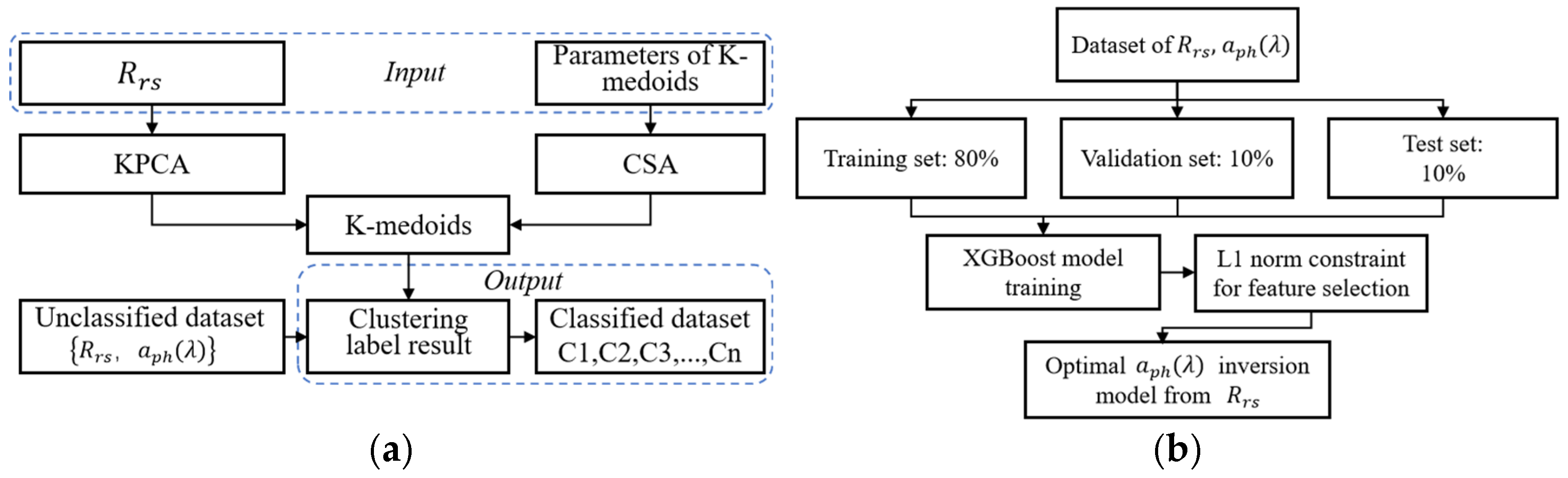
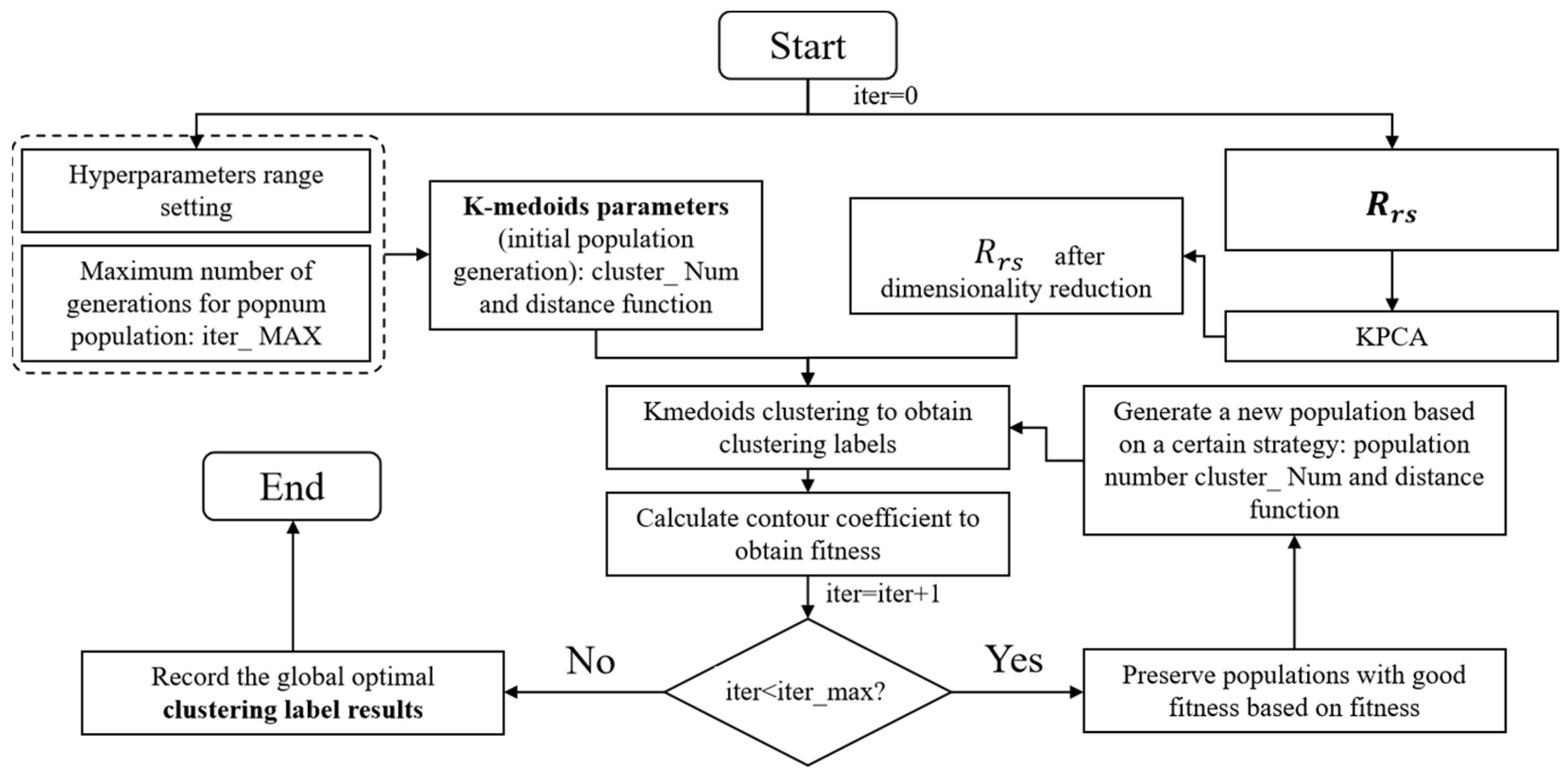
2.3.1. K-Medoid Optical Clustering Method Based on KPAC Dimensionality Reduction and CSA

Accurate characterization of effective features and their interrelationships is pivotal in high-dimensional data processing. As shown in Figure 3, this study proposes an optimized framework integrating KPCA dimensionality reduction with enhanced K-medoids clustering for 501-band hyperspectral remote sensing reflectance data. The methodology proceeds as follows:

(1)

KPAC Dimensionality Reduction:

KPAC extends Kernel PCA by incorporating angular metrics to preserve nonlinear relationships in high-dimensional spectral data. It maps input features into a higher-dimensional space using a kernel function (e.g., RBF), and then performs PCA to extract principal components based on the angles between feature vectors. This captures discriminative spectral features while reducing redundancy. The method selects components that maximize variance in the kernel space, ensuring critical absorption features (e.g., peaks at 440 nm and 675 nm) are retained for clustering.

(2)

CSA Optimization for k-medoids:

CSA optimizes k-medoids hyperparameters (cluster number k and distance metric) by simulating chameleon foraging behavior. The algorithm iteratively updates solutions via three phases:

Prey Search: Explores the parameter space using adaptive step sizes.

Eye Rotation: Adjusts search direction based on local and global best solutions.

Prey Capture: Converges to the optimal solution by minimizing the silhouette coefficient (fitness function).

The process terminates when the maximum iterations (iter_MAX) are reached or the fitness stabilizes.

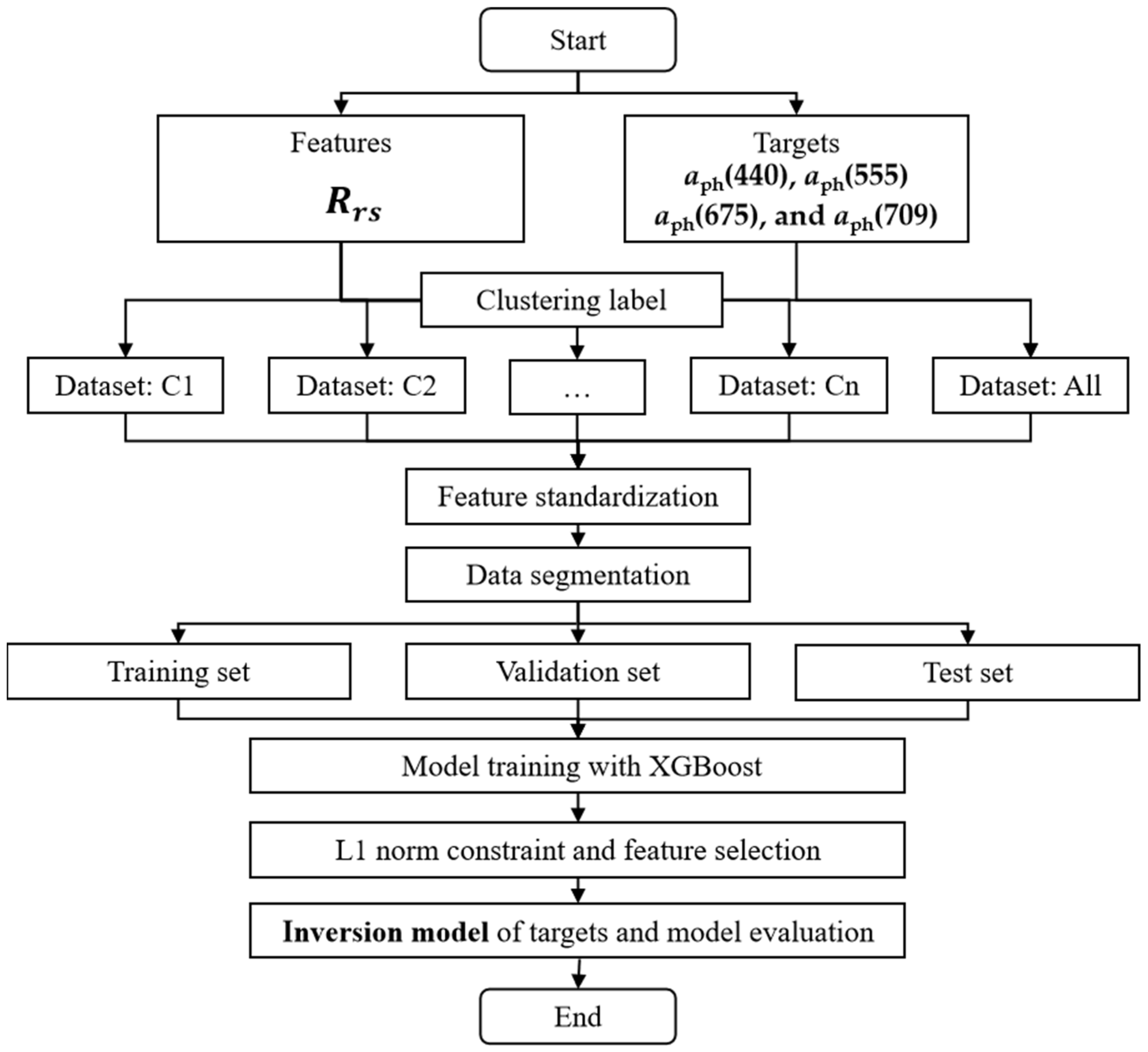
2.3.2. XGBoost Regression Method Based on L1-Norm Feature Selection

As shown in Figure 4, this study employs the XGBoost regression method based on L1-norm feature selection to identify the characteristic bands that can accurately inverse the absorption coefficients of four pigment particles, namely a_ph(440), a_ph(555), a_ph(675), and a_ph(709). L1-norm optimizes dimensionality reduction and overfitting suppression via sparse feature weighting. The procedure is illustrated in the figure below:

(1)

Data Preparation and Normalization: Construct datasets integrating full-band reflectance spectra with target parameters, followed by feature standardization to mitigate scale variance.

(2)

Regularized Model Training: Partition data into training (80%), validation (10%), and test sets (10%). Implement L1-norm constraints within the loss function to enforce feature sparsity during XGBoost training.

(3)

Spectral Band Selection: Eliminate non-informative bands exhibiting zero feature weights post-regularization, establishing a parsimonious inversion model.

(4)

Accuracy Validation: Quantify model performance using root mean square error (RMSE) and coefficient of determination (R²) metrics on independent test data.

While not explicitly modeled, fluorescence signatures are inherently captured in the reflectance spectra and contribute to the empirical relationships learned by the regression algorithm.

3. Results

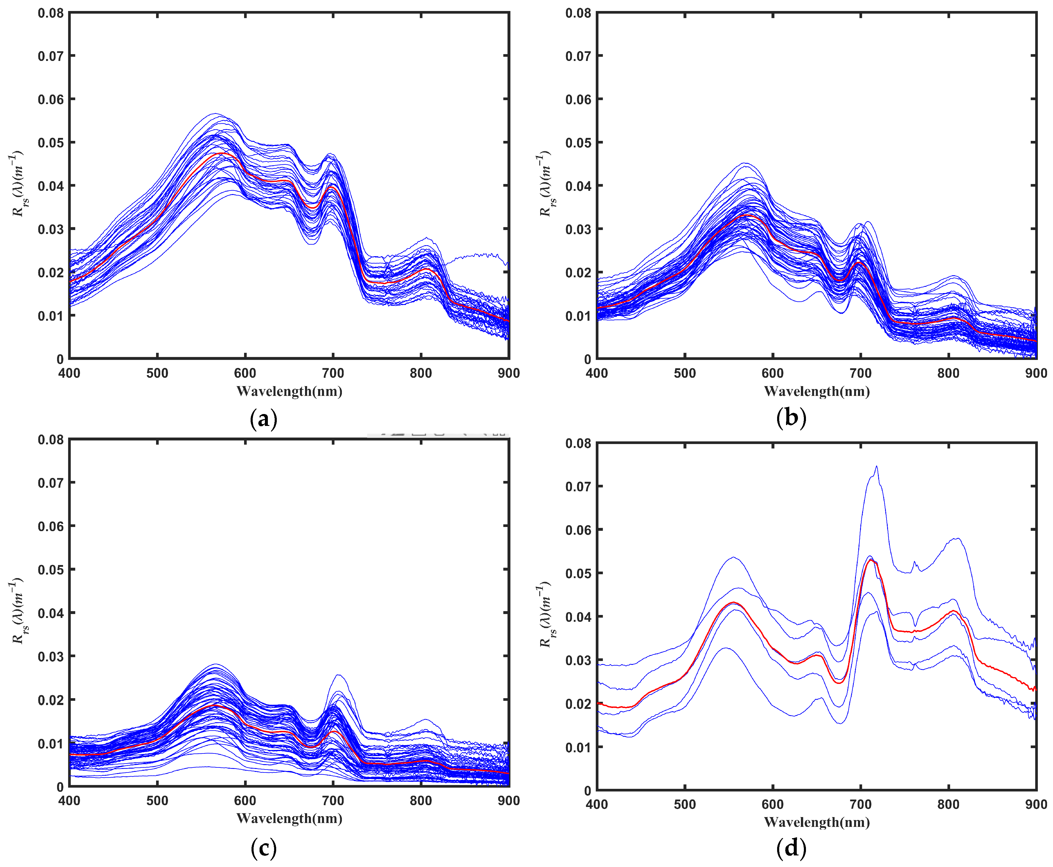
3.1. Spectrum of Remote Sensing Reflectance and Pigment Particle Absorption Coefficient

The absorption coefficient of planktonic plants varies with the wavelength of light. Two local maximum values can be observed near the wavelengths of 440 nm and 675 nm, while two local minimum values can be seen near the wavelengths of 555 nm and 709 nm. These absorption coefficient curves can be used to characterize the characteristics of pigment particle absorption coefficients.

In Figure 5a, the y-axis is the remote sensing reflectance and the x-axis is the center wavelength value of the spectral channel bands. According to the data in Figure 5a, we can summarize the spectral characteristics as follows: there are peaks in the wavelength ranges of 550–580 nm, 700 nm, and 820 nm. In the wavelength range of 390 nm to 580 nm, the remote sensing reflectance exhibits a monotonically increasing trend. However, in the wavelength range of 580 nm to 600 nm, the remote sensing reflectance decreases drastically. In the wavelength range of 600 nm to 660 nm, the remote sensing reflectance changes relatively smoothly. In the wavelength range of 660–700 nm, there is a small reflection valley at 680 nm. At 700 nm, the remote sensing reflectance reaches its peak, then decreases abruptly at 720 nm. In the wavelength range of 800 nm, the remote sensing reflectance reaches its peak again, followed by a gradual decrease and tendency towards stability. It should be noted that the maximum value is not always at 580 nm. In some cases, the reflection rate may be higher at 700 nm.

In Figure 5b, the y-axis is the absorption coefficient of pigment particles, and the x-axis is the center wavelength value of the spectral channel bands. The absorption coefficient of pigment particles is the difference between the total particle absorption coefficient and the absorption coefficient of non-pigment particles, which is expressed as a_ph(λ) = a_p(λ) − a_d(λ). The absorption coefficient of planktonic plants exhibits a variable pattern with the wavelength of light. Near the wavelengths of 440 nm and 675 nm, two local maximum values can be observed, while two local minimum values emerge near the wavelengths of 555 nm and 709 nm. The absorption coefficient curves provide a comprehensive characterization of the absorption characteristics of pigment particles. The curve demonstrates a sudden increase in the absorption coefficient between 390 and 440 nm, followed by a rapid decrease from 440 nm to 555 nm. Afterward, the coefficient experiences a slight peak at 630 nm and a slight trough at 650 nm before reaching a larger peak at 700 nm. Finally, the absorption coefficient drops to zero at 709 nm and remains constant thereafter. The 709 nm wavelength is emphasized due to its established role in pigment absorption spectra, even though local minima may shift slightly depending on water composition (see Figure 5b).

3.2. Result of Classification

The remote sensing reflectance spectrum of each water classification is shown in Figure 6. Although different types of waters generally have low reflectance and gradually decreasing reflectance from red to near-infrared bands, approaching zero, the varying components of these waters result in significant differences in their reflectance waveform characteristics. Although all R_rs values have reflection peaks near 550 nm, 650 nm, 700 nm, and 800 nm, the steepness of each OWT is distinct. The common characteristic of Class 1 (C1), Class 2 (C2), and Class 3 (C3) in the visible light band is that their reflection peak at 550 nm is higher than those at 650 nm, 700 nm, and 800 nm, with a relatively smaller spectral amplitude in the near-infrared band. The peak at 550 nm may be attributed to the weak absorption of chlorophyll a and carotene, as well as the enhancement of particle scattering caused by biological sources (such as phytoplankton) and abiotic sources (such as sediments) [38,39]. While magnitude differences are visually prominent in the composite spectra (Figure 5), the KPAC-CSA clustering effectively captures both magnitude and subtle shape features through nonlinear dimensionality reduction and DTW distance metrics [23,35]. The four distinct optical classes identified by this approach are characterized as follows:

C1 waters exhibit smooth average R_rs spectra in the visible light band, with overall large remote sensing reflectance amplitude. This is due to strong scattering associated with sediments, which masks the spectral fluctuations caused by water component absorption [40]. The remote sensing reflectance decreases relatively gently within the 555 nm to 700 nm range, and the slope of the decrease becomes steeper from 700 nm to 740 nm. A relatively large reflection peak occurs at 800 nm.

C2 waters have median remote sensing reflectance values, with a gradual decrease in remote sensing reflectance after 550 nm, and a large overall descent slope.

C3 waters exhibit the smallest overall remote sensing reflectance.

Class 4 (C4) waters: Among the four types of waters, they have the largest amplitude and frequency of remote sensing reflectance variation with wavelength, with their maximum reflection peak at 720 nm. The remote sensing reflectance amplitude is large within the 720 nm to 900 nm range, differing significantly from the other three classes.

Figure 7 shows the absorption coefficient of pigment particles spectrum of each water classification. Although the differences in the remote sensing reflectance spectra of different water classifications in Figure 5 are relatively obvious, the differences in the spectra of pigment particle absorption coefficients of various water types in Figure 6 are not very prominent.

The spectra of water types C1 and C2 have similar overall trends. However, the decrease in a_ph(λ) in the 440–450 nm range of C2 is gentler. In addition, C1, C2, and C3 all show an upward trend in the 555–650 nm range.

Among all the water classifications, C3 exhibits the most distinct characteristics. In the wavelength range of 380–440 nm, while the a_ph(λ) of other water types shows an overall upward trend, the a_ph(λ) of C3 remains flat in this range, with a value basically around 1. In the 555–650 nm range, C3 also shows a flat trend.

C4 has unique features. In the range of 380–440 nm, the a_ph(λ) not only shows an overall upward trend but also presents a flat platform state between 420 and 440 nm, and its overall values are relatively large.

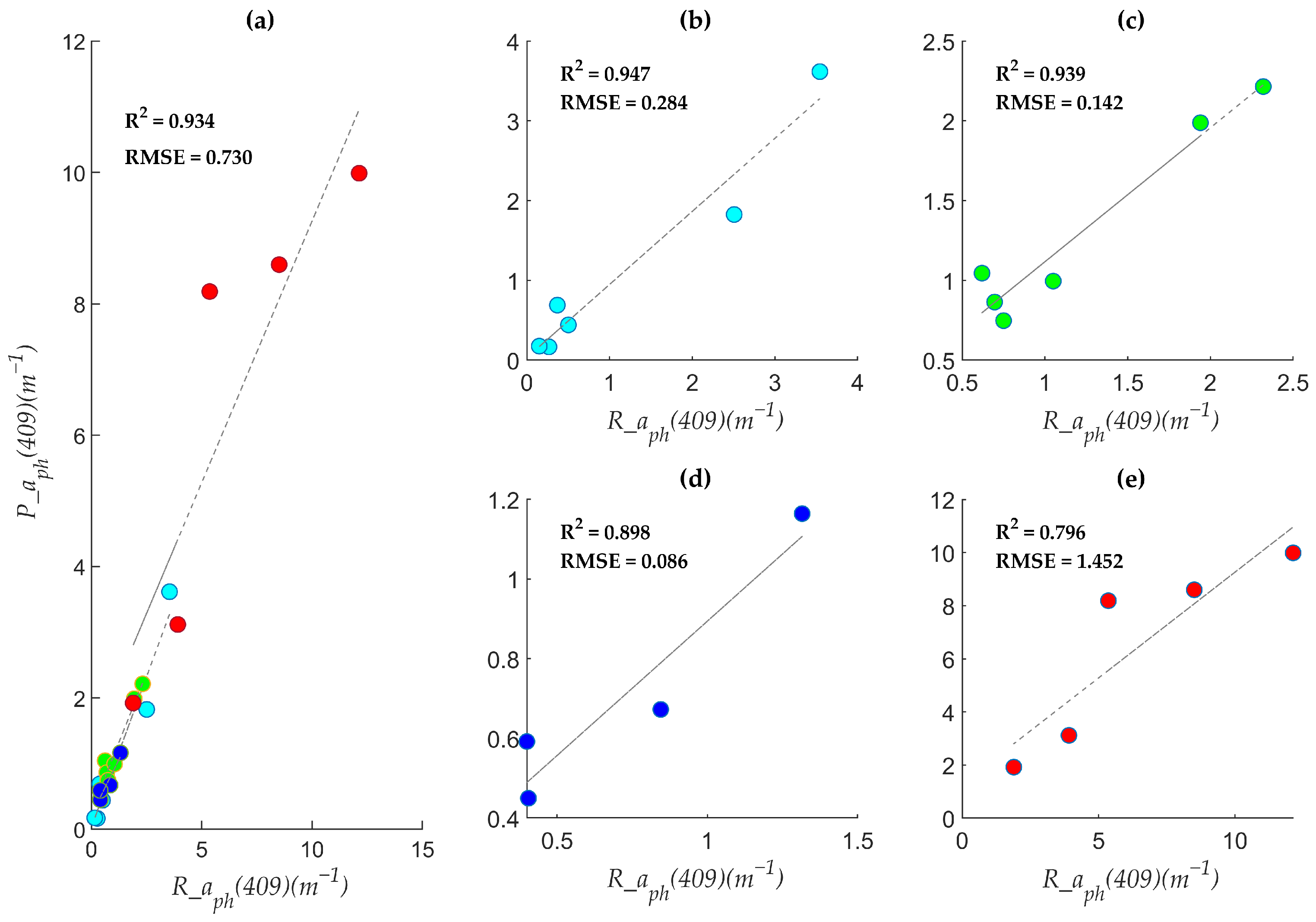
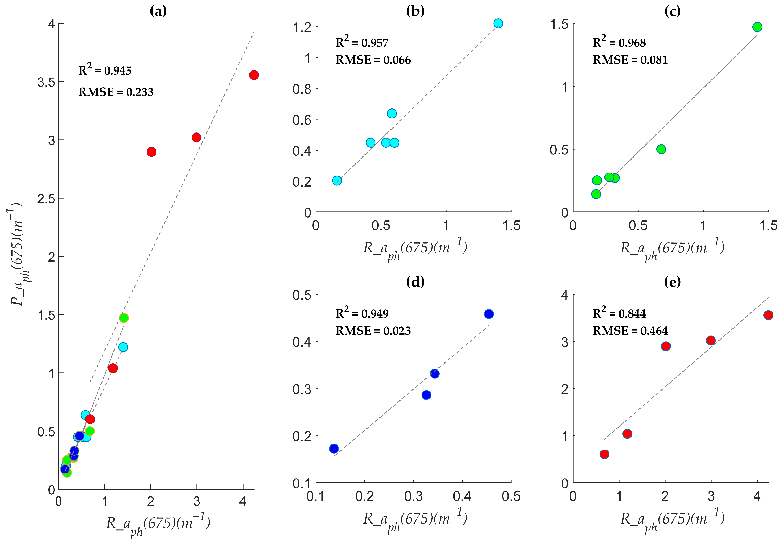
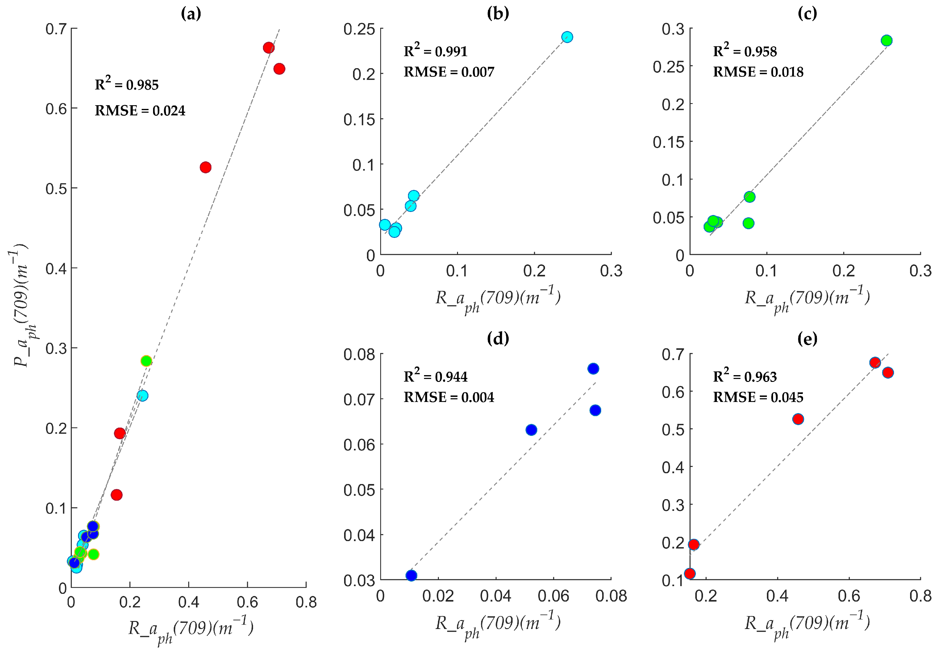
3.3. Result of Regression

Table 1. Model fitting results of a_ph(440), a_ph(555), a_ph(675), and a_ph(709) under different water classifications.

Parameters	Clusters	RMSE	R2	λ (nm)
aph(440)	Unclassified dataset	2.07	0.457	761,762,899
	C1	0.284	0.947	677,711,734
	C2	0.142	0.939	443,719,729
	C3	0.086	0.898	438,677,714
	C4	1.452	0.796
	Pooled C1–C4	0.730	0.934	/
aph(555)	Unclassified dataset	0.09	0.822	441,676,677,714,715,735
	C1	0.007	0.998	500,730,734
	C2	0.042	0.948	441,628,728,729
	C3	0.017	0.891	415,717,721
	C4	0.183	0.877
	Pooled C1–C4	0.092	0.961	/
aph(675)	Unclassified dataset	0.40	0.714	441,677,735,739,748
	C1	0.066	0.957	727,730
	C2	0.081	0.968	441,548,627,681,715
	C3	0.023	0.949	549,679,721
	C4	0.464	0.844
	Pooled C1–C4	0.233	0.945	/
aph(709)	Unclassified dataset	0.35	0.749	441,677,714,715,748
	C1	0.007	0.991	494,729,734
	C2	0.018	0.958	441,680,681,719,728
	C3	0.004	0.944	720
	C4	0.045	0.963
	Pooled C1–C4	0.024	0.985	/

presents the model fitting results of a_ph(440), a_ph(555), a_ph(675), and a_ph(709) under different water classifications. The unclassified scenario represents traditional inversion approaches that directly fit models on the entire dataset without optical classification. In contrast, our classification-based method groups waters into four optical types (C1–C4) and achieves significant improvements in both R² and RMSE, as shown in Table 1.

Figure 8, Figure 9, Figure 10 and Figure 11 illustrate the relationship between the measured raw a_ph(λ) and the predicted a_ph(λ), specifically, C1, C2, C3, and C4, and pooled C1–C4 in general. Due to the small sample size of C4 (only five sample points), no data segmentation was carried out, and linear fitting was directly applied.

For a_ph(440), compared with the unclassified dataset, the R² of the pooled dataset of C1–C4 (pooled C1–C4) increased significantly from 0.457 to 0.934, and the RMSE decreased substantially from 2.07 to 0.730, representing a decrease of approximately 64.7%. Among the various classifications, the R² values of C1 and C2 were both higher than 0.93, demonstrating relatively excellent performance; the R² of C3 was 0.898, showing acceptable performance; and the R² of C4 was only 0.796, indicating relatively poor performance. Overall, the classification significantly improved the model accuracy.

For a_ph(555), the R² of the unclassified dataset was 0.822, and that of the pooled dataset of C1–C4 increased to 0.961. Among them, the R² of C1 was as high as 0.998, showing the best performance; the R² values of C2 and C3 were 0.948 and 0.891, respectively. Although lower than that of C1, they still enhanced the performance of the pooled dataset of C1–C4 as a whole. Compared with the R² increase amplitudes of a_ph(440), a_ph(675), and a_ph(709) after classification, the increase amplitude of a_ph(555) was relatively small, and the RMSE changed slightly. Nevertheless, the overall model performance was still optimized to some extent after classification.

For a_ph(675), the R² of the unclassified dataset was 0.714, and the RMSE was 0.40. The R² of the pooled dataset of C1–C4 increased to 0.945, and the RMSE decreased to 0.233, a decrease of approximately 41.7%. Among the four classifications, the R² of C2 was the highest, reaching 0.968; the RMSE of C3 was the lowest, only 0.023, indicating high prediction accuracy; the R² of C4 was 0.844, and the RMSE was 0.464, showing relatively poor performance compared with the other three classifications. Compared with a_ph(440) and a_ph(555), the improvement degree of a_ph(675) after classification was at a medium level, and classification significantly improved its inversion accuracy.

For a_ph(709), the R² of the unclassified dataset was 0.749, and the RMSE was 0.35. The R² of the pooled dataset of C1–C4 increased significantly to 0.985, and the RMSE decreased to 0.024, with the RMSE decreasing by approximately 93.1%. The R² of C1 was 0.991, and the RMSE was 0.007, showing the most outstanding performance; the R² values of C2, C3, and C4 were also all higher than 0.94, indicating a significant classification effect. Among the four parameters, the improvement amplitude of a_ph(709) after classification was the most prominent, with the most significant effect.

Overall, water body classification improved the inversion accuracy of a_ph(440), a_ph(555), a_ph(675), and a_ph(709). Compared with the unclassified situation, classification comprehensively optimized the R² and RMSE indicators. In the C1–C4 classifications, different classifications had their respective advantages in different parameters. For example, C1 had outstanding R² performance in multiple parameters; C3 had excellent RMSE performance in some parameters. Although the R² increase amplitude of a_ph(555) after classification was relatively small, the RMSE changed slightly, and the data distribution was more reasonable. Overall, the classification algorithm demonstrated unique advantages in improving model accuracy and optimizing data distribution. While the C4 water class represents an important optical category in our dataset, its small sample size (n = 5) may affect the stability of the corresponding regression model. However, the consistent performance across wavelengths (R² = 0.796–0.963) suggests that these results remain meaningful for characterizing this water type.

4. Discussion

This study aims to accurately determine the pigment particle absorption coefficient, a crucial water–environmental parameter. Innovatively, an intelligent k-medoids clustering method, which combines KPAC dimensionality reduction and CSA optimization, is proposed for optical classification. An XGBoost regression model with L1-norm feature selection is employed for inversion. Experimental results demonstrate the effectiveness of this method: after conducting four-class optical classification on samples from lakes, reservoirs, and rivers in various regions of China, the inversion accuracy of a_ph(440), a_ph(675), and a_ph(709) is significantly improved, with R² exceeding 0.9 and RMSE being substantially reduced.

The improved accuracy of a_ph(λ) retrieval has direct implications for water quality monitoring and management. For example, more precise estimates of phytoplankton absorption coefficients can enhance the assessment of algal biomass and primary productivity [2], support eutrophication monitoring [7], and improve the parameterization of bio-optical models for light propagation in water [5]. This is particularly relevant for inland and coastal waters, where optical complexity often challenges traditional remote sensing approaches.

The differences in inversion accuracy across water classes (e.g., higher R² for a_ph(440) in C1/C2 versus lower performance for a_ph(555) in C4) align with their distinct optical features (Figure 6 and Figure 7). For instance, C1’s smooth reflectance spectra and strong scattering (Section 3.2) likely stabilize the signal for shorter wavelengths (440 nm), while C4’s pronounced 720 nm peak and high reflectance variability may introduce noise for intermediate wavelengths (555 nm). These class-specific spectral signatures, driven by varying phytoplankton and non-algal particle dominance, directly influence the regression model’s ability to isolate target parameters.

First, by analyzing the variation in pigment particle absorption coefficient at different wavelengths, we successfully revealed the importance of peaks at 440 nm and 675 nm and valleys at 555 nm and 709 nm for characterizing spectral absorption characteristics, which is consistent with what is concerned in references [9,11,12,13,24]. However, although the inversion effect is good for most parameters, compared with other parameters, the improvement in the accuracy of a_ph(555) is slightly insufficient. This may be related to the large influence of non-biological factors on light absorption at this specific wavelength or the incomplete differentiation of different types of water environments in the optical classification at this wavelength [34]. Therefore, in future research, further exploration is needed into the variation mechanism of a_ph(555) under specific environmental conditions and its intrinsic relationship with other optical parameters.

Second, the intelligent clustering method breaks through the limitations of traditional classification methods, improving the objectivity and accuracy of classification. The XGBoost regression model can automatically select feature bands with high correlations, reduce the influence of irrelevant variables, and enhance the inversion performance, providing new ideas for the remote sensing monitoring research of the absorption characteristics of pigment particles in water bodies.

Although this study has achieved remarkable results, there is still room for improvement. For example, the sample size can be expanded to cover more types of water environments, and data collection on seasonal and regional variations can be increased to test the universality and stability of the model. Future studies could further strengthen these findings by incorporating additional C4-type samples and applying cross-validation techniques to verify model stability across similar optical water types. Future research will focus on the following directions: First, optimize the optical classification by incorporating the comprehensive waveform characteristics of a_ph(λ) at different wavelengths into the criteria, and study its impact on the inversion of a_ph(λ) parameters. Second, attach importance to data preprocessing, strengthen data cleaning, eliminate outliers and missing values, correct errors, balance the sample distribution, and explore advanced feature extraction and dimensionality reduction methods. Third, expand the training dataset to enhance the model’s adaptability to complex environments. While the model achieves high accuracy in the tested lakes, further validation with independent datasets from geographically distinct water bodies would help assess its broader applicability. Fourth, draw on the fine-tuning concept of LLM (Large Language Model) to construct a specific task adjustment model, LORA (Low-Rank Adaptation). By combining large models with LORA models, the performance and reliability of remote sensing monitoring and inversion of the absorption coefficients of pigment particles in water bodies can be improved.

5. Conclusions

This study developed an innovative two-stage framework combining KPAC-CSA optimized k-medoids clustering and L1-norm XGBoost regression to accurately retrieve pigment absorption coefficients (a_ph(λ)) across four key wavelengths. Our key findings demonstrate the following:

(1)

Optical classification significantly improved inversion accuracy, with R² > 0.9 for a_ph(440), a_ph(675), and a_ph(709) across water types.

(2)

The method effectively addresses current limitations in remote monitoring of pigment absorption, particularly in complex inland waters.

(3)

While performance for a_ph(555) was comparatively lower (R² = 0.877–0.998), the overall framework shows strong potential for water quality monitoring applications.

Future work should focus on the following: (1) expanding the dataset for rare water types (e.g., C4), (2) incorporating water quality parameters to enhance a_ph(555) retrieval, and (3) developing adaptive strategies for extreme conditions. This approach advances the precision of aquatic remote sensing and supports more accurate ecological assessments.

References

1. Smetacek, V.; Zingone, A. Green and golden seaweed tides on the rise. Nature 2013, 504, 84–88. [Google Scholar] [CrossRef] [PubMed]
2. Field, C.B.; Behrenfeld, M.J.; Randerson, J.T.; Falkowski, P. Primary production of the biosphere: Integrating terrestrial and oceanic components. Science 1998, 281, 237–240. [Google Scholar] [CrossRef]
3. Sosik, H.M.; Mitchell, B.G. Light absorption by phytoplankton, photosynthetic pigments and detritus in the california current system. Deep Sea Res. Part I Oceanogr. Res. Pap. 1995, 42, 1717–1748. [Google Scholar] [CrossRef]
4. Woźniak, S.B.; Litwicka, D.; Stoń-Egiert, J. Variability and relationships between particle sizes, composition and optical properties of suspended particulate matter in the coastal waters of western spitsbergen, assessed through measurements of size-fractionated seawater samples. Oceanologia 2024, 66, 66403. [Google Scholar] [CrossRef]
5. Lednicka, B.; Kubacka, M.; Freda, W.; Haule, K.; Ficek, D.; Sokólski, M. Multi-parameter algorithms of remote sensing reflectance, absorption and backscattering for coastal waters of the southern baltic sea applied to pomeranian lakes. Water 2023, 15, 2843. [Google Scholar] [CrossRef]
6. Niu, C.; Tan, K.; Wang, X.; Du, P.; Pan, C. A semi-analytical approach for estimating inland water inherent optical properties and chlorophyll a using airborne hyperspectral imagery. Int. J. Appl. Earth Obs. Geoinf. 2024, 128, 103774. [Google Scholar] [CrossRef]
7. García-Chicote, J.; Armengol, X.; Rojo, C. Zooplankton abundance: A neglected key element in the evaluation of reservoir water quality. Limnologica 2018, 69, 46–54. [Google Scholar] [CrossRef]
8. Efimova, T.; Churilova, T.; Skorokhod, E.; Suslin, V.; Buchelnikov, A.S.; Glukhovets, D.; Khrapko, A.; Moiseeva, N. Light absorption by optically active components in the arctic region (august 2020) and the possibility of application to satellite products for water quality assessment. Remote Sens. 2023, 15, 4346. [Google Scholar] [CrossRef]
9. Jiang, G.; Duan, G.; Huang, Z.; Cai, W.; Lu, C.; Su, W.; Yang, J.; Zhang, C. Remote sensing classification of the dominant optically active components and its variations in the pearl river estuary. Haiyang Xuebao 2016, 38, 64–75. [Google Scholar]
10. Matsushita, B.; Yang, W.; Yu, G.; Oyama, Y.; Yoshimura, K.; Fukushima, T. A hybrid algorithm for estimating the chlorophyll-a concentration across different trophic states in asian inland waters. ISPRS J. Photogramm. Remote Sens. 2015, 102, 28–37. [Google Scholar] [CrossRef]
11. Jiang, G.; Loiselle, S.A.; Yang, D.; Ma, R.; Su, W.; Gao, C. Remote estimation of chlorophyll a concentrations over a wide range of optical conditions based on water classification from viirs observations. Remote Sens. Environ. 2020, 241, 111735. [Google Scholar] [CrossRef]
12. Bricaud, A.; Babin, M.; Morel, A.; Claustre, H. Variability in the chlorophyll-specific absorption coefficients of natural phytoplankton: Analysis and parameterization. J. Geophys. Res. Ocean. 1995, 100, 13321–13332. [Google Scholar] [CrossRef]
13. Xu, J.; Lei, S.; Bi, S.; Li, Y.; Lyu, H.; Xu, J.; Xu, X.; Mu, M.; Miao, S.; Zeng, S.; et al. Tracking spatio-temporal dynamics of poc sources in eutrophic lakes by remote sensing. Water Res. 2020, 168, 115162. [Google Scholar] [CrossRef]
14. Hu, L.; Liu, Z. Deriving absorption coefficients from remote sensing reflectance using the quasi analytical algorithm (qaa) in the yellow sea. Period. Ocean. Univ. China 2007, S2, 7. [Google Scholar]
15. Lee, Z.; Carder, K.L.; Arnone, R.A. Deriving inherent optical properties from water color: A multiband quasi-analytical algorithm for optically deep waters. Appl. Opt. 2002, 41, 5755. [Google Scholar] [CrossRef] [PubMed]
16. Yang, W.; Matsushita, B.; Chen, J.; Yoshimura, K.; Fukushima, T. Application of a semianalytical algorithm to remotely estimate diffuse attenuation coefficient in turbid inland waters. IEEE Geosci. Remote Sens. Lett. 2014, 11, 1046–1050. [Google Scholar] [CrossRef]
17. Zhan, J.; Zhang, D.J.; Zhang, G.Y.; Wang, C.X.; Zhou, G.Q. Estimation of optical properties using qaa-v6 model based on modis data. Int. Arch. Photogramm. Remote Sens. Spat. Inf. Sci. 2020, XLII-3/W10, 937–940. [Google Scholar] [CrossRef]
18. Lee, Z.; Weidemann, A.; Kindle, J.; Arnone, R.; Carder, K.L.; Davis, C. Euphotic zone depth: Its derivation and implication to ocean-color remote sensing. J. Geophys. Res. Ocean. 2007, 112, 2006JC003802. [Google Scholar] [CrossRef]
19. Yang, W.; Matsushita, B.; Chen, J.; Yoshimura, K.; Fukushima, T. Retrieval of inherent optical properties for turbid inland waters from remote-sensing reflectance. IEEE Trans. Geosci. Remote Sens. 2013, 51, 3761–3773. [Google Scholar] [CrossRef]
20. Robert Chen, F.; Lee, Z.; Carder, K.L. An bathymetric algorithm of water-leaving radiances in aviris imagery: Use of a reflectance model. In Space Remote Sensing of Subtropical Oceans (SRSSO); COSPAR Colloquia Series; COSPAR: Paris, France, 1997; pp. 221–228. Available online: https://linkinghub.elsevier.com/retrieve/pii/S0964274997800261 (accessed on 31 January 2024). [CrossRef]
21. Zibordi, G.; Berthon, J.F.; Talone, M.; Gossn, J.I.; Dessailly, D.; Kwiatkowska, E. Assessment of olci-a derived aquatic optical properties across european seas. IEEE Geosci. Remote Sens. Lett. 2023, 20, 1502605. [Google Scholar] [CrossRef]
22. Zhang, Y.; Shen, F.; Zhao, H.; Sun, X.; Zhu, Q.; Li, M. Optical distinguishability of phytoplankton species and its implications for hyperspectral remote sensing discrimination potential. J. Sea Res. 2024, 202, 102540. [Google Scholar] [CrossRef]
23. Li, Y.; Zhao, H.; Bi, S.; Lyu, H. Research progress of remote sensing monitoring of case ii water environmental parameters based on water optical classification. Natl. Remote Sens. Bull. 2021, 26, 19–31. [Google Scholar] [CrossRef]
24. Le, C.; Li, Y.; Zha, Y.; Sun, D. Specific absorption coefficient and the phytoplankton package effect in lake taihu, china. Hydrobiologia 2009, 619, 27–37. [Google Scholar] [CrossRef]
25. Spyrakos, E.; O’donnell, R.; Hunter, P.D.; Miller, C.; Scott, M.; Simis, S.G.; Neil, C.; Barbosa, C.C.; Binding, C.E.; Bradt, S.; et al. Optical types of inland and coastal waters. Limnol. Oceanogr. 2018, 63, 846–870. [Google Scholar] [CrossRef]
26. Arst, H.; Reinart, A. Application of optical classifications to north european lakes. Aquat. Ecol. 2009, 43, 789–801. [Google Scholar] [CrossRef]
27. D’Alimonte, D.; Zibordi, G.; Berthon, J.-F. A statistical index of bio-optical seawater types. IEEE Trans. Geosci. Remote Sens. 2007, 45, 2644–2651. [Google Scholar] [CrossRef]
28. Koenings, J.P.; Edmundson, J.A. Secchi disk and photometer estimates of light regimes in alaskan lakes: Effects of yellow color and turbidity. Limnol. Oceanogr. 1991, 36, 91–105. [Google Scholar] [CrossRef]
29. Koponen, S. Lake water quality classification with airborne hyperspectral spectrometer and simulated meris data. Remote Sens. Environ. 2002, 79, 51–59. [Google Scholar] [CrossRef]
30. Reinart, A.; Herlevi, A.; Arst, H.; Sipelgas, L. Preliminary optical classification of lakes and coastal waters in estonia and south finland. J. Sea Res. 2003, 49, 357–366. [Google Scholar] [CrossRef]
31. Zhang, Y.; Zhang, B.; Ma, R.; Feng, S.; Le, C. Optically active substances and their contributions to the underwater light climate in lake taihu, a large shallow lake in china. Fundam. Appl. Limnol. 2007, 170, 11–19. [Google Scholar] [CrossRef]
32. Li, Y.; Wang, Q.; Wu, C.; Zhao, S.; Xu, X.; Wang, Y.; Huang, C. Estimation of chlorophyll a concentration using nir/red bands of meris and classification procedure in inland turbid water. IEEE Trans. Geosci. Remote Sens. 2012, 50, 988–997. [Google Scholar] [CrossRef]
33. Xi, H.; Hieronymi, M.; Röttgers, R.; Krasemann, H.; Qiu, Z. Hyperspectral differentiation of phytoplankton taxonomic groups: A comparison between using remote sensing reflectance and absorption spectra. Remote Sens. 2015, 7, 14781–14805. [Google Scholar] [CrossRef]
34. Prieur, L.; Sathyendranath, S. An optical classification of coastal and oceanic waters based on the specific spectral absorption curves of phytoplankton pigments, dissolved organic matter, and other particulate materials1. Limnol. Oceanogr. 1981, 26, 671–689. [Google Scholar] [CrossRef]
35. Zhou, B.; Zhang, Y.; Shi, K. Research progress on remote sensing assessment of lake nutrient status and retrieval algorithms of characteristic parameters. Natl. Remote Sens. Bull. 2022, 26, 77–91. [Google Scholar] [CrossRef]
36. Welschmeyer, N.A. Fluorometric analysis of chlorophyll a in the presence of chlorophyll b and pheopigments. Limnol. Oceanogr. 1994, 39, 1985–1992. [Google Scholar] [CrossRef]
37. Zhang, Y.; Zhang, B.; Wang, X.; Li, J.; Feng, S.; Zhao, Q.; Liu, M.; Qin, B. A study of absorption characteristics of chromophoric dissolved organic matter and particles in lake taihu, china. Hydrobiologia 2007, 592, 105–120. [Google Scholar] [CrossRef]
38. Ahn, Y.-H.; Bricaud, A.; Morel, A. Light backscattering efficiency and related properties of some phytoplankters. Deep Sea Res. Part A Oceanogr. Res. Pap. 1992, 39, 1835–1855. [Google Scholar] [CrossRef]
39. Kutser, T. Quantitative detection of chlorophyll in cyanobacterial blooms by satellite remote sensing. Limnol. Ocean. 2004, 49, 2179–2189. [Google Scholar] [CrossRef]
40. Bi, S.; Li, Y.; Xu, J.; Liu, G.; Song, K.; Mu, M.; Lyu, H.; Miao, S.; Xu, J. Optical classification of inland waters based on an improved Fuzzy C-Means method. Opt. Express 2019, 27, 34838–34856. [Google Scholar] [CrossRef]
Figure 1. Study area (latitude: 31.51°N–36.17°N, longitude: 112.83°E–119.33°E): all samples (a); samples from Dushan and Zhaoyang Lake in July 2021 (b); samples from Weishan Lake in July 2021 (c); samples from Luoma Lake in November 2020 (d); samples from Chao Lake in July 2021 (e); samples from Hongze Lake in February 2023 (f).
Remotesensing 17 01756 g001
Figure 2. Two-stage framework for aph(λ) inversion: (a) optical clustering method and (b) regression.
Remotesensing 17 01756 g002
Figure 3. Flowchart of K-medoid optical clustering method.
Remotesensing 17 01756 g003
Figure 4. Flowchart of XGBoost regression method based on L1-norm feature selection.
Remotesensing 17 01756 g004
Figure 5. Spectrum of (a) Rrs(λ) and (b) aph(λ) of our dataset, n = 160.
Remotesensing 17 01756 g005
Figure 6. Remote sensing reflectance spectrum of each water classification (red lines indicating the mean values for each class): C1 (a), C2 (b), C3 (c), and C4 (d). The thin blue curves are Rrs measured in situ, and the red bold curves are the mean Rrs of each cluster.
Remotesensing 17 01756 g006
Figure 7. Absorption coefficient of pigment particles spectrum of each water classification (red lines indicating the mean values for each class): C1 (a), C2 (b), C3 (c), and C4 (d).
Remotesensing 17 01756 g007
Figure 8. The relationship between measured raw aph(440) and predicted aph(440): pooled C1–C4 (a); C1 (cyan color) (b); C2 (green color) (c); C3 (blue color) (d); and C4 (red color) (e).
Remotesensing 17 01756 g008
Figure 9. The relationship between measured raw aph(555) and predicted aph(555): pooled C1–C4 (a); C1 (cyan color) (b); C2 (green color) (c); C3 (blue color) (d); and C4 (red color) (e).
Remotesensing 17 01756 g009
Figure 10. The relationship between measured raw aph(675) and predicted aph(675): pooled C1–C4 (a); C1 (cyan color) (b); C2 (green color) (c); C3 (blue color) (d); and C4 (red color) (e).
Remotesensing 17 01756 g010
Figure 11. The relationship between measured raw aph(709) and predicted aph(709): pooled C1–C4 (a); C1 (cyan color) (b); C2 (green color) (c); C3 (blue color) (d); and C4 (red color) (e).
Remotesensing 17 01756 g011