Abstract
Accurate prediction of the spatiotemporal distribution of chlorophyll-a (Chl-a) is essential for evaluating marine ecosystem health and predicting ecological disasters. Current methods struggle to capture short-term variability and periodic trends in Chl-a, especially in noise-prone coastal regions. This study aims to enhance the prediction of marine Chl-a concentrations by introducing the chlorophyll-a concentration prediction model (ChlaPM), which was developed on the basis of a convolutional long short-term memory (ConvLSTM) network. The model integrates recent spatiotemporal feature extraction (RSTFE), periodic feature extraction (PFE), and denoising fusion (DNF) modules to effectively capture short-term spatiotemporal changes and periodic variations in Chl-a concentrations. In this study, the performance of ChlaPM in single-step and multistep predictions was evaluated using monthly average Chl-a remote sensing data spanning 1998–2023. The results indicate that compared with the RSTFE model, the ChlaPM model achieves substantial reductions in the root mean square error (RMSE) of 53.84%, 53.58%, and 49.70% for predicting Chl-a concentrations 1 month, 3 months, and 6 months into the future, respectively. These findings highlight the effectiveness of ChlaPM in addressing short-term variability and periodic trends and significantly enhances the accuracy of Chl-a prediction. Future work will focus on integrating additional relevant marine variables into the prediction model to further improve its prediction capabilities.
1. Introduction
The chlorophyll-a (Chl-a) concentration in marine phytoplankton serves as a critical indicator of oceanic primary productivity and is closely linked to the vitality and health of marine ecosystems. Fluctuations in chlorophyll-a (Chl-a) concentrations are intrinsically tied to marine ecosystem health and play a critical role in regulating the stability of marine food webs. These dynamics ultimately shape the spatial distribution and availability of fishery resources—a cornerstone of global food security [1,2,3,4]. Moreover, understanding the spatiotemporal variation in Chl-a concentrations is essential for a range of environmental applications. For example, accurate predictions can aid in monitoring dynamic ecosystem changes, assessing environmental health, and providing early warnings for ecological disasters such as red tides and algal blooms [5,6,7]. Additionally, Chl-a data are invaluable for studying the impacts of climate change [8] on marine ecosystems and for managing fisheries resource sustainably [9,10].
Methods for predicting Chl-a concentrations can be broadly classified into physics-based and data-driven approaches, each with distinct advantages and limitations. Physics-based methods integrate physical, chemical, and biological processes to model and describe the spatiotemporal dynamics of Chl-a. For example, Hamilton et al. [11] developed DYRESM-CAEDYM, a hydrodynamic–ecological coupled water quality model, to simulate the impacts of ecological and chemical variables on Chl-a and other water quality indicators in lakes and reservoirs. Similarly, Los et al. [12] developed the BLOOM/GEM model, a coupled physicochemical–ecological framework, which has been validated through three-dimensional simulations to predict ecological variables such as nutrient cycling, dissolved oxygen levels, and primary production in the North Sea. However, the complexity of physical models is a significant challenge in their application, as their parameterization schemes may perform inconsistently under different environmental conditions, limiting their general applicability [13]. Additionally, obtaining boundary condition data (such as hydrological, meteorological, and nutrient concentrations) in marine environments can be difficult, which further restricts the effectiveness of physical models for Chl-a prediction [14].
Data-driven methods infer future Chl-a distributions by learning patterns from historical data. These methods leverage traditional statistical, machine learning, and artificial intelligence techniques and require less prior knowledge and are less complex than physics-based methods. This makes them widely applicable in water quality prediction tasks [15,16,17,18,19]. For example, Tian et al. [20] enhanced a traditional Chl-a dynamic prediction model using artificial neural networks, reducing the cost of in situ aquatic environment monitoring while improving the accuracy of algal bloom prediction. Similarly, Yu et al. [21] developed a long short-term memory (LSTM) model integrating wavelet threshold denoising and mean fusion to simulate and predict spatiotemporal Chl-a changes in Dianchi Lake, achieving significantly reduced errors and robust model generalizability. However, traditional data-driven methods are typically used to analyze observations at individual locations independently, neglecting the influence of surrounding areas, which limits their applicability in large-scale marine prediction [22,23].
Advances in satellite remote sensing technology have enabled the acquisition of extensive spatiotemporal observation data for Chl-a concentrations, spurring the development of data-driven spatiotemporal prediction models [24,25]. Convolutional neural network (CNN) models can effectively extract local spatial correlation information and have achieved strong performance in analyzing Chl-a remote sensing data [26,27]. Additionally, spatiotemporal prediction models that combine convolutional and recurrent structures can capture spatiotemporal dynamics and are widely used in marine remote sensing for predicting chlorophyll concentrations. For example, Liu et al. [28] applied a convolutional neural network-long short-term memory (CNN-LSTM) deep learning model to accurately predict the Chl-a concentration in the South China Sea over three years, effectively capturing spatiotemporal changes. Yao et al. [29] evaluated the predictive performance of the ConvLSTM, CNN-LSTM, Eidetic 3D LSTM, and Self-Attention ConvLSTM models for Chl-a concentrations in Bohai Bay and demonstrated their superior accuracy. However, despite these advancements, several challenges remain in effectively applying these models in large-scale marine environments. A common issue is that convolutional operations often struggle to filter out noise from nonmarine regions (e.g., land and islands), which results in high prediction errors in these noisy areas. Ye et al. [30] addressed this limitation by introducing a graph-convolution-based spatiotemporal prediction model. However, this approach requires additional adjacency matrices to represent spatial correlations among observation points [31], thus increasing computational complexity and restricting model scalability to large-scale marine regions.
Furthermore, many existing models have difficulty efficiently capturing both short-term fluctuations and long-term periodic variations in Chl-a concentrations. These models also face scalability issues when applied to extensive marine regions with diverse and noisy data. These limitations highlight a critical gap in the development of scalable, efficient models that can accurately predict Chl-a distributions while overcoming computational complexity issues.
To address the limitations of existing models, an improved ConvLSTM-based marine Chl-a concentration prediction model, termed ChlaPM, is introduced in this study. This model mitigates the effects of terrestrial and island regions on prediction accuracy by incorporating a noise area filtering module, while a periodic feature extraction module enhances its ability to capture long-term dynamic changes in Chl-a. Additionally, a systematic assessment of the contribution of each module to prediction accuracy is performed, and model performance is validated for both short- and long-term predictions. Empirical studies conducted in parts of the East China Sea demonstrate the model’s superior predictive accuracy. This work not only provides new insights into Chl-a prediction in complex marine environments but also offers valuable technical support for water quality monitoring and warning provision for ecological disasters.
2. Materials and Methods
2.1. Research Area and Data
The study area is located in a section of the East China Sea (ECS), which is influenced by the East Asian monsoon, surface runoff, and the Kuroshio Current. These factors lead to marked variations in the Chl-a concentration from nearshore to offshore areas, which are characterized by distinct seasonal patterns [32,33,34,35,36]. The eastern Chinese coastline is vast, with significant variations in water temperature and salinity. Seasonal upwelling and downwelling events supply abundant nutrients to marine ecosystems [37,38]. Notably, the Zhejiang coast is a prominent upwelling zone in China, supporting major fishing grounds such as the Zhoushan and Yushan fishing grounds [39]. In recent years, climate change and rapid urban development along coasts have significantly increased the frequency of red tides in the ECS, resulting in marine pollution and considerable economic losses [40,41,42].
In this study, monthly average surface Chl-a concentration data provided by the European Space Agency (ESA) (https://climate.esa.int/en/projects/ocean-colour/; accessed on 10 June 2024) are used. The dataset integrates satellite observations from SeaWiFS, MODIS-Aqua, MODIS-Terra, MERIS, VIIRS-SNPP, and OLCI-S3A&S3B, with a spatial resolution of 4 km. The spatial coverage of the data spans 26–35°N and 120–126°E (Figure 1), with a temporal range from January 1998 to December 2023.
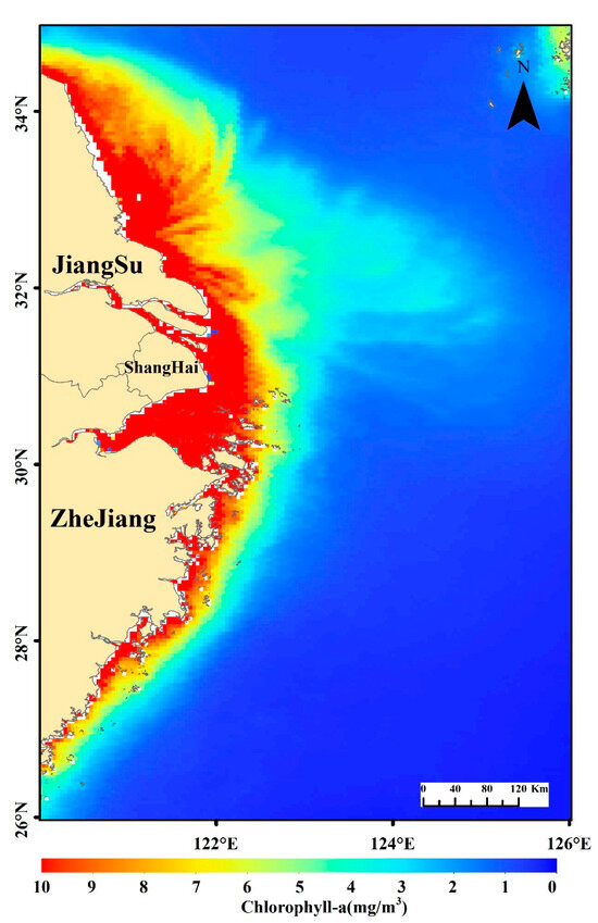
Figure 1.
Spatial distribution of the annual average chlorophyll-a (Chl-a) concentration derived from satellite observations in the study area, covering the period from 1998–2023.
2.2. Methods
2.2.1. ConvLSTM Neural Network
ConvLSTM is a deep learning model that integrates the strengths of CNNs and LSTM networks [43]. This model is designed to process sequential data while effectively capturing complex spatiotemporal patterns. The core concept of ConvLSTM is the integration of a convolutional structure with LSTM, allowing the network to consider spatial correlations during input-to-state and state-to-state transitions. This structure is particularly effective for processing spatiotemporal data with spatial correlations, such as video and meteorological radar images [44,45,46].
The ConvLSTM network consists of three parts, the forget gate, the input gate and the output gate, as follows:
In this context, , , , and represent the forget gate, input gate, memory cell, and output gate, respectively. and represent the input and hidden states at time t, respectively, and and represent the memory cell and hidden state at the previous time step (t−1), respectively. and represent the weight matrix and bias vector, respectively. and refer to the sigmoid and hyperbolic tangent activation functions, respectively. ‘*’ denotes convolution, and ‘⨀’ denotes the Hadamard product.
2.2.2. Structure of the Chlorophyll-a Concentration Prediction Model
In this study, an ocean Chl-a concentration prediction model (ChlaPM) was developed using the ConvLSTM neural network. This model comprises three modules: the recent spatiotemporal feature extraction (RSTFE), periodic feature extraction (PFE), and denoise fusion (DNF) modules (Figure 2).
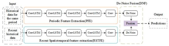
Figure 2.
Architecture of the chlorophyll-a concentration prediction model, with the RSTFE, PFE, and DNF modules.
Recent Chl-a concentrations significantly influence future changes [47]. To address this, the RSTFE module is introduced to leverage historical data and capture complex spatiotemporal correlations in future Chl-a concentrations. The module comprises four stacked ConvLSTM layers and one convolutional layer to capture both the temporal sequence characteristics and spatial distribution features of Chl-a concentrations.
Considering the significant periodic changes in marine Chl-a concentrations, the PFE module is incorporated to extract and predict the periodic characteristics corresponding to the target month on the basis of historical data. The PFE module shares a similar structure with the RSTFE module but uses historical Chl-a concentration data from the same period as input, effectively capturing seasonal patterns.
To mitigate prediction errors caused by noisy areas (e.g., land and islands) that affect spatial feature extraction during convolution operations, the DNF module is introduced. This module eliminates noise from the outputs of the RSTFE and PFE modules and integrates them to produce the final prediction. Linear transformations are applied to the RSTFE and PFE outputs (denoted as and , respectively) for denoising, resulting in features and , which are fused to generate the final prediction . The formula is as follows:
Here, and are learnable weight matrices, with each element corresponding to weights for spatial positions and feature channels. These matrices are optimized through network training, enabling feature intensity adjustments on the basis of the statistical distribution of historical data, thereby mitigating noise interference.
To ensure stable convergence and optimal feature representation, the model parameters were configured through systematic experimentation. The ConvLSTM layers in both the RSTFE and PFE modules have a symmetric kernel configuration (6, 12, 12, 6) with 3 × 3 convolutional kernels, a structure empirically proven to balance computational efficiency and multiscale spatiotemporal feature extraction. Zero padding is uniformly applied to maintain spatial dimensions across layers, which is critical for preserving coastal boundary details in Chl-a prediction. The final convolutional layers in RSTFE and PFE utilize single 3 × 3 kernels to compress features while avoiding oversmoothing.
2.2.3. Methodology and Process
This study comprises three main stages: data preprocessing, model training, and model evaluation. The Chl-a dataset is prepared through preprocessing steps, such as cropping the research area, filling missing values, and applying masking techniques. The complete Chl-a dataset is split into independent training, validation, and test sets. Three models—RSTFE, RSTFE+PFE, and ChlaPM—are employed for training and to predict Chl-a concentrations. The corresponding flowchart is illustrated in Figure 3.
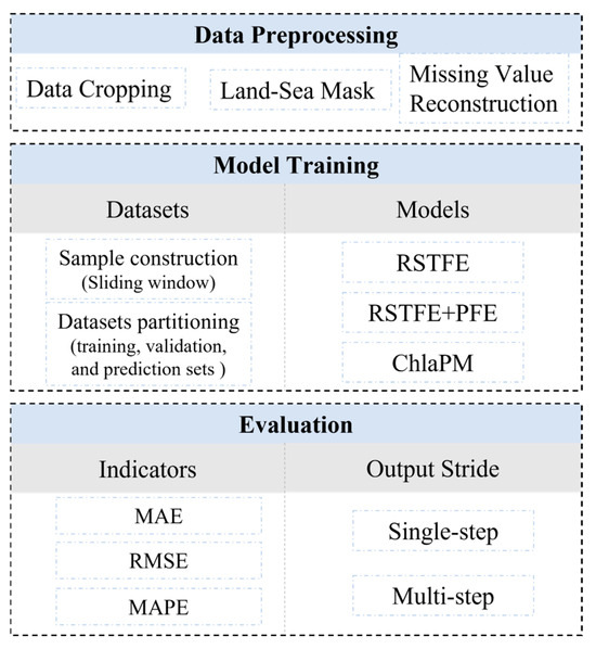
Figure 3.
Flowchart of the Chl-a concentration prediction process.
2.2.4. Data Preprocessing
Data preprocessing comprises three key steps: cropping and masking, filling in missing values, and constructing datasets.
Step 1: Cropping and masking. The original Chl-a concentration data are cropped on the basis of the boundaries of the study area, which are defined using geographical coordinates or administrative region boundaries. Masking is then applied to exclude terrestrial rivers and lakes, leaving only oceanic Chl-a concentration data.
Step 2: Filling in missing values. Factors such as weather conditions and high solar radiation contamination result in missing values in satellite remote sensing Chl-a datasets. To address this issue, the data interpolation empirical orthogonal function (DINEOF) method is employed in this study. DINEOF is widely used in marine remote sensing because it effectively handles gaps in large-scale datasets and preserves the spatial and temporal structures of the data. This method works by decomposing the data matrix into empirical orthogonal functions and reconstructing missing values on the basis of the spatial and temporal relationships among observed data points [48]. In this study, the DINEOF reconstruction process is optimized through parameter selection to ensure accuracy and computational efficiency. The number of EOF modes ranges from a minimum of 1 (neini) to a maximum of 5 (nev), and the Krylov subspace size (ncv) is set to 10 to provide adequate computational capacity for the Lanczos solver. The convergence tolerance (tol) is defined as 1.0 × 10−⁸, ensuring precise reconstruction, with a maximum iteration count (nitemax) of 300 and an iteration stopping threshold (toliter) of 1.0 × 10⁻³ to stabilize the EOF estimation process. These settings increase the robustness of the reconstruction process, ensuring that complete and reliable sea surface Chl-a concentration data are obtained for subsequent analysis.
Step 3: Constructing datasets. The dataset is temporally partitioned into training, validation, and prediction sets. The monthly composite Chl-a imagery products span from January 1998 to December 2023, comprising 312 monthly averaged raster grids. Among these images, 276 composite images (January 1998–December 2020) are allocated for model training and validation, with the most recent 36 temporal slices (January 2021–December 2023) reserved for predictive evaluation.
2.2.5. Evaluation Indicators
In this study, the model’s performance was evaluated using three metrics: the mean absolute error (MAE), root mean square error (RMSE), and mean absolute percentage error (MAPE). The corresponding formulas are as follows:
Here, denotes the model-predicted value, and represents the observed satellite value. Low MAE, RMSE, and MAPE values indicate high model prediction accuracy.
3. Results
3.1. Spatiotemporal Evaluation of the Chl-a Prediction Model
To analyze the effects of different modules on Chl-a prediction, three models are developed in this study: the RSTFE model, which uses only recent historical data; the RSTFE+PFE model, which uses integrated periodic data; and the ChlaPM model, which incorporates a noise removal module. The objective of this experiment is to compare how these models perform in predicting Chl-a concentrations, with a particular focus on their ability to capture temporal patterns, reduce prediction errors, and analyze spatial discrepancies. This includes evaluating how well each model addresses both the temporal trends in Chl-a concentrations and the spatial errors in the predictions. Recent historical data span the previous six months, whereas periodic data comprise same-month historical data from the past three years, which are used to predict the Chl-a concentration in the subsequent month.
Figure 4 presents the temporal trends in the spatially averaged Chl-a prediction results for RSTFE, RSTFE+PFE, and ChlaPM. Compared with the RSTFE+PFE model, the ChlaPM predictions closely align with the observed Chl-a variations. This improvement is due to the integration of the noise removal module in ChlaPM, which enhances it to capture future Chl-a trends by extracting both spatiotemporal patterns from the data. In this study, the observed average Chl-a concentration peaked in January 2022 and reached its annual minimum in June 2023. In contrast, the RSTFE model predicted peaks in February 2022 and troughs in July 2023, exhibiting a “lag” phenomenon. This discrepancy likely arose because the RSTFE module relies solely on recent trends and lacks the cyclical data necessary to identify turning points in Chl-a trends. However, the RSTFE+PFE and ChlaPM models, which incorporate periodic information, predict changes that align with the actual temporal trend of the Chl-a concentration. Although ChlaPM performs well overall, noticeable discrepancies remain between the model predictions and actual values in certain months. These discrepancies can be attributed to several factors, such as the complexity of spatiotemporal variations in Chl-a concentrations, which are influenced by dynamic environmental conditions such as seasonal changes, nutrient availability, and various oceanographic processes.
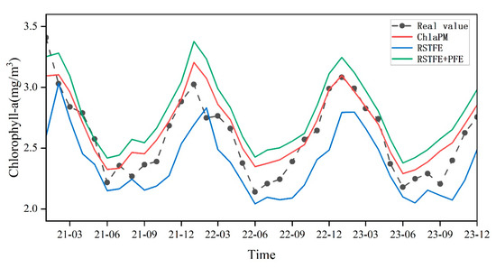
Figure 4.
Monthly average Chl-a change trends for the test set and comparison of the prediction results from the three models.
Figure 5 shows the average Chl-a predictions and corresponding average RMSEs of RSTFE, RSTFE+PFE, and ChlaPM across different calendar months. As depicted in panel (a), ChlaPM consistently produces predicted Chl-a concentrations that closely match the observed values, particularly in summer and autumn. Moreover, the average RMSEs of the RSTFE+PFE model and ChlaPM, which incorporate cyclical data, are significantly lower than those of RSTFE across all months, as shown in panel (b). These findings suggest that cyclical characteristics play a critical role in marine Chl-a prediction, with models that account for these factors demonstrating improved performance.
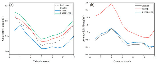
Figure 5.
Performance analysis of the Chl-a prediction models across different calendar months. (a) Comparison of Chl-a prediction values for ChlaPM, RSTFE, and RSTFE + PFE across different calendar months; (b) comparison of RMSE values for the Chl-a predictions of ChlaPM, RSTFE, and RSTFE + PFE across different calendar months.
The spatial distribution of the Chl-a concentration in the study area displays notable seasonal variations. Figure 6 shows the seasonal distributions of satellite observations and model predictions for the three models. In high-value areas near the shore, particularly along Jiangsu Province’s coastal waters, the RSTFE model predictions are lower than the observed values, whereas the RSTFE+PFE model predictions exceed the observations. The RSTFE+PFE model and ChlaPM more accurately simulate seasonal changes, with ChlaPM predictions near the shore and at great distances from the shore display notably higher accuracy. The MAEs between the RSTFE model predictions and observations are relatively high (Figure 7). Inaccuracies are primarily concentrated in areas with relatively high Chl-a concentrations, particularly along the coastal waters of Jiangsu Province and Hangzhou Bay. This phenomenon may be attributed to the limited capacity of the standalone RSTFE module to distinguish short-term fluctuations from persistent periodic signals in these dynamic coastal ecosystems. The integration of the PFE module into the model effectively addresses this limitation. Compared with the RSTFE model, the RSTFE+PFE model results in lower prediction errors and no significant seasonal differences in spatial distribution. This improvement underscores the critical role of explicit periodic feature extraction in mitigating prediction biases caused by cyclic environmental drivers. ChlaPM further elevates prediction fidelity through its denoising fusion mechanism, and the MAEs between the ChlaPM model predictions and observations are small, with significantly improved prediction accuracy near the shore. However, the ChlaPM model still performs poorly in Hangzhou Bay, likely because of the highly turbid waters and rapid spatiotemporal changes in the bay and its adjacent areas, where Chl-a concentration fluctuations are influenced by multiple factors, making it difficult to identify the corresponding spatiotemporal evolution patterns.
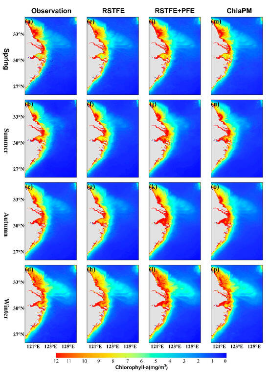
Figure 6.
Spatial distributions of satellite observations and model predictions across the four seasons. (a–d) Distributions of chlorophyll-a observed by satellites during spring, summer, autumn, and winter. Distributions of predictions from (e–h) the RSTFE model, (i–l) the RSTFE+PFE model, and (m–p) the ChlaPM model.
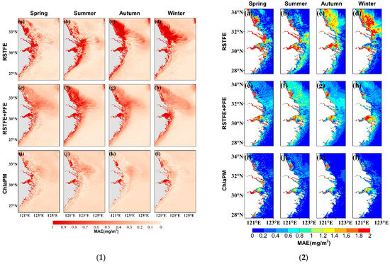
Figure 7.
Spatial distributions of the MAEs between the Chl-a values predicted by the three models and the satellite-observed Chl-a values across the four seasons. For (1) Overall study area and (2) Coastal area: (a–d) MAE distributions between the RSTFE model predictions and satellite observations for spring, summer, autumn, and winter; (e–h) MAE distributions between the RSTFE+PFE model predictions and satellite observations; and (i–l) MAE distributions between the ChlaPM model predictions and satellite observations.
To further evaluate the spatial prediction accuracy of the three models, we analyzed the root mean square error (RMSE) distributions across the study area. As shown in Figure 8a,the RMSE of the RSTFE model predictions is greatest in areas with high and medium Chl-a concentrations. Figure 8b illustrates that the RMSE distribution of the RSTFE+PFE model closely follows that of the RSTFE model but with overall lower absolute error values. Compared with the RSTFE+PFE model, the RMSE of the ChlaPM model predictions is significantly lower, with only a few coastal areas exhibiting higher RMSE values (Figure 8c). This improvement highlights the effectiveness of the noise removal fusion (DNF) module for reducing prediction errors by enhancing the model’s ability to capture spatiotemporal patterns.
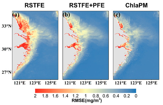
Figure 8.
Spatial distributions of the Chl-a RMSEs predicted by the three models. (a) RMSE distribution between RSTFE model predictions and satellite observations, (b) RMSE distribution between RSTFE+PFE model predictions and satellite observations, and (c) RMSE distribution between ChlaPM model predictions and satellite observations.
In summary, the ChlaPM model demonstrates significantly improved consistency with actual values in both spatial and temporal analyses after incorporating periodic features and the DNF module. The integration of these components enables the ChlaPM model to effectively capture complex spatiotemporal patterns, reducing prediction errors and aligning predicted trends closely with observed Chl-a concentrations. As a next step, further analysis will be conducted to evaluate the performance of the ChlaPM model across different prediction horizons and explore its robustness and effectiveness in multistep forecasting scenarios.
3.2. Analysis of the Prediction Performance at Different Step Lengths
To comprehensively evaluate the effectiveness of the ChlaPM model in predicting Chl-a concentrations, we analyzed its performance across different prediction horizons: 1 month, 3 months, and 6 months. This analysis not only highlighted the model’s capability for both short- and long-term predictions but also contributed to optimizing its structure and improving its predictive accuracy. To assess the relative performance, we conducted comparative experiments using the LSTM, CNN-LSTM, RSTFE, and RSTFE+PFE models. The LSTM and CNN-LSTM models were consistent with those proposed by Cen et al. [49] and Liu et al. [28], respectively, for Chl-a prediction. These comparisons provided a comprehensive benchmark for evaluating the predictive advantages of ChlaPM.
Table 1 presents the RMSE, MAE, and MAPE results for the RSTFE, RSTFE+PFE, ChlaPM, LSTM, and CNN-LSTM models in predicting the Chl-a concentration. As shown in Table 1, all the models perform well in 1-month-ahead prediction. However, their performance declines as the prediction horizon extends. The RSTFE model consistently performs worse than the RSTFE+PFE and ChlaPM models at all prediction horizons. The LSTM model performs well in short-term predictions, but its performance gradually deteriorates as the prediction horizon extends. Additionally, while the CNN-LSTM model is less accurate than the LSTM model is, it exhibits greater stability in long-term prediction. The ChlaPM model exhibits stable performance over longer prediction horizons, but its accuracy decreases as the forecasting period extends. The decline is less pronounced than that for the other models, indicating its advantage in terms of long-term prediction stability.

Table 1.
Chl-a prediction performance. “1-step”, “3-step”, and “6-step” refer to predictions for the next 1 month, 3 months, and 6 months, respectively.
Figure 9 shows the spatial distribution of the MAEs for three-step predictions using ChlaPM, with average MAEs of 0.264 mg·m−3, 0.275 mg·m−3, and 0.276 mg·m−3. In offshore deep-water areas far from land, where the Chl-a values are smaller and less variable than those closer to land, the prediction errors do not change significantly as the prediction step length increases. However, in coastal regions close to land, such as the offshore areas of Jiangsu Province and Hangzhou Bay, the prediction errors are large and increase with increasing prediction step length. In brief, the ChlaPM model outperforms RSTFE and RSTFE+PFE, offering greater stability and accuracy, especially for long-term predictions, and shows strong potential for use in diverse marine applications.
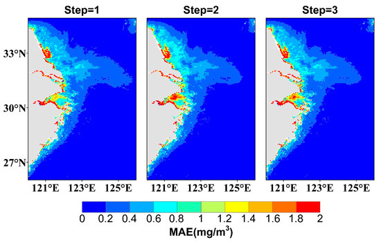
Figure 9.
Spatial distributions of the MAEs for the Chl-a predictions obtained with ChlaPM for the next 3 steps (months). Steps 1, 2, and 3 correspond to predictions for the first, second, and third months, respectively.
4. Discussion
Large-scale and high-precision prediction of marine Chl-a concentrations is crucial for preventing algal blooms and mitigating marine environmental pollution. The aim of this study was to address the challenges posed by short-term spatiotemporal variability and periodic changes in Chl-a concentrations while considering the effects of terrestrial and island regions on prediction accuracy. To achieve this goal, three deep learning models, RSTFE, RSTFE+PFE, and ChlaPM, were trained and applied to improve the accuracy of Chl-a concentration predictions.
4.1. Advantages and Contributions of the Models
4.1.1. Limitations and Drawbacks of Existing Models
The ConvLSTM model, known for its ability to capture temporal dynamics and spatial features simultaneously, is extensively used in applications such as sea surface temperature prediction and precipitation forecasting. This model performs particularly well in handling complex spatiotemporal data in the Earth sciences. Despite their ability to capture spatiotemporal trends in Chl-a concentrations, ConvLSTM-based RSTFE models have notable limitations in predicting marine Chl-a concentrations, particularly underestimating high nearshore concentrations and failing to capture seasonal inflection points.
In single-step spatiotemporal prediction, the RSTFE model generally yields worse results than other models. This is primarily due to the assignment of zero values for Chl-a concentrations in nonmarine areas, such as land and islands, in the model input set. Since no actual Chl-a concentration data exist in these areas, this approach interferes with spatial feature extraction in nearshore regions during convolution, leading to an underestimation of Chl-a concentrations in these areas.
Additionally, the RSTFE model has significant limitations in simulating seasonal variations in Chl-a concentrations, particularly in capturing critical inflection points. Following increases in Chl-a concentrations, the model tends to overestimate the concentration in the subsequent month; conversely, it underestimates these values when concentrations decrease. This issue arises from the RSTFE model’s reliance on recent spatiotemporal trends for prediction, thus failing to consider the periodic and seasonal characteristics of Chl-a concentration changes and limiting its predictive accuracy.
4.1.2. Role of Periodic Characteristics and Spatial Denoising in Chl-a Prediction
The PFE and DNF modules based on the RSTFE model are introduced in this study to accurately predict dynamic changes in the Chl-a concentration. These improvements enhance the model’s ability to simulate seasonal variations and correct prediction biases caused by mask areas and spatial heterogeneity.
The periodic feature extraction module captures the long-term variation patterns of Chl-a concentrations, such as annual cycles and seasonal characteristics, addressing the limitations of basic models (e.g., the RSTFE model) that rely only on recent spatiotemporal trends. The experimental results show that the RSTFE+PFE model more accurately predicts the inflection points of Chl-a concentration changes, reducing both overestimation and underestimation. This module demonstrates excellent adaptability, particularly at time nodes of significant change, such as seasonal transitions or peak Chl-a concentration periods, thereby enhancing prediction accuracy. These improvements address a critical gap in existing models, which often fail to capture rapid fluctuations and turning points in Chl-a dynamics. By effectively integrating periodic information, this module not only enhances the precision of spatiotemporal predictions but also provides a framework for understanding complex environmental patterns.
The ChlaPM model employs linear transformation techniques to eliminate prediction biases caused by mask areas and spatial heterogeneity in the ocean. Figure 10 shows the linear transformation denoising coefficient matrices and produced by the RSTFE and PFE modules in the ChlaPM model. First, the coefficient matrix captures spatial distribution characteristics in land–sea boundary areas. Low values in terrestrial and island regions indicate that the model effectively suppresses or ignores output interference, avoiding misleading predictions due to zero-mask effects. In marine areas near land edges, such as coastal transitional zones, the denoising coefficient matrix includes high values, suggesting that the model amplifies outputs in these critical areas, correcting underestimation biases associated with the treatment of values in terrestrial regions. In areas with high Chl-a concentrations, such as Hangzhou Bay and Jiangsu coastal waters, the denoising coefficient matrix includes significantly higher values, reflecting the model’s fine adjustments in regions with substantial seasonal fluctuations and capturing complex concentration variations. In summary, the ChlaPM model effectively mitigates the impact of mask areas and ocean spatial heterogeneity on Chl-a concentration prediction by using a learnable linear transformation coefficient matrix, resulting in significant improvements in simulating seasonal variations. This finding provides a new perspective for predicting marine Chl-a concentrations and offers valuable insights for applying deep learning models in marine remote sensing applications.
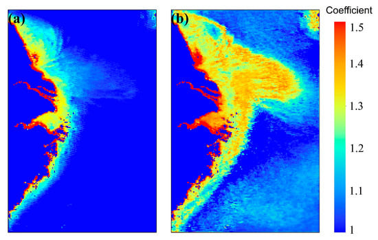
Figure 10.
Linear transformation denoising coefficient matrices of the ChlaPM model: (a) represents the matrix from the RSTFE module output, and (b) represents the matrix from the PFE module output.
4.2. Generalizability and Limitations of the Model
To evaluate the scalability and broad applicability of the ChlaPM model, we conducted a cross-regional validation in a selected region within the Yellow Bohai Sea (YBS), a semi-enclosed sea in northern China. The study area spans 32–45°N and 114–127°E, covering diverse marine environments [29,50]. We compared the predictive performance of the RSTFE, RSTFE+PFE, and ChlaPM models in 6-month Chl-a concentration forecasting. The results, summarized in Table 2, show that ChlaPM achieved the lowest RMSE (0.604), MAE (0.185), and MAPE (0.412%). The significantly lower MAPE than that of the other models indicates that ChlaPM provides more stable and consistent predictions across different concentration levels, a crucial advantage for water quality monitoring and early warning provision for ecological disasters. The cross-regional validation results in this selected YBS region further confirm the generalizability of ChlaPM beyond the original study area. Across key evaluation metrics (RMSE, MAE, and MAPE), ChlaPM consistently outperforms the baseline models (RSTFE and RSTFE+PFE), demonstrating its adaptability to marine environments with varying spatiotemporal characteristics. This result underscores the strong feature extraction ability of ChlaPM, particularly its effectiveness in filtering out noise from nonmarine regions and capturing the periodic variations in Chl-a concentrations.
Table 2.
Cross-regional validation in the Yellow Bohai Sea: Performance comparison of chlorophyll concentration prediction models for a 6-month forecasting horizon.
Despite the excellent overall performance of the ChlaPM model, it has limitations in obtaining accurate predictions in specific regions, such as Hangzhou Bay. These limitations stem from high Chl-a concentrations, steep spatial gradients, and complex anthropogenic and environmental interactions in these regions. These factors complicate the prediction of Chl-a concentrations. However, these limitations do not undermine the overall findings of the study, as the predictive results in these regions remain valuable, offering important scientific references for monitoring and managing long-term marine trends. The ChlaPM model can be applied in large-scale environmental monitoring systems to predict oceanic trends and aid in the early detection of potential algal blooms. Additionally, it can be applied in coastal zone management, provide insights for sustainable fisheries and help mitigate marine pollution by forecasting Chl-a concentration fluctuations over extended periods.
Future studies could be conducted to optimize the ChlaPM model to better consider complex environmental conditions in specific regions. Specifically, incorporating additional environmental variables (e.g., water temperature, flow rate, and nutrient concentration) and anthropogenic activity data (e.g., aquaculture and industrial emissions) into the model could enhance its adaptability to local conditions. As a preliminary step, historical water temperature and flow rate data could be integrated into ChlaPM to assess their influence on predictive performance. Additionally, feature selection techniques such as correlation analysis and attention mechanisms could be employed to determine the most impactful variables. These enhancements could refine the model’s ability to distinguish between seasonal variability and short-term disturbances in highly dynamic environments. Additionally, cross-validation across different marine environments could improve the model’s generalizability and enhance its predictive performance in diverse scenarios.
These improvements will increase prediction accuracy and applicability, providing stronger support for large-scale Chl-a concentration prediction, marine ecological monitoring, and algal bloom prevention.
5. Conclusions
This study aimed to address the challenge of accurately predicting marine Chl-a concentrations by introducing a ConvLSTM-based model, ChlaPM, which captures short-term spatiotemporal characteristics and periodic changes in Chl-a concentrations. Previous models struggled with accurately predicting seasonal inflection points and high nearshore concentrations because of the complex nature of marine environments. In contrast, the ChlaPM model not only effectively handles these challenges but also eliminates noise from nontarget areas such as land, improving the overall prediction accuracy.
Training and validating the ChlaPM model with the monthly average OC-CCI Chl-a dataset from the East China Sea confirmed that the model outperformed existing methods in single-step prediction and displayed greater stability in multistep prediction. Specifically, for 1-, 3-, and 6-month Chl-a concentration prediction, compared with the existing methods, the ChlaPM model yielded RMSE reductions of 53.84%, 53.58%, and 49.70%, respectively. The ChlaPM model can also effectively handle heterogeneous spatial distributions and wide concentration ranges, achieving large-scale, synchronous predictions with high efficiency and stability.
While the ChlaPM model displayed excellent overall performance, its prediction accuracy can still be improved in specific small areas with high Chl-a concentrations and steep gradients. Future work will focus on developing specialized models for regions with complex Chl-a concentration changes to improve predictive accuracy. We will also explore integrating additional environmental and meteorological factors into the model and optimizing the model structure and algorithms to capture more comprehensive spatiotemporal features and improve prediction accuracy. These efforts could provide more reliable scientific support for marine environmental monitoring and ecological protection.
Author Contributions
Conceptualization, D.W. and Q.T.; methodology, Q.R.; software, Q.R.; validation, Q.R.; formal analysis, Q.R.; resources, D.P., D.W. and F.G.; writing—original draft preparation, Q.R.; writing—review and editing, D.W. and X.H.; supervision, project administration and funding acquisition, D.W. and X.H. All authors have read and agreed to the published version of the manuscript.
Funding
This research was funded by the National Natural Science Foundation of China under contract Nos. 42476174 and 41476157 and the National Key R&D Program of China under Grant Nos. 2018YFB0505005 and 2017YFC1405300.
Data Availability Statement
Publicly available datasets were analyzed in this study. Chlorophyll-a data from satellite observations can be found at https://climate.esa.int/en/projects/ocean-colour/; accessed on 10 June 2024.
Acknowledgments
The authors would like to thank the European Space Agency for the excellent chlorophyll-a concentration data. We also thank the satellite ground station personnel and the satellite data processing and sharing center of SOED/SIO for assisting with the data processing. Our deepest gratitude goes to the editors and reviewers for their careful work and thoughtful suggestions.
Conflicts of Interest
The authors declare no conflicts of interest.
References
- Lee, Y.J.; Matrai, P.A.; Friedrichs, M.A.M.; Saba, V.S.; Antoine, D.; Ardyna, M.; Asanuma, I.; Babin, M.; Bélanger, S.; Benoît-Gagné, M.; et al. An Assessment of Phytoplankton Primary Productivity in the Arctic Ocean from Satellite Ocean Color/in Situ Chlorophyll- a Based Models. JGR Oceans 2015, 120, 6508–6541. [Google Scholar] [CrossRef]
- Wu, J.; Goes, J.I.; Do Rosario Gomes, H.; Lee, Z.; Noh, J.-H.; Wei, J.; Shang, Z.; Salisbury, J.; Mannino, A.; Kim, W.; et al. Estimates of Diurnal and Daily Net Primary Productivity Using the Geostationary Ocean Color Imager (GOCI) Data. Remote Sens. Environ. 2022, 280, 113183. [Google Scholar] [CrossRef]
- Sharada, M.K.; Yajnik, K.S. Seasonal Variation of Chlorophyll and Primary Productivity in Central Arabian Sea: A Macrocalibrated Upper Ocean Ecosystem Model. Proc. Indian Acad. Sci. (Earth Planet Sci.) 1997, 106, 33–42. [Google Scholar] [CrossRef]
- Iriarte, J.L.; González, H.E.; Liu, K.K.; Rivas, C.; Valenzuela, C. Spatial and Temporal Variability of Chlorophyll and Primary Productivity in Surface Waters of Southern Chile (41.5–43° S). Estuar. Coast. Shelf Sci. 2007, 74, 471–480. [Google Scholar] [CrossRef]
- Hao, Y.; Tang, D.; Yu, L.; Xing, Q. Nutrient and Chlorophyll a Anomaly in Red-Tide Periods of 2003–2008 in Sishili Bay, China. Chin. J. Ocean. Limnol. 2011, 29, 664–673. [Google Scholar] [CrossRef]
- Yu, P.; Gao, R.; Zhang, D.; Liu, Z.-P. Predicting Coastal Algal Blooms with Environmental Factors by Machine Learning Methods. Ecol. Indic. 2021, 123, 107334. [Google Scholar] [CrossRef]
- Liu, R.; Xiao, Y.; Ma, Y.; Cui, T.; An, J. Red Tide Detection Based on High Spatial Resolution Broad Band Optical Satellite Data. ISPRS J. Photogramm. Remote Sens. 2022, 184, 131–147. [Google Scholar] [CrossRef]
- Dutkiewicz, S.; Hickman, A.E.; Jahn, O.; Henson, S.; Beaulieu, C.; Monier, E. Ocean Colour Signature of Climate Change. Nat. Commun. 2019, 10, 578. [Google Scholar] [CrossRef] [PubMed]
- Gao, S.; Ren, S.; Xie, B.; Zhang, S.; Lu, J.; Fu, G. Interaction between Sea Surface Chlorophyll a and Seawater Indicators in the Sea Ranching Area: A Case Study in Haizhou Bay. Reg. Stud. Mar. Sci. 2022, 56, 102687. [Google Scholar] [CrossRef]
- Park, T.G.; Lim, W.A.; Park, Y.T.; Lee, C.K.; Jeong, H.J. Economic Impact, Management and Mitigation of Red Tides in Korea. Harmful Algae 2013, 30, S131–S143. [Google Scholar] [CrossRef]
- Hamilton, D.P.; Schladow, S.G. Prediction of Water Quality in Lakes and Reservoirs. Part I—Model Description. Ecol. Model. 1997, 96, 91–110. [Google Scholar] [CrossRef]
- Los, F.J.; Villars, M.T.; Van Der Tol, M.W.M. A 3-Dimensional Primary Production Model (BLOOM/GEM) and Its Applications to the (Southern) North Sea (Coupled Physical–Chemical–Ecological Model). J. Mar. Syst. 2008, 74, 259–294. [Google Scholar] [CrossRef]
- Allen, M.; Frame, D.; Kettleborough, J.; Stainforth, D. Model Error in Weather and Climate Forecasting. In Predictability of Weather and Climate; Palmer, T., Hagedorn, R., Eds.; Cambridge University Press: Cambridge, UK, 2006; pp. 391–427. ISBN 978-0-521-84882-4. [Google Scholar]
- Li, H.; Li, X.; Song, D.; Nie, J.; Liang, S. Prediction on Daily Spatial Distribution of Chlorophyll-a in Coastal Seas Using a Synthetic Method of Remote Sensing, Machine Learning and Numerical Modeling. Sci. Total Environ. 2024, 910, 168642. [Google Scholar] [CrossRef]
- Uddameri, V.; Silva, A.; Singaraju, S.; Mohammadi, G.; Hernandez, E. Tree-Based Modeling Methods to Predict Nitrate Exceedances in the Ogallala Aquifer in Texas. Water 2020, 12, 1023. [Google Scholar] [CrossRef]
- Lee, S.; Lee, D. Improved Prediction of Harmful Algal Blooms in Four Major South Korea’s Rivers Using Deep Learning Models. Int. J. Environ. Res. Public Health 2018, 15, 1322. [Google Scholar] [CrossRef]
- Bourel, M.; Crisci, C.; Martínez, A. Consensus Methods Based on Machine Learning Techniques for Marine Phytoplankton Presence–Absence Prediction. Ecol. Inform. 2017, 42, 46–54. [Google Scholar] [CrossRef]
- Mamun, M.; Kim, J.-J.; Alam, M.A.; An, K.-G. Prediction of Algal Chlorophyll-a and Water Clarity in Monsoon-Region Reservoir Using Machine Learning Approaches. Water 2019, 12, 30. [Google Scholar] [CrossRef]
- Kruk, M. Prediction of Environmental Factors Responsible for Chlorophyll A-Induced Hypereutrophy Using Explainable Machine Learning. Ecol. Inform. 2023, 75, 102005. [Google Scholar] [CrossRef]
- Tian, W.; Liao, Z.; Zhang, J. An Optimization of Artificial Neural Network Model for Predicting Chlorophyll Dynamics. Ecol. Model. 2017, 364, 42–52. [Google Scholar] [CrossRef]
- Yu, Z.; Yang, K.; Luo, Y.; Shang, C. Spatial-Temporal Process Simulation and Prediction of Chlorophyll-a Concentration in Dianchi Lake Based on Wavelet Analysis and Long-Short Term Memory Network. J. Hydrol. 2020, 582, 124488. [Google Scholar] [CrossRef]
- Waqas, M.; Humphries, U.W. A Critical Review of RNN and LSTM Variants in Hydrological Time Series Predictions. MethodsX 2024, 13, 102946. [Google Scholar] [CrossRef]
- Karevan, Z.; Suykens, J.A.K. Transductive LSTM for Time-Series Prediction: An Application to Weather Forecasting. Neural Netw. 2020, 125, 1–9. [Google Scholar] [CrossRef] [PubMed]
- Gitelson, A.A.; Schalles, J.F.; Hladik, C.M. Remote Chlorophyll-a Retrieval in Turbid, Productive Estuaries: Chesapeake Bay Case Study. Remote Sens. Environ. 2007, 109, 464–472. [Google Scholar] [CrossRef]
- Shen, F.; Tang, R.; Sun, X.; Liu, D. Simple Methods for Satellite Identification of Algal Blooms and Species Using 10-Year Time Series Data from the East China Sea. Remote Sens. Environ. 2019, 235, 111484. [Google Scholar] [CrossRef]
- Indolia, S.; Goswami, A.K.; Mishra, S.P.; Asopa, P. Conceptual Understanding of Convolutional Neural Network- A Deep Learning Approach. Procedia Comput. Sci. 2018, 132, 679–688. [Google Scholar] [CrossRef]
- Liu, R.; Cui, B.; Dong, W.; Fang, X.; Xiao, Y.; Zhao, X.; Cui, T.; Ma, Y.; Wang, Q. A Refined Deep-Learning-Based Algorithm for Harmful-Algal-Bloom Remote-Sensing Recognition Using Noctiluca Scintillans Algal Bloom as an Example. J. Hazard. Mater. 2024, 467, 133721. [Google Scholar] [CrossRef]
- Na, L.; Shaoyang, C.; Zhenyan, C.; Xing, W.; Yun, X.; Li, X.; Yanwei, G.; Tingting, W.; Xuefeng, Z.; Siqi, L. Long-Term Prediction of Sea Surface Chlorophyll-a Concentration Based on the Combination of Spatio-Temporal Features. Water Res. 2022, 211, 118040. [Google Scholar] [CrossRef]
- Yao, L.; Wang, X.; Zhang, J.; Yu, X.; Zhang, S.; Li, Q. Prediction of Sea Surface Chlorophyll-a Concentrations Based on Deep Learning and Time-Series Remote Sensing Data. Remote Sens. 2023, 15, 4486. [Google Scholar] [CrossRef]
- Ye, M.; Li, B.; Nie, J.; Wen, Q.; Wei, Z.; Yang, L.-L. Graph Convolutional Network-Assisted SST and Chl-a Prediction With Multicharacteristics Modeling of Spatio-Temporal Evolution. IEEE Trans. Geosci. Remote Sens. 2023, 61, 4209214. [Google Scholar] [CrossRef]
- Chen, J.; Ma, T.; Xiao, C. FastGCN: Fast Learning with Graph Convolutional Networks via Importance Sampling. arXiv 2018, arXiv:1801.10247. [Google Scholar]
- Liu, X.; Xiao, W.; Landry, M.R.; Chiang, K.-P.; Wang, L.; Huang, B. Responses of Phytoplankton Communities to Environmental Variability in the East China Sea. Ecosystems 2016, 19, 832–849. [Google Scholar] [CrossRef]
- Kim, D.; Shim, J.; Yoo, S. Seasonal Variations in Nutrients and Chlorophyll-a Concentrations in the Northern East China Sea. Ocean Sci. J. 2006, 41, 125–137. [Google Scholar] [CrossRef]
- Jiang, Q.; He, J.; Wu, J.; Hu, X.; Ye, G.; Christakos, G. Assessing the Severe Eutrophication Status and Spatial Trend in the Coastal Waters of Zhejiang Province (China). Limnol. Oceanogr. 2019, 64, 3–17. [Google Scholar] [CrossRef]
- Guo, S.; Feng, Y.; Wang, L.; Dai, M.; Liu, Z.; Bai, Y.; Sun, J. Seasonal Variation in the Phytoplankton Community of a Continental-Shelf Sea: The East China Sea. Mar. Ecol. Prog. Ser. 2014, 516, 103–126. [Google Scholar] [CrossRef]
- Gong, G.-C.; Wen, Y.-H.; Wang, B.-W.; Liu, G.-J. Seasonal Variation of Chlorophyll a Concentration, Primary Production and Environmental Conditions in the Subtropical East China Sea. Deep Sea Res. Part II Top. Stud. Oceanogr. 2003, 50, 1219–1236. [Google Scholar] [CrossRef]
- Yuan, Z.; Xiao, X.; Wang, F.; Xing, L.; Wang, Z.; Zhang, H.; Xiang, R.; Zhou, L.; Zhao, M. Spatiotemporal Temperature Variations in the East China Sea Shelf during the Holocene in Response to Surface Circulation Evolution. Quat. Int. 2018, 482, 46–55. [Google Scholar] [CrossRef]
- Wang, X.H.; Cho, Y.-K.; Guo, X.; Wu, C.-R.; Zhou, J. The Status of Coastal Oceanography in Heavily Impacted Yellow and East China Sea: Past Trends, Progress, and Possible Futures. Estuar. Coast. Shelf Sci. 2015, 163, 235–243. [Google Scholar] [CrossRef]
- Zhao, Y.; Chen, P.; Zheng, G.; Wang, D.; Yang, J.; Li, X.; Luo, D. Fine Spatio-Temporal Prediction of Fishing Time Using Big Data. Front. Mar. Sci. 2024, 11, 1421188. [Google Scholar] [CrossRef]
- Zhou, Y.; Yan, W.; Wei, W. Effect of Sea Surface Temperature and Precipitation on Annual Frequency of Harmful Algal Blooms in the East China Sea over the Past Decades. Environ. Pollut. 2021, 270, 116224. [Google Scholar] [CrossRef]
- Lou, X.; Hu, C. Diurnal Changes of a Harmful Algal Bloom in the East China Sea: Observations from GOCI. Remote Sens. Environ. 2014, 140, 562–572. [Google Scholar] [CrossRef]
- Peng, D.; Yang, Q.; Yang, H.-J.; Liu, H.; Zhu, Y.; Mu, Y. Analysis on the Relationship between Fisheries Economic Growth and Marine Environmental Pollution in China’s Coastal Regions. Sci. Total Environ. 2020, 713, 136641. [Google Scholar] [CrossRef] [PubMed]
- Shi, X.; Chen, Z.; Wang, H.; Yeung, D.-Y.; Wong, W.; Woo, W. Convolutional LSTM Network: A Machine Learning Approach for Precipitation Nowcasting. Adv. Neural Inf. Process. Syst. 2015, 28, 1. [Google Scholar]
- Kim, S.; Hong, S.; Joh, M.; Song, S. DeepRain: ConvLSTM Network for Precipitation Prediction Using Multichannel Radar Data. arXiv 2017, arXiv:1711.02316. [Google Scholar]
- Desai, P.; Sujatha, C.; Chakraborty, S.; Ansuman, S.; Bhandari, S.; Kardiguddi, S. Next Frame Prediction Using ConvLSTM. J. Phys. Conf. Ser. 2022, 2161, 012024. [Google Scholar] [CrossRef]
- Ahmad, R.; Yang, B.; Ettlin, G.; Berger, A.; Rodríguez-Bocca, P. A Machine-learning Based ConvLSTM Architecture for NDVI Forecasting. Int. Trans. Oper. Res. 2023, 30, 2025–2048. [Google Scholar] [CrossRef]
- Wei, X.; Zhao, H. Spatiotemporal Distribution of Chlorophyll-a Concentration in the South China Sea and Its Possible Environmental Regulation Mechanisms. Mar. Environ. Res. 2025, 204, 106902. [Google Scholar] [CrossRef]
- Hilborn, A.; Costa, M. Applications of DINEOF to Satellite-Derived Chlorophyll-a from a Productive Coastal Region. Remote Sens. 2018, 10, 1449. [Google Scholar] [CrossRef]
- Cen, H.; Jiang, J.; Han, G.; Lin, X.; Liu, Y.; Jia, X.; Ji, Q.; Li, B. Applying Deep Learning in the Prediction of Chlorophyll-a in the East China Sea. Remote Sens. 2022, 14, 5461. [Google Scholar] [CrossRef]
- Zhai, F.; Wu, W.; Gu, Y.; Li, P.; Song, X.; Liu, P.; Liu, Z.; Chen, Y.; He, J. Interannual-Decadal Variation in Satellite-Derived Surface Chlorophyll-a Concentration in the Bohai Sea over the Past 16 Years. J. Mar. Syst. 2021, 215, 103496. [Google Scholar] [CrossRef]
Disclaimer/Publisher’s Note: The statements, opinions and data contained in all publications are solely those of the individual author(s) and contributor(s) and not of MDPI and/or the editor(s). MDPI and/or the editor(s) disclaim responsibility for any injury to people or property resulting from any ideas, methods, instructions or products referred to in the content. |
© 2025 by the authors. Licensee MDPI, Basel, Switzerland. This article is an open access article distributed under the terms and conditions of the Creative Commons Attribution (CC BY) license (https://creativecommons.org/licenses/by/4.0/).