Abstract
Traditional inundation mapping often relies on deterministic methods that offer only binary outcomes (inundated or not) based on satellite imagery analysis. While widely used, these methods do not convey the level of confidence in inundation classifications to account for ambiguity or uncertainty, limiting their utility in operational decision-making and rapid response contexts. To address these limitations, we propose a rapid probabilistic inundation mapping method that integrates local thresholds derived from Sentinel-1 SAR images and land cover data to estimate surface water probabilities. Tested on different flood events across five continents, this approach proved both efficient and effective, particularly when deployed via the Google Earth Engine (GEE) platform. The performance metrics—Brier Scores (0.05–0.07), Logarithmic Loss (0.1–0.2), Expected Calibration Error (0.03–0.04), and Reliability Diagrams—demonstrated reliable accuracy. VV (vertical transmit and vertical receive) polarization, given appropriate samples, yielded strong results. Additionally, the influence of different land cover types on the performance was also observed. Unlike conventional deterministic methods, this probabilistic framework allows for the estimation of inundation likelihood while accounting for variations in SAR signal characteristics across different land cover types. Moreover, it enables users to refine local thresholds or integrate on-the-ground knowledge, providing enhanced adaptability over traditional methods.
1. Introduction
Flooding presents a substantial global threat, placing about 1.81 billion people (i.e., 23% of the global population) at risk of 100-year floods [1]. Over the past decades, satellite observations have documented 2.23 million square kilometers of inundation, affecting 255–290 million individuals [2]. Resulting damages—ranging from USD 27 to 130 billion annually—are expected to rise dramatically perhaps by 150-fold by 2080 without adaptation [3,4]. The risks have intensified due to human alterations of floodplains, nearly doubling urban areas in flood-prone zones [5,6,7]. In coastal regions, one billion people live below 10 m above high tide, while rising sea levels threaten between one-tenth and two-thirds of the global population [8,9]. Fluvial flood risks are also expected to intensify as global warming progresses [10].
Most flood-disaster response and adaptation measures hinge on both modeling and observation. Hydrologic models combine variables such as precipitation, discharge, and topography to simulate runoffs and water levels, operating at regional to continental scales. However, large disparities often arise among these models’ predictions due to differences in model structure, input data, and local geographic conditions [11]. Consequently, more reliable input data on flood risks are critically needed to improve model accuracy and quantify uncertainty in support of policy decisions [12,13,14]. In this context, remote sensing technologies offer a promising avenue that allows for continuous tracking of inundation extents. When sudden increases in inundation are observed compared to normal conditions, remote sensing data can serve as an indicator of potential flooding.
Remotely sensed imagery is essential for flood detection, inundation, and emergency mapping [15,16,17]. Optical imagery, using multiple spectral bands, is highly sensitive to surface water detection, while SAR data offer the advantage of capturing imagery under all weather conditions, including during cloudy or rainy periods [18,19,20,21,22,23]. Various flood-mapping methods—visual interpretation, threshold-based backscatter analysis [24,25,26,27,28,29,30,31,32,33,34,35,36], rule-based classification [37,38,39,40], change detection [29,36,41,42,43,44,45], contour model [46,47], and deep learning [48,49,50]—have been developed, often focusing on Sentinel-1 for improved detection. Threshold-based approaches label pixels as water if backscatter (in SAR) or a water index (in optical imagery) crosses a certain threshold. More complex techniques like deep learning refine accuracy, yet thresholding remains popular for its simplicity and reliability across diverse scenarios.
A common thresholding strategy—global thresholding—applies a single threshold across an entire image. For instance, the Otsu method finds the threshold maximizing the contrast between water and non-water classes [51]. However, it struggles in heterogeneous landscapes where different surfaces have varied backscatter characteristics. To address this, local thresholding uses thresholds tuned to land-surface types. In an earlier work [52], a global threshold first identified most-likely water pixels; the remaining non-water pixels were clustered by surface type, and separate thresholds were derived and applied to each cluster. This achieved improved water delineation yet required extensive offline preprocessing, including calibration, terrain correction, and clustering.
While modern classifiers in remote sensing can generate probabilities, apply dynamic thresholds, and incorporate uncertainty measures, traditional flood mapping methods have often relied on deterministic classification schemes that output binary inundation maps (wet vs. dry) without explicitly conveying uncertainty. Our intention is to improve this common practice, where pixel classifications are presented without probabilistic confidence levels. In contrast, probabilistic approaches assign inundation likelihoods to each pixel, offering a more informative basis for decision-making [53]. For instance, the authors of [54] used Bayes’ law on a large SAR training set to produce wet probabilities, while the authors of [55] derived probabilities with conditional probability density functions from hundreds of ENVISAT ASAR images. Though powerful, these methods may be difficult to scale globally and do not fully incorporate different land cover types or require large training datasets.
To handle scalability, researchers increasingly turn to cloud-computing platforms like Google Earth Engine (GEE). GEE simplifies large-scale data acquisition and parallel processing [56,57,58]. For example, the authors of [58] implemented region-specific thresholds using SAR and optical data, and the authors of [57] leveraged Sentinel-1 time series on GEE to detect floods rapidly. However, these approaches often depend on identifying pre-flood images manually, limiting response time in emergencies.
This study builds on local thresholding concepts, introducing a near-real-time, probabilistic inundation mapping method using Sentinel-1 SAR, land cover data, and GEE. Unlike binary outputs, our approach yields inundation probabilities for each pixel, supporting a flexible and large-scale flood analysis. The proposed workflow includes (1) extracting SAR backscatter samples across multiple polarizations and land cover types; (2) fitting gamma distributions to these samples to model probability density functions; (3) deriving probability thresholds through percent point calculations; and (4) applying these thresholds to SAR imagery to estimate local inundation probabilities tailored to each land cover type. We tested this approach on multiple flood events worldwide across varied environments and shared a public GEE script. Delivering probabilities (rather than only inundated or not) communicates classification confidence, helping planners and responders manage uncertainty. This tool maps inundation at scale, supporting dynamic flood-risk analysis and timely, data-driven decision-making.
2. Materials and Methods
2.1. Data
The Sentinel-1 mission, operated by the European Space Agency (ESA), delivers Synthetic Aperture Radar (SAR) data through a dual-polarization C-band (5.405 GHz/5.55 cm) instrument. The mission is supported by a constellation of sun-synchronous polar-orbiting satellites capable of operating both day and night, regardless of weather conditions. Sentinel-1A launched in 2014, followed by 1B in 2016 (which ended in 2022); Sentinel-1C is planned for 2024. The Interferometric Wide swath mode, which collects dual-polarization data in VH (vertical transmit, horizontal receive) and VV (vertical transmit, vertical receive) channels, is used mainly for land observations at about 10 m resolution. Level-1 GRD products undergo calibration, noise removal, and terrain correction. On Google Earth Engine (GEE), new images are ingested within about two days, enabling near-real-time flood monitoring.
We utilized the Sen1Floods11 georeferenced dataset, which encompasses global flood events, to train, validate, and test our proposed inundation mapping method. This dataset (https://github.com/cloudtostreet/Sen1Floods11, accessed on 1 May 2024) [48], which covers more than 120,000 square kilometers across all 14 biomes, provides a diverse representation of flood events, thereby enhancing the generalizability of our approach (Figure 1). The Sen1Floods11 dataset comprises images collected from both ascending and descending orbits between 2016 and 2019. Flood events were identified using the Dartmouth Flood Observatory database, and only Sentinel-1 images that had matching Sentinel-2 images acquired within a two-day interval were included to ensure that the flood extent did not change significantly within such a short time window. Expert analysts created hand-labeled water areas by combining satellite images with derived optical water indices.
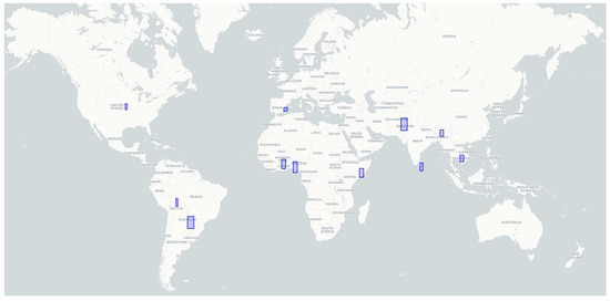
Figure 1.
Distribution of flood events highlighted in blue frames from the Sen1Floods11 dataset. Additional details are provided in Table S1.
Using the Sen1Floods11 dataset, the hand-labeled samples from 11 flood events were selected, with 8 events used for validation and 3 events reserved from testing. For each validation flood event, up to 300 SAR pixels for each land cover type were randomly selected to serve as training samples. These validation events, from which training samples were derived, occurred in geographically diverse locations, including Spain, Nigeria, Bolivia, India, Paraguay, Somalia, Sri Lanka, and the USA. The test events, without any samples collected, were situated in Ghana, Pakistan, and Cambodia to evaluate the method’s performance.
In this study, regions for applying local thresholds were defined based on homogeneous land use and land cover characteristics. To achieve this, discrete classes from the Copernicus Global Land Cover Layers (CGLS-LC100) Collection 3, a dataset offering a globally consistent 100 m resolution map for the period 2015–2019, were used [59]. It includes categories such as shrubs, herbaceous vegetation, agriculture, urban areas, bare ground, wetlands, closed forest (>70% tree canopy), and open forest (15–70% canopy). With around 80% accuracy at continental scales [60] and annual updates, this dataset allows for land-cover-specific thresholding applications.
2.2. Method
The SAR instrument measures radar backscatter from the ground, with signal intensity influenced by surface structure and roughness. Structurally complex targets, such as buildings and forests, reflect more radar signals, resulting in brighter features, while flat surfaces like calm water reflect the SAR signal away, leading to darker areas with low backscatter [24]. This contrast underpins our near-real-time inundation mapping, which applies local thresholds, land cover data, and preprocessed Sentinel-1 GRD imagery within Google Earth Engine (GEE).
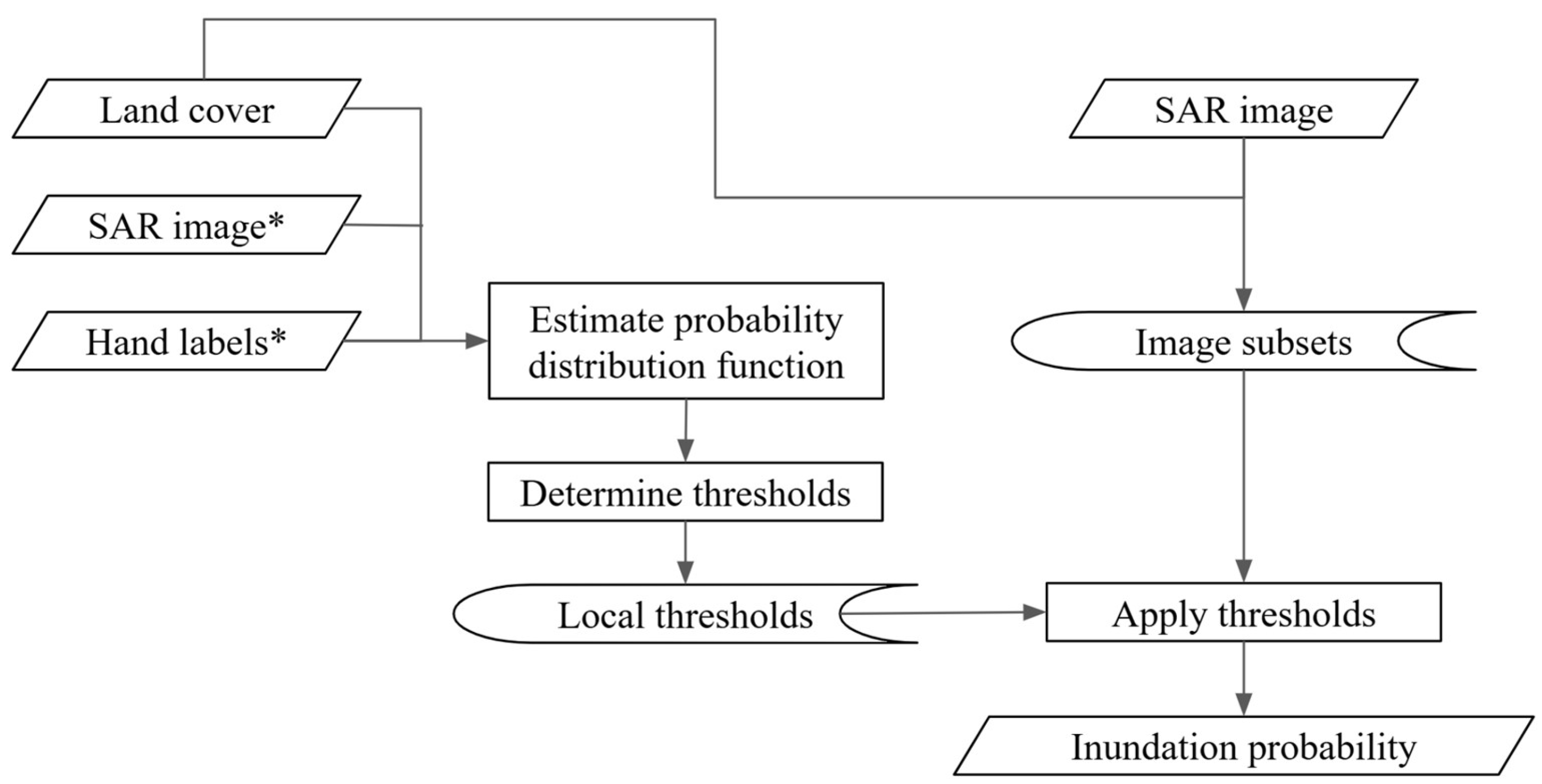
Our approach (Figure 2) draws stratified random samples of SAR backscatter with distinct land cover classes. We then fit gamma distributions for each polarization–land cover pair to derive probability thresholds; lower backscatter signifies higher likelihood of inundation. These thresholds are applied to the target SAR images, aggregating probabilities across all land covers to form comprehensive inundation maps. By capturing each land cover’s unique radar signature, this local-threshold approach enhances detection accuracy and reliability. It provides a robust framework for large-scale, near-real-time mapping, enabling more informed management and swifter response when floods occur.
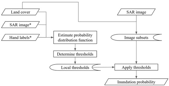
Figure 2.
Flowchart of the proposed local thresholding method (SAR image* and hand labels* are from the Sen1Floods11 dataset).
2.2.1. Extract Samples
The analysis started with the extraction of stratified random samples from the dataset’s training events across Bolivia (flooding happened on 15 February 2018), India (12 August 2016), Paraguay (31 October 2018), Nigeria (21 September 2018), Somalia (7 May 2018), Sri Lanka (30 May 2017), Spain (17 September 2019), and the USA (22 May 2019). For each event, up to 300-pixel samples were selected per distinct CGLS-LC100 land cover type. Each sample contained data on SAR dual-polarization backscatter intensities, land cover types, manually labeled classifications (water, non-water, and cloud), and an event index. This approach yielded a rich dataset spanning various geographic regions and land types, ensuring the method’s capacity to detect inundation accurately across heterogeneous conditions.
We performed stratified sampling and calculated the thresholds 10 times, generating about 20,000 samples each time. The sample numbers for individual events ranged from about 1600 to 3400. Through these experiments, we observed minimal variation in the calculated thresholds: an average standard deviation of 0.12 dB for VV and 0.13 for VH. We attribute this stability to the large sample sizes and diverse coverage, and the probabilistic method can benefit from consistent local thresholds for reliable and adaptable detection across varying environments.
2.2.2. Fit Gamma Distributions
The next step was to model the sampled backscatter intensity as a gamma distribution at one polarization of each cluster c—such as water , urban areas , …, and forest . Considering a cluster c–a homogeneous surface, the probability density function (PDF) is
where a is a shape parameter, b is a scale parameter, and is the gamma function. This PDF is defined in its standardized form for . To accommodate the negative values of , a location parameter (‘loc’) is introduced from the Python 3 package ‘scipy’.
2.2.3. Calculate Local Thresholds
The shape, scale, and location parameters obtained from the fitted gamma functions were used to calculate percentiles, which served as probability thresholds. These percentiles were determined by applying the percent point function (PPF), a method that identifies the value below which a specified percentage of observations in the distribution falls.
The cumulative distribution function (CDF) of the gamma distribution is calculated by integrating the PDF :
The percent point function (PPF), denoted as , for the gamma distribution, represents the value of at which the CDF equals a specified percentage p:
The gamma distribution does not have a simple closed-form expression for its percent point function (PPF); however, it can be computed numerically using Python’s ‘scipy.stats.gamma.fit’.
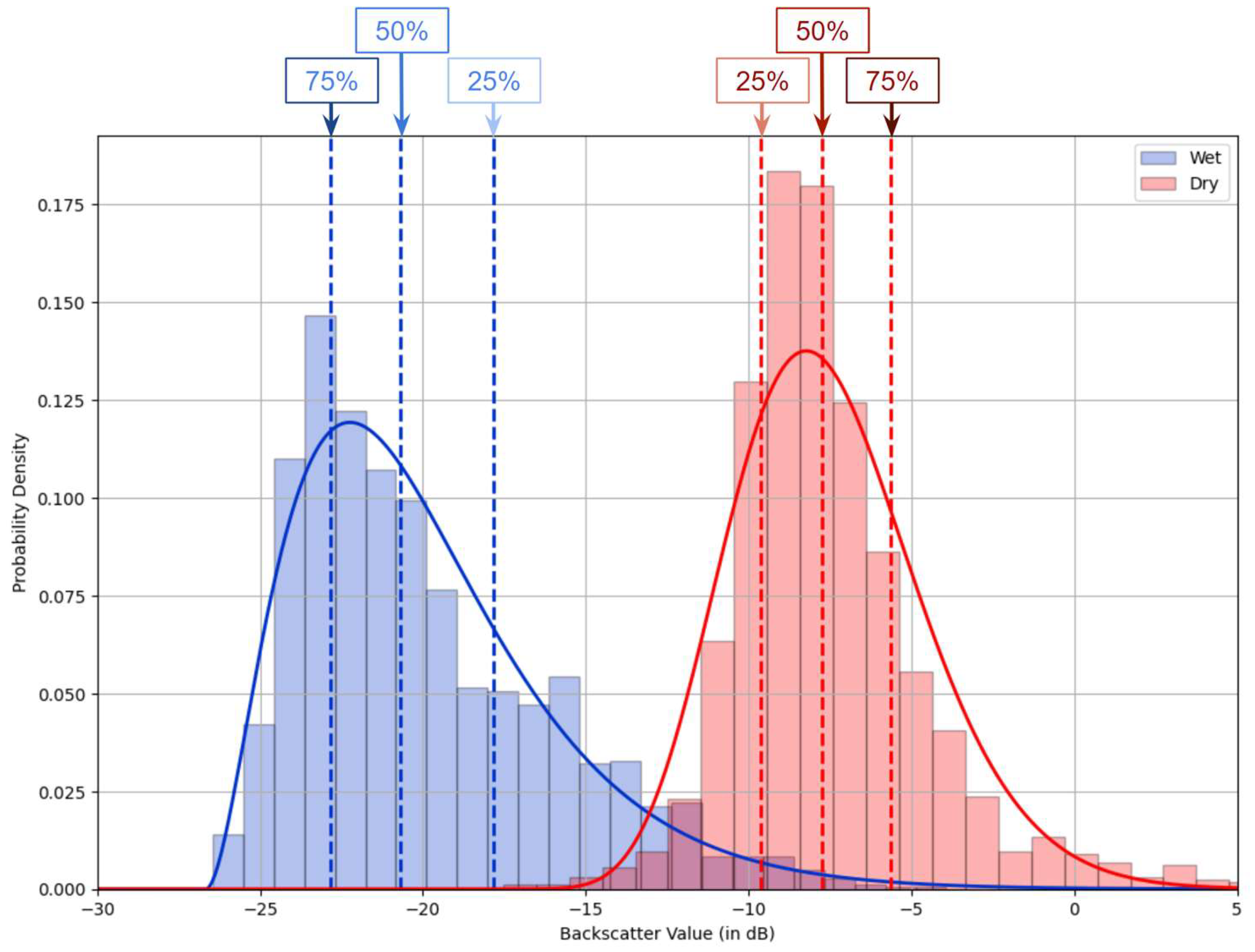
The PPF is a nondecreasing function, meaning that as the probability p increases, the value of does not decrease. In the context of SAR-based inundation detection, we calculate local thresholds using percentile-based lists that reflect the characteristics of SAR data. Specifically, lower backscatter values correlate with higher probabilities of being inundated (wet pixels), while higher backscatter values correspond to higher probabilities of being dry (dry pixels). This relationship is illustrated in Figure 3.

Figure 3.
Density distribution and derived thresholds illustrating the corresponding probabilities for wet (blue) and dry (red) pixels.
To systematically apply these thresholds, we used 19 percentiles (5th to 95th) in 5% increments, balancing computational efficiency and resolution. The resulting local threshold matrix consists of 19 percentile values × 2 polarizations (VV and VH), scaled by 9 land cover types (e.g., surface water, agriculture, urban areas, and forests). This structure ensures comprehensive SAR backscatter representation across different land cover categories.
2.2.4. Apply Local Thresholds on GEE
Thresholds of different probabilities, considering both polarizations and land cover types, are applied to the target SAR images. Pixels sharing the same polarization and land cover within an image are grouped and treated as a single local region (or an image subset). For each of these regions, backscatter values were compared to the thresholds derived for wet and dry probabilities at intervals of 5%, 10%, …, up to 95%.
To begin, we construct a Google Earth Engine image object containing a list of thresholds for each combination of polarization and land cover type. This object, threshold_wet, comprised a single image with 19 bands, where each band represents a threshold percentile value. We then apply these wet thresholds across the entire region using the efficient GEE function ee.Image.lt (threshold_wet). This function evaluates each pixel, returning a value of 1 if its SAR backscatter value falls below the corresponding wet threshold for the respective backscatter percentile (e.g., 5%, 10%, up to 95%). Next, we use the ee.Image.reduce (‘sum’) function to summarize the values across all bands at each pixel. This sum effectively indicates the level of wet probability associated with the SAR data. For instance, if the resulting pixel value is 15 (where 19 is the total number of thresholds, representing the maximum possible value for this pixel), it corresponds to a 75% probability of inundation.
For “dry” probabilities, the same principle applies but uses the ee.Image.gt (threshold_dry) function. Here, the backscatter value must exceed thresholds tailored to the remain-dry conditions. A pixel’s overall dryness probability is computed in a manner similar to the wet calculation. Finally, these wet and dry probabilities are compared: if the wet probability of a pixel is higher than its dry probability, the inundation map adopts the greater value as that pixel’s final flood likelihood. Because Sentinel-1 data include two polarizations, this process is run separately for each to preserve polarization-specific characteristics. The resulting probabilities from all subsets (different land covers and open-water classes) are then merged into a single comprehensive inundation probability map.
2.2.5. Accuracy Metrics
The primary output of our method is the calculation of inundation probabilities for each pixel within the SAR images. To effectively compare the actual binary outcomes (0 for non-surface water and 1 for surface water) with the estimated probabilities (discrete values of 0, 5%, 10%, …, 95%), it is essential to apply metrics that reflect the probabilistic nature. In this study, we utilized several key metrics and a visualizing tool, including the Brier Score [61], Logarithmic Loss [62], Expected Calibration Error (ECE) [63,64], and the Reliability Diagram [55,65].
The Brier Score is mathematically defined as
where represents the predicted inundation probability and denotes the actual outcome.
Logarithmic Loss further penalizes incorrect classifications as
The ECE quantifies the degree of miscalibration by calculating the weighted average of the differences using
Here, is the set of samples whose predicted probability falls within the m-th bin, represents the average accuracy, and is the average predicted probability. The weights, , correspond to the proportion of data points in each bin. Lower Brier Scores, Logarithmic Losses, or ECEs indicates better calibration, reflecting smaller discrepancies between predicted probabilities and observed frequencies.
3. Results
3.1. SAR Backscatter Distribution
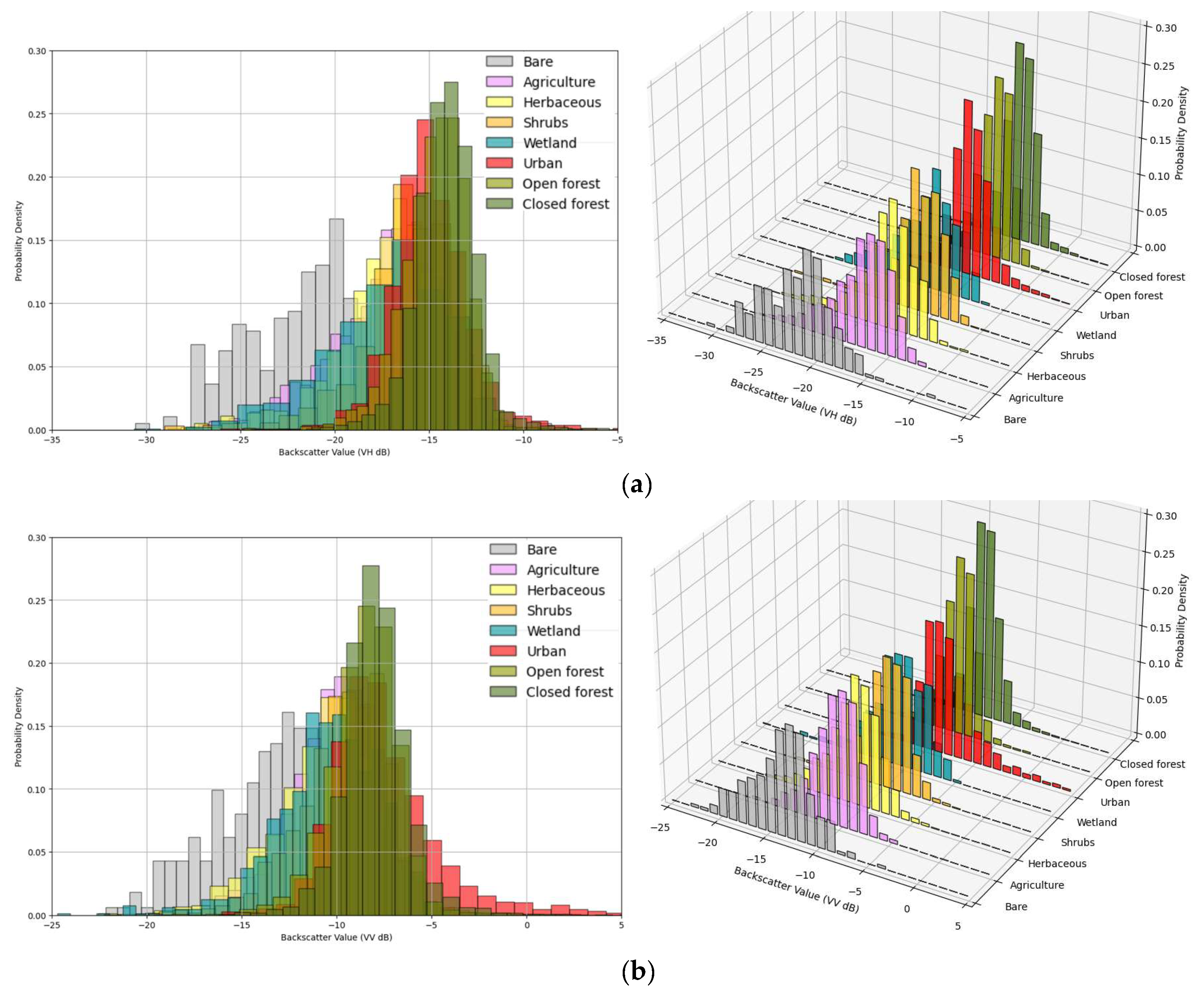
The following figure illustrates the density distribution of backscatter values across various land cover types under both dry and wet conditions. Figure 4a,b presents histograms of backscatter values for different dry land cover types, while Figure 4c focuses on inundated pixels. These histograms reveal distinct distributions among the land cover types. Generally, dry pixels exhibit higher backscatter intensities compared to wet pixels, with median backscatter values for forest pixels being higher than those for shrubs and herbaceous areas.

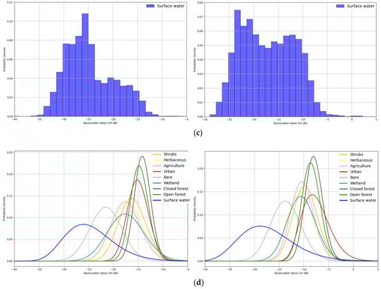
Figure 4.
Probability density histogram of sample backscatter (in dB) for different land covers and polarizations: (a) VH and (b) VV. The discrete classifications include bare, agriculture, herbaceous, shrubs, wetland, urban, open forest, and closed forest. The three-dimensional figures provide an alternative perspective. (c) Probability density histogram of the sample backscatter for inundation pixels (surface water) at two polarizations. (d) Fitted gamma distribution used to derive probabilistic thresholds for different land covers at two polarizations.
The distribution of land cover types across the eight validation events is uneven, and some land cover types are absent from certain flood events. If a particular land cover type is present in every validation event, it could yield 300 × 8 samples; in contrast, less common land cover types might contribute only a few samples. This variation in sample sizes necessitates combining data from multiple flood events to construct a comprehensive validation dataset.
In Figure 4d, the distributions were specific to each land cover type and polarization and were subsequently used to calculate probability thresholds. Surface water generally exhibits the lowest backscatter but the greatest variance, while forests—whether closed or open—and urban areas display consistently high backscatter with smaller variance. Bare areas, though similar to surface water regarding variance, have a higher median backscatter. The distributions for shrubs, agriculture, and wetlands overlapped yet remained distinct from those for water and bare land. Local thresholds were then derived using the percentage points of these probability distributions.
3.2. Accuracy Assessment
As shown in Table 1 and Table 2, the overall performance of the proposed method demonstrates satisfactory accuracy, namely the Brier Score (0.05–0.07), Logarithmic Loss (0.1–0.2), and Expected Calibration Error (0.03–0.04). These metrics indicate reliable performance in predicting inundation probabilities. For the validation events, the inundation probabilities derived from both VH and VV polarizations show comparable levels of accuracy. However, for the test events, where the sample data are unavailable, the method achieves better accuracy using VV polarization. This is particularly noticeable in the Logarithmic Loss values, where VV polarization achieves a lower value of 0.13 compared to 0.2 for VH polarization, suggesting that VV polarization provides more reliable inundation estimates in scenarios with limited data.

Table 1.
Accuracy assessment of the proposed method for validation and test events with thresholds derived from VH and VV polarizations.
Table 2.
Accuracy assessment of the proposed method across different land cover types for validation and test events with thresholds derived from VH and VV polarizations.
We observed large variations when examining the accuracy across different land cover types. Table 2 highlights that urban areas, closed forests, and open forest areas show strong performance, reflected in their low Brier Scores and Log Loss metrics. Conversely, inundation predictions in bare and wetland regions are less accurate. For instance, bare regions exhibit higher Brier Scores (0.18 for VH and 0.12 for VV) and Log Loss values (0.84 for VH and 0.62 for VV), indicating a greater mismatch between predicted and actual flood probabilities.
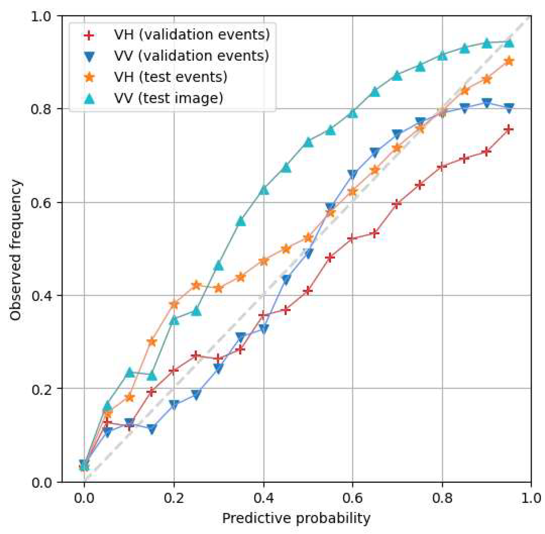
Reliability diagrams provide a visual comparison between predicted probabilities on the x-axis and actual outcomes (observed frequency) on the y-axis. Ideally, a well-calibrated model will produce a reliability diagram where the plotted points closely follow the diagonal line (y = x). Here, the predicted probabilities are binned into intervals of [0, 0.05), [0.05, 0.1), and so on. The average predicted probability and the observed frequency (occurrence of actual surface water pixels) are then calculated for each bin. These diagrams are useful for identifying specific areas of miscalibration, such as overestimated or underestimated probabilities in certain ranges.
The model’s predictive probabilities align closely with the observed frequencies for both validation and test events. Figure 5a shows that the VV points are positioned closer to the diagonal line, which indicates that VV polarization is more accurate in predicting inundation than the VH polarization. The VH bands tended to underestimate inundation probabilities, particularly in test events where no samples were collected.
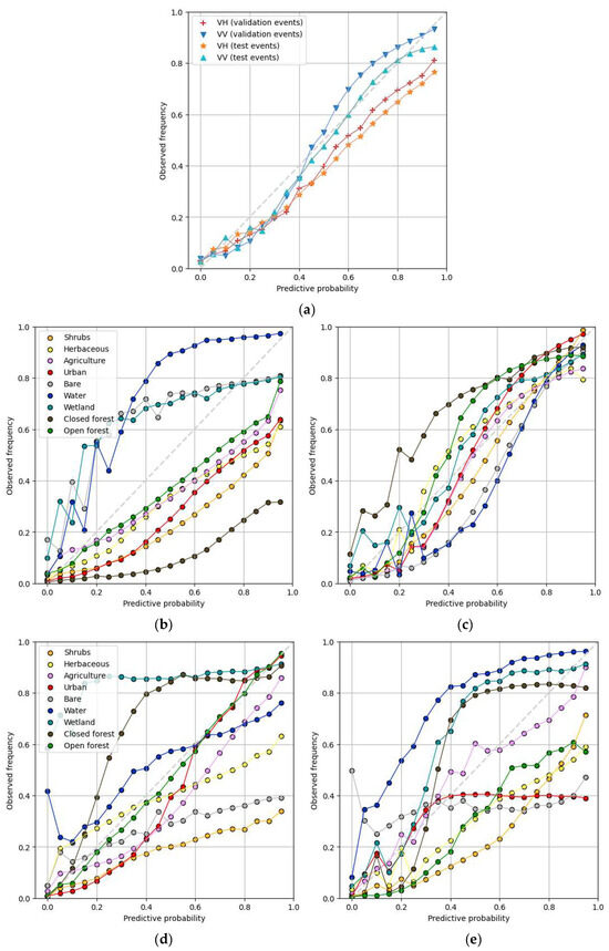
Figure 5.
(a) Reliability diagrams comparing predictive probability with observed frequency for validation and test events with VH and VV polarizations. Reliability diagrams for different land cover types in the validation (b,c) and test events (d,e), with VH (b,d) and VV (c,e) polarizations.
The reliability curves across different land cover types shows that higher predictive probabilities corresponded with higher observed wet pixel ratios (Figure 5b–e). However, when using the VH polarization (Figure 5b,d), land cover types such as bare land, water, and wetlands showed higher observed frequencies than the predicted probabilities, whereas closed forests and open forests exhibited lower observed frequencies. This suggests that detecting inundation in areas with dense vegetation, such as forests and shrubs, is more challenging when using the VH channels.
The reliability diagrams for the test events (Figure 5d,e) exhibited greater scatter compared to those for the validation events (Figure 5b,c). In urban areas, wetlands, and dense forests, the relationship between increases in estimated inundation probability and higher observed frequencies was weaker than in the validation events. Specifically, in urban areas, the local thresholds derived from VV data achieved only approximately 40% accuracy, despite showing a higher predictive probability.
3.3. Flood Event Image
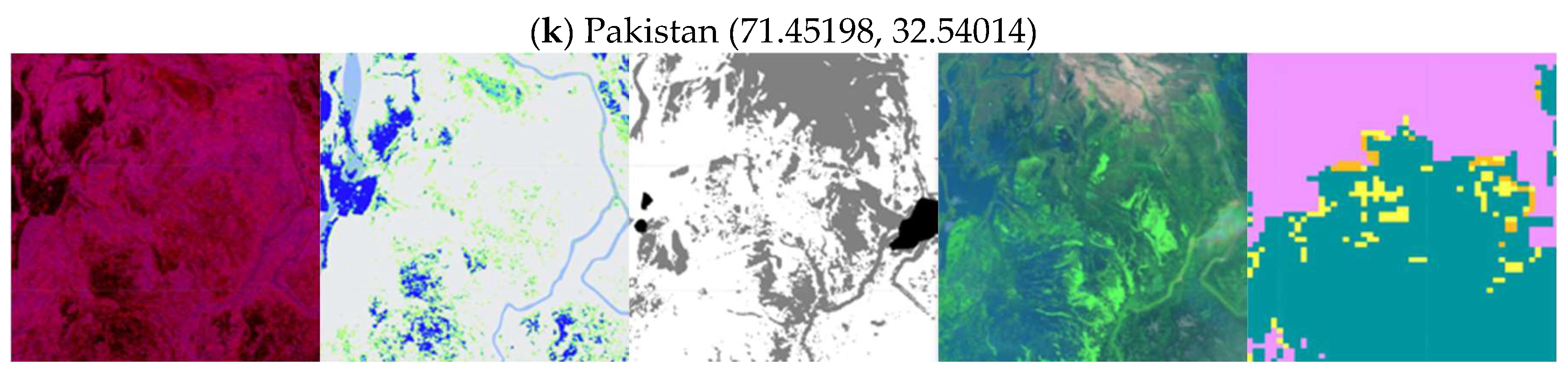
Figure 6 present the zoomed-in results from the validation and test events, accompanied by corresponding Sentinel-1 and Sentinel-2 images, hand-labeled classifications, and land cover types. The full coverage of the 11 flood events is available for exploration via the Supplementary Script. The below figures specifically highlight a zoomed-in area where the probabilistic inundation map (second column) is compared to the hand-labeled water areas (third column). The predictive water areas, marked with high probabilities in blue and low probabilities in green, align well with the hand-labeled areas shown in white.
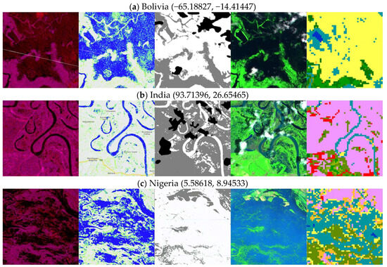
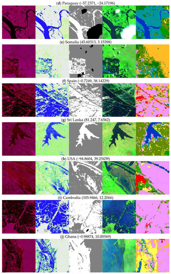

Figure 6.
Zoom-in regions within the validation events in (a) Bolivia, (b) India, (c) Nigeria, (d) Paraguay, (e) Somalia, (f) Spain, (g) Sri Lanka, (h) the USA, (i) Cambodia, (j) Ghana, and (k) Pakistan. From left to right: Sentinel-1 image (first column, red—VV, green—VH), estimated inundation probability (second column, green—low probability,  blue—high probability), the hand-labeled classification from Sen1floods11 (third column, white—surface water, gray—land, black—cloud or shadows), Sentinel-2 image (fourth column), and the land use and land cover map (fifth column, color as per CGLS-LC100).
blue—high probability), the hand-labeled classification from Sen1floods11 (third column, white—surface water, gray—land, black—cloud or shadows), Sentinel-2 image (fourth column), and the land use and land cover map (fifth column, color as per CGLS-LC100).
In most regions of Figure 6, the predicted water areas, depicted in blue, generally align with the hand-labeled water areas shown in white, although the alignment varies across locations. Bolivia (a) and India (b) demonstrate a closer match between the estimated and observed water areas, while Nigeria (c) exhibits more discrepancies, likely due to the more challenging environmental conditions present in that region. Specifically, Figure 6c highlights the presence of herbaceous wetlands, where a mixture of water and herbaceous or woody vegetation may complicate accurate predictions. Despite these challenges, the long, curving water bodies in the second column align closely with the white hand-labeled pixels in the third column. Similarly, Paraguay (d) shows strong alignment, particularly around the river areas.
The regions in Spain (f) and Sri Lanka (g) demonstrate strong alignment between the predicted (blue) and actual (white) water areas. In Spain (f), where agricultural areas are interspersed with urban land, the blue water areas in the inundation map closely correspond with the white hand-labeled areas. In contrast, Somalia (e) exhibits more discrepancies, with predicted water areas failing to align as well with the observed hand-labeled water areas. In particular, inundation areas with lower probability, situated around high-probability inundated zones, tend to be underestimated. The USA (h) shows reasonable alignment, especially around prominent water bodies and floodplain features. However, the model tends to underestimate inundation at the edges of these water bodies.
For the test events, Cambodia (i) exhibits the strongest alignment, with the predicted water areas closely matching the actual hand-labeled water areas. In contrast, Ghana (j) and Pakistan (k) display greater variability, primarily characterized by the method’s underestimation of water areas. These discrepancies indicate potential challenges in regions dominated by herbaceous vegetation, which consists of plants without persistent stems or firm structures, and where tree and shrub cover is less than 10%. Similar challenges are observed in herbaceous wetlands.
4. Discussion
4.1. Flood Detection
Inundation mapping is essential for flood response but often lacks the specificity required for rapid decision-making. While it identifies both permanent water bodies and flood-induced submersion, flood mapping focuses solely on regions that become inundated due to an event. To enhance detection, probabilistic methods leverage temporal backscatter anomalies and statistical analysis, as proposed by DeVries et al. (2020) [57]. This approach utilizes two key strategies: (1) continuously mapping inundation probability over time and (2) comparing recent SAR-derived probabilities against a baseline map, where increases indicate flooding.
A reliable baseline is crucial but challenging due to spatial and temporal variability in surface water distribution. Sentinel-1 SAR data can establish this baseline using annual statistics that reflect typical (non-flood) conditions. By applying median pre-event images, as demonstrated by Singha et al. (2020) [40], and measuring probability increases, flood mapping accuracy improves. Reliability diagrams (Figure 7) show that this method aligns closely with single-event image-based mapping.
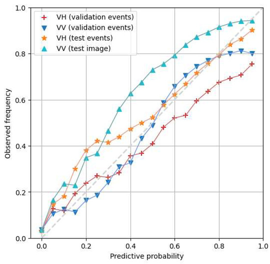
Figure 7.
Reliability diagrams comparing predictive probability with observed frequency for validation and test events with two polarizations (VH and VV) and both pre- and post-flood images, where the pre-flood image represents the annual median before the flood events.
A comparison in Table 3 between DeVries’s method and the proposed approach reveals notable differences. While DeVries’s method provides a relatively uniform prediction ratio across probability levels (e.g., 0.41 for low and 0.35 for median), the local thresholding method captures more detailed variations, offering better differentiation across probability ranges. Furthermore, the number of accurately predicted flooded pixels using DeVries’s method (1,264,608) is substantially smaller than those identified by local thresholding (2,086,250 from VH and 2,513,816 from VV), representing 65% and 98% increases in correct labels from local thresholding, across all probability levels—low, median, and high.
Table 3.
Comparison of accuracy between DeVries et al. (2020)’s method and the proposed local thresholding method across low, median, and high probability ranges. The predictions by DeVries et al. (2020) were obtained using their published GEE script. For comparison, local thresholding estimates were categorized as follows: low probability (p < 0.35), median probability (0.35 ≤ p ≤ 0.65), and high probability (p > 0.65). The table presents the number of hand-labeled flooded pixels (Label), predicted flooded pixels (Prediction), and the ratio of label to prediction (Ratio) for each method at different probability levels.
One major advantage of local thresholding is its broader coverage of flood-prone areas, making it especially useful for large-scale assessments, disaster response, and early warnings. This comprehensive mapping ensures that critical flooded regions, particularly in rural or remote areas, are not overlooked. However, this increased detection capability comes at the cost of a higher false-positive rate, highlighting the trade-off between accuracy and coverage.
4.2. Limitation and Future Direction
Inundation mapping with SAR images faces several challenges affecting accuracy and reliability. A key limitation is radar backscatter variability, influenced by target characteristics, sensor specifications, and observation geometry. Speckle noise, a granular distortion inherent to SAR imaging can cause unrealistic inundation probability maps. Postprocessing techniques, such as computer vision algorithms and additional datasets like Height Above Nearest Drainage (HAND), can help refine results by integrating elevation data and streamflow inputs [35,66,67,68].
Another limitation is SAR’s sensitivity to the projected local incidence angle (PLIA, θ), which affects backscatter intensity. As θ increases, less energy returns to the sensor, leading to variability in inundation probability predictions. This dependency is particularly pronounced in topographically complex areas [69]. Vegetation further complicates backscatter interpretation due to volume scattering. Future improvements could refine θ-backscatter modeling and incorporate higher-resolution DEMs for better terrain correction.
Noise artifacts in SAR images present additional challenges, especially at image borders and along-track edges [70]. Addressing these artifacts is crucial for accurate flood extent analysis across mosaicked datasets. Additionally, Sentinel-1’s relatively low temporal resolution limits data availability for estimating flood duration, economic losses, and short-duration event dynamics [71,72]. Despite these constraints, probabilistic inundation maps offer valuable applications, including flood extent delineation, depth estimation [73], and improved hydraulic modeling for flood risk assessments [74]. Addressing these limitations will enhance the reliability and applicability of SAR-based flood mapping across diverse scenarios.
While our probabilistic local thresholding approach demonstrated performance and operational scalability, we recognize several intrinsic limitations for future research. The method’s lower accuracy in bare and wetland regions reflects SAR backscatter ambiguities, suggesting the potential of integrating auxiliary datasets such as LiDAR, HAND, or refined land cover classifications as promising future directions to enhance detection accuracy. Additionally, Sentinel-1’s revisit interval can limit the detection of short-duration floods; incorporating data from higher-frequency missions or optical sensors during cloud-free conditions could significantly narrow these temporal gaps. Similarly, the use of finer-resolution land cover datasets could improve local thresholding by more accurately capturing land surface heterogeneity. Moreover, although the gamma distribution generally provides robust performance, our analysis identified notable discrepancies in specific scenarios. These findings explicitly highlight the potential value of exploring hybrid distributions in future studies to further enhance local threshold accuracy and robustness in complex land cover environments. The current validation, based on the Sen1Floods11 dataset, may not represent all flood types, particularly urban flash floods, snowmelt-driven inundation, and coastal surges. Expanding validation to include these scenarios and leveraging independent ground truth sources such as UAV or gauge measurements would bolster reliability. Lastly, explicitly quantifying the uncertainty propagated from land cover misclassifications and developing interactive visualization tools are important future enhancements to improve confidence in classification results and flood risk communication for decision-makers. Addressing these points in subsequent studies can strengthen the adaptability and operational robustness of SAR-based probabilistic inundation mapping.
The proposed method is inherently flexible and adaptable to diverse geographies and evolving data environments. By providing pixel-level inundation probabilities rather than fixed classifications, it allows users to define custom thresholds based on their specific operational needs or risk tolerances. This adaptability is particularly valuable in complex or noisy environments—such as heterogeneous landscapes, transitional flood zones, or areas with frequent cloud cover—where deterministic classification may fail to capture subtle variations in inundation signals. Importantly, the local thresholding framework is designed to be modular: thresholds can be updated or recalibrated with new training data as additional flood events occur or as more accurate land cover information becomes available. This capability ensures that the model remains responsive to spatial, temporal, or environmental changes, enhancing its applicability for operational use in new regions or under shifting hydrological conditions. As such, the method supports not only initial implementation but also ongoing refinement by planners, emergency responders, and analysts working in diverse and data-scarce settings.
5. Conclusions
This study introduces a rapid probabilistic inundation mapping method leveraging local thresholding of Sentinel-1 SAR imagery, implemented efficiently on the Google Earth Engine (GEE) platform. Unlike traditional deterministic inundation mapping approaches, which offer binary outcomes, our probabilistic framework quantifies inundation likelihood at the pixel level, explicitly representing uncertainties inherent in flood detection. Firstly, we developed a scalable, near-real-time inundation mapping method utilizing Sentinel-1 SAR data, optimized through local thresholds tailored to specific land cover types. Our validation, using the globally diverse Sen1Floods11 dataset covering flood events across five continents, suggests the approach’s generalizability, effective calibration, and predictive accuracy.
Secondly, this study explored polarization-specific performance, clearly demonstrating that VV polarization (vertical transmit, vertical receive) outperformed VH polarization, particularly in challenging environments lacking adequate sample data. The superior sensitivity of VV polarization to surface roughness and structures makes it especially suitable for identifying inundation in urbanized or vegetated regions. Thirdly, significant variability in model accuracy across different land cover types was identified, with high performance in urban and forested areas contrasted by relatively lower accuracy in bare and wetland regions. These disparities highlight intrinsic SAR backscatter ambiguities that complicate inundation detection, underscoring the necessity for integrating auxiliary data to enhance accuracy.
Furthermore, we compared our local thresholding method against established techniques, demonstrating improvements in identifying flooded pixels across various inundation probabilities. This enhanced detection capability is particularly beneficial for comprehensive large-scale flood assessments, providing critical information for rapid emergency responses. Finally, the methodological flexibility inherent in our probabilistic approach allows for continuous refinement and adaptation to evolving datasets, land cover changes, and specific operational contexts. Future research directions highlighted include the integration of high-resolution auxiliary datasets, incorporation of temporal baseline imagery, machine learning, and cross-validation using independent ground truth measurements. Such enhancements will improve inundation detection accuracy, reduce temporal observation gaps, and better quantify uncertainties stemming from land cover misclassification. Overall, our proposed method offers a valuable advancement in operational flood risk assessment, significantly enhancing the accuracy, interpretability, and operational applicability of SAR-based inundation mapping.
Supplementary Materials
The following supporting information can be downloaded at: https://www.mdpi.com/article/10.3390/rs17101747/s1, Table S1: The 11 flood event locations used in this study [48].
Author Contributions
Conceptualization and methodology, J.L., D.L. and K.H.; software and validation, J.L. and L.F.; writing—original draft preparation, J.L.; writing—review and editing, visualization, J.L., D.L., L.F. and K.H.; funding acquisition, J.L. All authors have read and agreed to the published version of the manuscript.
Funding
This research was funded by the Shanghai Pujiang Program, grant number 23PJ1410100 STCSM.
Data Availability Statement
The original contributions presented in this study are included in the article/Supplementary Materials. Further inquiries can be directed to the corresponding author.
Conflicts of Interest
The authors declare no conflicts of interest. The funders had no role in the design of this study; in the collection, analyses, or interpretation of the data; in the writing of the manuscript; or in the decision to publish the results.
References
- Rentschler, J.; Salhab, M.; Jafino, B.A. Flood exposure and poverty in 188 countries. Nat. Commun. 2022, 13, 3527. [Google Scholar] [CrossRef] [PubMed]
- Tellman, B.; Sullivan, J.A.; Kuhn, C.; Kettner, A.J.; Doyle, C.S.; Brakenridge, G.R.; Erickson, T.A.; Slayback, D.A. Satellite imaging reveals increased proportion of population exposed to floods. Nature 2021, 596, 80–86. [Google Scholar] [CrossRef]
- Tiggeloven, T.; de Moel, H.; Winsemius, H.C.; Eilander, D.; Erkens, G.; Gebremedhin, E.; Loaiza, A.D.; Kuzma, S.; Luo, T.Y.; Iceland, C.; et al. Global-scale benefit-cost analysis of coastal flood adaptation to different flood risk drivers using structural measures. Nat. Hazards Earth Syst. Sci. 2020, 20, 1025–1044. [Google Scholar] [CrossRef]
- Tebaldi, C.; Ranasinghe, R.; Vousdoukas, M.; Rasmussen, D.J.; Vega-Westhoff, B.; Kirezci, E.; Kopp, R.E.; Sriver, R.; Mentaschi, L. Extreme sea levels at different global warming levels. Nat. Clim. Change 2021, 11, 746–751. [Google Scholar] [CrossRef]
- Andreadis, K.M.; Wing, O.E.J.; Colven, E.; Gleason, C.J.; Bates, P.D.; Brown, C.M. Urbanizing the floodplain: Global changes of imperviousness in flood-prone areas. Environ. Res. Lett. 2022, 17, 104024. [Google Scholar] [CrossRef]
- Paprotny, D.; Mengel, M. Population, land use and economic exposure estimates for Europe at 100 m resolution from 1870 to 2020. Sci. Data 2023, 10, 372. [Google Scholar] [CrossRef]
- Rajib, A.; Zheng, Q.J.; Lane, C.R.; Golden, H.E.; Christensen, J.R.; Isibor, I.I.; Johnson, K. Human alterations of the global floodplains 1992–2019. Sci. Data 2023, 10, 499. [Google Scholar] [CrossRef] [PubMed]
- Kulp, S.A.; Strauss, B.H. New elevation data triple estimates of global vulnerability to sea-level rise and coastal flooding. Nat. Commun. 2019, 10, 4844. [Google Scholar] [CrossRef]
- Strauss, B.H.; Kulp, S.A.; Rasmussen, D.J.; Levermann, A. Unprecedented threats to cities from multi-century sea level rise. Environ. Res. Lett. 2021, 16, 114015. [Google Scholar] [CrossRef]
- Hirabayashi, Y.; Tanoue, M.; Sasaki, O.; Zhou, X.D.; Yamazaki, D. Global exposure to flooding from the new CMIP6 climate model projections. Sci. Rep. 2021, 11, 3740. [Google Scholar] [CrossRef]
- Trigg, M.A.; Birch, C.E.; Neal, J.C.; Bates, P.D.; Smith, A.; Sampson, C.C.; Yamazaki, D.; Hirabayashi, Y.; Pappenberger, F.; Dutra, E.; et al. The credibility challenge for global fluvial flood risk analysis. Environ. Res. Lett. 2016, 11, 094014. [Google Scholar] [CrossRef]
- CRED. 2021 Disasters in Numbers; Centre for Research on the Epidemiology of Disasters (CRED): Brussels, Belgium, 2022. [Google Scholar]
- Hemmati, M.; Mahmoud, H.N.; Ellingwood, B.R.; Crooks, A.T. Shaping urbanization to achieve communities resilient to floods. Environ. Res. Lett. 2021, 16, 094033. [Google Scholar] [CrossRef]
- Jones, R.L.; Guha-Sapir, D.; Tubeuf, S. Human and economic impacts of natural disasters: Can we trust the global data? Sci. Data 2022, 9, 572. [Google Scholar] [CrossRef]
- Malenovsky, Z.; Rott, H.; Cihlar, J.; Schaepman, M.E.; García-Santos, G.; Fernandes, R.; Berger, M. Sentinels for science: Potential of Sentinel-1, -2, and -3 missions for scientific observations of ocean, cryosphere, and land. Remote Sens. Environ. 2012, 120, 91–101. [Google Scholar] [CrossRef]
- Voigt, S.; Giulio-Tonolo, F.; Lyons, J.; Kucera, J.; Jones, B.; Schneiderhan, T.; Platzeck, G.; Kaku, K.; Hazarika, M.K.; Czaran, L.; et al. Global trends in satellite-based emergency mapping. Science 2016, 353, 247–252. [Google Scholar] [CrossRef] [PubMed]
- Manavalan, R. SAR image analysis techniques for flood area mapping—Literature survey. Earth Sci. Inform. 2017, 10, 1–14. [Google Scholar] [CrossRef]
- Torres, R.; Snoeij, P.; Geudtner, D.; Bibby, D.; Davidson, M.; Attema, E.; Potin, P.; Rommen, B.; Floury, N.; Brown, M.; et al. GMES Sentinel-1 mission. Remote Sens. Environ. 2012, 120, 9–24. [Google Scholar] [CrossRef]
- D'Addabbo, A.; Refice, A.; Pasquariello, G.; Lovergine, F.P.; Capolongo, D.; Manfreda, S. A Bayesian Network for Flood Detection Combining SAR Imagery and Ancillary Data. IEEE Trans. Geosci. Remote Sens. 2016, 54, 3612–3625. [Google Scholar] [CrossRef]
- Nico, G.; Pappalepore, M.; Pasquariello, G.; Refice, A.; Samarelli, S. Comparison of SAR amplitude vs. coherence flood detection methods—A GIS application. Int. J. Remote Sens. 2000, 21, 1619–1631. [Google Scholar] [CrossRef]
- Plank, S.; Jüssi, M.; Martinis, S.; Twele, A. Mapping of flooded vegetation by means of polarimetric Sentinel-1 and ALOS-2/PALSAR-2 imagery. Int. J. Remote Sens. 2017, 38, 3831–3850. [Google Scholar] [CrossRef]
- Refice, A.; Capolongo, D.; Lepera, A.; Pasquariello, G.; Pietranera, L.; Volpec, F. SAR and InSAR for Flood Monitoring: Examples With COSMO-SkyMed Data. IEEE J. Sel. Top. Appl. Earth Obs. Remote Sens. 2014, 7, 2711–2722. [Google Scholar] [CrossRef]
- Zhang, X.; Jones, C.E.; Oliver-Cabrera, T.; Simard, M.; Fagherazzi, S. Using rapid repeat SAR interferometry to improve hydrodynamic models of flood propagation in coastal wetlands. Adv. Water Resour. 2022, 159, 104088. [Google Scholar] [CrossRef]
- Bauer-Marschallinger, B.; Cao, S.M.; Navacchi, C.; Freeman, V.; Reuss, F.; Geudtner, D.; Rommen, B.; Vega, F.C.; Snoeij, P.; Attema, E.; et al. The normalised Sentinel-1 Global Backscatter Model, mapping Earth’s land surface with C-band microwaves. Sci. Data 2021, 8, 277. [Google Scholar] [CrossRef]
- Chini, M.; Hostache, R.; Giustarini, L.; Matgen, P. A Hierarchical Split-Based Approach for Parametric Thresholding of SAR Images: Flood Inundation as a Test Case. IEEE Trans. Geosci. Remote Sens. 2017, 55, 6975–6988. [Google Scholar] [CrossRef]
- Cian, F.; Marconcini, M.; Ceccato, P. Normalized Difference Flood Index for rapid flood mapping: Taking advantage of EO big data. Remote Sens. Environ. 2018, 209, 712–730. [Google Scholar] [CrossRef]
- Ety, N.J.; Chu, Z.; Masum, S.M. Monitoring of flood water propagation based on microwave and optical imagery. Quatern. Int. 2021, 574, 137–145. [Google Scholar] [CrossRef]
- Kuenzer, C.; Guo, H.D.; Huth, J.; Leinenkugel, P.; Li, X.W.; Dech, S. Flood Mapping and Flood Dynamics of the Mekong Delta: ENVISAT-ASAR-WSM Based Time Series Analyses. Remote Sens. 2013, 5, 687–715. [Google Scholar] [CrossRef]
- Long, S.; Fatoyinbo, T.E.; Policelli, F. Flood extent mapping for Namibia using change detection and thresholding with SAR. Environ. Res. Lett. 2014, 9, 035002. [Google Scholar] [CrossRef]
- Manjusree, P.; Kumar, L.P.; Bhatt, C.M.; Rao, G.S.; Bhanumurthy, V. Optimization of Threshold Ranges for Rapid Flood Inundation Mapping by Evaluating Backscatter Profiles of High Incidence Angle SAR Images. Int. J. Disaster Risk Sci. 2012, 3, 113–122. [Google Scholar] [CrossRef]
- Markert, K.N.; Chishtie, F.; Anderson, E.R.; Saah, D.; Griffin, R.E. On the merging of optical and SAR satellite imagery for surface water mapping applications. Results Phys. 2018, 9, 275–277. [Google Scholar] [CrossRef]
- Moser, G.; Serpico, S.B. Generalized minimum-error thresholding for unsupervised change detection from SAR amplitude imagery. IEEE Trans. Geosci. Remote Sens. 2006, 44, 2972–2982. [Google Scholar] [CrossRef]
- Schlaffer, S.; Matgen, P.; Hollaus, M.; Wagner, W. Flood detection from multi-temporal SAR data using harmonic analysis and change detection. Int. J. Appl. Earth Obs. 2015, 38, 15–24. [Google Scholar] [CrossRef]
- Tong, X.H.; Luo, X.; Liu, S.G.; Xie, H.; Chao, W.; Liu, S.; Liu, S.J.; Makhinov, A.N.; Makhinova, A.F.; Jiang, Y.Y. An approach for flood monitoring by the combined use of Landsat 8 optical imagery and COSMO-SkyMed radar imagery. ISPRS J. Photogramm. Remote. Sens. Remote. Sens. 2018, 136, 144–153. [Google Scholar] [CrossRef]
- Twele, A.; Cao, W.X.; Plank, S.; Martinis, S. Sentinel-1-based flood mapping: A fully automated processing chain. Int. J. Remote Sens. 2016, 37, 2990–3004. [Google Scholar] [CrossRef]
- White, L.; Brisco, B.; Dabboor, M.; Schmitt, A.; Pratt, A. A Collection of SAR Methodologies for Monitoring Wetlands. Remote Sens. 2015, 7, 7615–7645. [Google Scholar] [CrossRef]
- Huang, W.L.; DeVries, B.; Huang, C.Q.; Lang, M.W.; Jones, J.W.; Creed, I.F.; Carroll, M.L. Automated Extraction of Surface Water Extent from Sentinel-1 Data. Remote Sens. 2018, 10, 797. [Google Scholar] [CrossRef]
- Martinis, S.; Kersten, J.; Twele, A. A fully automated TerraSAR-X based flood service. ISPRS J. Photogramm. Remote. Sens. Remote. Sens. 2015, 104, 203–212. [Google Scholar] [CrossRef]
- Pulvirenti, L.; Pierdicca, N.; Chini, M.; Guerriero, L. An algorithm for operational flood mapping from Synthetic Aperture Radar (SAR) data using fuzzy logic. Nat. Hazards Earth Syst. Sci. 2011, 11, 529–540. [Google Scholar] [CrossRef]
- Singha, M.; Dong, J.W.; Sarmah, S.; You, N.S.; Zhou, Y.; Zhang, G.L.; Doughty, R.; Xiao, X.M. Identifying floods and flood-affected paddy rice fields in Bangladesh based on Sentinel-1 imagery and Google Earth Engine. ISPRS J. Photogramm. Remote. Sens. 2020, 166, 278–293. [Google Scholar] [CrossRef]
- Amitrano, D.; Di Martino, G.; Iodice, A.; Riccio, D.; Ruello, G. Unsupervised Rapid Flood Mapping Using Sentinel-1 GRD SAR Images. IEEE Trans. Geosci. Remote. Sens. 2018, 56, 3290–3299. [Google Scholar] [CrossRef]
- Clement, M.A.; Kilsby, C.G.; Moore, P. Multi-temporal synthetic aperture radar flood mapping using change detection. J. Flood Risk Manag. 2018, 11, 152–168. [Google Scholar] [CrossRef]
- Hostache, R.; Matgen, P.; Wagner, W. Change detection approaches for flood extent mapping: How to select the most adequate reference image from online archives? Int. J. Appl. Earth Obs. 2012, 19, 205–213. [Google Scholar] [CrossRef]
- Lu, J.; Li, J.; Chen, G.; Zhao, L.J.; Xiong, B.L.; Kuang, G.Y. Improving Pixel-Based Change Detection Accuracy Using an Object-Based Approach in Multitemporal SAR Flood Images. IEEE J. Sel. Top. Appl. Earth Obs. Remote. Sens. 2015, 8, 3486–3496. [Google Scholar] [CrossRef]
- Mason, D.C.; Giustarini, L.; Garcia-Pintado, J.; Cloke, H.L. Detection of flooded urban areas in high resolution Synthetic Aperture Radar images using double scattering. Int. J. Appl. Earth Obs. 2014, 28, 150–159. [Google Scholar] [CrossRef]
- Debusscher, B.; Van Coillie, F. Object-Based Flood Analysis Using a Graph-Based Representation. Remote Sens. 2019, 11, 1883. [Google Scholar] [CrossRef]
- Mason, D.C.; Speck, R.; Devereux, B.; Schumann, G.J.P.; Neal, J.C.; Bates, P.D. Flood Detection in Urban Areas Using TerraSAR-X. IEEE Trans. Geosci. Remote. Sens. 2010, 48, 882–894. [Google Scholar] [CrossRef]
- Bonafilia, D.; Tellman, B.; Anderson, T.; Issenberg, E. Sen1Floods11: A georeferenced dataset to train and test deep learning flood algorithms for Sentinel-1. In Proceedings of the 2020 IEEE/CVF Conference on Computer Vision and Pattern Recognition Workshops (CVPRW), Seattle, WA, USA, 14–19 June 2020; pp. 835–845. [Google Scholar] [CrossRef]
- Liu, B.; Li, X.F.; Zheng, G. Coastal Inundation Mapping From Bitemporal and Dual-Polarization SAR Imagery Based on Deep Convolutional Neural Networks. J. Geophys. Res. Oceans 2019, 124, 9101–9113. [Google Scholar] [CrossRef]
- Muñoz, D.F.; Muñoz, P.; Moftakhari, H.; Moradkhani, H. From local to regional compound flood mapping with deep learning and data fusion techniques. Sci. Total Environ. 2021, 782, 146927. [Google Scholar] [CrossRef]
- Otsu, N. Threshold Selection Method from Gray-Level Histograms. IEEE Trans. Syst. Man Cybern. 1979, 9, 62–66. [Google Scholar] [CrossRef]
- Liang, J.Y.; Liu, D.S. A local thresholding approach to flood water delineation using Sentinel-1 SAR imagery. ISPRS J. Photogramm. Remote. Sens. 2020, 159, 53–62. [Google Scholar] [CrossRef]
- Jafarzadegan, K.; Abbaszadeh, P.; Moradkhani, H. Sequential data assimilation for real-time probabilistic flood inundation mapping. Hydrol. Earth Syst. Sci. 2021, 25, 4995–5011. [Google Scholar] [CrossRef]
- Westerhoff, R.S.; Kleuskens, M.P.H.; Winsemius, H.C.; Huizinga, H.J.; Brakenridge, G.R.; Bishop, C. Automated global water mapping based on wide-swath orbital synthetic-aperture radar. Hydrol. Earth Syst. Sci. 2013, 17, 651–663. [Google Scholar] [CrossRef]
- Schlaffer, S.; Chini, M.; Giustarini, L.; Matgen, P. Probabilistic mapping of flood-induced backscatter changes in SAR time series. Int. J. Appl. Earth Obs. 2017, 56, 77–87. [Google Scholar] [CrossRef]
- Gorelick, N.; Hancher, M.; Dixon, M.; Ilyushchenko, S.; Thau, D.; Moore, R. Google Earth Engine: Planetary-scale geospatial analysis for everyone. Remote Sens. Environ. 2017, 202, 18–27. [Google Scholar] [CrossRef]
- DeVries, B.; Huang, C.Q.; Armston, J.; Huang, W.L.; Jones, J.W.; Lang, M.W. Rapid and robust monitoring of flood events using Sentinel-1 and Landsat data on the Google Earth Engine. Remote Sens. Environ. 2020, 240, 111664. [Google Scholar] [CrossRef]
- Hamidi, E.; Peter, B.G.; Muñoz, D.F.; Moftakhari, H.; Moradkhani, H. Fast Flood Extent Monitoring with SAR Change Detection Using Google Earth Engine. IEEE Trans. Geosci. Remote. Sens. 2023, 61, 4201419. [Google Scholar] [CrossRef]
- Buchhorn, M.; Bertels, L.; Smets, B.; De Roo, B.; Lesiv, M.; Tsendbazar, N.E.; Masiliunas, D.; Linlin, L. Copernicus Global Land Service: Land Cover 100 m: Version 3 Globe 2015–2019: Algorithm Theoretical Basis Document; Zenodo: Geneve, Switzerland, 2020. [Google Scholar] [CrossRef]
- Tsendbazar, N.E.; Tarko, A.; Linlin, L.; Herold, M.; Lesiv, M.; Fritz, S.; Maus, V. Copernicus Global Land Service: Land Cover 100 m: Version 3 Globe 2015–2019: Validation Report; Zenodo: Geneve, Switzerland, 2020. [Google Scholar] [CrossRef]
- Brier, G.W. Verification of forecasts expressed in terms of probability. Mon. Weather. Rev. 1950, 78, 1–3. [Google Scholar] [CrossRef]
- Good, I.J. Rational decisions. J. R. Stat. Soc. Ser. B (Methodol.) 1952, 14, 107–114. [Google Scholar] [CrossRef]
- Morris, H.; DeGroot, S.E.F. The comparison and evaluation of forecasters. J. R. Stat. Soc. Ser. D (Stat.) 1983, 32, 12–22. [Google Scholar]
- Nicolas Posocco, A.B. Estimating Expected Calibration Errors. In Proceedings of the Artificial Neural Networks and Machine Learning—ICANN 2021, Bratislava, Slovakia, 14–17 September 2021; Farkaš, I., Masulli, P., Otte, S., Wermter, S., Eds.; Springer: Cham, Switzerland, 2021. [Google Scholar]
- Dimitriadis, T.; Gneiting, T.; Jordan, A.I. Stable reliability diagrams for probabilistic classifiers. Proc. Natl. Acad. Sci. USA 2021, 118, e2016191118. [Google Scholar] [CrossRef]
- Huang, C.; Nguyen, B.D.; Zhang, S.Q.; Cao, S.M.; Wagner, W. A Comparison of Terrain Indices toward Their Ability in Assisting Surface Water Mapping from Sentinel-1 Data. ISPRS Int. J. Geo-Inf. 2017, 6, 140. [Google Scholar] [CrossRef]
- Jafarzadegan, K.; Muñoz, D.F.; Moftakhari, H.; Gutenson, J.L.; Savant, G.; Moradkhani, H. Real-time coastal flood hazard assessment using DEM-based hydrogeomorphic classifiers. Nat. Hazards Earth Syst. Sci. 2022, 22, 1419–1435. [Google Scholar] [CrossRef]
- Johnson, J.M.; Munasinghe, D.; Eyelade, D.; Cohen, S. An integrated evaluation of the National Water Model (NWM)-Height Above Nearest Drainage (HAND) flood mapping methodology. Nat. Hazards Earth Syst. Sci. 2019, 19, 2405–2420. [Google Scholar] [CrossRef]
- Small, D. Flattening Gamma: Radiometric Terrain Correction for SAR Imagery. IEEE Trans. Geosci. Remote. Sens. 2011, 49, 3081–3093. [Google Scholar] [CrossRef]
- Ali, I.; Cao, S.; Naeimi, V.; Paulik, C.; Wagner, W. Methods to Remove the Border Noise From Sentinel-1 Synthetic Aperture Radar Data: Implications and Importance For Time-Series Analysis. IEEE J. Sel. Top. Appl. Earth Obs. Remote. Sens. 2018, 11, 777–786. [Google Scholar] [CrossRef]
- Malgwi, M.B.; Fuchs, S.; Keiler, M. A generic physical vulnerability model for floods: Review and concept for data-scarce regions. Nat. Hazards Earth Syst. Sci. 2020, 20, 2067–2090. [Google Scholar] [CrossRef]
- Tanoue, M.; Taguchi, R.; Nakata, S.; Watanabe, S.; Fujimori, S.; Hirabayashi, Y. Estimation of Direct and Indirect Economic Losses Caused by a Flood with Long-Lasting Inundation: Application to the 2011 Thailand Flood. Water Resour. Res. 2020, 56, e2019WR026092. [Google Scholar] [CrossRef]
- Peter, B.G.; Cohen, S.; Lucey, R.; Munasinghe, D.; Raney, A.; Brakenridge, G.R. Google Earth Engine Implementation of the Floodwater Depth Estimation Tool (FwDET-GEE) for Rapid and Large Scale Flood Analysis. IEEE Geosci. Remote. Sens. Lett. 2022, 19, 1501005. [Google Scholar] [CrossRef]
- Giustarini, L.; Matgen, P.; Hostache, R.; Montanari, M.; Plaza, D.; Pauwels, V.R.N.; De Lannoy, G.J.M.; De Keyser, R.; Pfister, L.; Hoffmann, L.; et al. Assimilating SAR-derived water level data into a hydraulic model: A case study. Hydrol. Earth Syst. Sci. 2011, 15, 2349–2365. [Google Scholar] [CrossRef]


Disclaimer/Publisher’s Note: The statements, opinions and data contained in all publications are solely those of the individual author(s) and contributor(s) and not of MDPI and/or the editor(s). MDPI and/or the editor(s) disclaim responsibility for any injury to people or property resulting from any ideas, methods, instructions or products referred to in the content. |
© 2025 by the authors. Licensee MDPI, Basel, Switzerland. This article is an open access article distributed under the terms and conditions of the Creative Commons Attribution (CC BY) license (https://creativecommons.org/licenses/by/4.0/).