Article

A Spatial Shift in Flood–Drought Severity in the Decades Surrounding 2000 in Xinjiang, China

1
State Key Laboratory of Desert and Oasis Ecology, Key Laboratory of Ecological Safety and Sustainable Development in Arid Lands, Xinjiang Institute of Ecology and Geography, Chinese Academy of Sciences, Urumqi 830011, China
2
University of Chinese Academy of Sciences, Beijing 100049, China
3
Department of Geography, Ghent University, 9000 Ghent, Belgium
4
China-Pakistan Joint Research Center on Earth Sciences, Chinese Academy of Sciences and Higher Education Commission, Islamabad 45320, Pakistan
5
China Key Laboratory of GIS & RS Application Xinjiang Uygur Autonomous Region, Urumqi 830011, China
6
Faculty of Geographical Science, Beijing Normal University, Beijing 100875, China
7
Royal Meteorological Institute, 1180 Brussels, Belgium
8
Department of Physics and Astronomy, Ghent University, 9000 Ghent, Belgium
*
Author to whom correspondence should be addressed.
Remote Sens. 2025, 17(10), 1746; https://doi.org/10.3390/rs17101746
Submission received: 24 March 2025 / Revised: 4 May 2025 / Accepted: 13 May 2025 / Published: 16 May 2025

Abstract

:
The flood–drought severity in arid regions such as Xinjiang is increasingly influenced by climate extremes. While prior studies have explored the relationship between climate extremes and flood–drought dynamics, few have analyzed these interactions at different time and spatial scales using different method combinations. This study addresses that gap by utilizing a gridded dataset (CN05.1) during 1961–2020, examining the China Z index (flood–drought index) and climate extremes. The analysis reveals significant increases in precipitation and heat extremes, while cold extremes have decreased. In addition to overall periodic changes with 2.5 and 8 years in the flood–drought severity, our results demonstrate a significant spatial shift between 1981 and 2000 and between 2001 and 2020. Previously flood-dominant regions, including portions of the Junggar Basin, Eastern Tianshan Mountains, and Tarim River Basin, transitioned to drought-dominant in 2001–2020. Conversely, drought-dominant regions became flood-dominant. Strong positive correlations (0.65–0.84) were found between the Z index and precipitation extremes, while temperature extremes showed weaker correlations. Furthermore, we applied six variable selection regression methods, with Random Forest variable selection + Random Forest regression (RF+RF) performing the best (mean R2 = 0.71), highlighting their ability to manage non-linear relationships and multicollinearity between climate indices. RF+RF proved more effective at handling correlated variables, which were crucial in capturing the region’s flood–drought dynamics. The quantified spatial reversals and non-linear climate-flood/drought relationships provide actionable metrics for early warning systems, enabling targeted infrastructure upgrades and water allocation policies in arid regions. These findings establish a transferable framework linking climate extremes to hydrological risks, directly informing adaptive land management and disaster preparedness strategies for Xinjiang and analogous regions under intensifying climate variability.

1. Introduction

Recent climate change issues and extreme events have become unavoidable challenges for humankind. More frequent and intense extreme weather or other extreme events for larger time scales have been observed since the 1950s [1,2]. Extreme events, such as “snowmageddon” in 2010 [3], superstorm Sandy in 2012 [4], super typhoon Haiyan [5], and the Boulder floods [6] in 2013, have also occurred successively. Both flood and drought frequencies increased in some regions of China from 2015 to 2016 [7]. Compared to other regions, arid–semi-arid regions are more susceptible to climate change and related extreme events [8,9,10]. Aside from the ecological impact, people in these regions can also be severely affected by temperature- or precipitation-related events [11,12,13,14,15]. Xinjiang, a representative arid zone, has exhibited a paradoxical “warming–wetting trend” since the mid-1980s, characterized by rising temperatures (1.7 °C winter increase in North Xinjiang), increased precipitation extremes [16], and reduced cold extremes [17]. Moreover, there has been an increase in both the frequency and intensity of climate extremes and flood–drought events in Xinjiang [17,18,19,20]. However, this trend coexists with episodic droughts and significant spatial heterogeneity, particularly in the last two decades, where subregions like South–East Xinjiang have reverted to drying conditions despite overall wetter patterns [17,18,19,21,22]. These dynamics underscore the region’s complex hydrological responses to climate change, necessitating advanced analytical frameworks to unravel the interplay between temperature/precipitation extremes and flood–drought transitions.
Previous studies have employed diverse methodologies to assess Xinjiang’s climate extremes and hydrological shifts. Traditional indices like SPI and SPEI have revealed contrasting drought trends between northern and southern subregions [23], while extreme climate indices have highlighted correlations between precipitation extremes and annual trends [17,24]. Moreover, considering the correlation between flood–drought patterns and temperature or precipitation extremes is natural. Zhang et al. [25] examined drought patterns in Xinjiang based on daily precipitation data and the Standardized Precipitation Index (SPI), revealing a decrease in the drought intensity and frequency in North Xinjiang and an increase in South Xinjiang. Yao, Zhao, Chen, Yu, and Zhang [20] identified a drying trend in Xinjiang starting in 1997 using SPI and the Standardized Precipitation Evapotranspiration Index (SPEI), while Guo et al. [26] observed a transition in Central Asia from a wetting to a drying trend since 2003. Except the indices mentioned above, climate extremes and disaster risk management have also been extensively investigated using traditional climate models and, more recently, machine learning (ML) techniques. Traditional models, such as the Community Climate System Model (CCSM), have provided valuable projections of extreme climate events. For instance, Ho et al. [27] used CCSM to project 21st-century extreme events over East Asia, highlighting the model’s ability to simulate temperature and precipitation extremes. Similarly, Kim et al. [28] evaluated precipitation extremes across the Asian domain using both observational data and climate models, demonstrating their efficacy in identifying regional extreme weather patterns. However, these models often require substantial computational resources and are limited by their fixed grid resolutions, which can result in spatial and temporal inaccuracies when capturing localized extreme events [29]. In contrast, machine learning has emerged as a transformative tool in climate extremes research, particularly for handling non-linear relationships and high-dimensional data. Racah et al. [30] introduced ExtremeWeather, a large-scale dataset designed for the semi-supervised detection of extreme weather using ML techniques, which enabled faster and more accurate identification of extreme events compared to traditional methods. Furthermore, machine learning frameworks have shown promise in multi-hazard risk modeling, offering flexible and adaptive approaches for managing the complexities of disaster risk [31]. ML’s ability to integrate diverse data sources and continuously improve predictions over time represents a significant advantage over conventional modeling approaches, especially in the context of analyzing and predicting rapidly changing climate conditions [32,33]. ML has also shown significant advantages on feature selection and handling non-linear relationships with high precision in the field of disaster risk management. Additionally, Random Forest (RF) algorithms play a pivotal role in predicting geohazard-prone areas by leveraging ensemble decision trees for robust identification [34]. Among the abovementioned methods, RF is widely used in flood risk management with its unique selection approach and strength in handling both classification and regression problems. Studies demonstrate its effectiveness in flood hazard risk assessment, where RF outperforms traditional methods like Support Vector Machines (SVMs) by reducing error rates through optimized sample size and ensemble decision trees, while identifying critical drivers such as precipitation and topography [35]. These models demonstrate high predictive accuracy in rapid decision making for disaster mitigation [36].
Despite these valuable contributions, applications in arid regions remain limited, especially in synthesizing long-term climate extremes with flood–drought dynamics. This study addresses this gap by combining machine learning-based feature selection—leveraging its strengths in managing collinearity and regression tasks—with traditional statistical tools (wavelet analysis, mutation detection) to systematically identify dominant climate drivers. Our hybrid approach not only quantifies the flood–drought changes but also reveals the key contributors to achieving higher predictive accuracy. This methodological synergy provides a replicable model for analyzing climate–hydrological interactions in data-scarce arid regions.

2. Materials and Methods

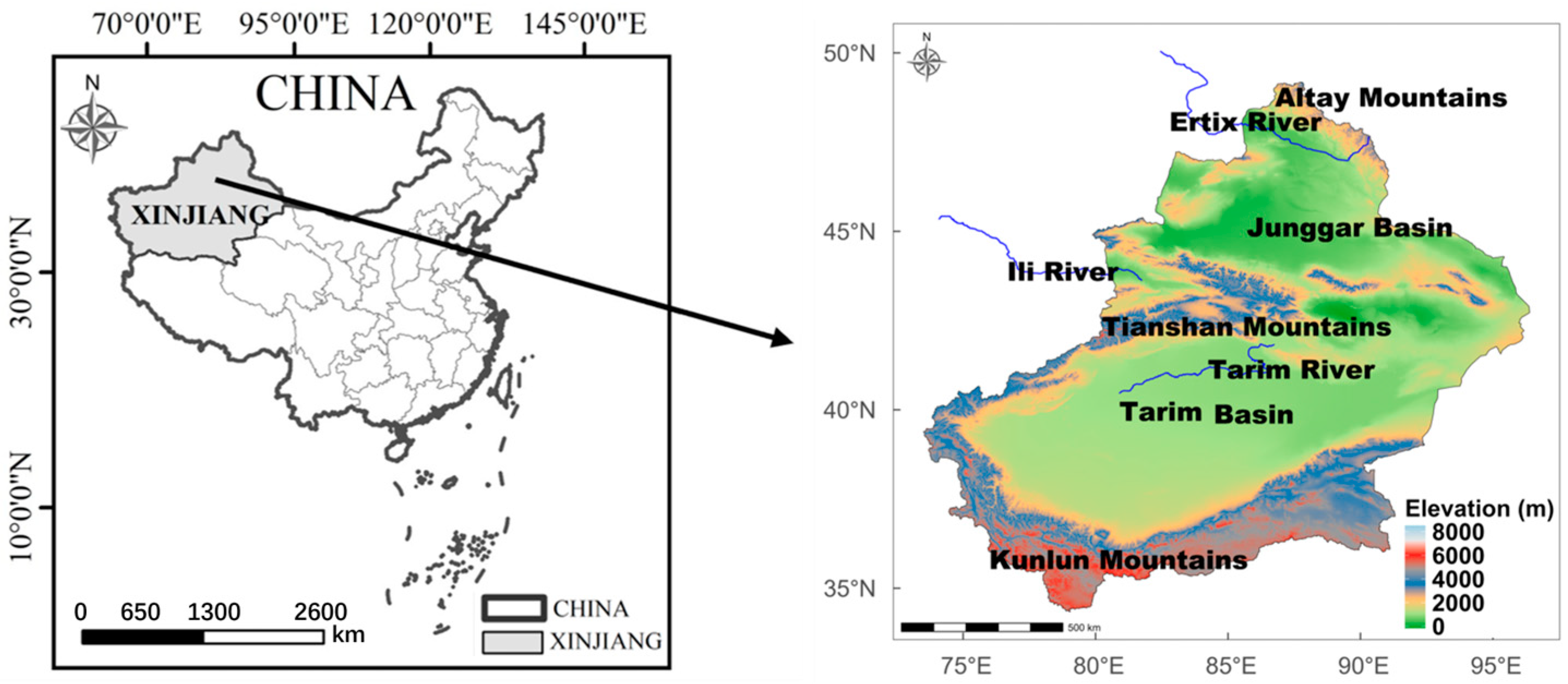
2.1. Study Area and Data

The Xinjiang region (73°40′ to 96°18′E, 34°25′ to 48°10′N) is in the northwestern part of China, situated far from any major oceans and distinguished by its unique geographical and geomorphic characteristics. Xinjiang exhibits a robust continental temperate arid climate, in contrast to the monsoonal climate in Eastern China. The climate in Xinjiang is primarily arid, with an average annual precipitation of approximately 100–200 mm. Precipitation is unevenly distributed, both spatially and temporally, with concentrations in mountainous regions and on the leeward sides of mountain ranges, whereas desert basins experience minimal precipitation. The topographical characteristics of Xinjiang are complicated. As shown in Figure 1, Xinjiang is typically characterized by “three mountains and two basins”. The Altai Mountains (peak elevation: 4374 m), Tianshan Mountains (7443 m), and Kunlun Mountains (7719 m) form the primary orographic barriers, enclosing the Junggar Basin and Tarim Basin. Major river systems include the transboundary Ertix, Ili, and Tarim, with the Tarim River spanning 1321 km along the northern rim of the Tarim Basin. Settlement networks are primarily concentrated on oases along river valleys and mountain foothills, notably Urumqi (elevation: 917 m), Kashgar (1290 m), and Yining (663 m), with sparse populations in desert areas.
The daily precipitation and minimum and maximum temperatures were obtained from the CN05.1 dataset [37], which contains high-resolution daily observational grid data over China for various meteorological parameters from more than 2400 national-level weather stations. These stations comprise basic, benchmark, and general stations. The Xinjiang region is clearly covered by multiple observation stations. Notable concentrations appear along mountain–basin transition zones. While station density is lower compared to Eastern China (due to geographic and population constraints), the interpolation methods including the thin-plate spline function (ANUSPLIN) and the Angular Distance Weighting method (ADW) with a resolution of 0.25° × 0.25° employed in CN05.1 are explicitly designed to account for such spatial heterogeneity by incorporating topographic covariates (elevation, slope, etc.) to improve prediction accuracy. This dataset has been widely used as observation data or a base dataset to investigate climate change patterns and for model simulation or comparison in Xinjiang [38,39,40], and it has also been used as observation data or a base dataset for model simulation and comparison [41,42,43]. The time range of the CN05.1 dataset in this study was 1961–2020.
The meteorological parameters, including daily precipitation (PRCP), maximum temperature (TMAX), and (TMIN) from CN05.1 dataset, were used to compute and analyze the climate extremes in Xinjiang. The overall trends of these three parameters are demonstrated in Figure 2, showing a clear “warming-wetting trend” in the past decades.

2.2. Methods

In this study, six extreme temperature indices and nine extreme precipitation indices (Table 1) were selected from the Expert Team on Climate Change Detection and Indices (ETCCDI) and calculated using the RClimDex software version 1.9 [44]. This study used the first three decades (1961–1990) as baseline data. The China Z index, hereby referred to as the Z index, describes the flood–drought severity [45,46], which has been applied in several studies, especially in China [47,48,49]. It divides flood–droughts into seven types (Table 2). The higher the Z index, the higher the flood severity; the lower the Z index, the higher the drought severity; normality is represented by values close to zero. The Z index was calculated as follows:
Z i = 6 C s C s 2 φ i + 1 1 3 6 C s + C s 6 ,
C s = i = 1 n x i x ¯ 3 n σ 3 ,
φ i = x i x ¯ σ ,
where i is the current month’s index, n is the number of months, C s is the skewness coefficient, and φ i ( i = 1 , , n ) are the normalized variables calculated using the climatic mean, x ¯ , and standard deviation, σ . To further analyze the overall periodicity of the Z index, we applied Morlet wavelet analysis, which is known for its multiresolution capabilities and ability to characterize the local features of signals in both the time and frequency domains. By decomposing the time-series into a time–frequency space, we identified the significant fluctuation patterns within the series, providing insight into the periodic change dynamics over time [50,51]. Additionally, we applied the Bayesian mutation test to detect significant shifts or mutations in periodicity, enhancing our understanding of abrupt changes and their corresponding time patterns [52,53].
To mitigate the potential impact of collinearity and distortion on the results induced by the number of variables, we used Random Forest (RF) and Best Subset Select (BSS) for variable selection, and applied the linear regression model (LM), Support vector regression (SVR), and RF as regression models to analyze the impact of climate extremes on the flood–drought severity in Xinjiang. The LM is a well-known traditional tool in the field of climate change and related extreme events [54,55,56], whereas SVR and RF, as relatively new machine learning models, were also generally used in recent studies [35,57,58,59].
BSS is a traditional statistical method for variable selection that evaluates all possible subsets of features to identify the best combination for model performance [60]. Despite its computational expense, BSS is effective for selecting a compact and predictive subset of variables.
RF is a powerful ensemble learning method used for both classification and regression tasks [61]. It operates by constructing multiple decision trees during training and outputs the average prediction of individual trees. In variable selection, RF evaluates the importance of features by measuring the decrease in Gini impurity or the Mean Decrease in Accuracy (MDA) for each feature. The higher the decrease, the more important the feature. The following equation shows the calculation of the Gini Index, a measure of node impurity used in decision trees to evaluate feature importance:
G = 1 Σ   p ( i ) ² ,
where G is a node and p ( i ) is the proportion of samples belonging to class i in the node. For each feature, X j , the RF algorithm calculates the reduction in the Gini Index after a split. If a feature, X j , is used for splitting a node, G , into two child nodes, G L and G R , the change in the Gini Index is computed as follows:
Δ G = G G L G G L + G R G G R ,
where G is the sample size of the original node and G L and G R are the sample sizes of the two child nodes. When training multiple decision trees, RF repeats the above process multiple times, calculating the average Gini Index reduction for each feature across all trees. Features that lead to a greater reduction in the Gini Index are considered more important for the model’s decision making. RF can also be used for regression analysis [62]. The output prediction is given as the average of all trees’ predictions. Given N decision trees and their predictions, f 1 x , f 2 x , , f N x , the RF prediction, F ( x ) , is calculated as follows:
F x = 1 N i = 1 N f i x  
To balance accuracy and computational efficiency, the ntree was set as 500 [63]. The parameter mtry was set to 1/3 of the total number of variables [64], and the parameter nodesize was set to 5 [65,66]. The RF models were calibrated via the package “randomForest” in R software version 4.4.1.
The LM is one of the most fundamental regression techniques, assuming a linear relationship between the independent variables (predictors) and the dependent variable (outcome). The model parameters are estimated by minimizing the sum of squared residuals (errors). The LM is widely used in various fields, including climate science and risk management, due to its simplicity and interpretability [67]. The basic idea of a linear regression model can be expressed as follows:
y = β 0 + β 1 x 1 + + β p x p + ε ,
where β 0 is the intercept, β 1 , …, β p are the coefficients of the independent variables, x 1 ,…, x p , and ε represents the error term.
The SVM theory proposed by Vapnik [68] was originally used for pattern recognition and supervised classification processes [69]. SVR refers to the implementation of SVM regression and estimation methods [70]. SVR aims to find a function that approximates the relationship between input features and target values by minimizing the following objective function:
m i n w , b , ξ , ξ * 1 2 w 2 + C i = 1 N ξ i + ξ i * ,
with the following constraints:
y i w , X i b ϵ + ξ i w , X i + b y i ϵ + ξ i * ξ i , ξ i * 0 , ,
where w is the weight vector, b is the bias term,   ε is the tolerance, ξ i , ξ i * are slack variables to account for errors, and C is the regularization parameter controlling the trade-off between the flatness of the function and tolerance to deviations. In SVR, the feature function, ϕ ( x ) , maps the input data into a higher-dimensional feature space. Kernel functions allow for computation in the feature space without explicitly calculating ϕ ( x ) . The kernel function,   K ( x ,   x ) , computes the dot product in the feature space as K ( x ,   x ) = ϕ ( x ) . ϕ ( x ) . By introducing the kernel function and Lagrange multipliers, α i ,   α i * ,   i = 1 , ,   N , the prediction function becomes as follows:
f ( x ) = i = 1 N α i α i * K X i , X + b
The kernel function of SVR was set as the radial basis function (RBF) as it is widely used for non-linear problems [71,72]. The kernel parameter gamma and the regularization parameter C were set as (1/number of features) and 1 based on previous studies [65,73]. The SVR models were calibrated via the package “e1071” in R software version 4.4.1.

3. Results

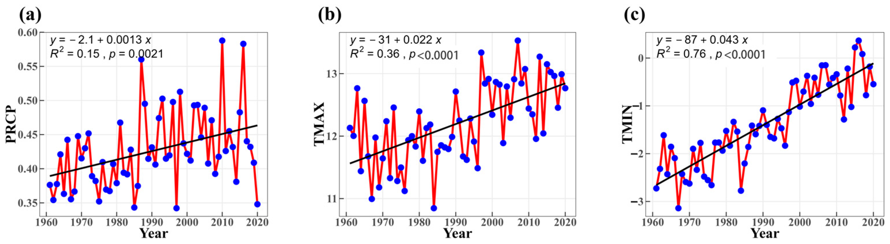
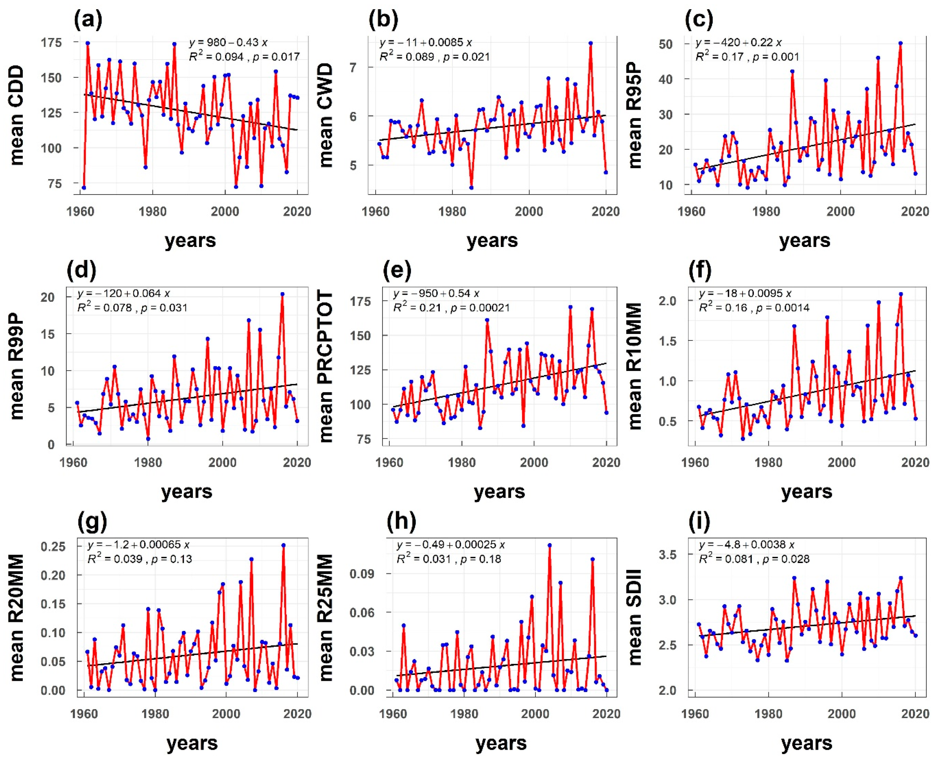
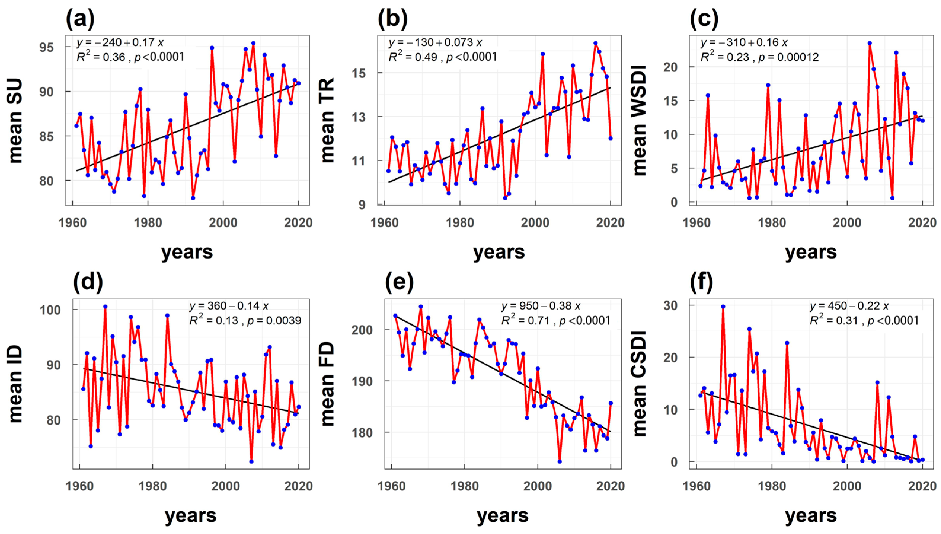
3.1. Climate Extreme Changes in Xinjiang

We first explored the linear trends in the annual extreme precipitation and temperature indices of the study area over six decades (Figure 3 and Figure 4). All extreme precipitation indices showed increasing trends, except for consecutive dry days (CDD, Figure 3a). The overall precipitation extremes increased significantly with p < 0.05 for most indices. In contrast, dry days decreased significantly by 0.43 days/year. Except for the wetting trends in the 1990s, there were some dramatic anomalies at certain points in the past few decades for both the frequency (Figure 3f–h) and intensity (Figure 3c–e). The extreme high or low values of these precipitation extremes, or the “extremes of extremes”, also increased significantly in recent decades.
The linear trends of six temperature extreme indices showed a “warming trend” in Xinjiang (Figure 4). All three indices for high-temperature extremes increased significantly (p < 0.01) at a rate of 0.17 days/year for summer days (SU), 0.073 days/year for tropical nights (TR), and 0.16 days/year for the warm spell duration indicator (WSDI) (Figure 4a–c). All three indices for low-temperature extremes decreased significantly (p < 0.01) at a rate of 0.14 days/year for ice days (ID), 0.38 days/year for frost days (FD), and 0.22 days/year for the cold spell duration indicator (CSDI) (Figure 4d–f). The hot temperature extremes showed clear positive changes since the 1990s, especially when TR completely showed a zero negative change during the past two decades. In contrast, the low-temperature extremes showed notable negative changes since the 1990s, especially when FD showed completely negative changes since 2000.

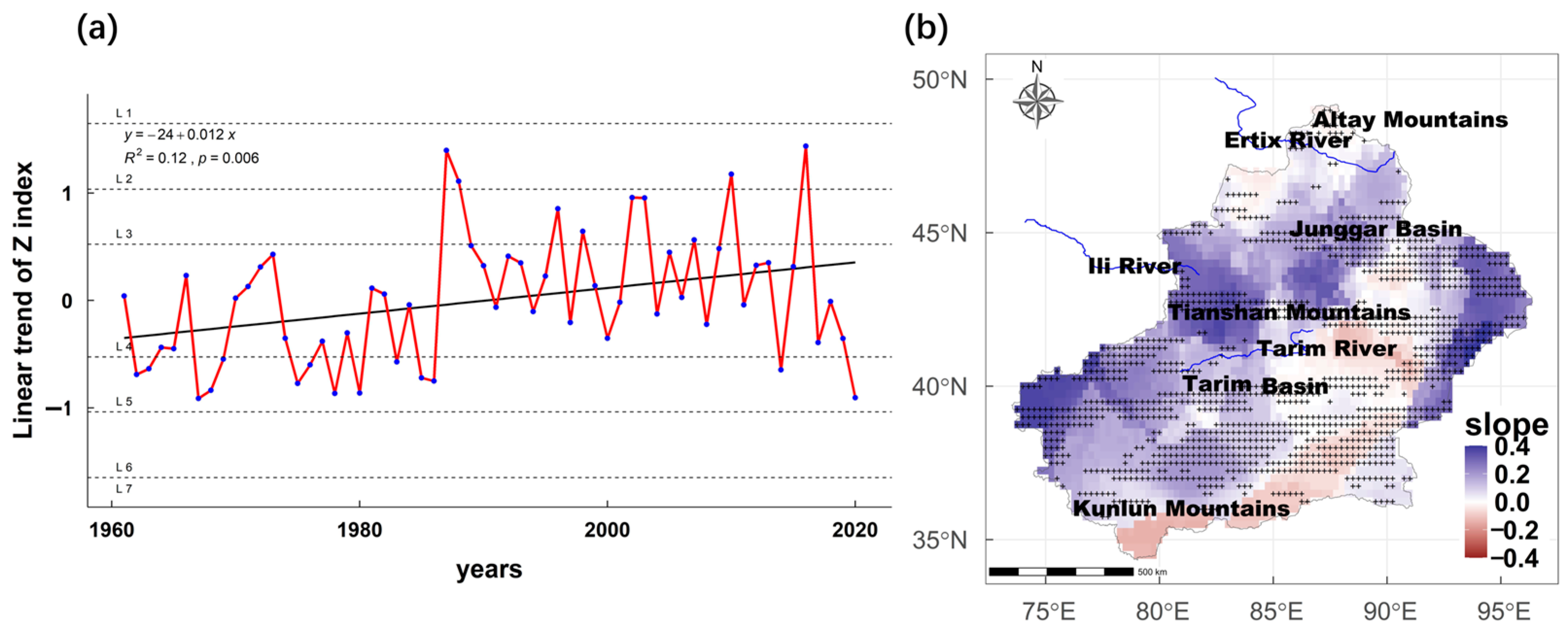
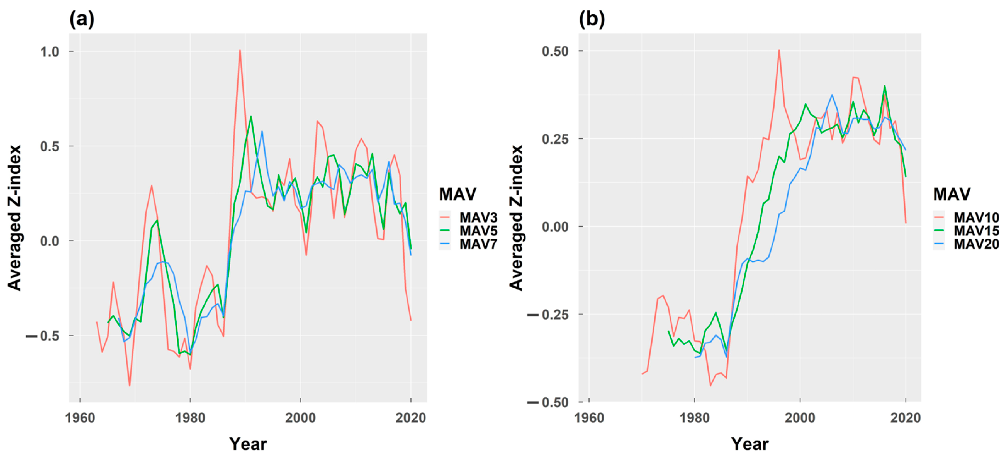
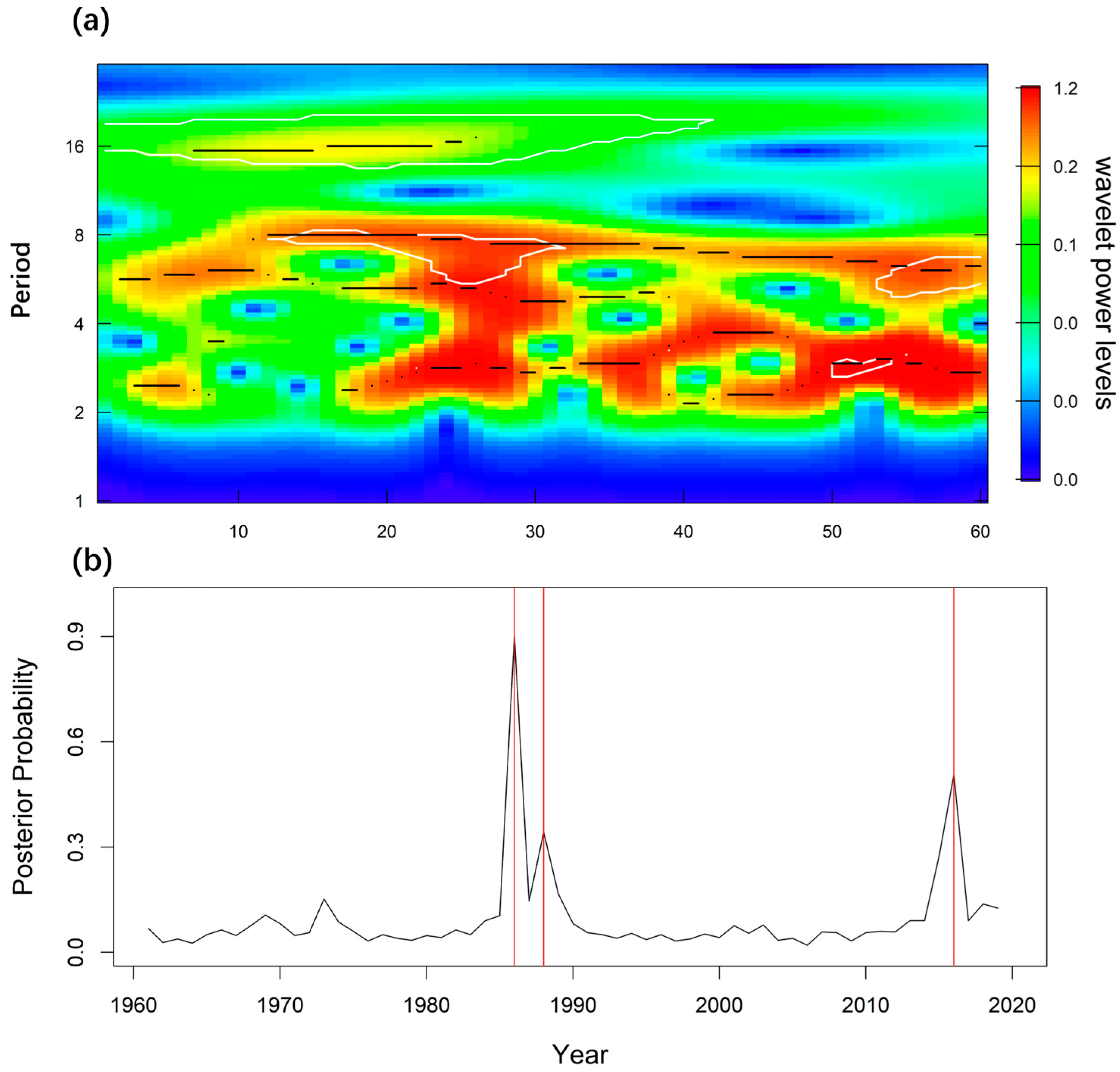
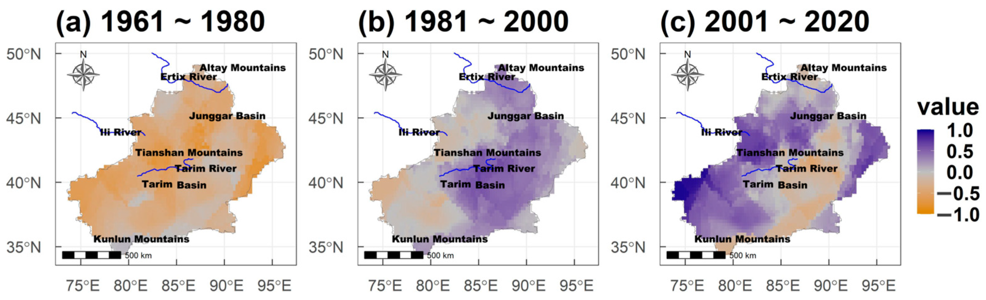
3.2. Flood–Drought Changes in Xinjiang

To better understand the flood–drought changes in Xinjiang, we first demonstrated the linear trends in the average annual Z index (Figure 5a). From 1961 to 2020, the Z index increased significantly (p < 0.01) in Xinjiang at a rate of 0.012/yr. The flood–drought types changed from L5 (light drought) to approximately L3 (light flood) or even L2 (serious flood). The flood–drought severity in Xinjiang changed from more droughts in the first three decades to more floods in the following decades.
To explore the spatial flood–drought changes in Xinjiang, the linear trend and corresponding significance level of the Z index were demonstrated (Figure 5b). Most parts of Western Xinjiang and part of Eastern Xinjiang, as well as the regions around the Ili River and Junggar basins, showed significant increases in the flood severity (0.1–0.4 per decade), while most parts of the Altay Mountains, Ertix River, Tarim River Basin, and Southern Xinjiang, as well as the Kunlun Mountains, showed increases in the drought severity, although these increases were not significant. The insignificance of the linear trend in the Ertix and Tarim River basins may be due to shifts in the flood and drought severities in certain areas. We also observed that Xinjiang’s overall spatial mean Z index over the six decades produced a twisted result (Figure A1). The range in the Z index of the entire Xinjiang region was compressed to −0.03 and 0.03 and completely lost the flood–drought change patterns in Xinjiang.
The changes in the flood–drought severity at different time scales in Xinjiang can also be observed through the moving averages of the Z index. Moving averages for smaller (Figure 6a) and larger time scales (Figure 6b) showed similar trends. Overall, the Z index in Xinjiang increased dramatically from approximately −0.5 to 1.0 the 1990s; it then slightly decreased to a negative value with a fluctuation in recent years, as in 2020.
We also explored the periodicity and mutations of the Z index (Figure 7). The results show that the annual Z index in Xinjiang from 1961 to 2020 had significant periods of 2.5 and 8 years (Figure 7a). We detected three significant mutations in 1986, 1988, and 2016.
To explore the spatial changes in the Z index in different time scales, we calculated the mean values for 10, 15, and 20 years (Figure 8, Figure A2 and Figure A3). Similar patterns were observed for both sets of results. Xinjiang was drought-dominant in the first two decades (Figure 8a and Figure A2a,b), and then shifted to mostly flood-dominant, except for part of Eastern Xinjiang in the following two to three decades (Figure 8b, Figure A2c–e and Figure A3c). During the previous two decades, a dramatic shift occurred in contrast to the former two decades (Figure 8b,c). The flood-dominant regions, including part of the Junggar Basin, Eastern Tianshan Mountains, and most parts of the Tarim River Basin from 1981 to 2000, reversed to drought-dominant from 2001 to 2020. The drought-dominant regions in the remaining areas, including most parts of Western Xinjiang from 1981 to 2000, reversed to flood-dominant from 2001 to 2020.
In addition to these shifts, the range of Xinjiang’s Z index has recently become significantly wider. As shown in the boxplots (Figure A4), the patterns were almost identical: the values and ranges of the Z index suddenly became significantly larger for the overall drought in the beginning (mostly before the 1980s) than during later periods, especially in the most recent decade from 2011 to 2020 (Figure A4a). More specifically, the box body of 2011–2020 ranged from below −0.5 to above 0.5, indicating that 50% of the mean Z index across whole Xinjiang was widely distributed. On the contrary, the mean Z index during 1961–1970 and 1971–1980 was mostly centered between −0.5 and 0, while that of 1991–2000 and 2001–2010 mostly centered between 0 and 0.5.
Table 3 lists the changes in the mean and standard deviations of climate extremes from 1961 to 2020 in Xinjiang. The mean (and standard deviation) R95P increased from 15.11 (4.41) during 1961–1980 to 24.91 (10.62) during 2001–2020, and that of R10MM increased from 0.61 (0.22) during 1961–1980 to 1.03 (0.48) during 2001–2020, whereas the mean of TR increased (with a nearly doubled standard deviation) from 10.86 (0.78) during 1961–1980 to 13.97 (1.49) during 2001–2020. In contrast, the standard deviation of WSDI increased slightly (with a more than doubled mean) from 5.4 (4.46) during 1961–1980 to 12.2 (6.34) during 2001–2020.

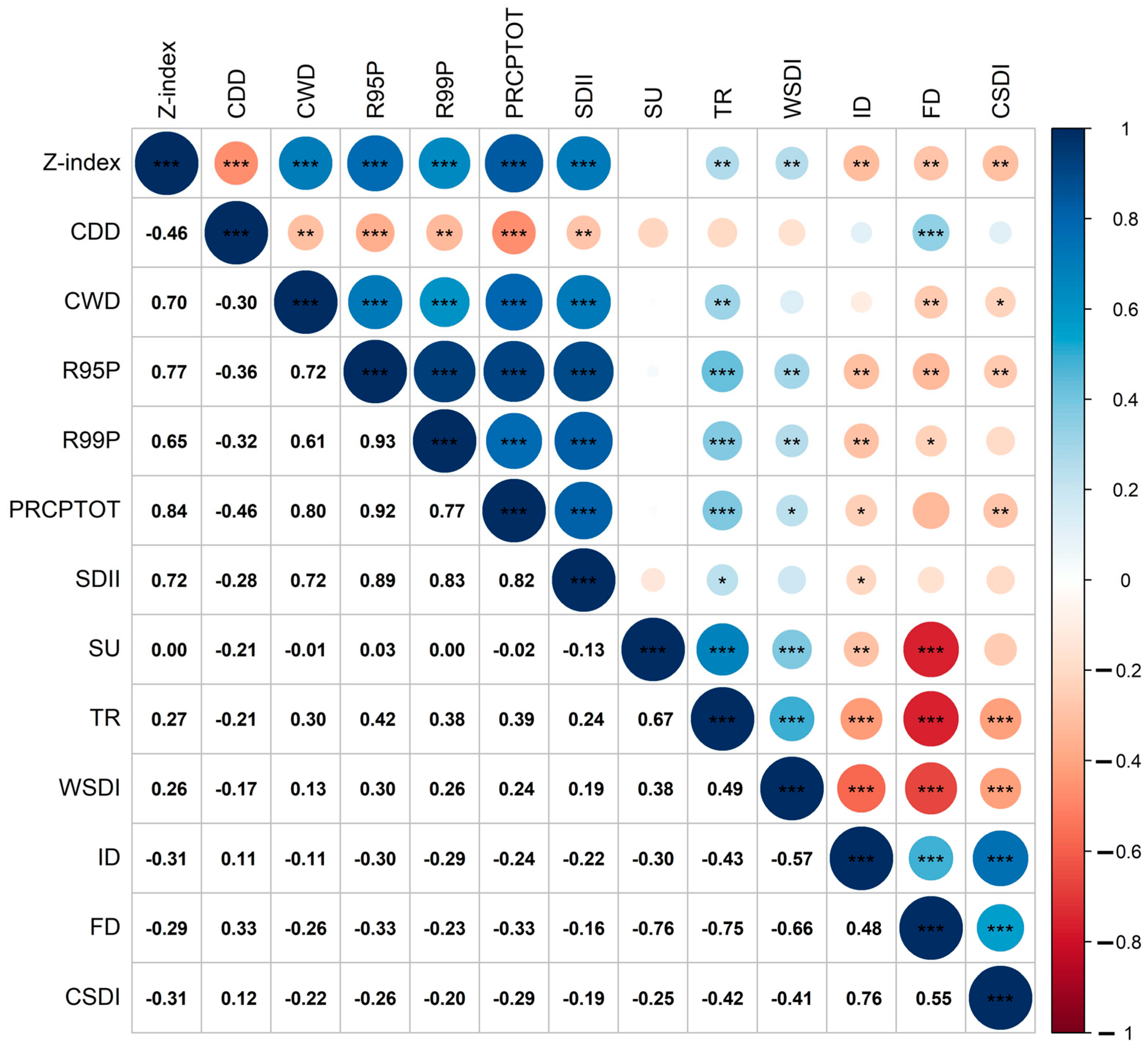
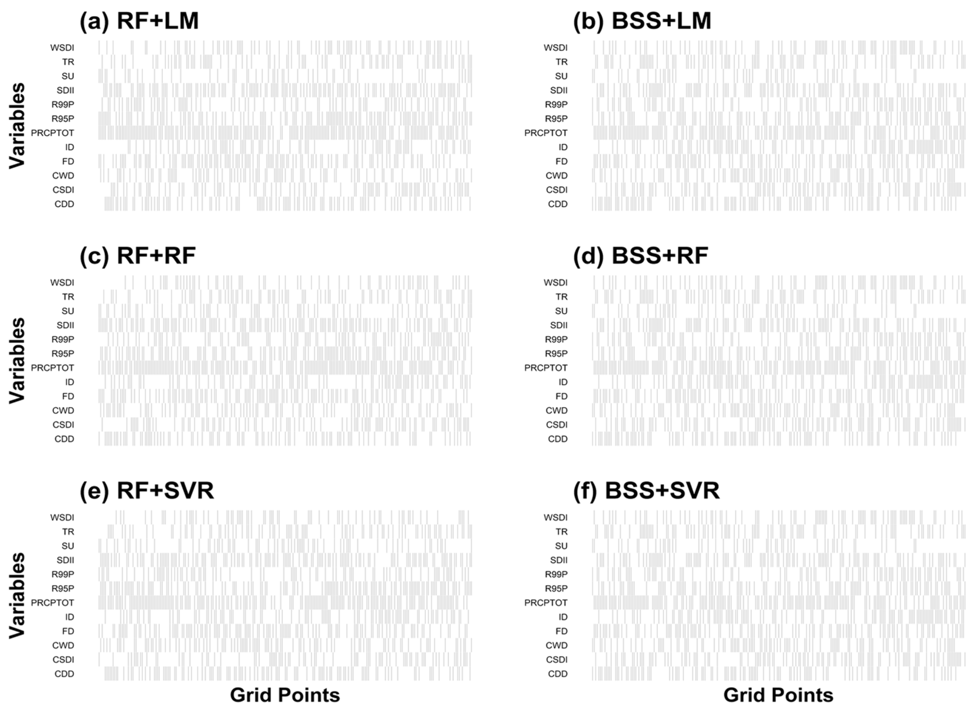
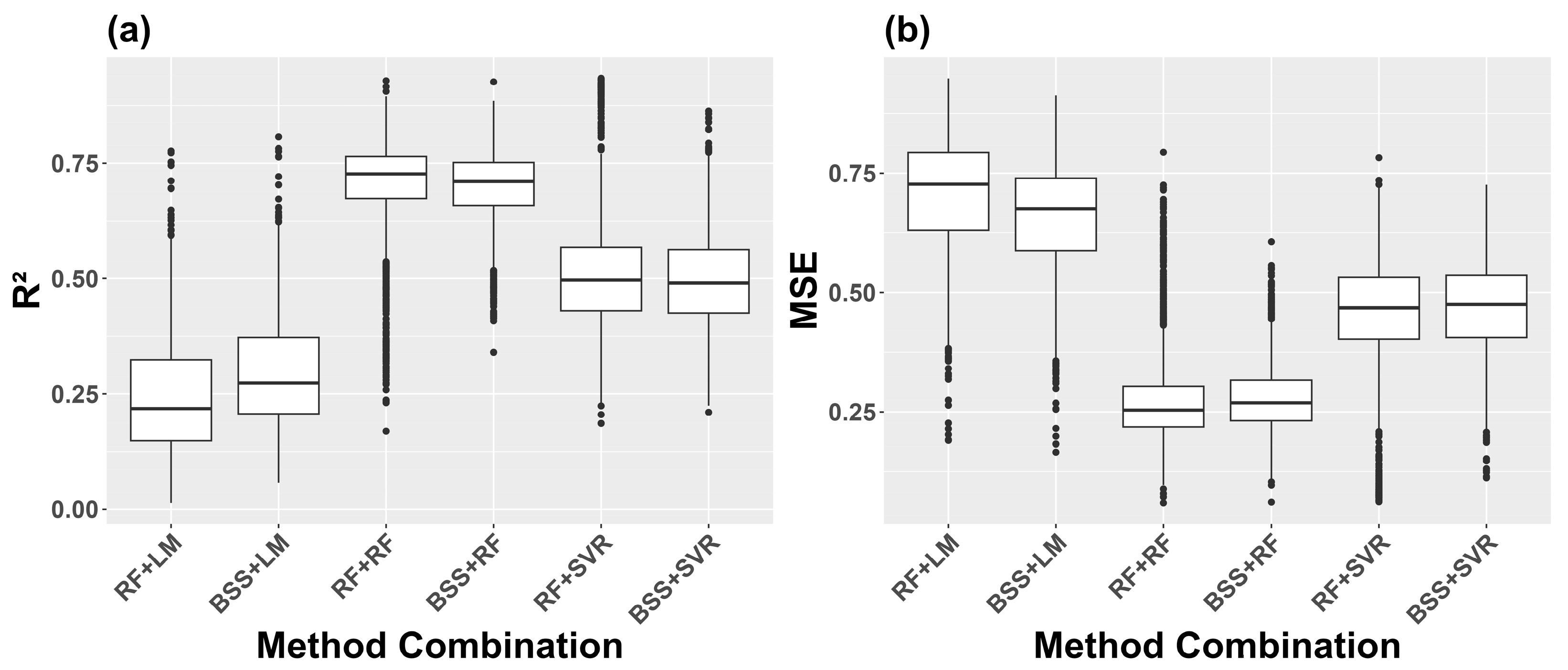
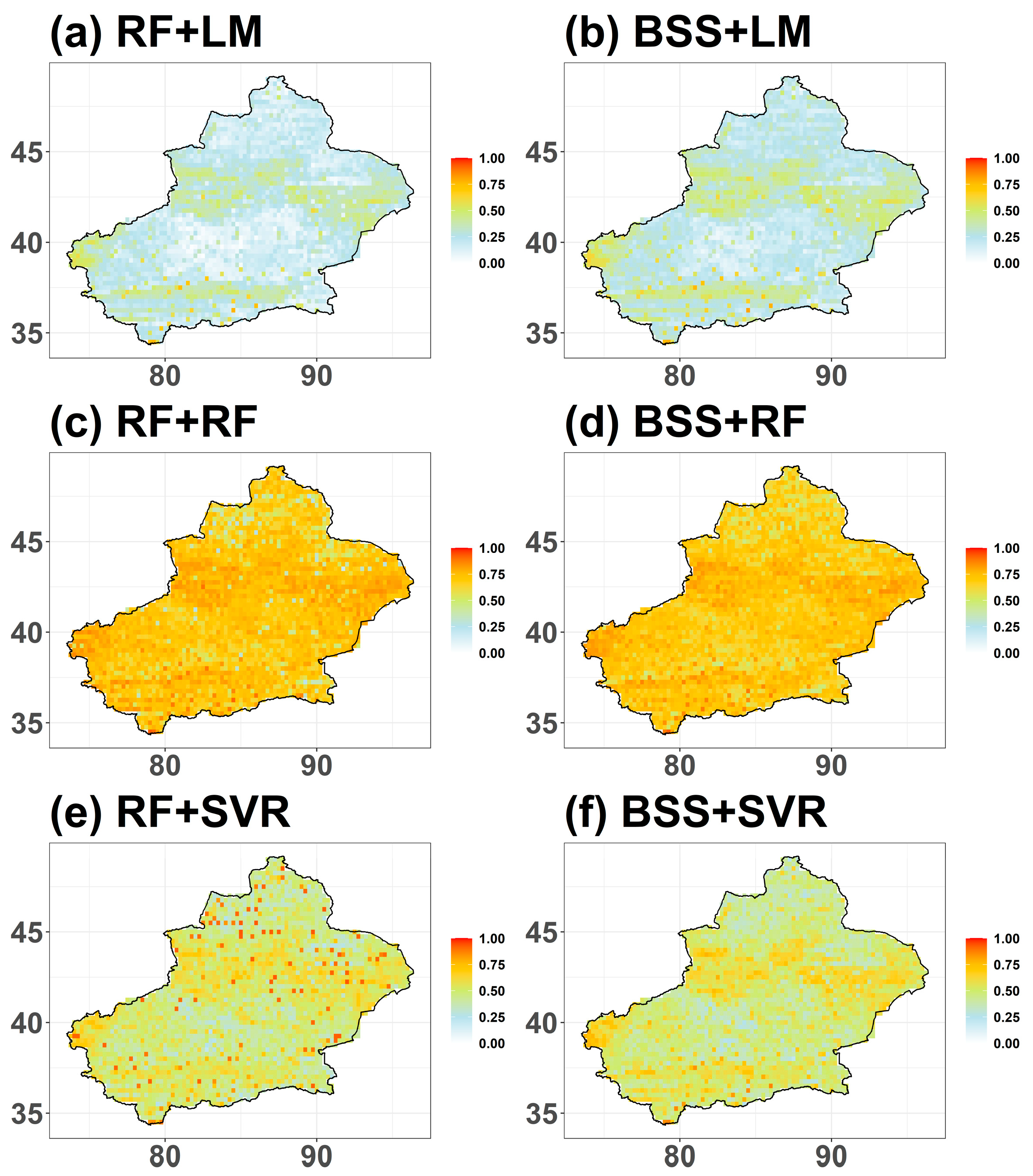
3.3. Impacts of Climate Extremes on Flood–Drought Severity

Considering the correlations between the flood–drought severity and climate extremes in Xinjiang, we calculated the overall and spatial correlation coefficients between the Z index. We selected extreme climate indices, including six temperature and precipitation extremes (Figure 9). We chose only 12 because the other three indices (R10MM, R20MM, and R25MM) were all zero for most years in some of the areas; thus, they were inappropriate for calculating the correlations.
Generally, the Z index showed a stronger positive correlation with the precipitation extremes, except for CDD (−0.46). Among them, the correlation with PRCPTOT was the highest at 0.84, followed by R95P (0.77), SDII (0.72), CWD (0.70), and R99P (0.65), whereas three of the temperature extremes showed a weaker negative correlation of the Z index with ID and CSDI, both at −0.31, and FD (−0.29). Two temperature extremes showed a weaker positive correlation with TR (0.27) and WSDI (0.26). SU did not show any clear correlation, likely due to a larger spatial non-stationarity.
Considering the potential spatial differences in the correlation between the Z index and these extreme indices, we also showed the spatial distribution of the correlation coefficients (Figure 10). Most results in the spatial distribution of the correlation coefficients between the Z index and these extreme indices were basically consistent with the overall correlation. Two of the temperature extremes and most precipitation extremes showed minor spatial differences (Figure 10d,f–l). However, three of the temperature extremes (SU, WSDI, and FD) exhibited significantly different and complex spatial patterns (Figure 10a,c,e). SU showed a positive correlation with the Z index, mostly around Eastern Xinjiang, the Junggar Basin, the western part of the Tianshan Mountains, and Western Xinjiang, including the Ili River, while showing a negative correlation in parts of Northern and Southern Xinjiang, the Tarim River Basin, and the eastern part of the Tianshan Mountains. The FD showed almost the opposite spatial pattern with SU; there was mostly a negative correlation around the small part of Eastern Xinjiang, the Junggar Basin, the western part of the Tianshan Mountains, and Western Xinjiang, including the Ili River. There was a positive correlation in the small parts of Northern and Southern Xinjiang, the Tarim River Basin, and the eastern part of the Tianshan Mountains. The Z index and TR correlation did not show any clear spatial patterns.
Based on these correlations, we further analyzed the impacts of these climate extremes on the Z index. By applying variable selection techniques (RF and BSS) and regression models (LM, RF, and SVR), we generated six method combinations: “RF+LM”, “BSS+LM”, “RF+RF”, “BSS+RF”, “RF+SVR”, and “BSS+SVR”. Based on the spatiotemporal data in this study, we applied these six method combinations for each grid across the entire study area.
Figure 11 and Table 4 present the results of the pointwise variable selection and the most frequently selected variable for the six method combinations. In Figure 11, the colored variables in each column represent that the variables were selected on the current location under the corresponding method. The selected variables were different across the grid points in Xinjiang; all six methods showed spatial heterogeneity in the selected variables. Moreover, there was an impact within most of the extreme climate indices on the flood–drought severity across >30% of Xinjiang (Table 4). However, only four to seven indices were selected with a frequency >40% across the entire study area. Only PRCPTOT, R95P, and SDII were selected in >50% of the areas. Despite the spatial heterogeneity of the impacts of these climate extremes on the flood–drought severity, there are still certain key indices that play the most important roles in most areas of Xinjiang.
Figure 11, Figure 12 and Figure 13 and Table 5 present a summary and the spatial distributions of the R2 and MSE of the six method combinations. The overall performance of the method combination of RF+RF was the best. The R2 of this method across the entire study area was approximately 0.75 (Figure 12a), with a mean value of 0.71 (Table 5). The BSS+RF method, with an R2 of 0.70, also showed better performance. Based on the spatial distribution, the R2 of RF+RF and BSS+RF in most areas was higher than the other method combinations (Figure 13). The MSE of these two methods showed similar advantages compared with the other methods, with a mean MSE of 0.27 and 0.28, respectively (Table 5). Their MSE values across the entire study area were also approximately 0.25 (Figure 12b and Figure 14c,d). However, the variable selection results of RF+RF and BSS+RF showed certain differences in all three cases (Frequency > 30%, Frequency > 40%, and Frequency > 50%). Other method combinations, including LM and SVR, showed lower prediction abilities. The performances of LM-based models were generally lower with a mean R2 < 0.3 (Table 5), and the fluctuations in their R2 and MSE values were larger than the other method combinations (Figure 12). Notably, RF+SVR showed extremely high values in R2 and extremely low values in MSE (Figure 12). However, the spatial distribution of these extreme high values did not show any spatial pattern (Figure 13e and Figure 14e).

4. Discussion

4.1. Fluctuation in Climate Extremes and the Spatiotemporal Variabilities of Flood–Drought Severity

Under the effects of global warming and climate change in arid Central Asia (CA), there have been significant changes and climate extremes in Xinjiang. Previous studies have shown that the “warming-wetting trend” in Xinjiang has been notable since 1961 [19,74]. Although increasing precipitation during recent decades may have partially eased dryness, the true nature of arid and semi-arid Xinjiang has not changed [19,21].
In this study, we also showed that, despite the so-called “warming-wetting trend” certain uncertainties still occurred for the temperature and precipitation extremes, especially during the most recent two to three decades. Figure 3, Figure 4 and Figure 5 indicate that the frequency and intensity of precipitation extremes increased in Xinjiang for several decades, or a “wetting trend” had occurred; this may have resulted in higher flood risk in specific areas of Xinjiang. However, along with the overall wetting trend, the frequency and intensity of extreme precipitation also showed a notably increasing fluctuation; the ranges of the mean values for some indices doubled in recent decades compared to previous decades. For example, the values of R95P (Figure 3c) were <20 mm for almost the entire 1961–1990 period, but they suddenly increased to 40 mm, especially near 2020. Most of the other seven indices showed a similar range increase; these indices decreased dramatically, except for the sudden increase in the CDD near 2020. These increases in uncertainty and fluctuation in the precipitation extremes may result in sudden floods in Xinjiang. On the other hand, hot temperature extremes showed clear positive changes after the 1980s. TR increased with stronger uncertainty (Table 3).
In contrast, the low-temperature extremes also showed a notable decrease since the 1990s. More specifically, The FD showed significant decrease during the last two decades; the three low-temperature extremes have decreased steadily, especially the mean of the CSDI, which decreased dramatically from 12.12 to 2.86 in Table 3. All of these increases in uncertainty and fluctuation in the CDD and the three hot temperature extremes may result in more frequent and severe droughts in Xinjiang, and the decrease in all of the low-temperature extremes may increase the flood risk, associated with the increase in the precipitation extremes mentioned above.
Along with these increases in climate extremes, flood and drought levels and potential risks have also increased significantly. Previous studies indicate that drought in Xinjiang was spatially and seasonally uneven, mostly showing a decreasing trend in Northern Xinjiang and an increasing trend in Southern Xinjiang, with slight decreases in autumn and winter, but increases in spring and summer [75]. Floods in Xinjiang have also increased since the mid-1980s, occurring near the Ili River and part of South Xinjiang from March to October. The frequency and damage of precipitation-induced floods have increased 3.8–5.6-fold [76]. Generally, drought in Xinjiang decreased before the 1990s, then showed a reverse trend after 1997 [77]. Since 1997, over 70% of Xinjiang has experienced intensified aridification, characterized by significant warming, enhanced potential evapotranspiration, and a slight reduction in precipitation, leading to increased drought frequency. A distinct climatic regime shift from warm-wet to warm-dry conditions emerged in the late 1990s, marking a pronounced wet-to-dry transition [18]. Mechanistic studies highlight the Atlantic Multi-decadal Oscillation (AMO) as a key driver, exhibiting a significant negative correlation with the Standardized Precipitation Evapotranspiration Index (SPEI) in Xinjiang. Positive (negative) AMO phases correspond to drier (wetter) periods, particularly post-1997. During AMO-positive phases, the intensified Indian summer monsoon enhances precipitation over India while suppressing summer rainfall in Xinjiang [78,79]. Additionally, regional drivers such as decrease in relative humidity and increase in wind speed could contribute to the redrying trend in Xinjiang [21].
In this study, the annual and spatial trends in flood–drought severity were similar to those of previous studies. Despite the general increasing trend, the Z index decreased slightly during the last two to three decades, especially in the last few years close to 2020, when there was a sudden drop in the Z index (Figure 5). The flood–drought type constantly reversed, finally almost reaching L6 (serious drought) in 2020. Except for the results of the wavelet analysis showing 2.5- and 8-year periods in the flood–drought severity, the mutation in 2016 also indicates that the overall wetting trend of Xinjiang during the last few decades since 1980s may have also reversed back to a drying trend. The overall flood–drought level of Xinjiang showed a pattern of “drought–flood–drought.” However, we only focused on the overall temporal changes; therefore, we may have lost important regional information at different time scales. In Figure A1, there was no clear spatial difference or any pattern in the mean annual Z index over the entire 60 years, which conflicted with the results shown in Figure A2, Figure A3 and Figure 8. As we mentioned earlier in Section 3.2, The range in the Z index of the entire Xinjiang region was compressed to −0.03 and 0.03. In addition to overall periodical changes shown in Figure 7a, the reason for this misleading result might be the changing patterns of spatial heterogeneity which we will discuss further in the next comment. More specifically, spatial shifts between low and high values in regional Z index were clear in Figure A3, the regional values between a and c, as well as b and d were mostly opposite, which leads these pairs of values cancel each other out and resulted in overall near-zero values in Z index.
We have shown an overall significant increase in the mean of the Z index, along with a slight increase in the standard deviation from −0.37 (0.43) during 1961–1980 to 0.22 (0.61) during 2001–2020 (Figure A4c). However, no significant difference existed between 1981 and 2000, and between 2001 and 2020. Therefore, we must examine different spatiotemporal scales to examine spatial heterogeneity in the flood–drought severity. The spatial distribution of the Z index showed a clear transition from overall drought dominance in the 1960s and 1970s to overall flood dominance in the 2000s (Figure A2a,e and Figure A3a,c). However, notable spatial heterogeneity occurred in other periods. Regional differences have become larger, especially near 2020 (Figure 8c, Figure A2f and Figure A3d), which may result in spatial differences in the linear trends (Figure 5b), where insignificant drought trends have occurred near the Altay Mountains, Ertix River, part of the Tarim River Basin, and the Kunlun Mountains, in contrast with the most significant increase in flood levels across the rest of Xinjiang. These results indicate that exploring potential flood–drought risks in Xinjiang and their causes could be more complicated.

4.2. Flood–Drought Shift in Xinjiang

Except for the annual change and fluctuations in the flood–drought severity at different time scales, there was also a dramatic spatial shift. The spatial distribution of the flood–drought level during 1981–2000 shifted to a reversed distribution from 2001 to 2020 (Figure 8b,c). The areas characterized by the drought dominant to flood dominant shift were mostly focused on parts of East Xinjiang and most of West Xinjiang while the reversed shifts were distributed in North Xinjiang, including the Altay Mountains and Ertix River, eastern part of the Tianshan Mountains and Tarim River Basin, and the Kunlun Mountains. The areas with a flood–drought shift mostly occurred in the Junggar Basin, Tianshan Mountains, Tarim River Basin, and East and West Xinjiang, including the Ili River. In contrast, the Z index’s means, medians, and standard deviations in these two periods showed no significant changes except for a slight increase (Figure A4c and Table 3). These inconsistencies in the overall and regional changes may induce unexpected floods or drought events. For example, floods occurred in June 2013 in Xinjiang, resulting in more than 6000 houses and approximately 12,000 hectares of cropland damage after suffering from unusual snowstorms (https://floodlist.com/asia/china-june-2013, accessed on 11 November 2023). Devastating floods induced by extreme rainfall in Hami City of Xinjiang in July 2018 caused 20 deaths and the evacuation of more than 5000 people [80]. The abrupt flood–drought changes resulted in the largest reservoir area in China, as analyzed by Cui et al. [81]. Notably, a part of Eastern Xinjiang, the location of Hami, showed a consistent increase in flood–drought severity (Figure 5b); most of this area showed flood–drought shift in Figure 8. This “used to be drought” area may have transferred to an area with higher flood risks near 2020. Therefore, the floods in July 2018 could be captured by this study.
However, the causes of the flood–drought shifts require further investigation. As a typical arid and semi-arid region of CA, Xinjiang is extremely sensitive to climate change. Global warming increases atmospheric water vapor and evaporation, influencing the precipitation and water cycle [82]. Precipitation can be stored in soil within a short period, but a drought may occur if there is a long heatwave or the lack of a water supply [83]. Followed by a drought event, once extreme precipitation exceeds the capacity of water storage of soil, the risk of natural hazards, such as landslides [84] or floods [85], increases, especially in the mountainous areas of Xinjiang. Therefore, analyzing the relationships between flood–drought severity and climate extremes is necessary. In this study, we showed the spatial distributions of the correlations between the Z index and the SU, WSDI, and FD, with clear spatial non-stationarity (Figure 10a,c,e). Such spatial patterns may result in seemingly weaker correlations, as shown in Figure 9. Moreover, as demonstrated in Figure 4a,c,e, the highest and nearly the highest values of the SU and WSDI occurred from 2000 to 2020, while the lowest points of the FD were concentrated in these two decades. These extremes may have influenced the dramatic shift in these two decades more than in the previous. The correlations between the Z index and both SU and WSDI were positive in most parts of the Junggar Basin, Western Xinjiang, and a small part of Eastern Xinjiang; this was negative in a small part of the Junggar Basin and most parts of the Eastern Tianshan Mountains, as well as the Tarim River Basin (Figure 10a,c). In Figure 10e, the Z index and FD correlations were almost the opposite of the other two climate indices above. These correlations were consistent with the spatial distribution of the flood–drought level shifts in Figure 8c. The spatiotemporal characteristics of climate extremes and their correlation with the Z index are most likely to influence flood–drought severity in Xinjiang.

4.3. Potential Driving Factors of the Changes in Flood–Drought Severity

The correlation between extreme climate indices and the Z index in Xinjiang, combined with the results of the regression models and variable selection methods, allows us to assess the relative effectiveness of different approaches in capturing the drivers of flood–drought variability. In this study, the six method combinations were RF+LM, BSS+LM, RF+RF, BSS+RF, RF+SVR, and BSS+SVR. The results clearly indicate the superior performance of RF+RF (Random Forest for both variable selection and regression) and BSS+RF (Best Subset Selection for variable selection and Random Forest for regression), with RF+RF emerging as the most effective method in managing variable interactions and handling the complexities of extreme climate influences on flood–drought dynamics.
The RF+RF method showed the highest mean R2 value (0.71) and the lowest mean MSE (0.274), indicating that it provided the most accurate fit across the study area. This method effectively manages non-linear relationships and multicollinearity between the selected variables, a critical advantage in this context where extreme climate indices, such as PRCPTOT, R95P, and SDII, strongly influence flood–drought severity in most areas of Xinjiang. In contrast, other methods, particularly LM-based approaches (e.g., RF+LM and BSS+LM), exhibited significantly lower performance, with mean R2 values below 0.3 and larger MSE values. The poor performance of linear models in this case demonstrates their inability to capture the complex and non-linear interactions among the climate indices that drive flood–drought variability in Xinjiang.
BSS+RF also performed well, with a mean R2 of 0.70 and a mean MSE of 0.28. Although it is close in accuracy to RF+RF, it differs in its variable selection results. This difference reflects the methods’ ability to handle spatial heterogeneity and variable selection frequency. While both methods basically select similarly, RF+RF shows greater robustness in managing multicollinearity between variables. BSS+RF selected more variables in the following two cases: WSDI in the low (>30%) CSDI and ID in the medium (>40%) frequency. RF+RF selected R95P in the high (>50%) frequency while BSS+RF did not. These indices showed relatively higher correlation with the other indices with similar characteristics. Correlations between WSDI and FD, CSDI and ID, and R95P and PRCPTOT were −0.66, 0.76, and 0.92, respectively (Figure 9). However, R95P, as an intensity index of precipitation extremes, is unignorable in the field of risk management. The most extreme values in precipitation may play a key role in causing sudden flood, especially in an arid region such as Xinjiang, e.g., the floods in June 2013 (https://floodlist.com/asia/china-june-2013, accessed on 11 November 2023) and July 2018 [80]. The ability of the RF+RF method combination to handle correlated variables and maintain the key indices makes it more effective than BSS+RF in certain regions. Furthermore, it does not rely on the traditional assumptions of variable independence among these climate extremes.
The findings from this study align with previous research on flood risk and climate extremes. For instance, Wang et al. [86] and Coelho et al. [87] both highlight the increasing importance of precipitation extremes in driving flood risks. In the study of the Louisiana flood, complex spatial patterns of extreme precipitation were found to contribute to local flood risk [86], similar to the spatial variability observed in the correlation between the Z index and indices such as PRCPTOT, R95P, and SDII in Xinjiang in this study. Moreover, Coelho, Ferreira, Johnston, Kinter III, Dollan and Maggioni [87] demonstrated the growing importance of accurately predicting extreme precipitation for flood engineering design. Furthermore, Swain et al. [88] emphasized the compounded effects of climate change and extreme weather events on flood risk in the U.S., a pattern also observed in Xinjiang, where climate extremes, such as CDD, FD, PRCPTOT, R95P, and SDII, exert substantial influence on flood–drought dynamics. These global studies reinforce the utility of advanced non-linear methods such as RF+RF in managing complex, multi-dimensional interactions driving flood–drought variability.
Spatial heterogeneity is another critical aspect highlighted by the variable selection results. In Figure 9, we have demonstrated the regional differences in the correlations between Z index and climate extremes. Considering the potential effects of these extremes on the spatial heterogeneity of flood–drought severity, we have applied six method combinations grid by grid. Both RF+RF and BSS+RF demonstrate the ability to capture localized variations in the importance of climate extremes. For instance, Table 4 indicates that although PRCPTOT, R95P, and SDII were selected frequently across most part of the study area under the RF+RF method, other indices such as CDD and FD also exhibited spatial variability in their importance in more than 40% of the area. Notably, FD showed clear regional characteristics in the correlation with Z index in Figure 9. Negative correlations were mostly focused on the small part of Eastern Xinjiang, the Junggar Basin, the western part of the Tianshan Mountains, and Western Xinjiang, including the Ili River, while positive correlations were in the small parts of Northern and Southern Xinjiang, the Tarim River Basin, and the eastern part of the Tianshan Mountains. The reason for this might be related to the complex regional climate in Xinjiang, where the northern and southern parts show almost the opposite responses for cold weather. These regional characteristics in the correlation between Z index and FD are similar with the spatial distribution of the linear trend of Z index and the patterns of spatial shift between two 20-years around 2000. These findings indicate that the overall decrease in cold extreme in Xinjiang might be able to partly explain spatial heterogeneity of flood–drought severity.
This study also highlights the spatiotemporal characteristics of climate extremes and their linkage to flood–drought shifts in Xinjiang. While the findings align with the broader “warming-wetting trend” observed in CA and Northwest China, the causal mechanisms driving regional spatial heterogeneity—such as intensified precipitation extremes around Tianshan Mountain versus aridification in Southern Xinjiang—require deeper exploration. Beyond local temperature and precipitation extremes, these shifts likely arise from complex interactions between large-scale teleconnection patterns and regional environmental dynamics: the Atlantic Multi-decadal Oscillation (AMO) phases correlate with dry-wet cycles in Xinjiang, where a positive AMO strengthens the Indian monsoon but suppresses Xinjiang’s summer rainfall via shifts in the South Asian high and westerly jet, while ENSO influences drought conditions in Northern Xinjiang with a 12-month lag, linking La Niña (El Niño) to dry (wet) anomalies [18,78,79]. Regional factors, including Xinjiang’s mountain-basin topography, amplify hydro-meteorological risks [82], as declining wind speeds and rising heatwaves exacerbate drying [21,89] while broader CA climate dynamics and oscillations like the North Atlantic Oscillation (NAO) and Interdecadal Pacific Oscillation (IPO) further contribute to spatiotemporal variability [21,90]. These findings underscore the need to integrate multi-scale drivers—from teleconnection patterns to localized feedbacks—to unravel the mechanisms behind Xinjiang’s evolving flood–drought transitions.
The ability to account for these spatial differences is essential for developing localized flood–drought prediction and management strategies, further underscoring the superiority of non-linear methods such as RF+RF and BSS+RF over more traditional linear models. In summary, the BSS+RF method, with its ability to manage multicollinearity and complex variable interactions, emerges as the most effective tool for analyzing flood–drought dynamics in Xinjiang. This method outperforms others in terms of both the R2 and MSE, offering greater predictive accuracy and robustness in managing spatial heterogeneity. The results of this study, when compared with global research, reinforce the need for sophisticated non-linear modeling techniques to better understand and predict the impacts of climate extremes on flood–drought severity and the related disaster risk management.

4.4. Uncertainties and Limitations

This study explored the changes and dramatic shifts in climate extremes and flood–drought severity and their spatiotemporal correlations in Xinjiang over the last six decades (1961–2020). However, certain uncertainties and problems remain. Utilizing interpolated grid data CN05.1 may introduce uncertainties due to the sparsity of meteorological stations in Xinjiang. The interpolated CN05.1 grid data with resolution of 0.25° × 0.25° may increase the bias regarding the results of some areas, such as the Tarim Basin and mountainous areas. In future studies, datasets with higher resolution and lower bias are needed.
There may also be new perspectives through further analysis of the seasonal or monthly changes in flood–drought severity. The relationships between flood–drought severity and other climate extremes also require careful consideration due to the collinearity between these climate extremes. Larger areas with different data sources and scale indices may also increase the uncertainty of our results. We analyzed the correlations between the flood–drought index and climate extremes, followed by the potential impacts of these indices on flood–drought severity. However, apart from the regional characteristics of temperature and precipitation changes, there could be other factors and overall changes in larger areas, such as the Northwest part of China or entire CA that include Xinjiang, which may also need to be considered. CA has exhibited significant warming and wetting trends in recent decades [91,92]. Wind speed and relative humidity can also contribute to the wetting–drying trend in Northwest China [21]; droughts combined with heat waves have increased in CA along with an increase in the global temperature [93]. Other larger-scale events, such as ENSO, North Atlantic Oscillation (NAO), and Interdecadal Pacific Oscillation (IPO), could also influence the flood–drought changes in Xinjiang or the entire CA [21,48,90].

5. Conclusions

This study explored the annual changes and fluctuations in climate extremes and certain spatial shifts in flood–drought severity, as well as their spatiotemporal correlations. The results provide scientific guidance for future disaster management and adaptation policies in arid and semi-arid regions. The main conclusions are as follows.
(1) Overall, Xinjiang’s “warming–wetting trend” in recent decades is already recognized as a fact, but the growing uncertainties are also unignorable. Precipitation, including CWD, R95P, R99P, R10M, and PRCPTOT, and temperature extremes, including TR and WSDI, have shown larger fluctuations than the former in the past two decades (2001–2020).
(2) The flood severity in Xinjiang increased for the first few decades, almost reached L1 (extreme flood), then decreased slightly during the recent two to three decades along with constant fluctuations, and almost reached L6 (serious drought) by 2020, which is consistent with the result of the mutation that occurred in 2016. The overall flood–drought level of Xinjiang changed from drought- to flood-dominant for a longer period but reversed to drought-dominant again near 2020. The results of the wavelet analysis showed a 2.5- and 8-year cycle of the Z index. The linear trends in the Z index showed clear spatial heterogeneity, with variations from −0.1 to 0.4 in distinct parts of Xinjiang.
(3) Flood–drought severity showed a dramatic spatial shift: certain areas of Xinjiang from 1981 to 2000 shifted to a spatially reversed distribution from 2001 to 2020, despite insignificant changes in the overall means, medians, and standard deviations in the Z index in these periods.
(4) The correlations between the flood–drought patterns and climate extremes are complex. The Z index showed the highest overall correlation with PRCPTOT (0.84), followed by R95P (0.77), SDII (0.72), CWD (0.70), and R99P (0.65). Despite three of the temperature extremes, including SU, FD, and WSDI, showing weaker correlations with the Z index, the spatial heterogeneity in the correlations and the most extreme values of these three indices all occurred in the last two decades (2001–2020), which may have influenced the dramatic shift in the flood–drought severity.
(5) Compared to other method combinations, RF+RF and BSS+RF performed the best, with high accuracy and robustness (mean R2 of 0.71 and 0.70, respectively, and mean MSE of 0.27 and 0.28, respectively) in capturing the impacts of climate extremes on flood–drought severity. RF+RF showed a better ability in managing collinearity. The impacts of CDD, FD, PRCPTOT, R95P, and SDII on flood–drought severity were most significant at the >40% selected frequency across the entire study area.

Author Contributions

Conceptualization, Y.Y.; Data curation, J.B., X.H., T.L. and J.J.; Formal analysis, S.N.; Funding acquisition, A.B.; Investigation, S.N.; Methodology, S.N., X.H. and T.L.; Project administration, A.B.; Resources, J.B., R.H., T.Y., T.W. and G.L.; Software, S.N. and G.L.; Supervision, A.B., Y.Y., R.H. and P.T.; Validation, J.B., T.Y., T.W. and J.J.; Visualization, S.N.; Writing—original draft, S.N.; Writing—review and editing, A.B., Y.Y., R.H. and P.T. All authors have read and agreed to the published version of the manuscript.

Funding

This study was jointly supported by the Key R&D Program of Xinjiang Uygur Autonomous Region (Grant No. 2022B03021), the Tianshan Talent Training Program of Xinjiang Uygur Autonomous region (Grant No. 2022TSYCLJ0011), Transformation of Scientific and Technological Achievements from the Qinghai Province (Grant No. 2020-SF-145), the 2020 Qinghai Kunlun talents-Leading scientists project (Grant No. 2020-LCJ-02), and the Key program of International Cooperation, Bureau of International Cooperation, Chinese Academy of Sciences (Grant No. 131551KYSB20210030).

Data Availability Statement

The raw data supporting the conclusions of this article will be made available by the authors on request.

Conflicts of Interest

The authors declare no conflicts of interest.

Appendix A

Figure A1. Spatial distribution of the mean annual Z index in Xinjiang, 1961–2020.
Remotesensing 17 01746 g0a1
Figure A2. Spatial distribution of the mean annual Z index for every 10 years in Xinjiang, 1961–2020.
Remotesensing 17 01746 g0a2
Figure A3. Spatial distribution of the mean annual Z index for every 15 years in Xinjiang, 1961–2020.
Remotesensing 17 01746 g0a3
Figure A4. Boxplots for the mean Z index values for (a) 10 years, (b) 15 years, and (c) 20 years in Xinjiang, 1961–2020.
Remotesensing 17 01746 g0a4

References

  1. IPCC. Climate Change 2013—The Physical Science Basis: Working Group I Contribution to the Fifth Assessment Report of the Intergovernmental Panel on Climate Change; Cambridge University Press: Cambridge, UK, 2013. [Google Scholar]
  2. IPCC. Climate Change 2021—The Physical Science Basis: Contribution of Working Group I to the Sixth Assessment Report of the Intergovernmental Panel on Climate Change; Cambridge University Press: Cambridge, UK; New York, NY, USA, 2021. [Google Scholar]
  3. LeComte, D. US weather highlights 2010: A year of extremes. Weather Power Beauty Excit. 2011, 64, 13–20. [Google Scholar] [CrossRef]
  4. Blake, E.; Kimberlain, T.; Berg, R.; Cangialosi, J.; Beven, J., II. Tropical Cyclone Report: Hurricane Sandy; Rep. AL182012; National Hurricane Center: Miami, FL, USA, 2013. [Google Scholar]
  5. Lin, I.I.; Pun, I.F.; Lien, C.C. “Category-6” supertyphoon Haiyan in global warming hiatus: Contribution from subsurface ocean warming. Geophys. Res. Lett. 2014, 41, 8547–8553. [Google Scholar] [CrossRef]
  6. Hoerling, M.; Wolter, K.; Perlwitz, J.; Quan, X.; Eischeid, J.; Wang, H.; Schubert, S.; Diaz, H.; Dole, R. Northeast Colorado Extreme Rains Interpreted in a Climate Change Context. Bull. Am. Meteorol. Soc. 2014, 95, S15–S18. [Google Scholar]
  7. Ma, F.; Ye, A.; You, J.; Duan, Q. 2015–2016 floods and droughts in China, and its response to the strong El Niño. Sci. Total Environ. 2018, 627, 1473–1484. [Google Scholar] [CrossRef] [PubMed]
  8. Peng, D.; Zhou, T.; Zhang, L.; Zhang, W.; Chen, X. Observationally constrained projection of the reduced intensification of extreme climate events in Central Asia from 0.5 °C less global warming. Clim. Dyn. 2020, 54, 543–560. [Google Scholar] [CrossRef]
  9. Jiang, L.; Bao, A.; Guo, H.; Ndayisaba, F. Vegetation dynamics and responses to climate change and human activities in Central Asia. Sci. Total Environ. 2017, 599, 967–980. [Google Scholar] [CrossRef]
  10. Chen, T.; Bao, A.; Jiapaer, G.; Guo, H.; Zheng, G.; Jiang, L.; Chang, C.; Tuerhanjiang, L. Disentangling the relative impacts of climate change and human activities on arid and semiarid grasslands in Central Asia during 1982–2015. Sci. Total Environ. 2019, 653, 1311–1325. [Google Scholar] [CrossRef]
  11. Wang, Y.-J.; Gao, C.; Zhai, J.-Q.; Li, X.-C.; Su, B.-D.; Hartmann, H. Spatio-temporal changes of exposure and vulnerability to floods in China. Adv. Clim. Change Res. 2014, 5, 197–205. [Google Scholar] [CrossRef]
  12. Guan, X.; Zang, Y.; Meng, Y.; Liu, Y.; Lv, H.; Yan, D. Study on spatiotemporal distribution characteristics of flood and drought disaster impacts on agriculture in China. Int. J. Disaster Risk Reduct. 2021, 64, 102504. [Google Scholar] [CrossRef]
  13. Wang, N.; Hou, J.; Du, Y.; Jing, H.; Wang, T.; Xia, J.; Gong, J.; Huang, M. A dynamic, convenient and accurate method for assessing the flood risk of people and vehicle. Sci. Total Environ. 2021, 797, 149036. [Google Scholar] [CrossRef]
  14. Asmara, L.Y.; Sagala, S.; Azhari, D.; Rianawati, E. Public risk perception and public acceptance of the existing flood and drought mitigation measure in Bandung city. IOP Conf. Ser. Earth Environ. Sci. 2022, 986, 012044. [Google Scholar] [CrossRef]
  15. Schneiderbauer, S.; Fontanella Pisa, P.; Delves, J.L.; Pedoth, L.; Rufat, S.; Erschbamer, M.; Thaler, T.; Carnelli, F.; Granados-Chahin, S. Risk perception of climate change and natural hazards in global mountain regions: A critical review. Sci. Total Environ. 2021, 784, 146957. [Google Scholar] [CrossRef]
  16. Shi, Y.; Shen, Y.; Kang, E.; Li, D.; Ding, Y.; Zhang, G.; Hu, R. Recent and Future Climate Change in Northwest China. Clim. Change 2007, 80, 379–393. [Google Scholar] [CrossRef]
  17. Wang, B.; Zhang, M.; Wei, J.; Wang, S.; Li, S.; Ma, Q.; Li, X.; Pan, S. Changes in extreme events of temperature and precipitation over Xinjiang, northwest China, during 1960–2009. Quat. Int. 2013, 298, 141–151. [Google Scholar] [CrossRef]
  18. Yao, J.; Mao, W.; Chen, J.; Dilinuer, T. Recent signal and impact of wet-to-dry climatic shift in Xinjiang, China. J. Geogr. Sci. 2021, 31, 1283–1298. [Google Scholar] [CrossRef]
  19. Wang, Q.; Zhai, P.-M.; Qin, D.-H. New perspectives on ‘warming–wetting’ trend in Xinjiang, China. Adv. Clim. Change Res. 2020, 11, 252–260. [Google Scholar] [CrossRef]
  20. Yao, J.; Zhao, Y.; Chen, Y.; Yu, X.; Zhang, R. Multi-scale assessments of droughts: A case study in Xinjiang, China. Sci. Total Environ. 2018, 630, 444–452. [Google Scholar] [CrossRef] [PubMed]
  21. Deng, H.; Tang, Q.; Yun, X.; Tang, Y.; Liu, X.; Xu, X.; Sun, S.; Zhao, G.; Zhang, Y.; Zhang, Y. Wetting trend in Northwest China reversed by warmer temperature and drier air. J. Hydrol. 2022, 613, 128435. [Google Scholar] [CrossRef]
  22. Zhang, Y.; An, C.; Liu, L.; Zhang, Y.; Lu, C.; Zhang, W. High mountains becoming wetter while deserts getting drier in xinjiang, china since the 1980s. Land 2021, 10, 1131. [Google Scholar] [CrossRef]
  23. Wu, X.; Zhang, C.; Dong, S.; Hu, J.; Tong, X.; Zheng, X. Spatiotemporal changes of the aridity index in Xinjiang over the past 60 years. Environ. Earth Sci. 2023, 82, 392. [Google Scholar] [CrossRef]
  24. Dong, T.; Liu, J.; Liu, D.; He, P.; Li, Z.; Shi, M.; Xu, J. Spatiotemporal variability characteristics of extreme climate events in Xinjiang during 1960–2019. Environ. Sci. Pollut. Res. 2023, 30, 57316–57330. [Google Scholar] [CrossRef] [PubMed]
  25. Zhang, Q.; Li, J.; Singh, V.P.; Bai, Y. SPI-based evaluation of drought events in Xinjiang, China. Nat. Hazards 2012, 64, 481–492. [Google Scholar] [CrossRef]
  26. Guo, H.; Bao, A.; Liu, T.; Jiapaer, G.; Ndayisaba, F.; Jiang, L.; Kurban, A.; De Maeyer, P. Spatial and temporal characteristics of droughts in Central Asia during 1966–2015. Sci. Total Environ. 2018, 624, 1523–1538. [Google Scholar] [CrossRef] [PubMed]
  27. Ho, C.-H.; Park, T.-W.; Jun, S.-Y.; Lee, M.-H.; Park, C.-E.; Kim, J.; Lee, S.-J.; Hong, Y.-D.; Song, C.-K.; Lee, J.-B. A projection of extreme climate events in the 21 st century over east Asia using the community climate system model 3. Asia-Pac. J. Atmos. Sci. 2011, 47, 329. [Google Scholar] [CrossRef]
  28. Kim, I.-W.; Oh, J.; Woo, S.; Kripalani, R.H. Evaluation of precipitation extremes over the Asian domain: Observation and modelling studies. Clim. Dyn. 2019, 52, 1317–1342. [Google Scholar] [CrossRef]
  29. Xu, Z.; Chang, A.; Di Vittorio, A. Evaluating and projecting of climate extremes using a variable-resolution global climate model (VR-CESM). Weather Clim. Extrem. 2022, 38, 100496. [Google Scholar] [CrossRef]
  30. Racah, E.; Beckham, C.; Maharaj, T.; Kahou, S.E.; Prabhat; Pal, C. ExtremeWeather: A large-scale climate dataset for semi-supervised detection, localization, and understanding of extreme weather events. Adv. Neural Inf. Process. Syst. 2016, 30, 3405–3416. [Google Scholar]
  31. Yousefi, S.; Pourghasemi, H.R.; Emami, S.N.; Pouyan, S.; Eskandari, S.; Tiefenbacher, J.P. A machine learning framework for multi-hazards modeling and mapping in a mountainous area. Sci. Rep. 2020, 10, 12144. [Google Scholar] [CrossRef]
  32. Eyring, V.; Collins, W.D.; Gentine, P.; Barnes, E.A.; Barreiro, M.; Beucler, T.; Bocquet, M.; Bretherton, C.S.; Christensen, H.M.; Dagon, K.; et al. Pushing the frontiers in climate modelling and analysis with machine learning. Nat. Clim. Change 2024, 14, 916–928. [Google Scholar] [CrossRef]
  33. Mansfield, L.A.; Nowack, P.J.; Kasoar, M.; Everitt, R.G.; Collins, W.J.; Voulgarakis, A. Predicting global patterns of long-term climate change from short-term simulations using machine learning. NPJ Clim. Atmos. Sci. 2020, 3, 44. [Google Scholar] [CrossRef]
  34. Jebur, M.N.; Pradhan, B.; Tehrany, M.S. Manifestation of LiDAR-derived parameters in the spatial prediction of landslides using novel ensemble evidential belief functions and support vector machine models in GIS. IEEE J. Sel. Top. Appl. Earth Obs. Remote Sens. 2014, 8, 674–690. [Google Scholar] [CrossRef]
  35. Wang, Z.; Lai, C.; Chen, X. Flood hazard risk assessment model based on random forest. J. Hydrol. 2015, 527, 1130–1141. [Google Scholar] [CrossRef]
  36. Tan, Q.; Fu, M.; Wang, Z.; Yuan, H.; Sun, J. A real-time early warning classification method for natural gas leakage based on random forest. Reliab. Eng. Syst. Saf. 2024, 251, 110372. [Google Scholar] [CrossRef]
  37. Wu, J.; Gao, X. A gridded daily observation dataset over China region and comparison with the other datasets. Chin. J. Geophys. Chin. Ed. 2013, 56, 1102–1111. (In Chinese) [Google Scholar]
  38. Yao, S.; Jiang, D.; Zhang, Z. Moisture Sources of Heavy Precipitation in Xinjiang Characterized by Meteorological Patterns. J. Hydrometeorol. 2021, 22, 2213–2225. [Google Scholar] [CrossRef]
  39. Li, J.; Mao, J. Impact of the Boreal Summer 30–60-day Intraseasonal Oscillation over the Asian Summer Monsoon Region on Persistent Extreme Rainfall over Eastern China. Chin. J. Atmos. Sci. 2019, 43, 796–812. (In Chinese) [Google Scholar] [CrossRef]
  40. Luo, Y.; Xu, C.; Chu, Z.; Sun, Q.; Chen, L. Application of CN05.1 meteorological data in watershed hydrological simulation: A case study in the upper reaches of Kaidu River basin. Clim. Change Res. 2020, 16, 287–295. (In Chinese) [Google Scholar]
  41. Dong, D.; Tao, H.; Zhang, Z. Projected population exposure to heatwaves in Xinjiang Uygur autonomous region, China. Sci. Rep. 2024, 14, 4570. [Google Scholar] [CrossRef]
  42. Bucchignani, E.; Zollo, A.L.; Cattaneo, L.; Montesarchio, M.; Mercogliano, P. Extreme weather events over China: Assessment of COSMO-CLM simulations and future scenarios. Int. J. Climatol. 2017, 37, 1578–1594. [Google Scholar] [CrossRef]
  43. Wu, J.; Gao, X.J.; Giorgi, F.; Chen, Z.H.; Yu, D.F. Climate effects of the Three Gorges Reservoir as simulated by a high resolution double nested regional climate model. Quat. Int. 2012, 282, 27–36. [Google Scholar] [CrossRef]
  44. Zhang, X.; Yang, F. RClimDex (1.0) user manual. Clim. Res. Branch Environ. Can. 2004, 22, 13–14. [Google Scholar]
  45. Ju, X.; Yang, X.; Chen, L.; Wang, Y. Research on Determination of Station Indexes and Division of Regional Flood/Drought Grades in China. J. Appl. Meteorol. Sci. 1997, 8, 26. [Google Scholar]
  46. Wu, H.; Hayes, M.J.; Weiss, A.; Hu, Q. An evaluation of the Standardized Precipitation Index, the China-Z Index and the statistical Z-Score. Int. J. Climatol. 2001, 21, 745–758. [Google Scholar] [CrossRef]
  47. Ji, Y.; Zhou, G.; Wang, S.; Wang, L. Increase in flood and drought disasters during 1500–2000 in Southwest China. Nat. Hazards 2015, 77, 1853–1861. [Google Scholar] [CrossRef]
  48. Ling, H.B.; Deng, X.Y.; Long, A.H.; Gao, H.F. The multi-time-scale correlations for drought-flood index to runoff and North Atlantic Oscillation in the headstreams of Tarim River, Xinjiang, China. Hydrol. Res. 2017, 48, 253–264. [Google Scholar] [CrossRef]
  49. Wang, Z.; Zhai, P. Climate Change in Drought over Northern China during 1950–2000. Acta Geogr. Sin. 2003, 58, 61–68. [Google Scholar]
  50. Morlet, J.; Arens, G.; Fourgeau, E.; Giard, D. Wave propagation and sampling theory—Part II: Sampling theory and complex waves. Geophysics 1982, 47, 222–236. [Google Scholar] [CrossRef]
  51. Torrence, C.; Compo, G.P. A Practical Guide to Wavelet Analysis. Bull. Am. Meteorol. Soc. 1998, 79, 61–78. [Google Scholar] [CrossRef]
  52. Lee, T.C.K.; Zwiers, F.W.; Hegerl, G.C.; Zhang, X.; Tsao, M. A Bayesian Climate Change Detection and Attribution Assessment. J. Clim. 2005, 18, 2429–2440. [Google Scholar] [CrossRef]
  53. Ruggieri, E. A Bayesian approach to detecting change points in climatic records. Int. J. Climatol. 2013, 33, 520–528. [Google Scholar] [CrossRef]
  54. Wu, H.; Qian, H. Innovative trend analysis of annual and seasonal rainfall and extreme values in Shaanxi, China, since the 1950s. Int. J. Climatol. 2017, 37, 2582–2592. [Google Scholar] [CrossRef]
  55. Sonali, P.; Nagesh Kumar, D. Review of trend detection methods and their application to detect temperature changes in India. J. Hydrol. 2013, 476, 212–227. [Google Scholar] [CrossRef]
  56. Tran, D.; Xu, D.; Dang, V.; Alwah, A.A.Q. Predicting Urban Waterlogging Risks by Regression Models and Internet Open-Data Sources. Water 2020, 12, 879. [Google Scholar] [CrossRef]
  57. Liu, D.; Fan, Z.; Fu, Q.; Li, M.; Faiz, M.A.; Ali, S.; Li, T.; Zhang, L.; Khan, M.I. Random forest regression evaluation model of regional flood disaster resilience based on the whale optimization algorithm. J. Clean. Prod. 2020, 250, 119468. [Google Scholar] [CrossRef]
  58. Yu, X. Disaster prediction model based on support vector machine for regression and improved differential evolution. Nat. Hazards 2017, 85, 959–976. [Google Scholar] [CrossRef]
  59. Roodposhti, M.S.; Safarrad, T.; Shahabi, H. Drought sensitivity mapping using two one-class support vector machine algorithms. Atmos. Res. 2017, 193, 73–82. [Google Scholar] [CrossRef]
  60. Greenshtein, E. Best subset selection, persistence in high-dimensional statistical learning and optimization under l1 constraint. Ann. Stat. 2006, 34, 2367–2386+2320. [Google Scholar] [CrossRef]
  61. Breiman, L. Random forests. Mach. Learn. 2001, 45, 5–32. [Google Scholar] [CrossRef]
  62. McClarren, R.G. (Ed.) Decision Trees and Random Forests for Regression and Classification. In Machine Learning for Engineers: Using Data to Solve Problems for Physical Systems; Springer International Publishing: Cham, Switzerland, 2021; pp. 55–82. [Google Scholar]
  63. Jiang, F.; Zhao, F.; Ma, K.; Li, D.; Sun, H. Mapping the Forest Canopy Height in Northern China by Synergizing ICESat-2 with Sentinel-2 Using a Stacking Algorithm. Remote Sens. 2021, 13, 1535. [Google Scholar] [CrossRef]
  64. Zhao, S.; Ding, J.; Ge, X.; Huang, S.; Han, L. Soil salinity estimation: Effects of microwave dielectric spectroscopy and important frequencies. Land Degrad. Dev. 2023, 34, 1725–1739. [Google Scholar] [CrossRef]
  65. Chen, D.; Zhang, F.; Tan, M.L.; Chan, N.W.; Shi, J.; Liu, C.; Wang, W. Improved Na+ estimation from hyperspectral data of saline vegetation by machine learning. Comput. Electron. Agric. 2022, 196, 106862. [Google Scholar] [CrossRef]
  66. Ge, X.; Ding, J.; Teng, D.; Wang, J.; Huo, T.; Jin, X.; Wang, J.; He, B.; Han, L. Updated soil salinity with fine spatial resolution and high accuracy: The synergy of Sentinel-2 MSI, environmental covariates and hybrid machine learning approaches. Catena 2022, 212, 106054. [Google Scholar] [CrossRef]
  67. Draper, N.R.; Smith, H. Fitting a Straight Line by Least Squares. In Applied Regression Analysis; Wiley Online Library: Hoboken, NJ, USA, 1998; pp. 15–46. [Google Scholar]
  68. Vapnik, V.N. The Nature of Statistical Learning Theory; Taylor & Francis: Abingdon, UK, 1995. [Google Scholar] [CrossRef]
  69. Cortes, C.; Vapnik, V. Support-vector networks. Mach. Learn. 1995, 20, 273–297. [Google Scholar] [CrossRef]
  70. Drucker, H.; Surges, C.J.C.; Kaufman, L.; Smola, A.; Vapnik, V. Support vector regression machines. Adv. Neural Inf. Process. Syst. 1997, 9, 155–161. [Google Scholar]
  71. Feng, P.; Wang, B.; Liu, D.L.; Yu, Q. Machine learning-based integration of remotely-sensed drought factors can improve the estimation of agricultural drought in South-Eastern Australia. Agric. Syst. 2019, 173, 303–316. [Google Scholar] [CrossRef]
  72. Liu, Y.; Wang, S.; Wang, X.; Chen, B.; Chen, J.; Wang, J.; Huang, M.; Wang, Z.; Ma, L.; Wang, P.; et al. Exploring the superiority of solar-induced chlorophyll fluorescence data in predicting wheat yield using machine learning and deep learning methods. Comput. Electron. Agric. 2022, 192, 106612. [Google Scholar] [CrossRef]
  73. Al-Mejibli, I.S.; Alwan, J.K.; Abd, D.H. The effect of gamma value on support vector machine performance with different kernels. Int. J. Electr. Comput. Eng 2020, 10, 5497–5506. [Google Scholar] [CrossRef]
  74. Yao, J.; Chen, Y.; Guan, X.; Zhao, Y.; Chen, J.; Mao, W. Recent climate and hydrological changes in a mountain–basin system in Xinjiang, China. Earth-Sci. Rev. 2022, 226, 103957. [Google Scholar] [CrossRef]
  75. Wu, Y.; Bake, B.; Zhang, J.; Rasulov, H. Spatio-temporal patterns of drought in North Xinjiang, China, 1961–2012 based on meteorological drought index. J. Arid Land 2015, 7, 527–543. [Google Scholar] [CrossRef]
  76. Chen, Y.; Ma, Y. Spatial and temporal characteristics of flood and rainstorm disaster in Xinjiang. Arid Land Geogr. 2021, 44, 1515–1524. (In Chinese) [Google Scholar]
  77. Yao, J.; Zhao, Y.; Yu, X. Spatial-temporal variation and impacts of drought in Xinjiang (Northwest China) during 1961–2015. PeerJ 2018, 6, e4926. [Google Scholar] [CrossRef] [PubMed]
  78. Feng, S.; Hu, Q. How the North Atlantic Multidecadal Oscillation may have influenced the Indian summer monsoon during the past two millennia. Geophys. Res. Lett. 2008, 35, L01707. [Google Scholar] [CrossRef]
  79. Goswami, B.N.; Madhusoodanan, M.S.; Neema, C.P.; Sengupta, D. A physical mechanism for North Atlantic SST influence on the Indian summer monsoon. Geophys. Res. Lett. 2006, 33, L02706. [Google Scholar] [CrossRef]
  80. Zou, S.; Duan, W.; Christidis, N.; Nover, D.; Abuduwaili, J.; Maeyer, P.D.; Voorde, T.V.D. An extreme rainfall event in summer 2018 of Hami city in eastern Xinjiang, China. Adv. Clim. Change Res. 2021, 12, 795–803. [Google Scholar] [CrossRef]
  81. Cui, H.; Jiang, S.; Ren, L.; Xiao, W.; Yuan, F.; Wang, M.; Wei, L. Dynamics and potential synchronization of regional precipitation concentration and drought-flood abrupt alternation under the influence of reservoir climate. J. Hydrol. Reg. Stud. 2022, 42, 101147. [Google Scholar] [CrossRef]
  82. You, Q.; Jiang, Z.; Yue, X.; Guo, W.; Liu, Y.; Cao, J.; Li, W.; Wu, F.; Cai, Z.; Zhu, H.; et al. Recent frontiers of climate changes in East Asia at global warming of 1.5 °C and 2 °C. npj Clim. Atmos. Sci. 2022, 5, 80. [Google Scholar] [CrossRef]
  83. Zhang, Y.; You, Q.; Ullah, S.; Chen, C.; Shen, L.; Liu, Z. Substantial increase in abrupt shifts between drought and flood events in China based on observations and model simulations. Sci. Total Environ. 2023, 876, 162822. [Google Scholar] [CrossRef]
  84. Handwerger, A.L.; Huang, M.-H.; Fielding, E.J.; Booth, A.M.; Bürgmann, R. A shift from drought to extreme rainfall drives a stable landslide to catastrophic failure. Sci. Rep. 2019, 9, 1569. [Google Scholar] [CrossRef]
  85. Ablikim, A.; Chunyan, C.; Abdula, Y. The temporal and spatial distribution features of snowmelt flood events in Xinjiang from 2001 to 2012. J. Glaciol. Geocryol. 2015, 37, 226–232. (In Chinese) [Google Scholar]
  86. Wang, S.-Y.S.; Zhao, L.; Gillies, R.R. Synoptic and quantitative attributions of the extreme precipitation leading to the August 2016 Louisiana flood. Geophys. Res. Lett. 2016, 43, 11805–11814. [Google Scholar] [CrossRef]
  87. Coelho, G.d.A.; Ferreira, C.M.; Johnston, J.; Kinter III, J.L.; Dollan, I.J.; Maggioni, V. Potential Impacts of Future Extreme Precipitation Changes on Flood Engineering Design Across the Contiguous United States. Water Resour. Res. 2022, 58, e2021WR031432. [Google Scholar] [CrossRef]
  88. Swain, D.L.; Wing, O.E.J.; Bates, P.D.; Done, J.M.; Johnson, K.A.; Cameron, D.R. Increased Flood Exposure Due to Climate Change and Population Growth in the United States. Earth’s Future 2020, 8, e2020EF001778. [Google Scholar] [CrossRef]
  89. Wang, L.; Guo, S.; Wang, J.; Chen, Y.; Qiu, H.; Zhang, J.; Wei, X. A novel multi-scale standardized index analyzing monthly to sub-seasonal drought-flood abrupt alternation events in the Yangtze River basin. J. Hydrol. 2024, 633, 130999. [Google Scholar] [CrossRef]
  90. Jiang, J.; Zhou, T. Agricultural drought over water-scarce Central Asia aggravated by internal climate variability. Nat. Geosci. 2023, 16, 154–161. [Google Scholar] [CrossRef]
  91. Hu, Z.; Chen, X.; Chen, D.; Li, J.; Wang, S.; Zhou, Q.; Yin, G.; Guo, M. “Dry gets drier, wet gets wetter”: A case study over the arid regions of central Asia. Int. J. Climatol. 2019, 39, 1072–1091. [Google Scholar] [CrossRef]
  92. Zou, S.; Abuduwaili, J.; Duan, W.; Ding, J.; De Maeyer, P.; Van De Voorde, T.; Ma, L. Attribution of changes in the trend and temporal non-uniformity of extreme precipitation events in Central Asia. Sci. Rep. 2021, 11, 15032. [Google Scholar] [CrossRef]
  93. Wang, C.; Li, Z.; Chen, Y.; Li, Y.; Liu, X.; Hou, Y.; Wang, X.; Kulaixi, Z.; Sun, F. Increased Compound Droughts and Heatwaves in a Double Pack in Central Asia. Remote Sens. 2022, 14, 2959. [Google Scholar] [CrossRef]
Figure 1. Topographic map of the study area.
Remotesensing 17 01746 g001
Figure 2. Linear trends for the annual meteorological parameters: (a) PRCP, (b) TMAX, and (c) TMIN in Xinjiang, 1961–2020.
Remotesensing 17 01746 g002
Figure 3. Linear trends for the annual extreme precipitation indices: (a) CDD, (b) CWD, (c) R95P, (d) R99P, (e) PRCPTOT, (f) R10MM, (g) R20MM, (h) R25MM, and (i) SDII in Xinjiang, 1961–2020.
Remotesensing 17 01746 g003
Figure 4. Linear trends for the annual extreme temperature indices: (a) SU, (b) TR, (c) WSDI, (d) ID, (e) FD, and (f) CSDI in Xinjiang, 1961–2020.
Remotesensing 17 01746 g004
Figure 5. Overall change (a) and spatial distribution (b) of the linear trends in annual Z index in Xinjiang, 1961–2020. Here, “+” represents the significant linear trend with a p-value < 0.05 in (b).
Remotesensing 17 01746 g005
Figure 6. (a) Moving average of the annual Z index for smaller time scales, including 3-, 5-, and 7-year windows. (b) The moving average of the annual Z index for larger time scales, including 10-, 15-, and 20-year windows in Xinjiang from 1961 to 2020. Based on the mean value of the Z index from 1961 to 2020. “MAVi” indicates “moving average for the i-year window”.
Remotesensing 17 01746 g006
Figure 7. (a) Morlet wavelet analysis power spectrum and (b) Bayesian mutation test of the Z index in Xinjiang, 1961–2020 (p-value < 0.05, red lines represent the mutation years).
Remotesensing 17 01746 g007
Figure 8. Spatial distribution in the annual Z index for every 20 years in Xinjiang, 1961–2020.
Remotesensing 17 01746 g008
Figure 9. Correlation for the Z index and extreme indices in Xinjiang, 1961–2020. The significance levels are * = 0.1, ** = 0.05, and *** = 0.001.
Remotesensing 17 01746 g009
Figure 10. Spatial distribution of the correlation in the Z index and extreme indices in Xinjiang, 1961–2020. Here, + represents a significant linear trend with p-value < 0.05.
Remotesensing 17 01746 g010
Figure 11. Results of the pointwise variable selection for the six method combinations.
Remotesensing 17 01746 g011
Figure 12. Boxplots of the R2 and MSE of the six method combinations.
Remotesensing 17 01746 g012
Figure 13. Spatial distribution of the R2 values for the six method combinations.
Remotesensing 17 01746 g013
Figure 14. Spatial distribution of the MSE values of the six method combinations.
Remotesensing 17 01746 g014
Table 1. List of ETCCDI core climate indices used in this study.
Indicator NameDefinitionsUnits
Summer days (SU)Annual count when daily maximum (TX) > 25 °Cdays
Tropical nights (TR)Annual count when daily minimum (TN) > 20 °Cdays
Warm spell duration indicator (WSDI)Annual count of days with at least six consecutive days when TX > 90th percentiledays
Ice days (ID)Annual count when TX < 0 °Cdays
Frost days (FD) Annual count when TN < 0 °Cdays
Cold spell duration indicator (CSDI)Annual count of days with at least six consecutive days when TN < 10th percentiledays
Number of heavy precipitation days (R10MM)Annual count of days when precipitation (PRCP) ≥ 10 mmdays
Number of very heavy precipitation days (R20MM)Annual count of days when PRCP ≥ 20 mmdays
Number of extremely heavy precipitation days (R25MM)Annual count of days when PRCP ≥ 25 mmdays
Consecutive dry days (CDD)Maximum number of consecutive days with the daily precipitation amount (RR) < 1 mmdays
Consecutive wet days (CWD)Maximum number of consecutive days with
RR ≥ 1 mm
days
Simple daily intensity index (SDII)Annual total precipitation divided by the number of wet days (defined as PRCP ≥ 1.0 mm) in the yearmm/days
Very wet days (R95P)Annual total PRCP when RR > 95th percentilemm
Extremely wet days (R99P)Annual total PRCP when RR > 99th percentilemm
Annual total wet day precipitation (PRCPTOT)Annual total PRCP in wet days (RR ≥ 1 mm)mm
Table 2. Types of flood–drought index.
GradeFlood–Drought IndexFlood–Drought Types
L 1Z > 1.6485Extreme flood
L 21.0364 < Z ≤ 1.6485Serious flood
L 30.5244 < Z ≤ 1.0364Light flood
L 4−0.5244 < Z ≤ 0.5244Normal
L 5−1.0364 < Z ≤ −0.5244Light drought
L 6−1.6485 < Z ≤ −1.0364Serious drought
L 7Z ≤ −1.6485Extreme drought
Table 3. Changes in the means and standard deviations of the climate extremes in Xinjiang during 1961–2020.
Indicator Name1961–19801981–20002001–2020
CDD132.92 (25.08)129.16 (19.82)113.65 (24.4)
CWD5.58 (0.34)5.75 (0.45)5.95 (0.62)
R95P15.11 (4.41)22.07 (8.97)24.91 (10.62)
R99P4.64 (2.51)6.68 (3.57)7.43 (5.2)
PRCPTOT100.93 (11.53)116.57 (20.64)124.31 (20.46)
R10MM0.61 (0.22)0.89 (0.38)1.03 (0.48)
R20MM0.04 (0.04)0.07 (0.05)0.07 (0.07)
R25MM0.01 (0.02)0.02 (0.02)0.02 (0.03)
SDII2.60 (0.17)2.75 (0.26)2.78 (0.23)
SU83.49 (3.69)84.25 (4.29)90.16 (3.53)
TR10.86 (0.78)11.66 (1.43)13.97 (1.49)
WSDI5.40 (4.46)6.28 (4.61)12.20 (6.34)
ID88.15 (7.43)85.39 (5.2)82.22 (5.63)
FD197.80 (3.88)194.3 (4.8)182.11 (3.66)
CSDI12.12 (7.84)5.29 (5.31)2.86 (4.07)
Z index−0.37 (0.43)0.17 (0.57)0.22 (0.61)
Note: all above values were demonstrated as the mean (standard deviation).
Table 4. The most frequently selected extreme climate indices for the six method combinations.
MethodFrequency > 30%Frequency > 40%Frequency > 50%
RF+LMCDD, CSDI, CWD, FD, ID, PRCPTOT, R95P, R99P, SDII, TR, WSDICDD, FD, PRCPTOT, R95P, SDIIPRCPTOT, R95P, SDII
BSS+LMCDD, CSDI, CWD, FD, ID, PRCPTOT, R95P, R99P, SDII, TR, WSDICDD, CSDI, FD, ID, PRCPTOT, R95P, SDIIPRCPTOT, SDII
RF+RFCDD, CSDI, CWD, FD, ID, PRCPTOT, R95P, R99P, SDII, TRCDD, FD, PRCPTOT, R95P, SDIIPRCPTOT, R95P, SDII
BSS+RFCDD, CSDI, CWD, FD, ID, PRCPTOT, R95P, R99P, SDII, TR, WSDICDD, CSDI, FD, ID, PRCPTOT, R95P, SDIIPRCPTOT, SDII
RF+SVRCDD, CSDI, CWD, FD, ID, PRCPTOT, R95P, R99P, SDII, TR, WSDICDD, FD, PRCPTOT, R95P, SDIIPRCPTOT, R95P, SDII
BSS+SVRCDD, CSDI, CWD, FD, ID, PRCPTOT, R95P, R99P, SDII, TR, WSDICDD, CSDI, FD, ID, PRCPTOT, R95P, SDIIPRCPTOT, SDII
Table 5. Mean R2 and MSE values across the entire study area for each method.
MethodMean R2Mean MSE
RF+LM0.240.71
BSS+LM0.290.66
RF+RF0.700.27
BSS+RF0.700.28
RF+SVR0.510.46
BSS+SVR0.500.47
Disclaimer/Publisher’s Note: The statements, opinions and data contained in all publications are solely those of the individual author(s) and contributor(s) and not of MDPI and/or the editor(s). MDPI and/or the editor(s) disclaim responsibility for any injury to people or property resulting from any ideas, methods, instructions or products referred to in the content.

