A Novel Adaptive Fine-Tuning Algorithm for Multimodal Models: Self-Optimizing Classification and Selection of High-Quality Datasets in Remote Sensing

Abstract

The latest research indicates that Large Vision-Language Models (VLMs) have a wide range of applications in the field of remote sensing. However, the vast amount of image data in this field presents a challenge in selecting high-quality multimodal data, which are essential for saving computational resources and time. Therefore, we propose an adaptive fine-tuning algorithm for multimodal large models. The core steps of this algorithm involve two stages of data truncation. First, the vast dataset is projected into a semantic vector space, where the MiniBatchKMeans algorithm is used for automated clustering. This classification ensures that the data within each cluster exhibit high semantic similarity. Next, the data within each cluster are processed by calculating the translational difference between the original and perturbed data in the multimodal large model’s vector space. This difference serves as a generalization metric for the data. Based on this metric, we select data with high generalization potential for training. We apply this algorithm to train the InternLM-XComposer2-VL-7B model on two 3090 GPUs, using one-third of the GeoChat multimodal remote sensing dataset. The results demonstrate that our algorithm outperforms state-of-the-art baselines. The model trained on our optimally chosen one-third dataset, as validated through experiments, showed only a 1% reduction in performance across various remote sensing metrics compared to the model trained on the full dataset. This approach significantly preserved general-purpose capabilities while reducing training time by 68.2%. Furthermore, the model achieved scores of 89.86 and 77.19 on the UCMerced and AID evaluation datasets, respectively, surpassing the GeoChat dataset by 5.43 and 5.16 points. It only showed a 0.91-point average decrease on the LRBEN evaluation dataset.

1. Introduction

The emergence of large language models (LLMs) has brought significant advancements to the field of artificial intelligence, demonstrating remarkable capabilities across various natural language processing tasks. For instance, models like ChatGPT [1] and GPT-4 [2] exhibit strong zero-shot and few-shot [3] learning abilities, which allow them to generalize well across many domains. However, when applied to specialized fields such as healthcare, law, and hydrology, these general-purpose models often experience performance degradation, since their insufficient training in domain-specific knowledge results in a lack of understanding of tasks within these specialized areas.

To address this issue, researchers have begun exploring the specialized training and fine-tuning of LLMs for specific domains, and notable achievements have been made. For example, in the medical field [4], Google and DeepMind introduced Med-PaLM [5], a model designed for medical dialogue, which excels in tasks such as medical question answering, diagnostic advice, and patient education. Han et al. proposed MedAlpaca [6], a model fine-tuned on a large corpus of medical data based on Stanford Alpaca [7], aimed at serving medical question answering and consultation scenarios. Wang et al. developed BenTsao [8], which was fine-tuned using Chinese synthetic data generated from medical knowledge graphs and the literature, providing accurate Chinese medical consultation services. In the legal field, Zhou et al. introduced LaWGPT [9], which was developed through secondary pre-training and instruction fine-tuning on large-scale Chinese legal corpora, enabling robust legal question answering capabilities. In the field of hydrology, Ren et al. proposed WaterGPT [10], a model based on Qwen-7B-Chat [11] and Qwen2-7B-Chat [12], which successfully achieved knowledge-based question answering and intelligent tool invocation within the hydrology domain through extensive secondary pre-training and instruction fine-tuning on domain-specific data.

With the success of LLMs in various fields, researchers have gradually started to explore the development of domain-specific multimodal models. For instance, in the medical field, Wang et al. introduced XrayGLM [13] to address challenges in interpreting various medical images. Li et al. proposed LLaVA-Med [14], aiming to build a large language and vision model with GPT-4-level capabilities in the biomedical domain.

In the field of remote sensing, real-world tasks often require multi-faceted comprehensive analysis to achieve effective solutions. Therefore, practical applications typically necessitate multi-task collaboration for accurate judgment. Despite significant advancements in deep learning [15,16] within the remote sensing field [17], most current research still focuses on addressing single tasks and designing architectures for individual tasks [18], which limits the comprehensive processing of remote sensing images [19,20]. Consequently, multimodal large models may exhibit exceptional performance in the remote sensing domain.

In the field of remote sensing, significant progress has also been made by researchers. For example, Liu et al. introduced RemoteCLIP [21], the first vision-language foundation model specifically designed for remote sensing, aimed at learning robust visual features with rich semantics and generating aligned textual embeddings for various downstream tasks. Zhang et al. proposed a novel framework for the domain-specific pre-training of vision-language models, DVLM [22], and trained the GeoRSCLIP model for remote sensing. They also created a paired image-text dataset called RS5M for this purpose. Hu et al. released a high-quality remote sensing image caption dataset, RSICap [23], to promote the development of large vision-language models in the remote sensing domain and provided the RSIEval benchmark dataset for the comprehensive evaluation of these models’ performance. Kuckreja et al. introduced GeoChat [24], a multimodal model specifically designed for remote sensing, capable of handling various remote sensing images and performing visual question answering and scene classification tasks. They also proposed the RS multimodal instruction-following dataset, which includes 318 k multimodal instructions, and the geo-bench evaluation dataset for assessing the performance of multimodal models in remote sensing. Zhang et al. proposed EarthGPT [25], which seamlessly integrates multi-sensor image understanding and various remote sensing visual tasks within a single framework. EarthGPT can comprehend optical, synthetic aperture radar (SAR), and infrared images under natural language instructions and accomplish a range of tasks including remote sensing scene classification, image description, visual question answering, object description, visual localization, and object detection. Liu et al. introduced the Change-Agent platform [26], which integrates a multi-level change interpretation model (MCI) and a large language model (LLM) to provide comprehensive and interactive remote sensing change analysis, achieving state-of-the-art performance in change detection and description while offering a new pathway for intelligent remote sensing applications.

However, most current research focuses on direct training using large multimodal datasets, leading to significant computational resource consumption. Studies have shown that fine-tuning on a small amount of high-quality data can achieve comparable or even superior results. For instance, in the pure-text LLM domain, Chen et al. proposed the ALPAGASUS algorithm [27], which leverages a large language model (e.g., ChatGPT) to automatically identify and filter out low-quality instruction-tuning examples; Du et al. introduced MoDS [28], a data-selection strategy guided by the criteria of quality, diversity, and necessity; Li et al. developed Superfiltering [29], in which a smaller model pre-filters examples by their instruction-following difficulty before fine-tuning a larger model; Kung et al. presented Active Instruction Tuning [30], demonstrating that datasets with high prompt uncertainty yield stronger generalization; Yang et al. proposed a Self-Distillation method [31] to mitigate catastrophic forgetting during LLM fine-tuning; and Yu et al. introduced WaveCoder [32], which embeds examples into vector space and applies KCenterGreedy clustering to select a core subset. In the multimodal arena, Wei et al. showed that fine-tuning InstructionGPT-4 on just 6% of judiciously selected data outperforms the original MiniGPT-4 across diverse tasks [33]. Regarding the selection of high-quality fine-tuning datasets for remote sensing, Chen et al. proposed RSPrompter [34], which employs a lightweight prompt generator to guide the Segment Anything Model in producing semantically aligned instance masks, and DynamicVis [35], which uses a dynamic region perception backbone coupled with multi-instance meta-embeddings to efficiently process ultra-high-resolution imagery with low latency and minimal memory footprint, illustrating that specialized adaptation modules can dramatically reduce the fine-tuning cost while maintaining or enhancing performance across remote sensing tasks. Nevertheless, despite the clear benefits of strategic data selection, existing methods either target text-only LLMs or general multimodal tasks; none has been designed to filter and assemble high-quality instruction-tuning datasets tailored for remote sensing multimodal models. This gap prevents us from efficiently honing domain-specific capabilities without compromising the model’s overall generalization—motivating the need for a dedicated dataset-selection algorithm for remote sensing instruction fine-tuning.

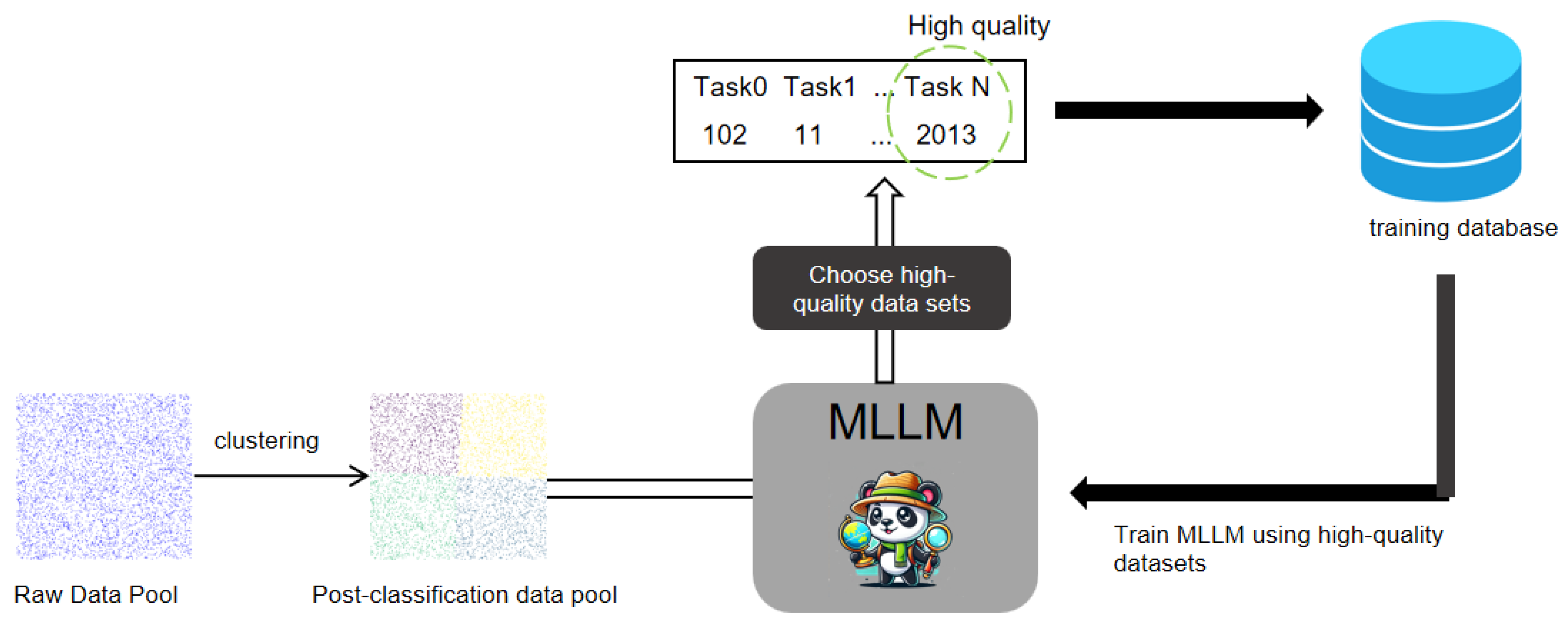
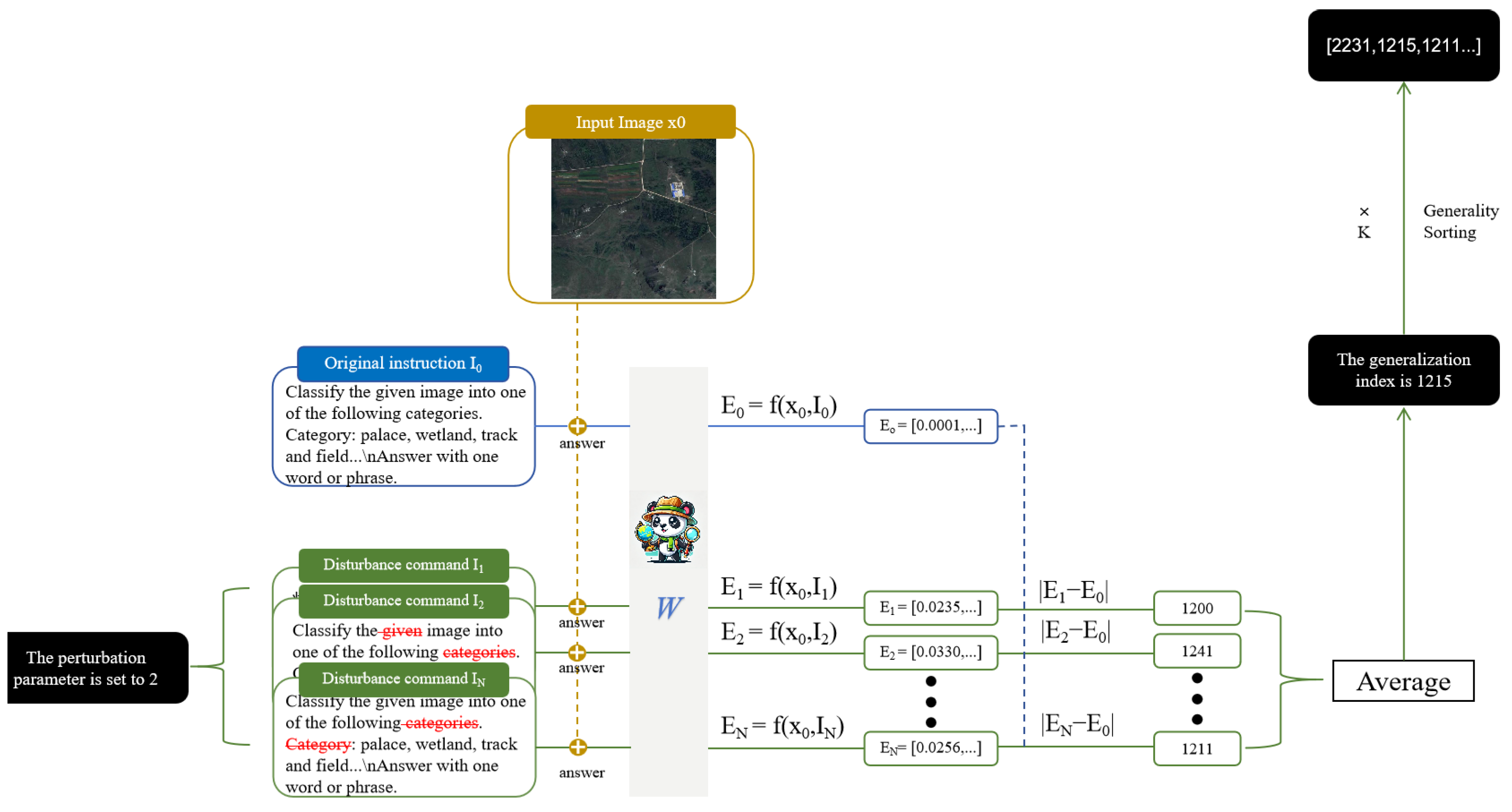
To address this gap, we proposed a novel, adaptive fine-tuning algorithm for multimodal large models, capable of automatically categorizing and filtering remote sensing multimodal instruction datasets to identify high-quality data for training from massive remote sensing datasets. The core steps of the algorithm include projecting the large-scale data into a semantic vector space and using the MiniBatchKMeans algorithm for automated clustering. Each data cluster was then processed by introducing perturbation parameters to the original data and calculating the translational differences between the original and perturbed data in the multimodal model’s vector space. This difference served as a generalization performance metric, determining the quality of the dataset. Finally, through a layer of ranking, we selected the batch of datasets with the highest generalization performance metrics for training.

We utilized the RS multimodal instruction-following dataset proposed by GeoChat for training and adopted the Evaluation Benchmark from GeoChat along with MMBench_DEV_EN [36], MME [37], and SEEDBench_IMG [38] as evaluation datasets for domain-specific and general domains, respectively. Through comparisons with random selection, the WaveCoder algorithm, and our proposed algorithm on the GeoChat classification dataset, our results demonstrated that our algorithm outperformed other baseline methods, maximizing domain capability enhancement while preserving generalization ability. Additionally, our algorithm’s selected one-third dataset reduced training time by approximately two-thirds compared to training on the entire dataset, with only a 1% average decrease in performance in the remote sensing domain, while significantly maintaining generalization capability. 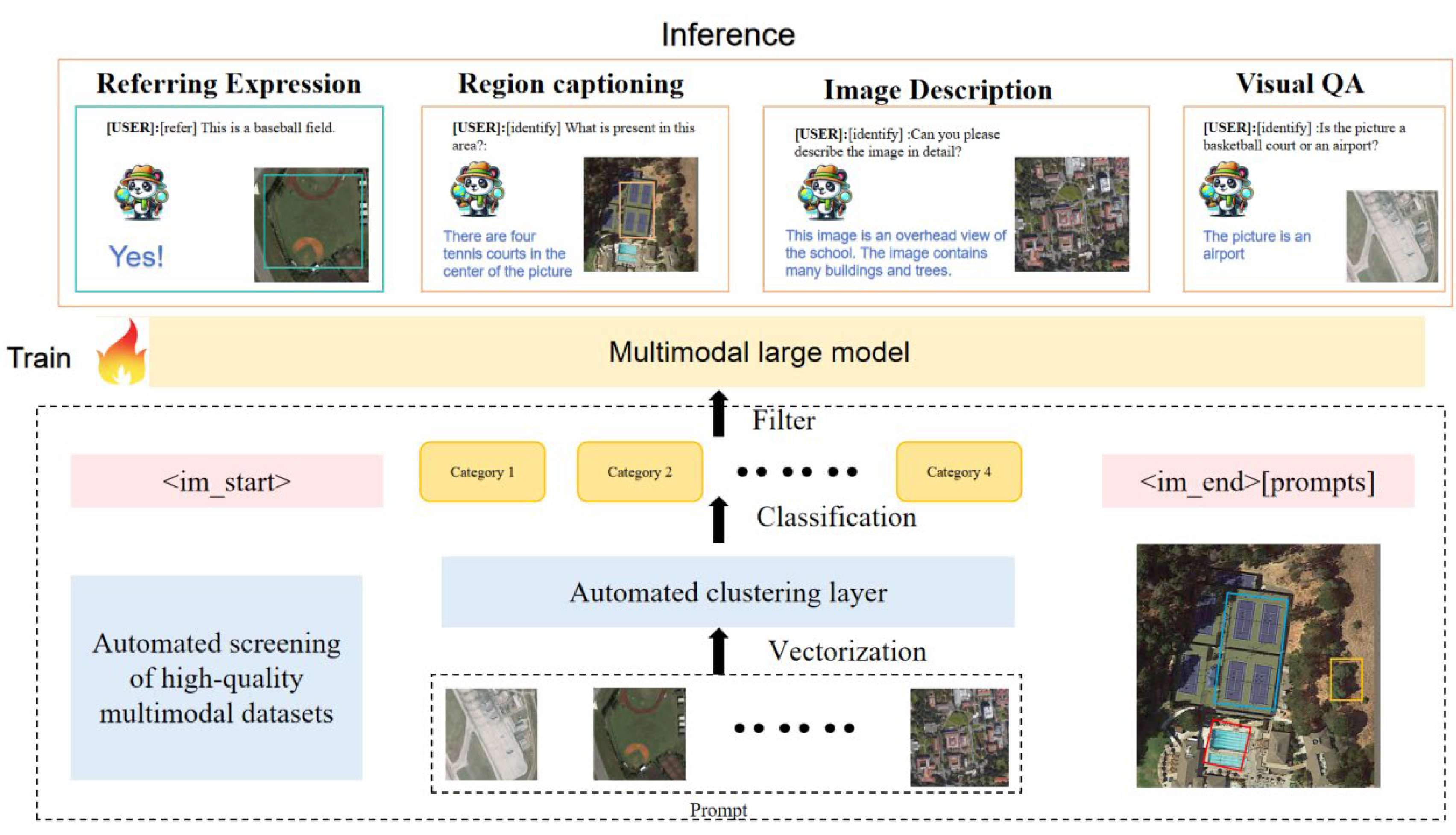Figure 1 illustrates our multimodal model’s versatility on six key remote sensing tasks by centering a single high-resolution aerial image and surrounding it with colored panels that pair user prompts and model responses for grounded image captioning, visual question answering, referring expression comprehension, scene classification, region-based captioning, and multi-turn conversation—demonstrating how the model seamlessly fuses visual and textual cues to describe scenes, count and localize objects, classify content, and engage in interactive dialog.

The main contributions of this paper are as follows:

• We proposed a new multimodal instruction fine-tuning dataset quality metric—generalization performance metric.
• We introduce a novel algorithm that selects high-quality remote sensing multimodal fine-tuning datasets to achieve faster and more efficient training results.
• By training on small datasets, we compared the effects of baseline algorithms and our algorithm in both general and remote sensing domains, validating that our algorithm achieved favorable results in the remote sensing domain.

2. Dataset Creation

2.1. Training Data

The RS multimodal instruction-following dataset is a multimodal instruction-following dataset designed for remote sensing image understanding. It integrates various tasks such as image description, visual question answering, and visual dialogue, aiming to enhance the model’s ability to handle complex reasoning, object attribute understanding, and spatial relationships. The dataset contains a total of 318,000 instruction pairs. The RS Multimodal Instruction-Following Dataset is a curated corpus of 318,000 high-quality instruction–response pairs aligned with 120,000 unique 256 × 256 px remote sensing image tiles, designed to support a unified multimodal instruction-following paradigm in the RS domain. These tiles were sourced from diverse satellite and aerial platforms, including Sentinel-2 MSI, Landsat-8 OLI, commercial sub-meter imagery, and Google Earth captures, covering a wide range of spatial resolutions (0.3 m to 10 m ground-sampling distance). The dataset generation pipeline leverages existing object-detection benchmarks to create initial image descriptions, then uses Vicuna-1.5 for LLM-driven conversation generation, and finally enriches the collection with visual question-answering and scene-classification examples drawn from dedicated RS datasets. By integrating tasks such as image captioning, VQA, object-attribute queries, spatial-relation reasoning, and multi-turn visual dialogue, it enables the comprehensive fine-tuning and evaluation of MLLMs for complex scene understanding in remote sensing. Hosted publicly on GeoX-Lab with full documentation and code, this dataset underpins state-of-the-art RS VLMs like GeoChat and RS-GPT4V, facilitating robust domain adaptation and zero-shot reasoning on unseen tasks.

2.2. Evaluation Datasets

Our evaluation datasets include two parts: the remote sensing evaluation dataset and the general multimodal evaluation dataset.

(1)

Remote Sensing Evaluation Datasets:

LRBEN (Land Use and Land Cover Remote Sensing Benchmark Dataset): This dataset is designed for land use and land cover classification tasks in remote sensing. It includes high-resolution images annotated for various types of land cover, such as urban areas, forests, water bodies, and agricultural fields. LRBEN is used to benchmark models’ performance in visual question answering, scene classification, and other tasks in remote sensing.

UC Merced Land Use Dataset: This dataset contains aerial imagery of various land use classes, such as agricultural, residential, and commercial areas. The images are high-resolution and cover 21 different classes, each with 100 images, making it suitable for scene classification tasks. It is widely used for evaluating remote sensing models’ ability to classify and understand different land use types.

AID (Aerial Image Dataset): AID is a large-scale dataset for aerial scene classification. It contains images from various scenes, such as industrial areas, residential areas, and transportation hubs. The dataset is designed to help in developing and benchmarking algorithms for scene classification, image retrieval, and other remote sensing tasks. AID includes a significant number of images for each category, providing a comprehensive benchmark for evaluating model performance.

(2)

General Multimodal Evaluation Datasets:

MMBench_DEV_EN: MMBench is a benchmark suite for evaluating the multimodal understanding capabilities of large vision-language models (LVLMs). It contains approximately 2974 multiple-choice questions covering 20 capability dimensions. Each question is single-choice, ensuring the reliability and reproducibility of the evaluation results. MMBench uses a strategy called cyclic evaluation to more reliably test the performance of vision-language models.

MME (Multimodal Evaluation): MME is a comprehensive evaluation benchmark for large multimodal language models, aiming to systematically develop a holistic evaluation process. The MME dataset includes up to 30 of the latest multimodal large language models and consists of 14 sub-tasks to test the models’ perceptual and cognitive abilities. The MME data annotations are all manually designed to avoid potential data leakage issues that might arise from using public datasets.

SEEDBench_IMG: SEEDBench is an image dataset specifically designed for training and evaluating multimodal models. It contains high-quality image data with detailed annotations, suitable for various multimodal tasks such as image classification, object detection, and scene understanding. The SEEDBench dataset aims to assist researchers in developing and optimizing multimodal models by providing a comprehensive benchmark.

3. Methods

3.1. Adaptive Self-Tuning for Multimodal Models

In real-world scenarios, the volume of instruction fine-tuning data is often large and continually expanding, leading to increased training costs. Additionally, as the data volume grows, data conflicts also become more pronounced, often resulting in poorer training outcomes. To address this issue, we proposed a new algorithm that enables large models to autonomously select data to better adapt to domain-specific tasks. The core of this algorithm is to allow the model to independently identify the most generalizable task instructions, achieving optimal performance with a minimal amount of training data. The flowchart of this process is shown in Figure 2. The complete training and inference process of our algorithm is illustrated in Figure 3.

3.2. Selection of Generalizable Tasks

The autonomous selection of task instruction datasets with greater generalization has been a research hotspot. For instance, Sid-dhant and Lipton’s work on uncertainty-based active learning [39] provides significant insights.

Inspired by these studies, we proposed a new generalization measure: vector space translation difference. Since large models predict the next word based on context, changes in the context vector affect subsequent content generation. We evaluated the uncertainty of instructions by randomly deleting words from the instruction context as perturbation information and observing the degree of change in the model’s vector space. Generally, entries with stronger uncertainty yield better generalization effects after training. Specifically, the vector space translation difference measures the translation difference in the vector space of the model’s projection vectors when given complete and perturbed task instructions, assessing the generalization of the instruction. This quantifies the model’s responsiveness to uncertain instructions, enabling a better evaluation of the model’s generalization performance.

The detailed flowchart is shown in Figure 4, and the specific steps were as follows:

• For the massive data pool X, we used the bge-large-en-v1.5 [40] model to project each data entry into a vector space and then performed automated clustering using the MiniBatchKMeans algorithm. Specifically, we performed clustering calculations for different numbers of clusters using the MiniBatchKMeans algorithm, recorded the SSE (sum of squared errors) and silhouette coefficient for each cluster number, and selected the optimal number of clusters based on the highest silhouette coefficient. The data were eventually divided into p clusters. The specific steps were as follows:

(1)

Data projection onto vector space:

$${\mathrm{V}}_{\mathrm{i}}={\mathrm{BGE}(\mathrm{X}}_{\mathrm{i}})$$

(1)

Here, Xi represents the ith data item in the data pool and Vi represents the vector representation projected through the bge-large-en-v1.5 model.

(2)

Calculation of the sum of squared errors (SSE):

$$\mathrm{SSE}={\displaystyle \sum _{\mathrm{j}=1}^{\mathrm{p}}{\displaystyle \sum _{V_i\in C_j}{\left|\right|V_i-{\mu }_j\left|\right|}^2}}$$

(2)

Here, p represents the number of clusters, Cj denotes the jth cluster, and μj is the centroid of the jth cluster. Vi represents the vector belonging to the jth cluster. The SSE measures the sum of the distances between data points and their respective cluster centroids, serving as one of the indicators to evaluate clustering performance. A smaller SSE indicates that the points within a cluster are more tightly grouped. By plotting the SSE values for different numbers of clusters p, one can preliminarily assess the reasonable range for the number of clusters.

(3)

Calculation of the silhouette coefficient:

$$\mathrm{s}\left(\mathrm{i}\right)={\displaystyle \frac{\mathrm{b}\left(\mathrm{i}\right)-\mathrm{a}\left(\mathrm{i}\right)}{\max \left(\mathrm{a}\right(\mathrm{i}),\mathrm{b}(\mathrm{i}\left)\right)}}$$

(3)

Here, a(i) represents the average distance from data point i to all other points within the same cluster and b(i) represents the average distance from data point i to the nearest points in a different cluster. The silhouette coefficient C for the entire dataset is the average of the silhouette scores s(i) for all data points:

$$C={\displaystyle \frac{1}{\mathrm{n}}}{\displaystyle \sum _{i=1}^{n}s(i)}$$

(4)

Here, n represents the total number of data points.

(4)

Selection of the optimal number of clusters:

$$p=\arg \underset{k}{\max }C(k)$$

(5)

Here, C(k) represents the silhouette coefficient for different numbers of clusters k and p is the optimal number of clusters that maximize C(k).

2.

For the given p-th cluster and the K-th original instruction I₀, add a perturbation parameter n (i.e., the number of words randomly deleted from each instruction). Generate N perturbed instructions randomly, denoted as I₁ to I_N.

3.

Then, concatenate the input image X₀, answer with I₀ to I_N, and project them into the vector space of the multimodal large model, as shown in the following formula:

$${\mathrm{E}}_0={\mathrm{f}(\mathrm{x}}_0{,\mathrm{I}}_0{),\mathrm{E}}_1{=\mathrm{f}(\mathrm{x}}_0{,\mathrm{I}}_1) \dots { \mathrm{E}}_{\mathrm{n}-1}{=\mathrm{f}(\mathrm{x}}_0{,\mathrm{I}}_{\mathrm{n}-1}{) , \mathrm{E}}_{\mathrm{n}}{=\mathrm{f}(\mathrm{x}}_0{,\mathrm{I}}_{\mathrm{n}})$$

(6)

4.

For the instructions I₀ to I_N and their corresponding images and answers, calculate the Euclidean distances between the projection vectors E₀ to E_N and the perturbed vectors E₁ to E_N sequentially, as follows:

$${\left|\right|\mathrm{E}}_1-{\mathrm{E}}_0{\left|\right|}_2 \dots { \left|\right|\mathrm{E}}_{\mathrm{N}-1}-{\mathrm{E}}_0{\left|\right|}_2{, \left|\right|\mathrm{E}}_{\mathrm{N}}-{\mathrm{E}}_0{\left|\right|}_2$$

(7)

5.

Sum the Euclidean distances between the perturbed vectors E₁ to E_N and E₀. Then, calculate the average value as the generalization measure, where n represents the perturbation parameter value and K represents the K-th data entry.

$${\mathrm{S}}_{\mathrm{n},\mathrm{k}}={\displaystyle \frac{1}{\mathrm{N}}}{\displaystyle \sum _{i=1}^N\left|\right|E_i-E_0|{|}_2}$$

(8)

6.

Finally, sort each instruction in the p-th cluster by its generalization measure, with higher measures corresponding to higher training priority.

$${\mathrm{Sort}(\mathrm{S}}_{1,\mathrm{k}} \dots { ,\mathrm{S}}_{\mathrm{n},\mathrm{k}})$$

(9)

3.3. Selection of Optimal Disturbance Parameters

To select the optimal disturbance parameter n, we observed the relative embedding differences when adding different disturbance parameters to determine the best value for n (The process is shown in Figure 5).

The specific steps were as follows:

• First, for the given K-th original instruction I₀, we sequentially added random parameters from 1 to n, resulting in disturbed instructions I₁ to I_N.
• Then, we concatenated the input image X₀ and the answer with I₀ to I_n, respectively, and projected them into the vector space of the multimodal large model to obtain vectors E₀ to E_n. The formula is as follows:

  $${\mathrm{E}}_0={\mathrm{f}(\mathrm{x}}_0{,\mathrm{I}}_0{),\mathrm{E}}_1{=\mathrm{f}(\mathrm{x}}_0{,\mathrm{I}}_1) \dots { \mathrm{E}}_{\mathrm{n}-1}{=\mathrm{f}(\mathrm{x}}_0{,\mathrm{I}}_{\mathrm{n}-1}{) , \mathrm{E}}_{\mathrm{n}}{=\mathrm{f}(\mathrm{x}}_0{,\mathrm{I}}_{\mathrm{n}})$$

  (10)
• For the obtained vectors E₀ to E_n, we sequentially calculated the Euclidean distance between each perturbed vector E₁ to En and the original vector E₀ to E_n. The formula is as follows:

  $${\left|\right|\mathrm{E}}_1-{\mathrm{E}}_0{\left|\right|}_2 \dots { \left|\right|\mathrm{E}}_{\mathrm{n}-1}-{\mathrm{E}}_0{\left|\right|}_2{, \left|\right|\mathrm{E}}_{\mathrm{n}}-{\mathrm{E}}_0{\left|\right|}_2$$

  (11)
• Then, we calculated the average embedding difference S_n,k for the K entries under the disturbance parameter n. We sequentially calculated the relative embedding differences D_n,K from 1 to n and selected the disturbance parameter with the maximum relative embedding difference as the optimal disturbance parameter. The formula is as follows, where K represents the p-th data pool containing K entries and n represents the disturbance parameter:

  $${\mathrm{S}}_{\mathrm{n},\mathrm{K}}={\displaystyle \sum _{i=1}^K\left|\right|{{\displaystyle E}}_{\mathrm{n}}^i-{{\displaystyle E}}_0^i|{|}_2}$$

  (12)

  $${\mathrm{D}}_{\mathrm{n},\mathrm{k}}={\mathrm{S}}_{\mathrm{n},\mathrm{K}}-{\mathrm{S}}_{\mathrm{n}-1,\mathrm{K}}$$

  (13)

  $$n=P(n|Max({\mathrm{D}}_{1,\mathrm{K}},\dots {\mathrm{D}}_{\mathrm{n},\mathrm{K}}))$$

  (14)

3.4. Compare Algorithms

Algorithm 1: Random Sampling

The random sampling method involves randomly selecting a subset of the dataset for training. This approach often captures the most diverse and broadly representative data from the dataset. Therefore, we used the random sampling algorithm as our baseline for comparison.

Algorithm 2: KCenterGreedy Clustering Algorithm

WaveCoder proposes a method for selecting a core dataset using the KCenterGreedy clustering algorithm. In this approach, we used the bge-visualized-m3 [41] model to project each image-text pair into vector space. We then applied the KCenterGreedy algorithm for clustering and selected a representative subset of the dataset.

4. Results

4.1. Training Details

We performed LoRA [42] fine-tuning on the InternLM-XComposer2-VL-7B [43] model using the RS multimodal instruction-following dataset. The fine-tuning parameters are shown in

Table 1. Training parameters.

Hyper Parameter	Value
Precision	fp16
Epochs	3
Maximum context length	4096
Batch size	8
Weight_decay	0.1
Warmup_ratio	0.01

.

4.2. Experiment on Disturbance Parameter Settings

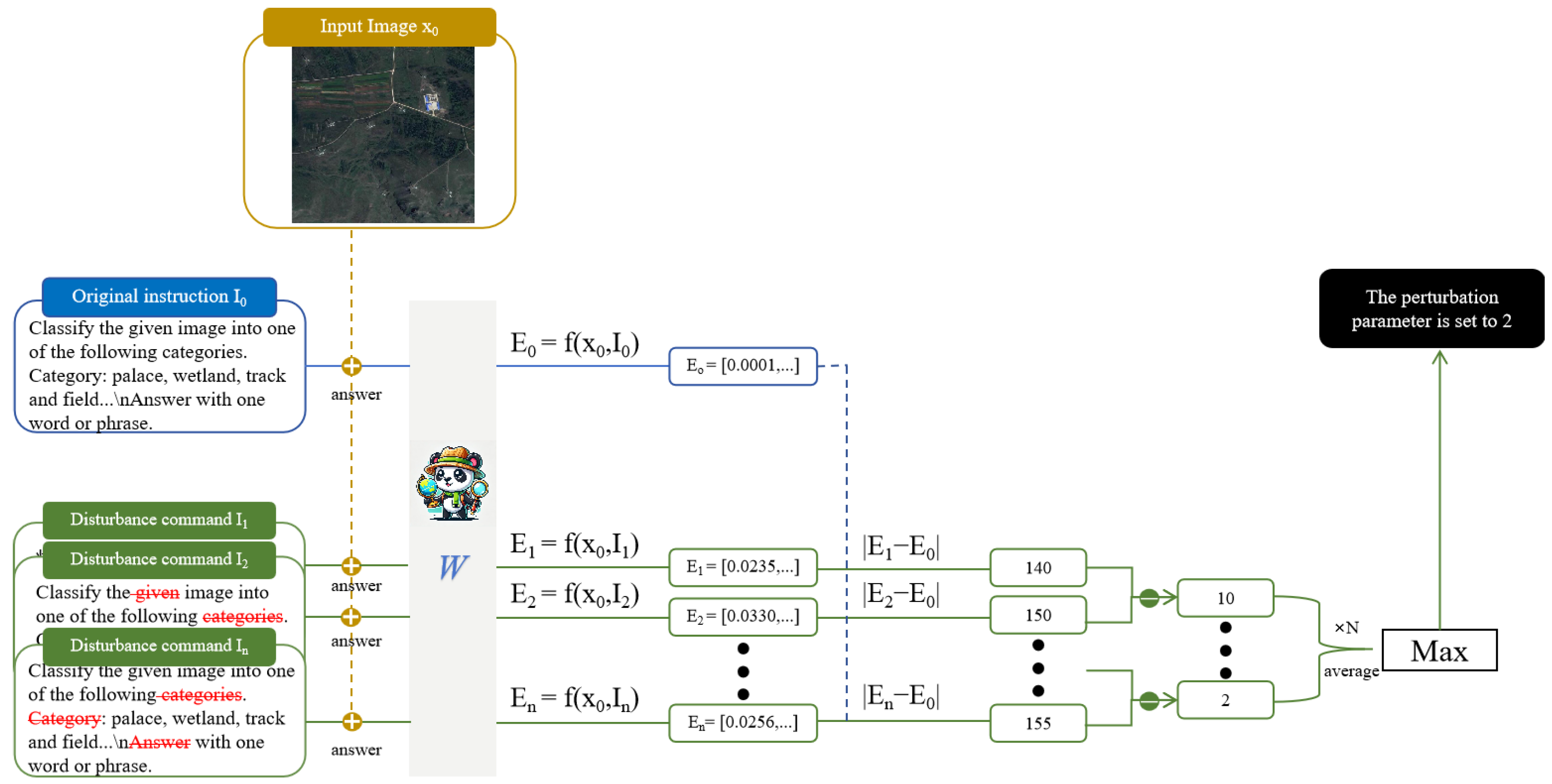
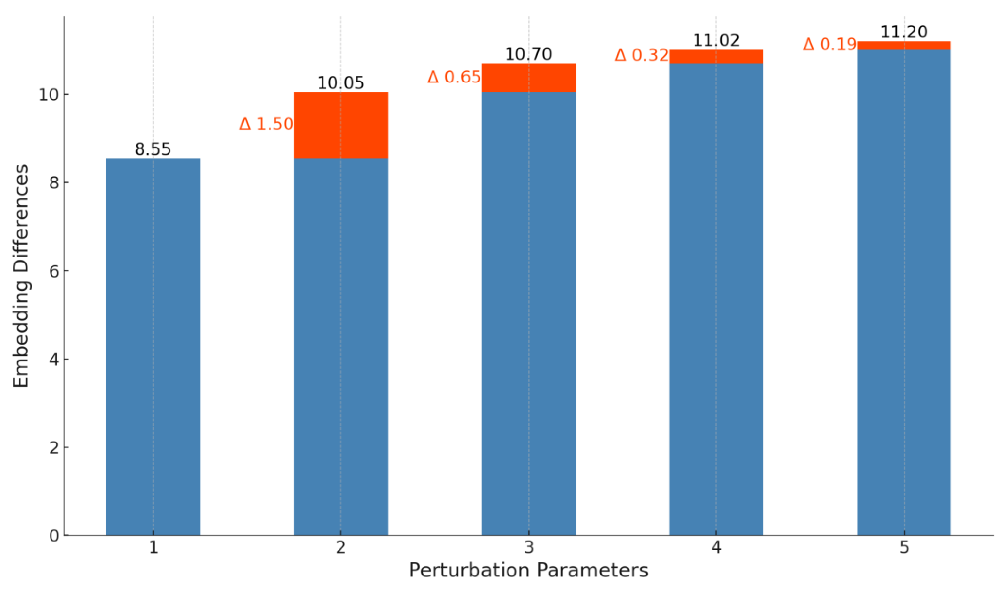
To validate the effectiveness of our algorithm, we used a subset of clustered data focused on classification tasks, containing 32 k entries, as the training set. We first evaluated the optimal disturbance parameter using our algorithm, and the relative vector embedding differences are shown in Figure 6.

As shown in the figure, the optimal disturbance parameter was 2, with the value gradually converging and the change magnitude decreasing, approaching 0 after 4.

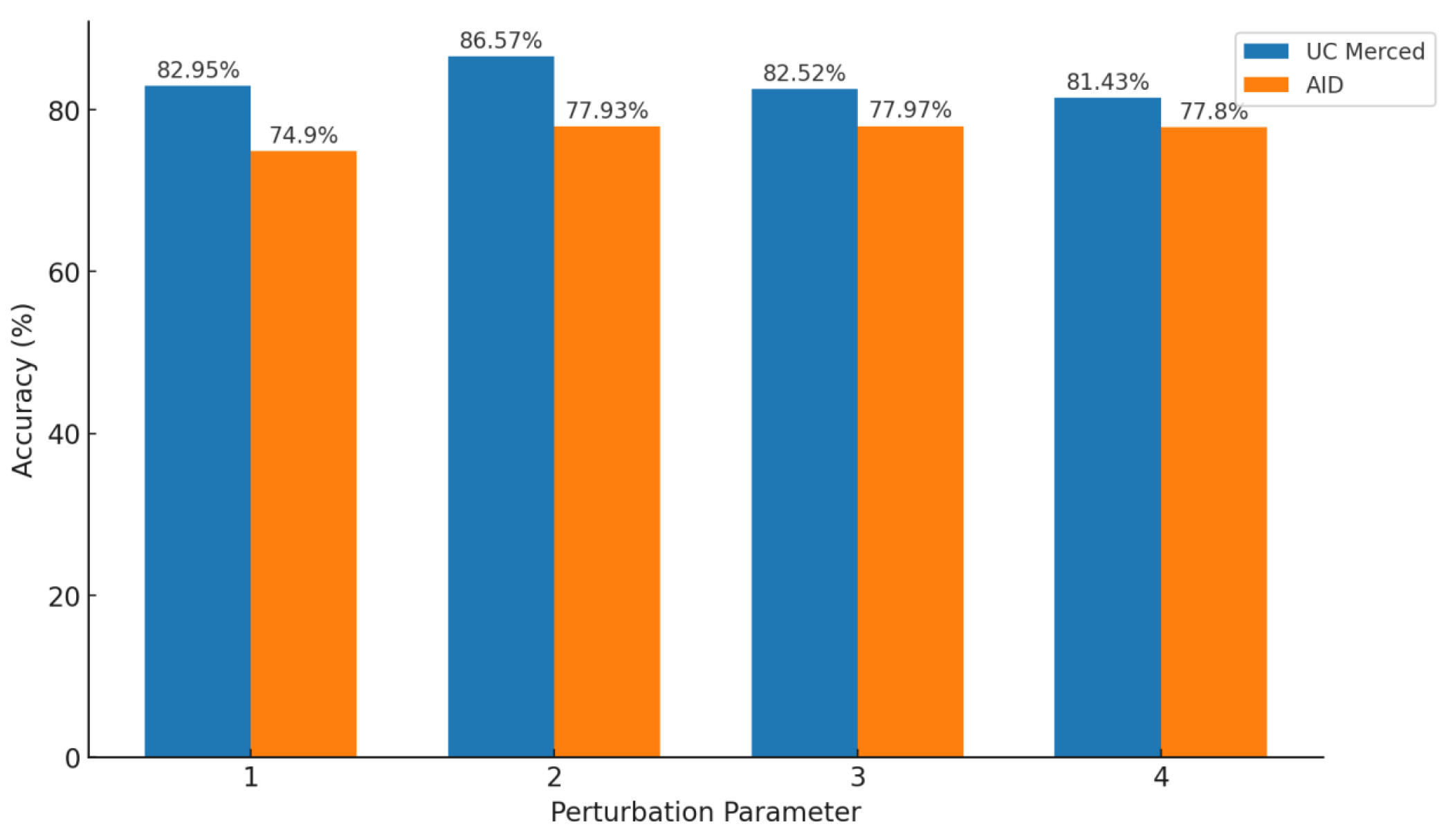
Therefore, we set the optimal disturbance parameter to 2. To further verify this, we used our algorithm to rank the generalizability of the training set with disturbance parameters from 1 to 4. We selected the top 5000 entries with the highest generalizability for training and evaluated the performance on the UC Merced and AID datasets. The results are shown in Figure 7.

From the figure, the model achieved the best training performance when the disturbance parameter was set to 2, reaching 86.57% accuracy on the UC Merced dataset—4 percentage points higher than with a parameter of 1 or 3. On the AID dataset, it attained 77.93%, only 0.04 percentage points below the peak value at n = 3. Additionally, we conducted experiments on two other clusters of 25 K and 90 K entries. Using our algorithm, we selected 5 K samples from each cluster for training. The evaluation results in

Table 2. Model performance on RSVQA-LR when trained on 5 K samples selected by our algorithm from a 25 K entry cluster under varying perturbation parameter n.

Model/n	RSVQA-LR
	Rural/Urban	Presence	Compare	Avg.
InternLM-XComposer2-VL-7B	69.00	52.62	70.80	64.14
Ours (1)	71.00	84.81	77.24	77.68
Ours (2)	71.00	85.45	78.57	78.57
Ours (3)	69.00	83.76	79.89	77.55
Ours (4)	73.00	83.52	79.11	78.54

and

Table 3. Model performance on AID and UC Merced when trained on 5 K samples selected by our algorithm from a 90 K entry cluster under varying perturbation parameter n.

Model/n	AID	UC Merced	Avg.
InternLM-XComposer2-VL-7B	62.87	65.38	64.13
Ours (1)	72.88	82.71	77.80
Ours (2)	74.93	83.45	79.19
Ours (3)	73.12	83.21	78.17
Ours (4)	73.00	82.52	77.76

confirmed that, with n = 2, the models achieved optimal performance on RSVQA-LR, AID, and UC Merced. Overall, the model’s best training performance was obtained when the disturbance parameter was set to 2.

4.3. Optimal Training Data Ratio

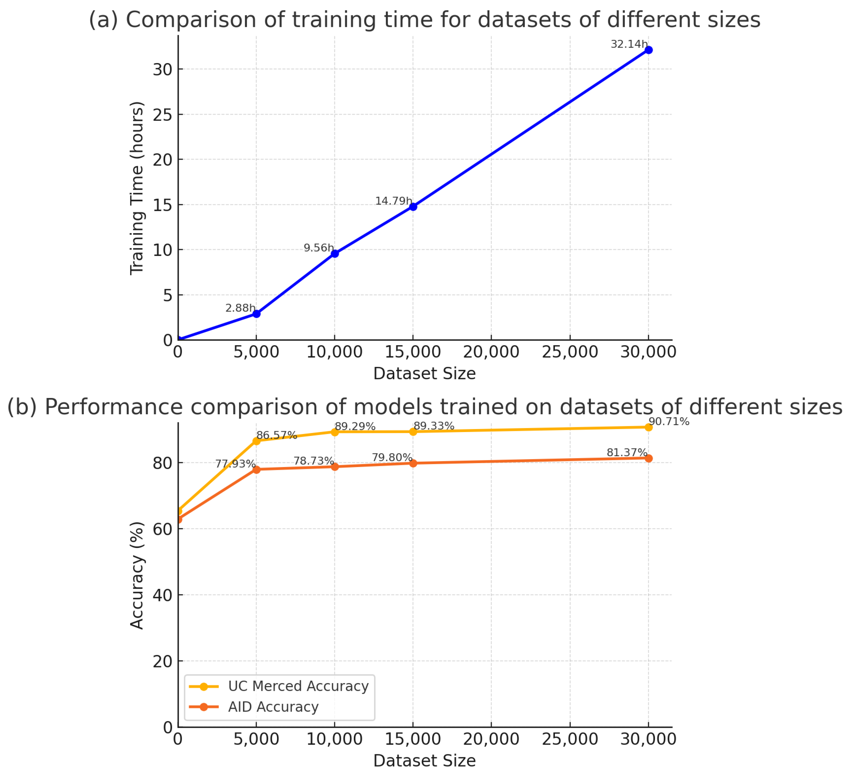
To determine the optimal training data ratio, we conducted a detailed comparison of training durations and model performance for different data volumes (5000, 10,000, 15,000, and 32,000 samples). The experimental results are shown in Figure 8.

As illustrated in Figure 8, increasing the training data volume led to improved model performance on both the AID and UC Merced datasets. Specifically, with 5000 samples, the performance on the AID dataset was 77.93, and on the UC Merced dataset, it was 86.57. When the data volume was increased to 10,000 samples, the performance on the AID and UC Merced datasets rose to 78.73 and 89.29, respectively. Further increasing the data volume to 15,000 and 32,000 samples resulted in performance levels of 79.80 and 81.37, as well as 89.33 and 90.71. This indicates that more data generally improve model performance, but the performance gain gradually diminishes.

The training duration data showed a significant increase with the data volume. For instance, training with 5000 samples took 2.88 h, while training with 32,000 samples increased to 32.14 h, an additional 29.26 h.

By comparing model performance and training durations across different data volumes, we found that with 10,000 samples, the model’s performance was close to its peak, while the training duration was significantly lower compared to 15,000 and 32,000 samples. Specifically, the performance difference between 10,000 and 32,000 samples was an average of 2.13, with a reduction in computation cost by 22.18 h.

In summary, with 10,000 samples, the model achieved a high performance while significantly reducing training time and computational resources. Thus, 10,000 samples represent the optimal balance between performance and computational cost. This indicates that using approximately one-third of the total dataset achieves better training results while substantially lowering the computational cost.

4.4. Comparison of Algorithm Performance

To further validate the effectiveness of our algorithm, we compared random sampling, the KCenterGreedy clustering algorithm, and our algorithm. We selected 5000 data entries for training in each case and compared the model’s performance on the UC Merced and AID datasets. The results are shown in

Table 4. Comparison of training effects of different algorithm models under 5000 pieces of data.

Train Type	AID	UC Merced	Avg.
Baseline (random)	77.43	85.90	81.67
KCenterGreedy	78.07 ↑ 0.64	82.00 ↓ 3.90	80.04 ↓ 1.63
Ours	77.93 ↑ 0.50	86.57 ↑ 0.67	82.25 ↑ 0.58

(In the table below, we use red text to indicate the extent of decreases and green text to indicate the extent of increases).

As shown in the table, our algorithm improved the baseline algorithm (random sampling) by 0.50 on the UC Merced dataset and 0.67 on the AID dataset, with an average improvement of 0.58. In contrast, the KCenterGreedy clustering algorithm improved by 0.64 on the UC Merced dataset but decreased by 3.90 on the AID dataset, resulting in an overall decrease of 1.63 compared to the baseline algorithm. Overall, our algorithm achieved the best training performance.

To further observe the improvement of our algorithm over the baseline algorithm, we tested the training performance on a dataset of 10,000 entries and on the entire classification dataset. The results are shown in

Table 5. Comparison of training effects of different algorithm models under different scales of data.

Method	Size	AID	UC Merced	Avg.
Baseline (random)	10 k	78.10	87.52	82.81
Ours	10 k	78.73 ↑ 0.63	89.29 ↑ 1.77	84.04 ↑ 1.20
Direct	32 k	81.37 ↑ 3.27	90.71 ↑ 3.19	86.04 ↑ 3.23

.

As shown in the table, when the dataset size was expanded to 10,000 entries, our algorithm showed even greater advantages, improving by 0.63 on the AID dataset and by 1.77 on the UC Merced dataset compared to the baseline algorithm, with an overall improvement of 1.20. The average improvement of 0.58 from 5000 to 10,000 entries was nearly double, indicating that the performance improvement brought by our algorithm increased with the dataset size. Additionally, when training on the entire 32 k dataset, our algorithm, using only 10 k entries, was only 1.42 points lower on the UC Merced dataset and 2.64 points lower on the AID dataset, with an overall average decrease of 2.00. This result demonstrates that our algorithm can significantly approximate the performance of training on the entire dataset with just one-third of the data.

Furthermore, we compared the performance of models trained with our algorithm and the baseline algorithm in general domains. The results are shown in

Table 6. Comparison of general performance of different algorithm models under different scales of data.

Method	Model	Size	MMBench	SEEDBench	MME
/	InternLM-XComposer2-VL-7B	/	83.97	75.9	2242.70
Baseline (random)	InternLM-XComposer2-VL-7B	10 k	84.22 ↑ 0.25	75.13 ↓ 0.77	2272.01 ↑ 29.31
Ours	InternLM-XComposer2-VL-7B	10 k	84.38 ↑ 0.41	75.45 ↓ 0.45	2276.30 ↑ 33.60
Direct	InternLM-XComposer2-VL-7B	32 k	84.57 ↑ 0.60	75.14 ↓ 0.76	2245.15 ↑ 2.450

.

As shown in the table, our algorithm also retained the best general domain capabilities, demonstrating superior performance over the random sampling method on the MMBench_DEV_en, SEEDBench, and MME datasets, achieving scores of 84.38, 75.45, and 2276.30, respectively. The performance on MMBench_DEV_en and SEEDBench exceeded that of the original model, with improvements of 0.41 and 33.60, respectively. In contrast, while direct training on the 32 k dataset showed an improvement on MMBench_DEV_en, it slightly declined on SEEDBench. Overall, our method significantly enhanced performance metrics in the remote sensing domain while maintaining the model’s general capabilities, demonstrating its effectiveness and superiority.

4.5. Final Performance of Our Algorithm

Using our algorithm for automatic clustering, we divided the RS multimodal instruction-following dataset into seven categories, as shown in the vector space visualization in Figure 9.

We then selected 15,000 data entries from each category, totaling 105,000 entries for training. The model was trained for three epochs, and the results are shown in

Table 7. Comparing the evaluation results of different models on AID and UC Merced datasets.

Model	AID	UCMerced	Avg.
MiniGPTv2 [44]	4.76	12.90	8.83
Qwen-VL-Chat [45]	62.90	52.60	57.75
LLaVA-1.5 [46]	68.00	51.00	59.5
InternLM-XComposer2-VL-7B	62.87	65.38	64.13
GeoChat	72.03	84.43	78.23
Ours	77.19	89.86	83.53

We highlighted our trained model’s results in bold.

and

Table 8. Comparing the evaluation results of different models on the LRBEN dataset.

Model	RSVQA-LR
	Rural/Urban	Presence	Compare	Avg.
LLaVA-1.5	59.22	73.16	65.19	65.86
InternLM-XComposer2-VL-7B	69.00	52.62	70.80	64.14
MiniGPTv2	60.02	51.64	67.64	59.77
InstructBLIP [47]	62.62	48.83	63.92	59.12
Mplug-Owl2 [48]	57.99	74.04	65.04	65.69
Qwen-VL-Chat	62.00	47.65	54.64	58.73
SkyEyeGPT [49]	88.93	88.63	75.00	84.16
RSGPT	94.00	91.17	91.70	92.29
GeoChat	91.09	90.33	94.00	91.81
LHRS-Bot [50]	89.07	88.51	90.00	89.19
Ours	89.00	91.91	91.78	90.90

We highlighted our trained model’s results in bold.

.

As shown in Table 7 and Table 8, we highlighted our trained model’s results in bold. The model trained with only 105 k entries achieved 77.19 on the AID dataset and 89.86 on the UC Merced dataset, which are 5.16 and 5.43 points higher than GeoChat, respectively. On the LRBEN dataset, it achieved an average of 90.90, only 0.91 points lower than GeoChat. Observing the performance of the original models on the AID, UC Merced, and LRBEN datasets, we find that our original model InternLM-XComposer2-VL-7B outperformed GeoChat’s original model LLaVA-1.5 by an average of 4.63 on AID and UC Merced. After training, our model outperformed GeoChat by 5.3 on these datasets. On the LRBEN dataset, InternLM-XComposer2-VL-7B scored 1.72 points lower than LLaVA-1.5, and our final trained model scored 0.91 points lower than GeoChat.

These results indicate that the performance of the original model has a direct positive impact on the final training performance. However, the key finding is that by selecting high-quality, generalizable datasets, our algorithm can achieve results comparable to those obtained from training on the full dataset, using only one-third of the data. This demonstrates the effectiveness and efficiency of our method in enhancing model performance.

4.6. Ablation Study

4.6.1. Rationale for the Generalization Measure

We treat the embedding shift after word deletion as a generalization metric because the instruction fine-tuning stage primarily serves to activate the model’s capabilities. When we randomly delete words from an instruction, the greater the change in the model’s understanding is and the more critical the lost information is. By performing multiple random deletions and averaging the resulting shifts, this approach more accurately identifies which samples the model considers to contain the most key information—and, thus, which will yield the greatest training benefit. As shown in

Table 9. Instructions with highest and lowest generalization measures in a classification cluster.

Instruction	Score	Difficulty (1–10)
Is there a rectangular building? \nAnswer in one word or a short phrase.	4.4453125	3—Only needs to detect a single object; logic is simple.
Are there more large forests than buildings? \nAnswer in one word or a short phrase.	1603.390234375	5—Requires comparing counts of two classes; slightly more reasoning.

, we listed the instructions with the highest and lowest generalization measures within a cluster for a classification task. We then used GPT-O3 to rate each instruction’s difficulty and found that higher-generalization instructions tend to be more challenging. From that cluster, we extracted the 100 samples with the highest generalization measures and the 100 with the lowest and tested them using the original InternLM-XComposer2-VL-7B model. As

Table 10. InternLM-XComposer2-VL-7B accuracy on high- vs. low-generalization instruction samples.

Level	Number	Accuracy (%)
Low	100	64
High	100	33

demonstrates, samples with higher generalization measures produce higher model accuracy—and training on more difficult instructions delivers greater performance improvements.

4.6.2. Comparison of Different Perturbation Methods

We carried out further experiments to compare how different perturbation strategies affect our algorithm. Specifically, we applied two-word swaps and direct Gaussian-noise injection (mean = 0, standard deviation = 0.001) into the embedding vectors. We then trained on 5 K randomly sampled examples from a cluster containing 32 K items. The resulting model performances are presented in

Table 11. Model performance comparison under word deletion, word swap, and Gaussian-noise perturbations.

Perturbation Method	AID	UC Merced	Avg.
Base model	62.87	65.38	64.13
Swap words (2 word pairs)	73.97	71.62	72.80
Add perturbation vector	72.17	75.43	73.80
Delete words (2 words)	77.93	86.57	82.25

. As shown, deleting words at random yielded the best performance; both swapping words and adding noise to the embeddings performed substantially worse. We attribute this to the fact that swapping words rarely removes truly critical information and that small Gaussian perturbations in the embedding space do not induce sufficiently large changes. In contrast, word deletion provides a simple and effective way to alter the model’s interpretation of the instruction.

4.6.3. Impact of the Clustering Module

To evaluate how the clustering step affected our selection algorithm, we treated the 32 K example cluster as Cluster 0 and the 25 K example cluster as Cluster 1. We then applied our algorithm to each cluster separately to sample 5 K examples for training. The results are reported in

Table 12. AID and UC Merced performance for 5 K samples from Cluster 0 vs. Cluster 1.

Cluster	AID	UC Merced	Avg.
Base model	62.87	65.38	64.13
Clus 0	77.93	86.57	82.25
Clus 1	61.43	62.62	62.025

and

Table 13. RSVQA-LR performance for 5 K samples from Cluster 0 vs. Cluster 1.

Cluster	RSVQA-LR
	Rural/Urban	Presence	Compare	Avg.
Base model	69.00	52.62	70.80	64.14
Clus 0	67.00	46.80	70.21	61.34
Clus 1	71.00	85.45	78.57	78.57

. Data drawn from Cluster 0 yielded a large performance gain on AID and UC Merced—from 64.13% up to 82.25%—but a slight drop on RSVQA-LR (64.14% → 61.34%). Conversely, data from Cluster 1 boosted RSVQA-LR markedly (64.14% → 78.57%) while causing the AID and UC Merced scores to fall (64.13% → 62.03%). This confirms that the clustering effectively grouped samples by their dominant semantic tasks.

We then carried out two further experiments:

• Mixed-Subsets Training—merge the two 5 K subsets (one from each cluster) and train on the 10 K combined set.
• Merge-then-Select—first merge all 57 K examples, sample 10 K with our algorithm, and train.

Results (

Table 14. AID and UC Merced performance for Cluster-then-Select vs. Merge-then-Select Training.

Type	AID	UC Merced	Avg.
Base model	62.87	65.38	64.13
Cluster-then-Select	77.00	83.52	80.26
Merge-then-Select	77.50	83.67	80.59

and

Table 15. RSVQA-LR Performance for Cluster-then-Select vs. Merge-then-Select Training.

Type	RSVQA-LR
	Rural/Urban	Presence	Compare	Avg.
Base model	69.00	52.62	70.80	64.14
Cluster-then-Select	67.00	85.55	79.49	77.35
Merge-then-Select	69.00	85.04	79.89	77.98

) showed that, across RSVQA-LR, AID, and UC Merced, the Cluster-then-Select approach (sampling 5 K per cluster) consistently outperformed both mixed-subsets and merge-then-select strategies. Moreover, training on the mixed dataset always incurs a performance penalty compared to training on each cluster’s 5 K subset.

4.6.4. Algorithm Efficiency Comparison

We measured both the training time and the required GPU memory for our method and the two baselines. The results are summarized in

Table 16. Computational time and GPU memory usage comparison for random sampling, our algorithm, and KCenterGreedy.

Type	Time Complexity	Memory
Ours	O (n)	O (1)
Random	O (nD + nS)	O (d)
KCenterGreedy	O (nE)	O (e)

, where:

• D is the time for the embedding model to process one sample;
• S is the size of the selected core subset;
• E is the time to obtain a single multimodal-model embedding;
• D is the GPU memory used by the embedding model;
• E is the GPU memory used by the multimodal model.

As the table shows, random sampling had the lowest cost in both time and memory but it did not achieve the best training performance. Our algorithm came next in computational cost, while KCenterGreedy was the most expensive. Regarding memory usage, our method usually requires the most, followed by KCenterGreedy, with random sampling again being the cheapest.

To further evaluate the performance of our algorithm, we compared the results of training on the entire dataset versus a 105 k subset selected by our algorithm, both using InternLM-XComposer2-VL-7B on two 3090 GPUs for one epoch. The results are shown in

Table 17. Comparing the evaluation results of models trained on datasets of different scales on AID and UC Merced.

Method	Size	AID	UC Merced	Avg.
Ours	105 k	75.60	85.67	80.64
Random	105 k	73.21	83.45	78.33
KCenterGreedy	105 k	72.30	83.63	77.82
Direct	318 k	75.07 ↓ 0.53	87.95 ↑ 2.28	81.51 ↑ 0.87

,

Table 18. Comparing the evaluation effects of models trained on datasets of different scales on LRBEN.

Method Ours	RSVQA-LR
	Rural/Urban	Presence	Compare	Avg.
Ours	90.00	90.73	91.05	90.59
Random	88.00	89.52	90.03	89.18
KCenterGreedy	89.00	87.54	90.42	88.99
Direct	92.00 ↑ 2.00	91.57 ↑ 0.84	92.45 ↑ 1.40	92.01 ↑ 1.42

and

Table 19. Comparing the evaluation effects of models trained on datasets of different scales in general fields.

Method	Model	Size	MMBench	SEEDBench	MME
/	InternLM-XComposer2-VL-7B	/	83.97	75.9	2242.70
Ours	InternLM-XComposer2-VL-7B	105 k	83.78 ↓ 0.19	74.92 ↓ 0.98	2121.01 ↓ 121.69
Random	InternLM-XComposer2-VL-7B	105 k	83.72 ↓ 0.25	74.22 ↓ 1.68	2013.02 ↓ 229.68
KCenterGreedy	InternLM-XComposer2-VL-7B	105 k	83.64 ↓ 0.33	74.35 ↓ 1.55	2105.07 ↓ 137.63
Direct	InternLM-XComposer2-VL-7B	318 k	83.75 ↓ 0.22	74.18 ↓ 1.72	1982.90 ↓ 259.80

. Notably, training on the 105 k dataset took approximately 35 h, while training on the full 318 k dataset required around 110 h, more than three times the time consumption.

As shown in Table 7 and Table 8, our algorithm outperformed both random sampling and the KCenterGreedy method in every evaluation, and—for remote sensing tasks—using the full training set offered virtually no advantage over the one-third subset selected by our approach. On the AID benchmark, the subset model even attained an accuracy that was 0.53 percentage points higher than the model trained on all available data. We believe this occurred because, in multi-task scenarios with highly diverse samples, merely enlarging the dataset also enlarges the pool of conflicting or redundant examples. These conflicts can introduce gradient noise and hinder optimization. Our selection algorithm mitigated this issue by filtering out samples that contribute little new information or that clash with other tasks, thus yielding a cleaner training signal and more reliable performance despite—or even because of—the reduced data volume. Our algorithm reached an accuracy of 80.64 on the AID and UC Merced evaluation datasets, which was only 0.87% lower than training on the full dataset. On the RSVQA-LR dataset, our algorithm averaged an accuracy of 80.59, just 1.42% lower than the full dataset training.

It is worth noting that the training results on the UC Merced and AID datasets were not as high as those achieved by training on a single type of dataset, as described in Section 4.3. This indicates that training on datasets of different types together can lead to significant data conflicts. However, our method achieved a higher score on the AID dataset compared to training on the entire dataset, suggesting that selecting high-quality subsets can alleviate some of the data conflicts.

It is worth noting that, in general-domain tasks, our algorithm retained better performance than training directly on the full dataset, achieving scores of 83.78, 74.92, and 2121.01 on MMBench, SEEDBench, and MME, respectively—all higher than the performance scores of the model trained on the full dataset. Additionally, on the SEEDBench and MME datasets, the accuracy loss from training on the full dataset was nearly twice that of the loss from our algorithm.

In summary, our algorithm saves more than twice the training time while maximizing the retention of general-domain capabilities, with only about a 1% accuracy loss in the remote sensing domain.

5. Conclusions

This study addresses the issue of data selection for multimodal large models in various domain tasks by proposing an adaptive fine-tuning algorithm. Most current research directly trains on large-scale multimodal data, which not only require substantial computational resources but also result in significant performance degradation when randomly selecting a small subset of data. To resolve this, we first projected the large-scale data into vector space and used the MiniBatchKMeans algorithm for automated clustering. Then, we measured the generalizability of the data by calculating the translation difference in the multimodal large model’s vector space between the original and perturbed data and autonomously selected data with high generalizability for training.

Our experiments, based on the InternLM-XComposer2-VL-7B model, were conducted on the remote sensing multimodal dataset proposed by GeoChat. The results show that using the adaptive fine-tuning algorithm, our method outperforms the random sampling and KCenterGreedy clustering algorithms in training with a 5000-entry dataset, achieving the best domain and general performance with a 10,000-entry dataset. Ultimately, using only 105,000 data entries—one-third of the GeoChat dataset—and training on a single 3090 GPU, our model achieved performances of 89.86 on the UC Merced dataset and 77.19 on the AID dataset, which are 5.43 and 5.16 points higher than GeoChat, respectively. On the LRBEN evaluation dataset, our model was only 0.91 points lower on average. Furthermore, comparing the performance of models trained on the full dataset versus our one-third dataset, we found that our approach reduced training time by more than 68.2% while maintaining general-domain capabilities with only a 1% average decrease in remote sensing accuracy.

In summary, our adaptive fine-tuning algorithm effectively selects high-quality data, enhancing model performance in specific domains while maintaining general performance under limited computational resources. This algorithm has significant practical value for training multimodal large models, especially in scenarios with constrained computational resources.

Nevertheless, our approach still has several limitations: (1) because the perturbation strategy relies on randomly deleting words, it may occasionally remove critical terms and thus underestimate the generalizability of some short or jargon-heavy instructions; (2) the embedding step depends on a large encoder, which limits deployment on edge devices with very restricted GPU memory; and (3) the method has been validated only on a remote sensing corpus, so its effectiveness in other multimodal domains remains to be systematically verified.