Enhancing Aquifer Reliability and Resilience Assessment in Data-Scarce Regions Using Satellite Data: Application to the Chao Phraya River Basin

Abstract

There are serious ecological and environmental risks associated with groundwater level decline, particularly in areas with little in situ monitoring. In order to monitor and assess the resilience and dependability of groundwater storage, this paper proposes a solid methodology that combines data from land surface models and satellite gravimetry. In particular, the GRACE Groundwater Drought Index (GGDI) is used to analyze the estimated groundwater storage anomalies (GWSA) from the Gravity Recovery and Climate Experiment (GRACE) and the Global Land Data Assimilation System (GLDAS). Aquifer resilience, or the likelihood of recovery after stress, and aquifer reliability, or the long-term probability of remaining in a satisfactory state, are calculated using the core method. The two main components of the methodology are (a) calculating GWSA by subtracting the surface and soil moisture components from GLDAS, total water storage from GRACE, and comparing the results to in situ groundwater level data; and (b) standardizing GWSA time series to calculate GGDI and then estimating aquifer resilience and reliability based on predetermined threshold criteria. Using this framework, we validate GRACE-derived GWSA with in situ observations in eight sub-basins of the Chao Phraya River (CPR) basin, obtaining Pearson correlation coefficients greater than 0.82. With all sub-basins displaying values below 35%, the results raise significant questions about resilience and dependability. This method offers a framework that can be applied to assessments of groundwater sustainability worldwide.

1. Introduction

Aquifer systems are pivotal in global hydrological and biogeochemical cycles, supporting the health of ecosystems [1,2,3,4]. Groundwater, an essential component of these systems, sustains the domestic, agricultural, and industrial needs of billions of people worldwide [5,6,7]. Despite their vital importance, groundwater levels are increasingly under threat from the combined effects of climate change and anthropogenic activities, leading to an estimated depletion of 41.4 km³/year from 1900 to 2008 [8,9,10]. This decline poses threats to water security, impacts the agricultural and energy sectors, and increases the risk of global conflicts.

Historically, groundwater assessment methodologies have relied heavily on in situ measurements. Although accurate, these methods are often spatially limited and logistically challenging, particularly in large or inaccessible regions [11,12]. Traditional approaches, such as well-based monitoring and hydrological modeling, require extensive ground data and have been supplemented by advanced techniques like the integration of satellite data [13]. The introduction of satellite-based remote sensing technologies, especially GRACE, has significantly enhanced our capacity to monitor terrestrial water storage changes on a global scale. Launched by NASA and the German Aerospace Center (DLR) on 17 March 2002, GRACE measures time-variable gravity, enabling the indirect assessment of groundwater storage changes [14,15]. The utility of GRACE data has been validated in numerous hydrological studies, affirming its reliability [16,17].

The combination of GRACE data with land surface models, such as the GLDAS, represents a significant advancement in hydrology. GLDAS integrates satellite and in situ data to provide comprehensive insights into land surface dynamics, thus facilitating a more accurate understanding of terrestrial water changes [18,19]. This synergy enables the effective separation of groundwater storage anomalies from total water storage anomalies, establishing a robust framework for groundwater monitoring [20,21].

Demonstrated through its application in the CPR basin—an area facing significant pressures from population growth, urbanization, and climate change [22,23]—this study introduces novel approaches to assess aquifer reliability and resilience, leveraging GRACE and GLDAS datasets with the help of available in situ data.

Specific objectives of our study include the following:

(a)

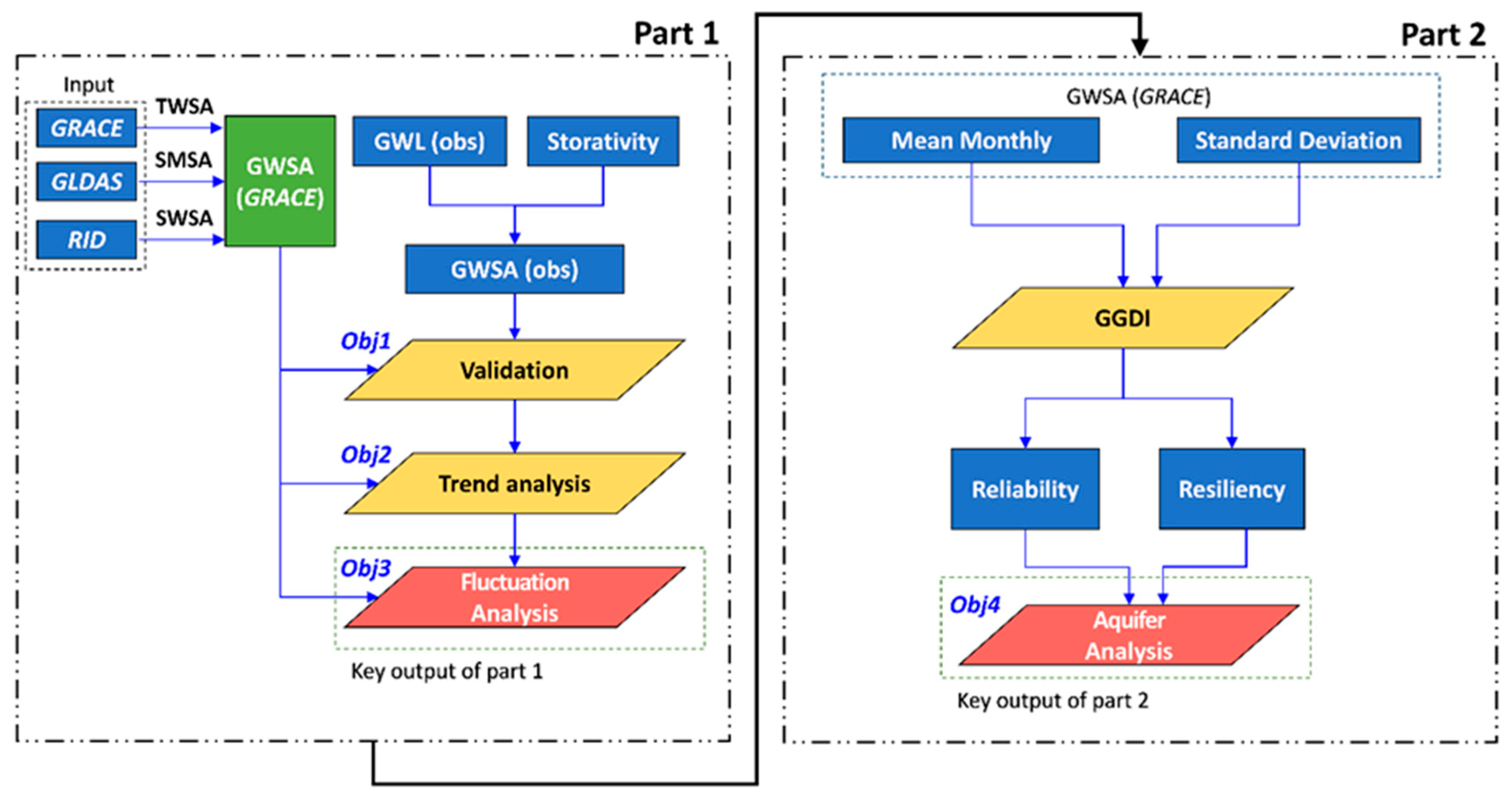
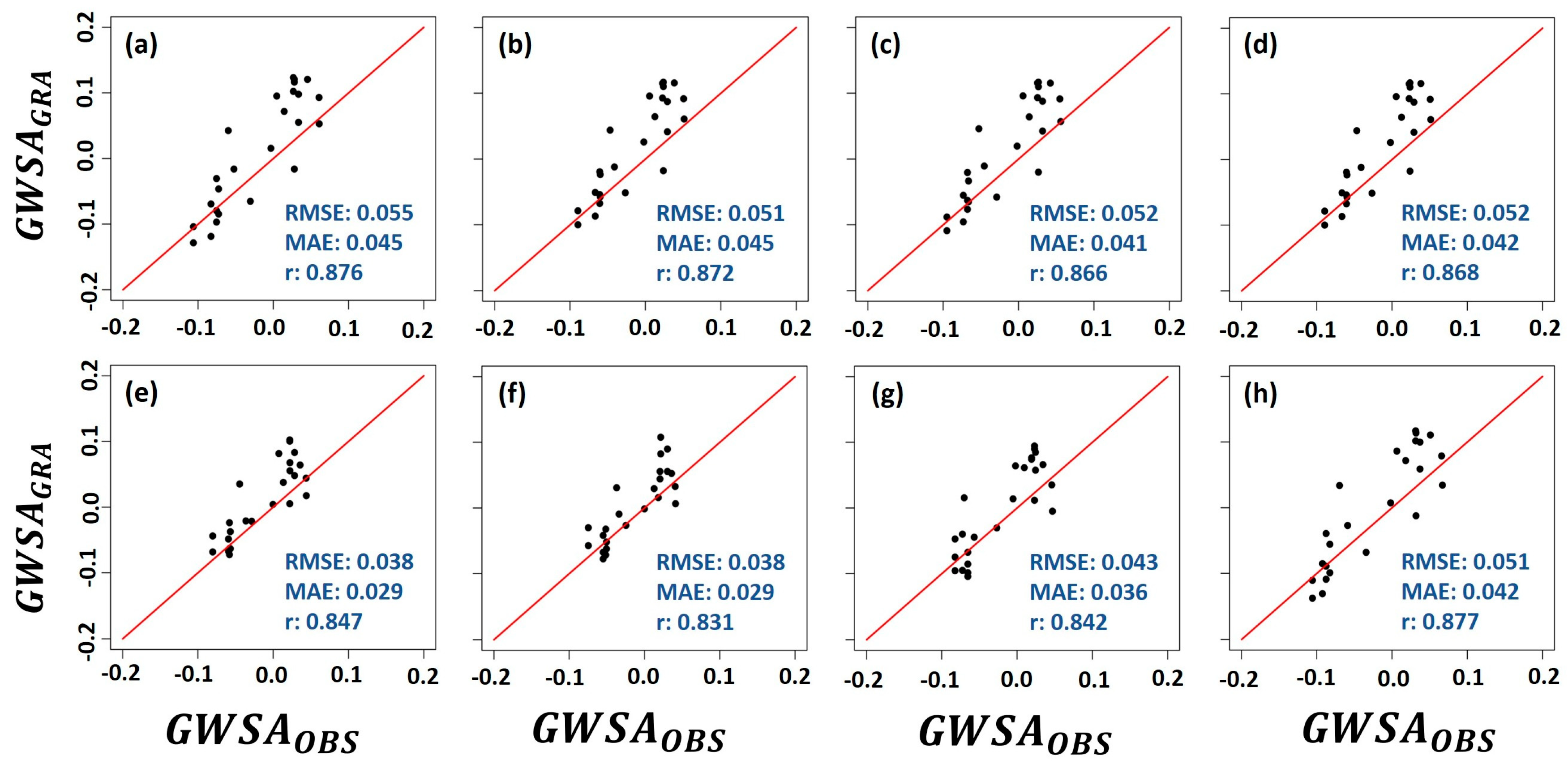
Validate the accuracy of GRACE-derived GWSA (i.e., ${GWSA}_{GRA}$) against in situ data-based GWSA (i.e., ${GWSA}_{obs}$), ensuring the reliability of the datasets before their subsequent application.

(b)

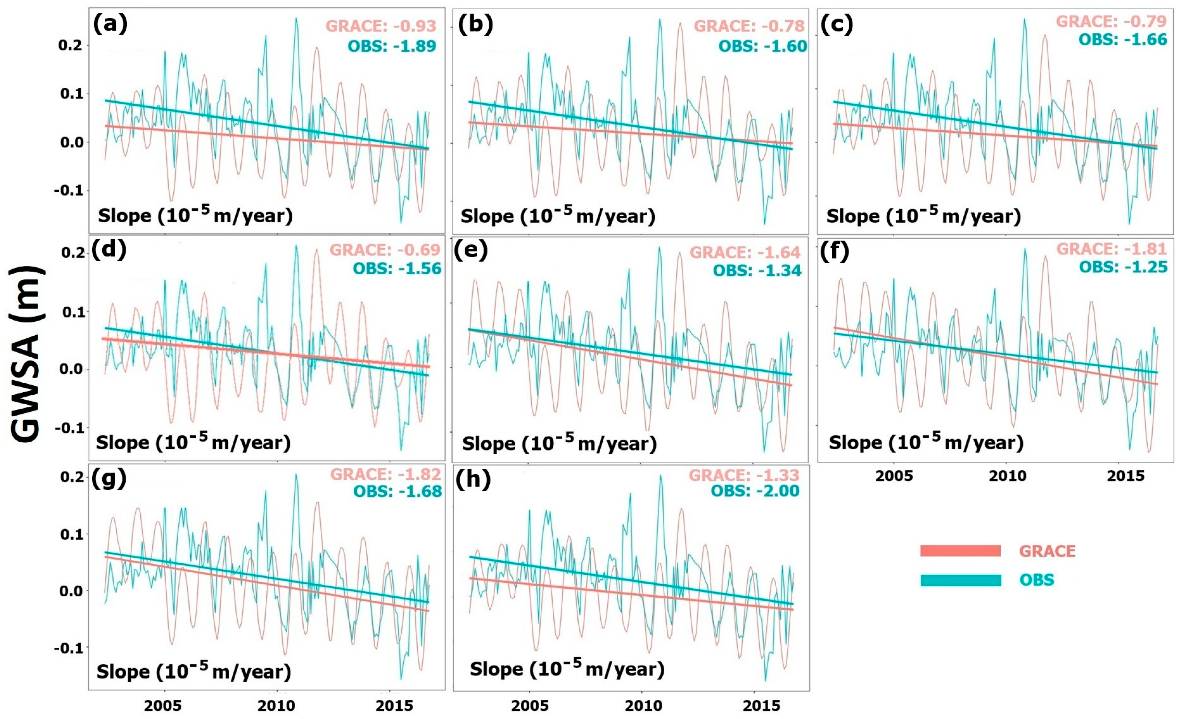
Examine the consistency of temporal trends between ${GWSA}_{GRA}$ and ${GWSA}_{obs}$.

(c)

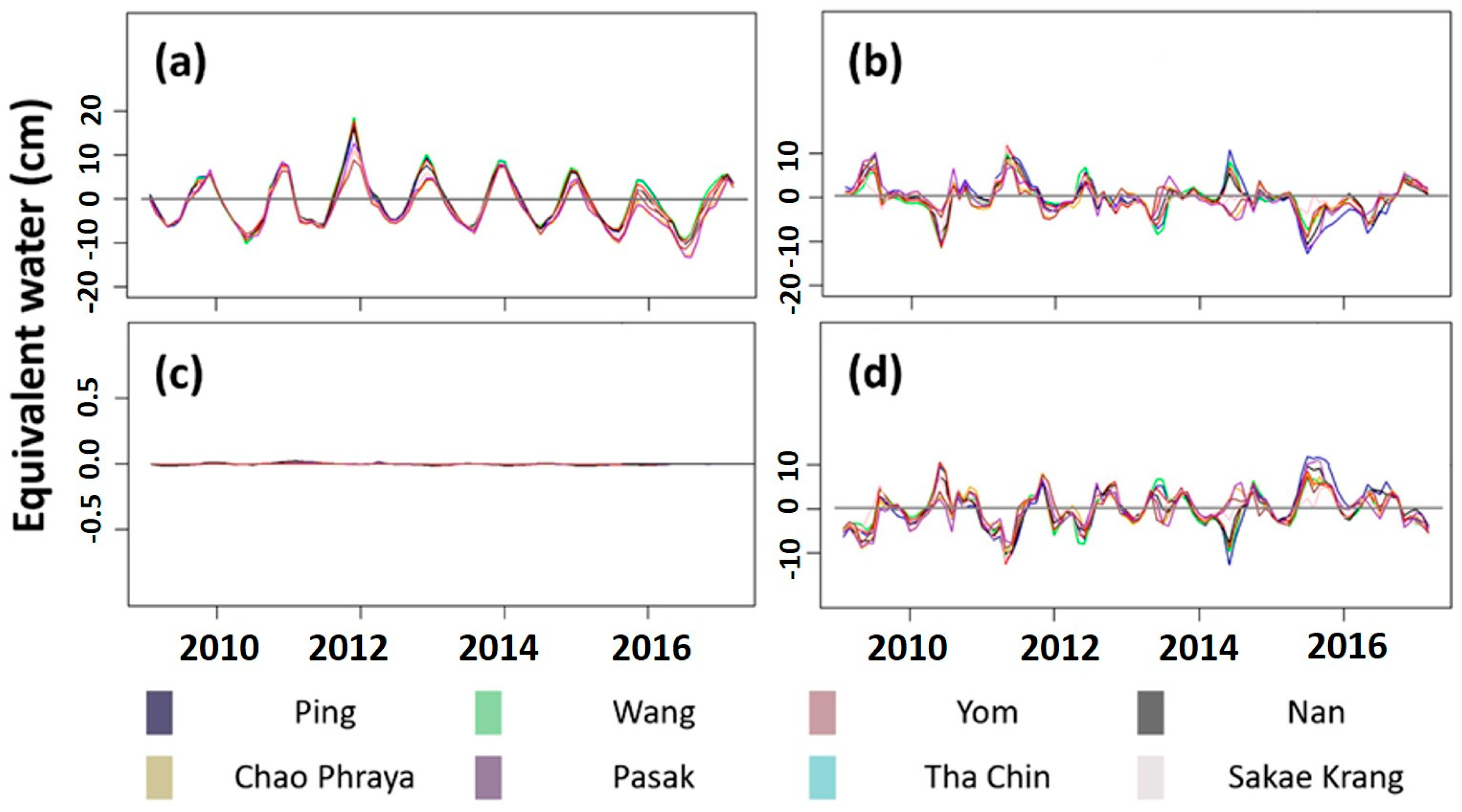
Assess GWSA fluctuations.

(d)

Conduct a thorough analysis of aquifer resilience and reliability using the GGDI.

By accomplishing these goals, our study advances knowledge of groundwater dynamics in the CPR basin and shows how to use current satellite-based techniques in a flexible and useful way. The study’s strength is not a new algorithm, but rather the way it combines established hydrological metrics (e.g., GGDI, reliability, and resilience indices) with remote sensing data (GRACE and GLDAS) to create a cohesive framework for large-scale groundwater assessment. This methodology offers stakeholders a useful tool to support well-informed, data-driven decisions in groundwater resource management because it is scalable and transferable across various hydrological settings. In order to address the ongoing difficulties of groundwater monitoring and management, especially in areas with limited data, the study highlights the significance of incorporating cutting-edge remote sensing technologies.

2. Data Description

2.1. Study Area

The Chao Phraya River (CPR) basin, illustrated in Figure 1 in the, spans an expansive area of 160,000 km², with agriculture dominating 90% of its landscape. It is home to an estimated 30 million people [24]. The southern part of the basin is a low-lying area with elevations as low as 2.5 m above Mean Sea Level (MSL), making it prone to significant flooding events. The basin experiences a tropical monsoon climate, with average daily temperatures hovering around 27 °C, occasionally soaring above 40 °C. Annual rainfall averages 150 cm, ranging from 100 to 200 cm across the basin from west to east. Approximately 90% of the rainfall occurs during the monsoon season from May to October, resulting in an average runoff of 25–45 cm in the basin, with 85% of this runoff occurring from July to December [25]. During the dry season (January to June), limited rainfall results in low natural flows. This leads to a periodic transition from surface water to groundwater as the primary water source, depending on water availability and related policies in the basin.

In the CPR basin, there are two types of aquifers: confined and unconfined [26,27]. However, a confined aquifer is further distributed in several aquifers based on their depth [26,28,29,30]. Bangkok, the capital city, is uniquely situated on a tidal zone and marine clay tidal flat. This marine clay, known as Bangkok clay, forms a layer 15–30 m thick beneath the city’s surface. Overlying the basement, unconsolidated and semi-consolidated sediments have a total thickness of 400 m to over 1800 m. The aquifer system in the CPR basin is primarily composed of layers of sand and gravel, interspersed with clay, and includes eight identified aquifers at depths reaching approximately 600 m. The majority of the CPR basin features a confined aquifer [31], while certain areas in the Chiang Mai region contain unconfined aquifers [32]. The topmost aquifer has non-potable water due to high salinity. The subsequent three aquifers (Phra Pradaeng: 100 m, Nakhon Luang: 150 m, and Nonthaburi: 200 m) are commonly used, while deeper wells with high production primarily serve industrial purposes [33]. Excessive groundwater usage for agriculture and industry raises concerns about its sustainability. In the CPR basin’s southern regions, an average groundwater level decline of 10 cm/year between 1996 and 2008 suggests potential over-pumping issues [34]. Moreover, with the increase in population and anthropogenic activities in the CPR catchment, the aquifer becomes more vulnerable and less reliable and resilient [35].

The CPR basin is divided into eight distinct sub-basins: Ping, Wang, Yom, Nan, Chao Phraya (sub-basin), Pasak, Tha Chin, and Sakae Krang, arranged geographically from west to east and north to south as shown in Figure 1. Each sub-basin exhibits unique hydrological characteristics, prompting a detailed analysis.

2.2. Datasets

2.2.1. GRACE

The GRACE twin-satellite mission measures Earth’s gravity field to study terrestrial water storage variations, with data processed by three centers: CSR at the University of Texas, GFZ in Germany, and JPL in California [15,36]. For our research, we used JPL’s GRACE Terrestrial Water Storage Anomaly (TWSA) Level 3 product, release 06 version 4, from April 2002 to March 2017. This product provides mascon solutions with a spatial resolution of 0.5° × 0.5° [37] and includes a gain factor from the Physical Oceanography Distributed Active Archive Center (PODAAC) at JPL. Notably, from 2011, battery management issues led to periodic data collection gaps, resulting in approximately 12% of the data (22 months) being unavailable [35,36,37,38,39]. We addressed these gaps by linear temporally interpolating data from adjacent months as used by past studies [40,41,42].

2.2.2. GLDAS

NASA collaborates with the National Centers for Environmental Prediction (NCEP) and the National Oceanic and Atmospheric Administration (NOAA) to produce the Global Land Data Assimilation System (GLDAS) datasets, which integrate advanced land surface modeling and data assimilation techniques using satellite-based and observed data [19]. We used baseflow data from the GLDAS database from 2009 to 2017 that came from the NOAH10-M and VIC10-M Land Surface Models (LSMs), which both provide monthly data with a resolution of 0.25° × 0.25° [18,43]. Assuming that baseflow is largely maintained by groundwater discharge in the study region, baseflow was used to indirectly validate the GWSA trends even though it was not directly used in Equation (1). Because of its demonstrated ability to replicate baseflow in Southeast Asia, VIC10-M was chosen, and NOAH10-M was added for comparison in order to guarantee model consistency. The most efficient assessment of groundwater storage is achieved by combining GRACE and GLDAS, according to research [44,45].

2.2.3. In Situ Data

We collected daily water storage data from April 2009 to March 2017 from 13 reservoirs and dams, shown in Figure 1, sourced from the RID online portal [46,47]. These data helped estimate surface water storage across the CPR basin. Additionally, we analyzed data from 1600 functional groundwater wells reported by the Department of Groundwater Resources (DGR) [48]. From these, 120 wells were selected based on their data completeness and regularity over 90%. Groundwater wells located in high terrain within the upper sub-basins (Ping, Wang, Yom, and Nan) are included in the calculations. These wells are situated in unconfined aquifers, with storage coefficients varying from 0.1 to 0.3 for unconfined to confined aquifers, respectively. The process of calculating GWSA is consistent across both high terrain and plain areas. Although snow storage can significantly impact groundwater storage in mountainous regions, it is not a factor in the CPR basin, as there is no snow storage in this region. These monthly measurements were utilized to compare groundwater level changes with GRACE satellite data, assessing water level decline rates and estimating Groundwater Drought Indices for aquifer reliability and resilience. Data from 2009 to 2017 were specifically used to align with GRACE data for consistent comparisons as mentioned in

Table 1. Provides a summary of the datasets we employed, detailing variables, product specifications, spatial and temporal resolutions, time periods, and data sources. Details of these datasets are elaborated upon in the subsequent sections.

Data	Product Specification	Spatial/Temporal Resolution	Source
Terrestrial water storage anomaly (TWSA) (cm)	GRACE JPL Mascon Land RL06 V2 (Time Mean: 2004–2009)	0.5° × 0.5°/Monthly	NASA Jet Propulsion Laboratory (JPL) Tellus (2018)
In situ surface water level (SWL) (m MSL)	N/A	Daily	Royal Irrigation Department (RID)
In situ groundwater level (h) (m MSL)	N/A	Monthly	Department of Groundwater Resources (DGR)
Soil moisture storage (SMS) (kg/m2)	GLDAS-2.1 NOAH model	0.25° × 0.25°/Monthly	[43]

. Notably, the average groundwater level was 24 m, ranging from 1.2 to 65 m. Data gaps were interpolated similarly to the method used for GRACE data to maintain data continuity.

3. Methods

3.1. Methodological Flow

To comprehensively understand the groundwater dynamics of the CPR basin, we applied a methodological framework, as illustrated in Figure 2, segmented into two parts. In this study, all water storage components are monthly time series anomalies averaged over the basin and expressed in terms of equivalent water depth (cm) relative to the long-term mean of each respective time series.

The first part of our methodology, as represented on the left-hand side of Figure 2, focuses on the validation, trend analysis, and fluctuation analysis of groundwater storage (GWS) changes. Initially, all collected datasets underwent preprocessing, which included filling missing data and resampling to the desired resolution using bilinear interpolation. For the GRACE datasets, we applied a gain factor and adjusted their resolution to 0.25° × 0.25°. Bilinear interpolation was employed because, as prior research has shown, it is straightforward, effective, and capable of maintaining the smooth spatial properties of gridded satellite data, including GRACE [49,50]. To maintain alignment with TWSA, we transformed Soil Moisture Storage (SMS) and Surface Water Storage (SWS) components into their respective anomalies. The GWS anomalies (GWSA) were then derived by subtracting SMSA and SWSA from TWSA.

For the observed groundwater levels, we converted them to in situ GWS values, leveraging the aquifer system’s storage coefficient specific to each observation well’s location. These values were further transformed into in situ GWSA values. A pivotal aspect of this phase was the validation of in situ GWSA against GRACE-observed GWSA values, setting the stage for a subsequent trend analysis between the two.

The second part of our methodology, as shown on the right-hand side of Figure 2, revolves around the assessment of the aquifer’s resilience and reliability. Drawing insights from the trend and fluctuation analysis of GWSA, we introduced the GRACE Groundwater Drought Index (GGDI) as a metric to evaluate the aquifer’s health in the CPR basin.

The subsequent subsections will provide a detailed breakdown of each of these methodological components, offering a more in-depth perspective on our approach and its implications.

3.2. GRACE-Derived GWSA

The calculation of TWSA, a crucial hydrological component, is performed as follows in Equation (1):

$$TWSA=SMSA+SWSA+SNSA+\mathrm{C}NSA+GWSA$$

(1)

Here, SMSA represents the total soil moisture anomaly, SWSA encompasses anomalies from all surface water elements like lakes and reservoirs, SNSA refers to the snow water storage anomaly, CNSA to the canopy storage anomaly, and GWSA indicates the groundwater storage anomaly.

To generate TWSA from GRACE, we composed a time series by compositing three products: CSR-M, GFZ-SH, and JPL-M. SMSA was derived by subtracting the baseline mean from the GLDAS soil moisture storage data.

We conducted an in-depth analysis of surface water storage (SWS) data, focusing on reservoirs and dams within the region due to their significant storage capacities [51,52]. The SWSA was calculated by measuring deviations from the average annual storage values from 2009 to 2017. The locations of the studied reservoirs and dams are shown in Figure 1.

Snow water storage (SNS) was excluded from our analysis due to its absence in the study area, and canopy water storage (CNS) fluctuations were below GRACE’s detection threshold [53,54]. As a result, GWSA values, denoted as ${GWSA}_{GRA}$, were straightforwardly derived by subtracting SWSA and SMSA values from TWSA.

3.3. In Situ Data-Derived GWSA

The GWSA, derived from in situ data as ${GWSA}_{obs}$, utilized data from 120 groundwater wells across the eight sub-basins, as shown in Figure 1. The calculation is defined as follows:

$${GWS}_{obs}=\left(h_m-h_i\right)S,$$

(2)

where $h_m$ is the mean groundwater level during the baseline period of 2004–2009, $h_i$ is the level at a specific time, and $S$ is the storage coefficient, ranging from 0 to 0.3, based on the aquifer’s formation [9,55,56,57]. For confined aquifers, S was calculated using the formula $\mathrm{S}=S_s\cdot \mathrm{b}$ where b is the aquifer thickness. For the study area, a representative value of 0.3 was employed.

For processing, monthly ${GWSA}_{obs}$ was calculated by multiplying monthly groundwater levels by each well’s specific storage coefficient (Equation (2)) and then transforming these values using the baseline mean. We employed the inverse distance weighting method to interpolate these values across sub-basin levels, creating continuous raster grids that prioritize closer data points [58,59]. This interpolation and categorization of wells by aquifer depth ensured a consistent distribution of groundwater data across the region.

3.4. Evaluation Metrics

We evaluated the performance of ${GWSA}_{GRA}$ against ${GWSA}_{obs}$ using key statistical metrics: Root Mean Square Error (RMSE), Pearson correlation coefficient (r), and Mean Absolute Error (MAE), with the detailed calculations provided in Equations (3) to (5). These metrics were computed for each sub-basin, and the correlation coefficient was specifically calculated between each well and its corresponding GRACE grid value in cases where multiple wells were located within a single GRACE data grid [27]. The equations for these metrics are as follows:

$$RMSE=\sqrt{{\displaystyle \frac{1}{n}}{\sum }_{i=1}^n{\left({GWSA}_{GRA}\right(i)-{GWSA}_{obs}(i\left)\right)}^2},$$

(3)

$$r={\displaystyle \frac{\sum \left({GWSA}_{GRA}-\overline{{GWSA}_{GRA}}\right)\left({GWSA}_{obs}-\overline{{GWSA}_{obs}}\right)}{\sqrt{\sum {\left({GWSA}_{GRA}-\overline{{GWSA}_{GRA}}\right)}^2}\sqrt{\sum \left({GWSA}_{obs}-{GWSA}_{obs}\right)}}},$$

(4)

$$MAE={\displaystyle \frac{1}{n}}{\sum }_{i=1}^n\left|{GWSA}_{GRA}\left(i\right)-{GWSA}_{obs}\left(i\right)\right|,$$

(5)

where $\overline{{GWSA}_{GRA}}$ and $\overline{{GWSA}_{obs}}$ are the mean values of ${GWSA}_{GRA}$ and ${GWSA}_{obs}$, respectively. $n$ is the total number of data points considered for evaluation.

3.5. GRACE Groundwater Drought Index (GGDI)

In order to evaluate groundwater drought conditions, we employed the GGDI as a dimensionless indicator in our study. We first used the following formula to calculate the monthly climatology $C_i$ for each calendar month i (where i = 1, 2, …, 12) in order to normalize and account for the seasonal variations in groundwater storage as mentioned in Equation (6),

$$C_i={\displaystyle \frac{1}{n_i}}{\sum }_{j=1}^{n_i}GWS{A}_{i,j},$$

(6)

where

• $C_i$ is the average groundwater storage anomaly for month i;
• $GWS{A}_{i,j}$ is the groundwater storage anomaly for the j^th year in month i;
• n_i is the number of years with available GRACE data for month iii (in our case, 15 years from 2002 to 2017).

Standardized anomalies, the foundation of GGDI, are then calculated using this monthly climatology. GGDI provides a consistent and seasonally adjusted depiction of drought severity by eliminating the climatological mean and capturing variations from normal groundwater conditions [60].

To derive the GGDI, we centered and normalized GWSA values by adjusting them based on their mean and scaling by their standard deviation. This standardization quantifies the normalized net deviation in groundwater storage volume. The classification criteria for GGDI, as suggested by [61]. GGDI is intrinsically correlated since it is a standardized (Z-score) version of GWSA. Groundwater drought is indicated by persistently negative GGDI values, summarized in

Table 2. Drought classification based on the GRACE Groundwater Drought Index (GGDI) values.

Grade	Classification	GGDI
I	No Drought	−0.5 < GGDI
II	Mild Drought	−1.0 < GGDI ≤ −0.5
III	Moderate Drought	−1.5 < GGDI ≤ −1.0
IV	Severe Drought	−2 < GGDI ≤ −1.5
V	Extreme Drought	GGDI ≤ −2.0

. GGDI values were used in this study to categorize groundwater conditions: an unsatisfactory state (GGDI < 0) represents drought or scarcity conditions, while a satisfactory state (GGDI ≥ 0) indicates groundwater availability at or above the mean historical level.

3.6. Aquifer Reliability and Resilience

Aquifer reliability measures the probability that an aquifer system remains in a satisfactory state [62]. When applied to GGDI, reliability quantifies how often GGDI values meet or exceed a set threshold (e.g., GGDI ≥ 0), and is expressed as follows in Equation (7):

$$\alpha =\underset{n\to \mathrm{\infty }}{\mathit{lim}}{\displaystyle \frac{1}{n}}{\sum }_{t=1}^n{X}_t,$$

(7)

where X_t = 1 if GGDI at time t indicates a satisfactory state (e.g., GGDI ≥ 0), and X_t = 0 otherwise. Aquifer resilience quantifies how quickly a system returns to a satisfactory state after a drought. It is defined by the transition probability. It is measured by the probability $\gamma$ of transitioning from an unsatisfactory (failure) to a satisfactory state, calculated over time. This probability, $\rho$, involves assessing changes in GGDI values from negative to positive and is computed as follows in Equation (8):

$$\rho =\underset{n\to \mathrm{\infty }}{\mathit{lim}}{\displaystyle \frac{1}{n}}{\sum }_{t=1}^n{W}_t,$$

(8)

where W_t = 1 only when there is a transition from an unsatisfactory to a satisfactory state, i.e., when X_t−1 = 0 and X_t = 1, and W_t = 0 otherwise. Simply put, the probability that the system will remain in an unsatisfactory state $\mathrm{P}\left({\mathrm{X}}_t=0\right)$, is simply $1-\alpha$, where $\alpha$ stands for reliability, or the long-term average of satisfactory conditions. Consequently, resilience γ can be computed as follows in Equation (9):

$$\gamma ={\displaystyle \frac{\rho }{1-\alpha }}.$$

(9)

This demonstrates how fast the system can bounce back from an unsatisfactory state, demonstrating its capacity to return to normal and preserve stability. It is noted that Equation (9) provides a probabilistic estimate of resilience based on binary state transitions, without assuming physically linear groundwater recovery. While this method captures the frequency of recovery events, it does not explicitly account for non-linear behaviors such as hysteresis. Future studies may incorporate lag-based or memory-informed models to better represent such dynamics.

4. Results

Our analysis begins by validating GRACE-derived GWSA (i.e., ${GWSA}_{GRA}$) against in situ data-based GWSA (i.e., ${GWSA}_{obs}$) to confirm the robustness of our data. This critical step ensures the accuracy of the method for wider applications. We then conduct a trend analysis to chart changes in groundwater storage, key to sustainable water resource management. The study examines spatiotemporal variations in groundwater across the sub-basins within the CPR basin, revealing the impact of regional factors. We discuss uncertainties in data resolution and measurement errors and their implications for applying these methods elsewhere. The section closes by considering the aquifer system of the CPR basin, its vulnerability, and the additional information required for extending our approach to other basins. Subsequent subsections provide further details, enhancing our understanding of groundwater dynamics for sustainable management.

4.1. Validation of GRACE-Derived GWSA

In this subsection, our evaluation of ${GWSA}_{GRA}$ against ${GWSA}_{obs}$ spans across the eight distinct sub-basins (Figure 3)—Ping, Wang, Yom, Nan, Chao Phraya, Pasak, Tha Chin, and Sakae Krang. This rigorous assessment lays the groundwork for the broader results and discussions to follow. The period from 2015 to 2017 was specifically selected for this analysis due to the enhanced quality and consistency of the in situ data available during these years.

The scatter plots depicted in Figure 1 reveal a strong correspondence with the 1:1 line, signifying a robust correlation between ${GWSA}_{GRA}$ and ${GWSA}_{obs}$, with Pearson correlation coefficients ($r$) ranging from 0.83 to 0.87 across the sub-basins. Strong and consistent agreement between GRACE-based and observed GWSA values was indicated by all correlation coefficients shown in Figure 3 being statistically significant (p < 0.001). The precision of the GRACE data for groundwater monitoring within these areas is further emphasized by Root Mean Square Error (RMSE) values between 0.036 and 0.045 cm and Mean Absolute Error (MAE) ranging from 0.029 to 0.045.

These results resonate with the findings of previous research, underlining the effectiveness of GRACE data for estimating groundwater storage. For instance, [63] found a correlation of 0.58 across the High Plains Aquifer using 2700 monitoring wells, while [64] reported a strong correlation (r > 0.70) employing over 15,000 wells in Bangladesh. High correlations were also documented by [34] in four Indian basins, and similar validation was provided by [63]. These studies collectively highlight the utility of GRACE as a dependable resource for groundwater assessment in diverse geographical settings.

4.2. Trend of GWSA

Understanding groundwater storage dynamics is critical for sustainable water resource management. To this end, we performed a trend analysis across the sub-basins, employing linear regression to examine the time series of ${GWSA}_{OBS}$ and ${GWSA}_{GRA}$ from 2002 to 2017. This analysis provides a comparative perspective on the changes in groundwater storage across various sub-basins.

Comparative trend analysis in Figure 4 highlights a consistent decline in GWSA across all sub-basins, with considerable variations in the rate of change among them. Notably, the trend discrepancies observed for years, such as 2006 and 2014, suggest external influences on groundwater levels, potentially linked to changes in groundwater management policies in Thailand during these periods [34]. A more detailed examination uncovers that the northern sub-basins (Ping, Wang, Yom, and Nan) show more marked declines in observed data, whereas the southern sub-basins, except for Sakae Krang, indicate steeper declines in GRACE data. These variations in trends across sub-basins highlight the influence of localized factors such as policy changes, groundwater abstraction rates, and recharge conditions. Such differences are crucial for understanding the broader application of the methodology to other basins that may exhibit similar heterogeneities.

However, it is imperative to consider the uncertainties in these results, particularly where data suitability is less robust, as seen in the Sakae Krang basin. The intermittent availability of data for the Nan and Pasak basins and the alignment of observed and GRACE data in the Ping and Yom basins around 2015 further emphasize the need for caution in interpreting these trends. When applying this approach to other basins, a comprehensive understanding of local conditions and the availability of consistent, high-quality data are essential. These factors, including the frequency of data collection and the socio-economic practices influencing groundwater use, play a significant role in the accurate assessment and application of the GRACE data to monitor groundwater trends in diverse hydrological settings.

The observed similarities in the time series for the Ping, Wang, Yom, and Nan basins can be attributed to the geographical and hydrological characteristics of these sub-basins, which share similar climatic conditions and land-use practices. However, the discrepancies between the time series of ${GWSA}_{OBS}$ and ${GWSA}_{GRA}$ may be due to differences in data resolution and the interpolation methods employed. These methodological choices aimed to enhance the reliability of the data, but inherent limitations in spatial coverage and temporal resolution could lead to variations in trend analysis.

4.3. Fluctuation of GWSA

This section presents a detailed examination of GWSA fluctuation. Figure 5 provides a comprehensive visual representation, illustrating the time series for anomalies of terrestrial water storage, soil moisture, surface water storage, and groundwater storage across the eight sub-basins, spanning from April 2009 to March 2017.

Figure 5a shows that TWSA varied between −18 cm and +20 cm, with a notable peak in 2011 corresponding to a significant flood event and a drop in late 2015 indicating drought conditions. The observed similarities in the TWSA time series for the eight sub-basins can be attributed to the integrated nature of terrestrial water storage, which encompasses soil moisture, surface water, and groundwater components. These components are influenced by regional climatic conditions, which tend to be consistent across the sub-basins, leading to analogous TWSA patterns. SMSA in Figure 5b fluctuated within ±10 cm, reflecting changes crucial for understanding groundwater recharge dynamics.

SWSA dynamics, depicted in Figure 5c, showed minimal variation, contributing only 2-3% to the total TWSA and displaying a slight declining trend of −0.04 ± 0.003 cm/year. The relative stability in the SWSA time series is due to the regulated nature of the reservoirs and dams within the CPR basin. These reservoirs are managed to maintain specific water levels, resulting in minimal temporal variation. Unlike previous studies that analyzed SWSA at a grid scale [65], our sub-basin-level assessment resulted in less pronounced fluctuations, smoothing out local variations. Given the larger area of the sub-basins, local variations in storage are averaged out, leading to this stability.

Finally, Figure 5d presents the GWSA oscillating between −12 cm and +12 cm. Unlike the predictable cycle of SMSA, GWSA showed complex variability, hinting at influences beyond climatic conditions, such as anthropogenic activities or other geophysical processes, impacting groundwater dynamics.

These results reveal the diverse hydrological responses among the sub-basins, with variability in GWSA suggesting distinct groundwater recharge and usage patterns. The minimal SWSA fluctuations contrast with the pronounced TWSA and GWSA changes, emphasizing the need for basin-specific water management strategies. Recognizing these disparities is key to understanding the potential for similar satellite-based methodologies in other basins. The presented uncertainties, particularly in GWSA due to anthropogenic influences, highlight the necessity for localized groundwater use data to ensure accurate applications of this approach in different hydrogeological contexts.

The severe drought of 2015 (GGDI < 2.0) is consistent with increased groundwater abstraction documented in 2014–2016 [31,66,67], especially in the central CPR basin, where decreased surface water availability prompted increased agricultural pumping [31,65,68]. Sharp drops in groundwater levels in in situ well data (see Figure 4 and Figure 5d) further support this, indicating a significant human influence on the severity of the drought.

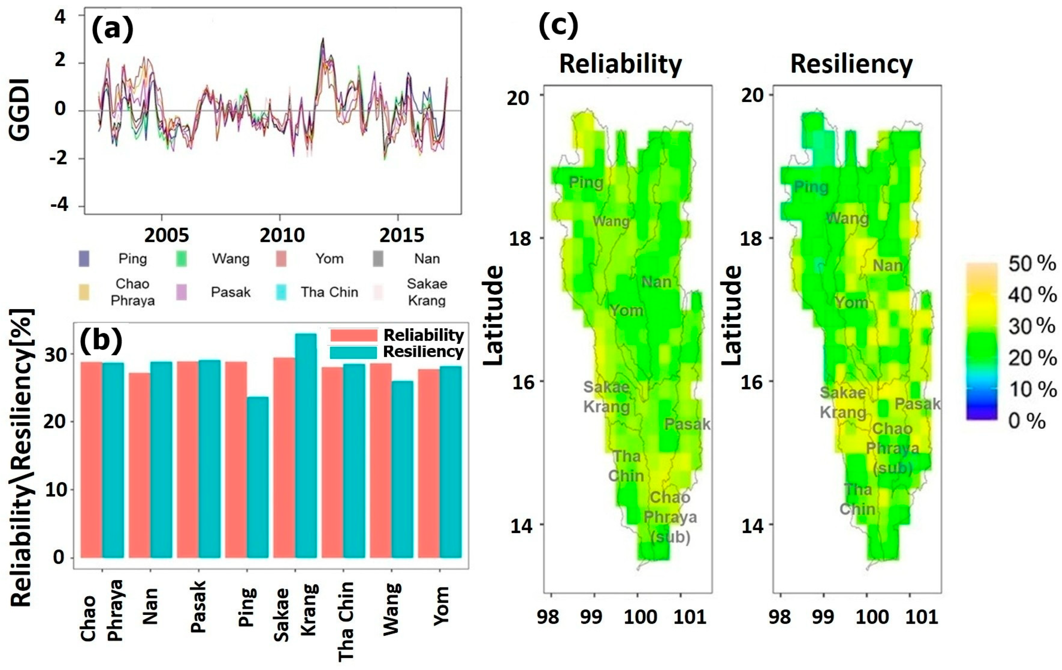
4.4. Aquifer Reliability and Resiliency

This section analyzes the CPR basin, a vital regional water source increasingly vulnerable to environmental stressors. Utilizing the GGDI from 2002 to 2017, we assess the aquifer reliability and resilience, highlighting its current state and challenges.

The GGDI time series, shown in Figure 6a, indicates an increased frequency of droughts over the 15-year period, underlining the vulnerability of the basin groundwater system. The most severe drought occurred in mid-2015, with GGDI values below −2.0, consistent with the findings of [69]. Additionally, severe drought conditions occurred multiple times, as indicated in Table 2, affecting all eight sub-basins and emphasizing the need for proactive drought management strategies. Interestingly, the GGDI also captured significant flooding events, such as the devastating 2011 floods, which are detailed by [70]. These floods, caused by extended periods of heavy rainfall, led to a temporary increase in terrestrial water storage and provided short-term aquifer recharge.

Towards the conclusion of this study, we focus on aquifer reliability and resilience, as depicted in Figure 6b. Alarmingly, most sub-basins show reliability and resilience rates below 30%, except Sakae Krang, which exhibits resilience over 30%. The resilience of the Ping sub-basin is particularly low, under 25%. Figure 6c presents a spatial view of these metrics across the basin, highlighting the geographical variations in aquifer performance.

The limited resilience of the CPR basin to hydrological stress, particularly evident in the Ping sub-basin, highlights the necessity for a robust monitoring and management framework. Such a system is essential to adapt to and mitigate the impacts of regional changes on groundwater systems, ensuring sustainable resource use amid evolving environmental challenges. Tailoring this approach to account for local variations is vital for its application in diverse settings, where region-specific data can address uncertainties and refine the methodology for broader use.

5. Limitations and Future Work

Our study on groundwater dynamics in the CPR basin using GRACE/GRACE-FO satellite gravimetry data revealed several inherent limitations. The spatial resolution of these data, dictated by factors like inter-satellite distance and satellite altitude, affects the granularity of mass change detection on Earth’s surface [71]. While higher resolution can discern small-scale changes due to localized activities, lower resolution might overlook such variations. This limitation is critical as it influences the accuracy of the groundwater storage (GWS) estimates and, consequently, the GGDI. Future satellite missions with improved configurations could enhance data resolution and accuracy [72].

Recent advancements in downscaling techniques have shown promise in improving data resolution and reducing cell dimensions, which could be applied to enhance the granularity of GRACE data [71]. Additionally, the integration of quantitative and qualitative changes in groundwater, such as using detailed groundwater monitoring data for validation, can improve the accuracy of GRACE calculations [10].

Another challenge is the non-uniqueness of mass inversion in GRACE data, which complicates extracting precise changes in mass from observed gravity changes [73]. This issue could limit broader application of GRACE data in evaluating GGDI. Additionally, integrating cutting-edge technologies like artificial intelligence and machine learning could refine data processing and interpretation [74]. Several strategies can be used to lessen the non-uniqueness of mass inversion in GRACE data. The inversion process is constrained, and ambiguity is decreased by incorporating auxiliary datasets like land surface models, in situ groundwater observations, and GLDAS outputs [10,20]. Furthermore, it has been demonstrated that using data assimilation frameworks, mascon solutions, and regularization techniques can improve spatial resolution and lower errors in mass change estimates [75,76]. When combined, these techniques enhance the interpretation of GGDI derived from GRACE.

Innovative methods have also been developed to fill the gap between GRACE and GRACE-FO satellites, ensuring continuity and consistency in the data [36]. Applying these methods could address some of the limitations posed by the temporal gaps in our study.

Our use of GRACE data pre-2018 and the limited availability of in situ data posed further constraints, as integrating newer GRACE-FO data from post-2018 could affect the consistency and credibility of our findings. Furthermore, biased trend interpretations could result from the unequal distribution of observation wells among sub-basins, especially the small number of wells in southern areas like Sakae Krang. Localized variations in groundwater may not be sufficiently recorded as a result of this lack of data. The low sample size made a formal cross-validation impractical, but future research should focus on boosting monitoring density in underrepresented areas to improve the statistical stability and spatial representativeness of basin-scale evaluations.

Despite validating remote sensing-based estimates with data from 120 groundwater wells, the study would benefit from denser, long-term observational networks and more comprehensive storage coefficient data to improve groundwater level to storage volume conversions. Exploring various GRACE dataset versions from different processing centers might also identify the most appropriate data for our study area. Although the storage coefficient is not required for GRACE-based GWSA estimation, it plays a crucial role in deriving in situ GWS estimates from groundwater level data. In this study, a representative range of (S) values was assumed based on previous studies; however, the spatial variability of S across the basin was not explicitly accounted for. This simplification introduces uncertainty in the comparison between in situ and GRACE-derived GWSA. Future work could incorporate spatially distributed S values and sensitivity analyses to better capture local aquifer characteristics. To more accurately depict aquifer heterogeneity and lower uncertainty, future research could use spatially distributed S values obtained from hydrogeological surveys, field measurements, or simulation-based techniques like Monte Carlo analysis. Additionally, while inverse distance weighting (IDW) interpolation was applied for mapping in situ groundwater levels, this method assumes spatial homogeneity and may not fully capture the spatial heterogeneity inherent to large and geologically complex aquifer systems. Future studies could benefit from using more advanced geostatistical methods, such as kriging, to better account for spatial variability.

Although the uncertainties resulting from interpolating in situ observations, processing GRACE data, and correcting the GLDAS model are acknowledged in this study, their full impact on resilience and reliability metrics was not fully quantified. Although these uncertainties are unlikely to change the overall trends and interpretations, they may have an impact on the absolute values. To better contextualize the challenges facing the CPR basin, future research could include uncertainty propagation analysis and comparison with other global basins.

The GGDI classification thresholds used in this study were adopted from prior groundwater resilience studies to enable broad comparability. However, these thresholds were not empirically calibrated to the specific conditions of the CPR basin. This introduces uncertainty, as regional hydrogeological variability may influence groundwater system responses. Future work could refine these thresholds based on local in situ observations or statistical distribution analyses tailored to regional characteristics. The resilience metric applied here assumes linear recovery dynamics, implying a proportional response to stress release. In reality, groundwater systems often exhibit non-linear recovery behaviors, particularly following prolonged droughts or under heterogeneous aquifer conditions. Delayed recharge, soil moisture deficits, and storage thresholds can all lead to asymmetric or hysteretic recovery paths. Future research could incorporate non-linear resilience frameworks to better characterize groundwater system behavior under extreme or persistent stresses.

The validation process inherently faces challenges due to the spatial scale mismatch between GRACE-derived GWSA (~0.5° resolution) and point-based in situ well observations. This discrepancy may lead to aggregation bias, particularly in hydrogeologically diverse regions where groundwater variability occurs at finer spatial scales. While the comparison provides valuable insights at a broad scale, localized discrepancies should be interpreted cautiously. Future work could utilize downscaling methods, higher-resolution satellite products (e.g., GRACE-FO mascons), or spatial averaging of in situ data to reduce the impact of this scale mismatch on validation reliability.

Furthermore, the derived drought metrics may be impacted by the use of bilinear interpolation to fill in the approximately 12% of missing GRACE data that may not fully preserve seasonal fluctuations. Future research should examine alternate techniques like Kalman filtering or kriging to improve temporal fidelity, even though bilinear interpolation is frequently used due to its ease of use and spatial smoothness. Furthermore, the absolute values of the resilience and reliability metrics may be impacted by the aggregation bias resulting from the spatial resolution discrepancy between GRACE (~0.5°) and point-scale well data. It is advised that future research quantify these effects using downscaling methods or sensitivity analyses. As we proceed, addressing these limitations and embracing emerging technologies will be pivotal for refining groundwater evaluation techniques and promoting the sustainable management of water resources. This advancement is not only crucial for the CPR basin but also serves as a benchmark for extending our methodology to other regions, which will necessitate accounting for local hydrological conditions and data-specific challenges to ensure successful applications.

6. Conclusions

Our study offers an encompassing examination of groundwater dynamics, deploying GRACE terrestrial water storage data along with a suite of hydrological datasets to analyze the aquifer system of the Chao Phraya River basin. Our approach, highlighted by the GRACE drought index, enables the exploration of groundwater patterns that are broadly applicable to similar basins. Our findings aligned with our four research objectives as follows:

• Validation of GRACE-derived GWSA: Our analysis demonstrated a strong correlation (over 0.82) between remote sensing data and in situ observations, validating the use of GRACE and GLDAS for monitoring groundwater dynamics across the basin’s eight sub-basins.
• Trend Consistency: We noted a significant declining trend in groundwater storage, highlighting the urgent need for policy measures such as reducing water demand, promoting less water-intensive agriculture, minimizing groundwater dependence, and enhancing groundwater recharge efforts.
• Assessment of Fluctuations: The analysis captured the impact of hydroclimatic extremes on the basin, particularly during the major flood of 2011 and the drought of 2015, revealing multiyear phases of depletion and recovery from 2002 to 2017.
• Analysis of Aquifer Resilience and Reliability: Using the GRACE Groundwater Drought Index, we found alarming resilience and reliability scores, with most sub-basins exhibiting values below 30%. This highlights the vulnerability of the region’s groundwater systems to hydrological stress.
• Future Prospects Using High-Resolution Information: To increase the resolution and applicability of the current model, future studies should make use of higher-resolution datasets. Among these are high-resolution remote sensing tools (e.g., Sentinel, SMAP) and hydrogeophysical exploration techniques for subsurface characterization [77]. Regionally calibrated groundwater level data and socioeconomic water use data. The integration of these datasets will reduce uncertainty, facilitate the estimation of aquifer properties, and more accurately account for human impacts on groundwater systems [78].

These key findings underline the importance of robust groundwater management practices. The demonstrated methodology using GRACE and GLDAS data offers a replicable framework that can be applied globally, providing substantial benefits for sustainable water resource management. Future studies should focus on integrating higher-resolution datasets and expanding the observational network to further refine groundwater assessment techniques.

References

1. Griebler, C.; Avramov, M. Groundwater Ecosystem Services: A Review. Freshw. Sci. 2015, 34, 355–367. [Google Scholar] [CrossRef]
2. Sokneth, L.; Mohanasundaram, S.; Shrestha, S.; Babel, M.S.; Virdis, S.G.P. Evaluating Aquifer Stress and Resilience with GRACE Information at Different Spatial Scales in Cambodia. Hydrogeol. J. 2022, 30, 2359–2377. [Google Scholar] [CrossRef] [PubMed]
3. Zektser, I.S.; Loaiciga, H.A. Groundwater Fluxes in the Global Hydrologic Cycle: Past, Present and Future. J. Hydrol. 1993, 144, 405–427. [Google Scholar] [CrossRef]
4. Goswami, L.; Tejas Namboodiri, M.M.; Vinoth Kumar, R.; Pakshirajan, K.; Pugazhenthi, G. Biodiesel Production Potential of Oleaginous Rhodococcus Opacus Grown on Biomass Gasification Wastewater. Renew. Energy 2017, 105, 400–406. [Google Scholar] [CrossRef]
5. Giordano, M. Global Groundwater? Issues and Solutions. Annu. Rev. Environ. Resour. 2009, 34, 153–178. [Google Scholar] [CrossRef]
6. Sathe, S.S.; Goswami, L.; Mahanta, C. Arsenic Reduction and Mobilization Cycle via Microbial Activities Prevailing in the Holocene Aquifers of Brahmaputra Flood Plain. Groundw. Sustain. Dev. 2021, 13, 100578. [Google Scholar] [CrossRef]
7. Begum, W.; Goswami, L.; Sharma, B.B.; Kushwaha, A. Assessment of Urban River Pollution Using the Water Quality Index and Macro-Invertebrate Community Index. Environ. Dev. Sustain. 2023, 25, 8877–8902. [Google Scholar] [CrossRef]
8. Famiglietti, J.S. The Global Groundwater Crisis. Nat. Clim. Chang. 2014, 4, 945–948. [Google Scholar] [CrossRef]
9. Bhanja, S.N.; Rodell, M.; Li, B.; Saha, D.; Mukherjee, A. Spatio-Temporal Variability of Groundwater Storage in India. J. Hydrol. 2017, 544, 428–437. [Google Scholar] [CrossRef]
10. Scanlon, B.R.; Zhang, Z.; Save, H.; Sun, A.Y.; Müller Schmied, H.; Van Beek, L.P.H.; Wiese, D.N.; Wada, Y.; Long, D.; Reedy, R.C.; et al. Global Models Underestimate Large Decadal Declining and Rising Water Storage Trends Relative to GRACE Satellite Data. Proc. Natl. Acad. Sci. USA 2018, 115, E1080–E1089. [Google Scholar] [CrossRef]
11. Chen, J.; Famigliett, J.S.; Scanlon, B.R.; Rodell, M. Groundwater Storage Changes: Present Status from GRACE Observations. Surv. Geophys. 2016, 37, 397–417. [Google Scholar] [CrossRef]
12. Sharma, Y.; Aggarwal, A.; Singh, J. Development of Flow Duration Curves and Eco-Flow Metrics for the Tawi River Basin—(Jammu, India). Int. J. Adv. Remote Sens. GIS 2019, 8, 3114–3125. [Google Scholar] [CrossRef]
13. Bremard, T. Monitoring Land Subsidence: The Challenges of Producing Knowledge and Groundwater Management Indicators in the Bangkok Metropolitan Region, Thailand. Sustainability 2022, 14, 10593. [Google Scholar] [CrossRef]
14. Thomas, B.F.; Famiglietti, J.S. Identifying Climate-Induced Groundwater Depletion in GRACE Observations. Sci. Rep. 2019, 9, 4124. [Google Scholar] [CrossRef]
15. Tapley, B.D.; Bettadpur, S.; Watkins, M.; Reigber, C. The Gravity Recovery and Climate Experiment: Mission Overview and Early Results: GRACE MISSION OVERVIEW AND EARLY RESULTS. Geophys. Res. Lett. 2004, 31, L09607. [Google Scholar] [CrossRef]
16. Castellazzi, P.; Longuevergne, L.; Martel, R.; Rivera, A.; Brouard, C.; Chaussard, E. Quantitative Mapping of Groundwater Depletion at the Water Management Scale Using a Combined GRACE/InSAR Approach. Remote Sens. Environ. 2018, 205, 408–418. [Google Scholar] [CrossRef]
17. Fatolazadeh, F.; Eshagh, M.; Goïta, K. New Spectro-Spatial Downscaling Approach for Terrestrial and Groundwater Storage Variations Estimated by GRACE Models. J. Hydrol. 2022, 615, 128635. [Google Scholar] [CrossRef]
18. Beaudoing, H.; Rodell, M.; NASA/GSFC/HSL. GLDAS Noah Land Surface Model L4 Monthly 1.0 × 1.0 Degree; Version 2.1. 2020. Available online: https://data.nasa.gov/dataset/gldas-noah-land-surface-model-l4-monthly-1-0-x-1-0-degree-early-product-v2-1-gldas-noah10--e0459 (accessed on 15 January 2022).
19. Rodell, M.; Houser, P.R.; Jambor, U.; Gottschalck, J.; Mitchell, K.; Meng, C.-J.; Arsenault, K.; Cosgrove, B.; Radakovich, J.; Bosilovich, M.; et al. The Global Land Data Assimilation System. Bull. Am. Meteorol. Soc. 2004, 85, 381–394. [Google Scholar] [CrossRef]
20. Wang, S.; Liu, H.; Yu, Y.; Zhao, W.; Yang, Q.; Liu, J. Evaluation of Groundwater Sustainability in the Arid Hexi Corridor of Northwestern China, Using GRACE, GLDAS and Measured Groundwater Data Products. Sci. Total Environ. 2020, 705, 135829. [Google Scholar] [CrossRef]
21. Yan, X.; Zhang, B.; Yao, Y.; Yin, J.; Wang, H.; Ran, Q. Jointly Using the GLDAS 2.2 Model and GRACE to Study the Severe Yangtze Flooding of 2020. J. Hydrol. 2022, 610, 127927. [Google Scholar] [CrossRef]
22. Heydarizad, M.; Pumijumnong, N.; Mansourian, D.; Anbaran, E.D.; Minaei, M. The Deterioration of Groundwater Quality by Seawater Intrusion in the Chao Phraya River Basin, Thailand. Environ. Monit. Assess. 2023, 195, 424. [Google Scholar] [CrossRef] [PubMed]
23. Seeboonruang, U. Wavelet Relationship between Climate Variability and Deep Groundwater Fluctuation in Thailand’s Central Plains. KSCE J. Civ. Eng. 2018, 22, 868–876. [Google Scholar] [CrossRef]
24. UNEP-DHI; IWA. Flood & Drought Management Tools. 2014. Available online: https://www.flooddroughtmonitor.com/knowledgeportal. (accessed on 8 February 2022).
25. Komolafe, A.A.; Herath, S.; Avtar, R. Establishment of Detailed Loss Functions for the Urban Flood Risk Assessment in Chao Phraya River Basin, Thailand. Geomat. Nat. Hazards Risk 2019, 10, 633–650. [Google Scholar] [CrossRef]
26. Taweesin, K.; Seeboonruang, U.; Saraphirom, P. The Influence of Climate Variability Effects on Groundwater Time Series in the Lower Central Plains of Thailand. Water 2018, 10, 290. [Google Scholar] [CrossRef]
27. Sharma, Y.K.; Kim, S.; Tayerani Charmchi, A.S.; Kang, D.; Batelaan, O. Strategic Imputation of Groundwater Data Using Machine Learning: Insights from Diverse Aquifers in the Chao-Phraya River Basin. Groundw. Sustain. Dev. 2024, 28, 101394. [Google Scholar] [CrossRef]
28. Kamdee, K.; Corcho Alvarado, J.A.; Yongprawat, M.; Occarach, O.; Hunyek, V.; Wongsit, A.; Saengkorakot, C.; Chanruang, P.; Polee, C.; Uapoonphol, N.; et al. Using 81Kr and Isotopic Tracers to Characterise Old Groundwater in the Bangkok Metropolitan and Vicinity Areas. Isotopes Environ. Health Stud. 2023, 59, 426–453. [Google Scholar] [CrossRef]
29. Lorphensri, O.; Nettasana, T.; Ladawadee, A. Groundwater Environment in Bangkok and the Surrounding Vicinity, Thailand. In Groundwater Environment in Asian Cities; Elsevier: Amsterdam, The Netherlands, 2016; pp. 229–262. ISBN 978-0-12-803166-7. [Google Scholar]
30. Wang, Y.; Chen, G.; Yu, H.; Xu, X.; Liu, W.; Fu, T.; Su, Q.; Zou, Y.; Kornkanitnan, N.; Shi, X. Distribution of 222Rn in Seawater Intrusion Area and Its Implications on Tracing Submarine Groundwater Discharge on the Upper Gulf of Thailand. Lithosphere 2022, 2022, 2039170. [Google Scholar] [CrossRef]
31. Tanachaichoksirikun, P. Groundwater vulnerability of Thailand’s lower Chao Phraya Basin. Int. J. GEOMATE 2020, 18, 88–96. [Google Scholar] [CrossRef]
32. Taweelarp, S.; Khebchareon, M.; Saenton, S. Evaluation of Groundwater Potential and Safe Yield of Heterogeneous Unconsolidated Aquifers in Chiang Mai Basin, Northern Thailand. Water 2021, 13, 558. [Google Scholar] [CrossRef]
33. Buapeng, S.; Wattayakorn, G. Groundwater Situation in Bangkok and Its Vicinity. In Proceedings of the HydrroChange 2008 in KYOTO: Hydrological Changes and Management from Headwater to the Ocean, Kyoto, Japan, 1–3 October 2008. [Google Scholar] [CrossRef]
34. World Bank. Thailand Environment Monitor Integrated Water Resource Management: A Way Forward; World Bank: Washington, DC, USA, 2011. [Google Scholar]
35. Shakti, P.C.; Miyamoto, M.; Misumi, R.; Nakamura, Y.; Sriariyawat, A.; Visessri, S.; Kakinuma, D. Assessing Flood Risk of the Chao Phraya River Basin Based on Statistical Rainfall Analysis. J. Disaster Res. 2020, 15, 1025–1039. [Google Scholar] [CrossRef]
36. Landerer, F.W.; Flechtner, F.M.; Save, H.; Webb, F.H.; Bandikova, T.; Bertiger, W.I.; Bettadpur, S.V.; Byun, S.H.; Dahle, C.; Dobslaw, H.; et al. Extending the Global Mass Change Data Record: GRACE Follow-On Instrument and Science Data Performance. Geophys. Res. Lett. 2020, 47, e2020GL088306. [Google Scholar] [CrossRef]
37. NASA Jet Propulsion Laboratory (JPL) Tellus. JPL GRACE Mascon Ocean, Ice, and Hydrology Equivalent Water Height Release 06 Coastal Resolution Improvement (CRI) Filtered Version 1.0. 2018. Available online: https://podaac.jpl.nasa.gov/dataset/TELLUS_GRACE_MASCON_CRI_GRID_RL06_V1 (accessed on 15 January 2022).
38. Long, D.; Shen, Y.; Sun, A.; Hong, Y.; Longuevergne, L.; Yang, Y.; Li, B.; Chen, L. Drought and Flood Monitoring for a Large Karst Plateau in Southwest China Using Extended GRACE Data. Remote Sens. Environ. 2014, 155, 145–160. [Google Scholar] [CrossRef]
39. Yin, W.; Hu, L.; Zhang, M.; Wang, J.; Han, S. Statistical Downscaling of GRACE-Derived Groundwater Storage Using ET Data in the North China Plain. J. Geophys. Res. Atmos. 2018, 123, 5973–5987. [Google Scholar] [CrossRef]
40. Hu, Y.; Chao, N.; Yang, Y.; Wang, J.; Yin, W.; Xie, J.; Duan, G.; Zhang, M.; Wan, X.; Li, F.; et al. Integrating GRACE/GRACE Follow-On and Wells Data to Detect Groundwater Storage Recovery at a Small-Scale in Beijing Using Deep Learning. Remote Sens. 2023, 15, 5692. [Google Scholar] [CrossRef]
41. Ali, S.; Ran, J.; Khorrami, B.; Wu, H.; Tariq, A.; Jehanzaib, M.; Khan, M.M.; Faisal, M. Downscaled GRACE/GRACE-FO Observations for Spatial and Temporal Monitoring of Groundwater Storage Variations at the Local Scale Using Machine Learning. Groundw. Sustain. Dev. 2024, 25, 101100. [Google Scholar] [CrossRef]
42. Seo, J.Y.; Lee, S.-I. Predicting Changes in Spatiotemporal Groundwater Storage Through the Integration of Multi-Satellite Data and Deep Learning Models. IEEE Access 2021, 9, 157571–157583. [Google Scholar] [CrossRef]
43. Li, B.; Beaudoing, H.; Rodell, M.; NASA/GSFC/HSL. GLDAS Catchment Land Surface Model L4 Monthly 1.0 × 1.0 Degree Early Product V2.1. 2020. Available online: https://hydro1.gesdisc.eosdis.nasa.gov/data/GLDAS/GLDAS_CLSM10_M.2.1/ (accessed on 15 January 2022).
44. Alghafli, K.; Shi, X.; Sloan, W.; Shamsudduha, M.; Tang, Q.; Sefelnasr, A.; Ebraheem, A.A. Groundwater Recharge Estimation Using In-Situ and GRACE Observations in the Eastern Region of the United Arab Emirates. Sci. Total Environ. 2023, 867, 161489. [Google Scholar] [CrossRef]
45. Sarkar, T.; Kannaujiya, S.; Taloor, A.K.; Champati Ray, P.K.; Chauhan, P. Integrated Study of GRACE Data Derived Interannual Groundwater Storage Variability over Water Stressed Indian Regions. Groundw. Sustain. Dev. 2020, 10, 100376. [Google Scholar] [CrossRef]
46. Tariq, A.; Ali, S.; Basit, I.; Jamil, A.; Farmonov, N.; Khorrami, B.; Khan, M.M.; Sadri, S.; Baloch, M.Y.J.; Islam, F.; et al. Terrestrial and Groundwater Storage Characteristics and Their Quantification in the Chitral (Pakistan) and Kabul (Afghanistan) River Basins Using GRACE/GRACE-FO Satellite Data. Groundw. Sustain. Dev. 2023, 23, 100990. [Google Scholar] [CrossRef]
47. Royal Irrigation Department Reservoir Storage Data. 2017. Available online: https://app.rid.go.th/reservoir/ (accessed on 15 January 2022).
48. Department of Groundwater Resources, Thailand. Waterlevel Data. 2021. Available online: https://www.dgr.go.th/ (accessed on 10 March 2022).
49. Long, D.; Longuevergne, L.; Scanlon, B.R. Uncertainty in Evapotranspiration from Land Surface Modeling, Remote Sensing, and GRACE Satellites. Water Resour. Res. 2014, 50, 1131–1151. [Google Scholar] [CrossRef]
50. Feng, W.; Zhong, M.; Lemoine, J.; Biancale, R.; Hsu, H.; Xia, J. Evaluation of Groundwater Depletion in North China Using the Gravity Recovery and Climate Experiment (GRACE) Data and Ground-based Measurements. Water Resour. Res. 2013, 49, 2110–2118. [Google Scholar] [CrossRef]
51. Sayama, T.; Tatebe, Y.; Iwami, Y.; Tanaka, S. Hydrologic Sensitivity of Flood Runoff and Inundation: 2011 Thailand Floods in the Chao Phraya River Basin. Nat. Hazards Earth Syst. Sci. 2015, 15, 1617–1630. [Google Scholar] [CrossRef]
52. Ndehedehe, C.E.; Adeyeri, O.E.; Onojeghuo, A.O.; Ferreira, V.G.; Kalu, I.; Okwuashi, O. Understanding Global Groundwater-Climate Interactions. Sci. Total Environ. 2023, 904, 166571. [Google Scholar] [CrossRef]
53. Liesch, T.; Ohmer, M. Comparison of GRACE Data and Groundwater Levels for the Assessment of Groundwater Depletion in Jordan. Hydrogeol. J. 2016, 24, 1547–1563. [Google Scholar] [CrossRef]
54. Rodell, M.; Chao, B.F.; Au, A.Y.; Kimball, J.S.; McDonald, K.C. Global Biomass Variation and Its Geodynamic Effects: 1982–98. Earth Interact. 2005, 9, 1–19. [Google Scholar] [CrossRef]
55. Bhanja, S.N.; Zhang, X.; Wang, J. Estimating Long-Term Groundwater Storage and Its Controlling Factors in Alberta, Canada. Hydrol. Earth Syst. Sci. 2018, 22, 6241–6255. [Google Scholar] [CrossRef]
56. Johnson, A.J. Specific Yield: Compilation of Specific Yields for Various Materials; United Sates Government Printing Office: Washington, DC, USA, 1967. [Google Scholar]
57. Todd, D.K. Groundwater Hydrology; Wiley and Sons: Hoboken, NJ, USA, 2005; ISBN 0-471-45254-8. [Google Scholar]
58. Lu, G.Y.; Wong, D.W. An Adaptive Inverse-Distance Weighting Spatial Interpolation Technique. Comput. Geosci. 2008, 34, 1044–1055. [Google Scholar] [CrossRef]
59. Sharma, Y.; Tyagi, A.; Sharma, M.L.; Sharma, P.; Aggarwal, A. Building Vulnerability Assessment Using Artificial Intelligence forLandslide Susceptibility Zone in Champawat District, India. In Proceedings of the EGU General Assembly 2023, Vienna, Austria, 24–28 April 2023. [Google Scholar]
60. Thomas, B.F.; Famiglietti, J.S.; Landerer, F.W.; Wiese, D.N.; Molotch, N.P.; Argus, D.F. GRACE Groundwater Drought Index: Evaluation of California Central Valley Groundwater Drought. Remote Sens. Environ. 2017, 198, 384–392. [Google Scholar] [CrossRef]
61. Wang, F.; Wang, Z.; Yang, H.; Di, D.; Zhao, Y.; Liang, Q. Utilizing GRACE-Based Groundwater Drought Index for Drought Characterization and Teleconnection Factors Analysis in the North China Plain. J. Hydrol. 2020, 585, 124849. [Google Scholar] [CrossRef]
62. Maity, R.; Sharma, A.; Nagesh Kumar, D.; Chanda, K. Characterizing Drought Using the Reliability-Resilience-Vulnerability Concept. J. Hydrol. Eng. 2013, 18, 859–869. [Google Scholar] [CrossRef]
63. Strassberg, G.; Scanlon, B.R.; Rodell, M. Comparison of Seasonal Terrestrial Water Storage Variations from GRACE with Groundwater-Level Measurements from the High Plains Aquifer (USA). Geophys. Res. Lett. 2007, 34, L14402. [Google Scholar] [CrossRef]
64. Shamsudduha, M.; Taylor, R.G.; Longuevergne, L. Monitoring Groundwater Storage Changes in the Highly Seasonal Humid Tropics: Validation of GRACE Measurements in the Bengal Basin: VALIDATING GRACE ΔGWS IN THE HUMID TROPICS. Water Resour. Res. 2012, 48, W02508. [Google Scholar] [CrossRef]
65. Abhishek; Kinouchi, T.; Sayama, T. A Comprehensive Assessment of Water Storage Dynamics and Hydroclimatic Extremes in the Chao Phraya River Basin during 2002–2020. J. Hydrol. 2021, 603, 126868. [Google Scholar] [CrossRef]
66. Bangkok; Long, T.T.; Sucharit, K.; Chokchai, S.; Chi, H.; City, M.; Ward, L.T.; District, T.D. Sustainable groundwater pumping in the upper central plain, Thailand and ANN application for available GW pumping. In Proceedings of the 1st Thailand Groundwater Symposium: Key to Water Security and Sustainability, Bangkok, Thailand, 2–26 August 2022. [Google Scholar] [CrossRef]
67. Yang, S.; Zhao, B.; Yang, D.; Wang, T.; Yang, Y.; Ma, T.; Santisirisomboon, J. Future Changes in Water Resources, Floods and Droughts under the Joint Impact of Climate and Land-Use Changes in the Chao Phraya Basin, Thailand. J. Hydrol. 2023, 620, 129454. [Google Scholar] [CrossRef]
68. Tomkratoke, S.; Kongkulsiri, S.; Narenpitak, P.; Sirisup, S. Drought and Salinity Intrusion in the Lower Chao Phraya River: Variability Analysis and Modeling Mitigation Approaches. EGUsphere 2025. preprint. [Google Scholar] [CrossRef]
69. Khairunnisa, A. Thailand Drought 2015: Climate Change Impacts Real. 2015. Available online: https://www.acccrn.net/blog/thailand-drought-2015-climate-change-impacts-real. (accessed on 7 April 2022).
70. Loc, H.H.; Emadzadeh, A.; Park, E.; Nontikansak, P.; Deo, R.C. The Great 2011 Thailand Flood Disaster Revisited: Could It Have Been Mitigated by Different Dam Operations Based on Better Weather Forecasts? Environ. Res. 2023, 216, 114493. [Google Scholar] [CrossRef] [PubMed]
71. Chen, J.; Cazenave, A.; Dahle, C.; Llovel, W.; Panet, I.; Pfeffer, J.; Moreira, L. Applications and Challenges of GRACE and GRACE Follow-On Satellite Gravimetry. Surv. Geophys. 2022, 43, 305–345. [Google Scholar] [CrossRef]
72. Swenson, S.; Chambers, D.; Wahr, J. Estimating Geocenter Variations from a Combination of GRACE and Ocean Model Output. J. Geophys. Res. Solid Earth 2008, 113, 2007JB005338. [Google Scholar] [CrossRef]
73. Velicogna, I.; Wahr, J. Time-Variable Gravity Observations of Ice Sheet Mass Balance: Precision and Limitations of the GRACE Satellite Data: UNDERSTANDING GRACE ICE MASS ESTIMATES. Geophys. Res. Lett. 2013, 40, 3055–3063. [Google Scholar] [CrossRef]
74. Uz, M.; Atman, K.G.; Akyilmaz, O.; Shum, C.K.; Keleş, M.; Ay, T.; Tandoğdu, B.; Zhang, Y.; Mercan, H. Bridging the Gap between GRACE and GRACE-FO Missions with Deep Learning Aided Water Storage Simulations. Sci. Total Environ. 2022, 830, 154701. [Google Scholar] [CrossRef]
75. Save, H.; Bettadpur, S.; Tapley, B.D. High-resolution CSR GRACE RL05 Mascons. J. Geophys. Res. Solid Earth 2016, 121, 7547–7569. [Google Scholar] [CrossRef]
76. Wiese, D.N.; Landerer, F.W.; Watkins, M.M. Quantifying and Reducing Leakage Errors in the JPL RL05M GRACE Mascon Solution. Water Resour. Res. 2016, 52, 7490–7502. [Google Scholar] [CrossRef]
77. Khan, U.; Faheem, H.; Jiang, Z.; Wajid, M.; Younas, M.; Zhang, B. Integrating a GIS-Based Multi-Influence Factors Model with Hydro-Geophysical Exploration for Groundwater Potential and Hydrogeological Assessment: A Case Study in the Karak Watershed, Northern Pakistan. Water 2021, 13, 1255. [Google Scholar] [CrossRef]
78. Wang, L.; Jiang, Z.; Song, L.; Yu, X.; Yuan, S.; Zhang, B. A Groundwater Level Spatiotemporal Prediction Model Based on Graph Convolutional Networks with a Long Short-Term Memory. J. Hydroinform. 2024, 26, 2962–2979. [Google Scholar] [CrossRef]
Figure 1. Map of the Chao Phraya River (CPR) basin, showing its division into eight sub-basins: Ping (18 wells), Wang (9 wells), Yom (12 wells), Nan (17 wells), Chao Phraya (33 wells), Pasak (10 wells), Tha Chin (19 wells), and Sakae Krang (2 wells). Key features include 120 groundwater wells (denoted by orange dots) and 13 reservoirs (marked with star symbols) used for this study.
Remotesensing 17 01731 g001
Figure 2. Methodological workflow of this study: The workflow is composed of two parts. Part 1 encompasses objectives 1 through 3, focusing on the validation, trend analysis, and assessment of GWSA fluctuations. Part 2 centers on the aquifer assessment, drawing from GGDI-based reliability and resiliency metrics. Here, GWSA: groundwater storage anomaly; TWSA: terrestrial water storage anomaly; SMSA: soil moisture storage anomaly; SWSA: surface water storage anomaly; GGDI: GRACE Groundwater Drought Index.
Remotesensing 17 01731 g002
Figure 3. Validation results of G W S A G R A against G W S A O B S across eight sub-basins: (a) Ping, (b) Wang, (c) Yom, (d) Nan, (e) Chao Phraya, (f) Pasak, (g) Tha Chin, and (h) Sakae Krang. The scatter plots reveal a strong correlation between G W S A G R A and G W S A O B S , with Pearson correlation coefficients (r) ranging from 0.83 to 0.87. The enhanced data quality from 2015 to 2017 ensures reliable validation despite the limited number of groundwater wells and irregular monitoring in the upper Chao Phraya basin.
Remotesensing 17 01731 g003
Figure 4. Comparative trend analysis of G W S A O B S and G W S A G R A across eight sub-basins: (a) Ping, (b) Wang, (c) Yom, (d) Nan, (e) Chao Phraya, (f) Pasak, (g) Tha Chin, and (h) Sakae Krang. The time series from 2002 to 2017 shows the variations in groundwater storage. Similarities among the Ping, Wang, Yom, and Nan basins reflect their shared geographic and hydrological characteristics. Differences between G W S A O B S and G W S A G R A highlight the challenges in data resolution and interpolation methods.
Remotesensing 17 01731 g004
Figure 5. Time series of (a) terrestrial water storage anomaly (TWSA), (b) soil moisture storage anomaly (SMSA), (c) surface water storage anomaly (SWSA), and (d) groundwater storage anomaly (GWSA) across the eight sub-basins.
Remotesensing 17 01731 g005
Figure 6. Evaluation results of the CPR basin’s groundwater system: (a) Time series of GRACE-derived GGDI from 2002 to 2017. (b) Estimation of reliability and resilience across the eight sub-basins. (c) Spatial distribution maps showing reliability and resilience throughout the CPR basin.
Remotesensing 17 01731 g006