Joint-Pixel Inversion for Ground Phase and Forest Height Estimation Using Spaceborne Polarimetric SAR Interferometry

Abstract

Existing forest height estimation methods based on polarimetric interferometric synthetic aperture radar (PolInSAR) typically process each pixel independently, potentially introducing inconsistent estimates and additional decorrelation in the covariance matrix estimation. To address these limitations and effectively exploit the spatial context information, this paper proposes the first patch-based inversion method named joint pixel optimization inversion (JPO). By leveraging the smoothness and regularity of homogeneous pixels, a joint-pixel optimization problem is constructed, incorporating a first-order regularization on the ground phase. To solve the non-parallelizable problem of the alternating direction method of multipliers (ADMM), we devise a new parallelizable ADMM algorithm and prove its sublinear convergence. With the contextual information of neighboring pixels, JPO can provide more reliable forest height estimation and reduce the overestimation caused by additional decorrelation. The effectiveness of the proposed method is verified using spaceborne L-band repeat-pass SAOCOM acquisitions and LiDAR heights obtained from ICESat-2. Quantitative evaluations in forest height estimation show that the proposed method achieves a lower mean error (1.23 m) and RMSE (3.67 m) than the existing method (mean error: 3.09 m; RMSE: 4.70 m), demonstrating its improved reliability.

1. Introduction

Forests represent the largest terrestrial ecosystem, providing critical ecosystem services such as regulating the atmospheric water cycle, conserving biodiversity, and storing carbon [1,2,3]. As a critical parameter, aboveground biomass (AGB) [4] is essential for sustainable forest management, climate change assessment, and understanding the carbon cycle. Forest height, a vital aspect of vertical forest structure, plays a significant role in determining AGB estimation accuracy. Therefore, generating precise, high-resolution, and large-scale forest height maps plays an important role in assessing the various ecological functions of forests [5,6]. Traditional manual measurements using electronic instruments are labor-intensive and impractical for acquiring forest height data over large-scale forests [7]. Over the past few decades, remote sensing technologies, such as light detection and ranging (LiDAR) and polarimetric interferometric synthetic aperture radar (PolInSAR), have provided some new forest height estimation methods.

LiDAR is capable of penetrating forest canopies and obtaining accurate height measurements [8]. Due to its high accuracy, the LiDAR-derived heights have been developed as a reference in the BioSAR and TropiSAR campaigns [9,10] and are frequently used as ground-truth labels in deep learning methods [11,12]. Airborne and spaceborne systems are the main platforms for LiDAR acquisition. Airborne LiDAR provides a high spatial resolution and accuracy, making it well-suited for accurate forest structure mapping. However, its high operational cost constrains both the coverage area and data acquisition frequency. In contrast, spaceborne LiDAR enables global or near-global coverage, making it advantageous for producing large-scale forest height maps, albeit at a lower spatial resolution—typically on the order of several hundred meters. Therefore, the high acquisition cost of airborne LiDAR and the lower spatial resolution of spaceborne LiDAR are the main limitations for large-scale measurement. Polarimetric interferometric synthetic aperture radar (PolInSAR) has emerged as a promising remote sensing technology, offering high-resolution observations under all weather conditions and at any time of day, with short revisit cycles. PolInSAR-based forest height estimation utilizes polarization information to distinguish different scattering mechanisms and combines it with interferometric phase data to retrieve vertical vegetation structure. Numerous studies have demonstrated the potential of PolInSAR in estimating forest height across different radar frequencies, forest types, and topographic conditions [12,13,14,15,16,17]. While PolInSAR-based methods generally achieve a lower accuracy compared to LiDAR, ongoing research in inversion algorithms continues to enhance their performance and applicability in forest structural parameter retrieval.

In the late 1990s, Cloude first introduced the PolInSAR technique to separate the effective phase centers of the mixed scattering mechanisms based on the two-layer scatterer assumption [18]. Forest height can be estimated by analyzing the phase difference between the canopy and surface phase centers. However, the retrieved forest height is often underestimated, as the observed volume phase center typically lies below the actual canopy top [19]. Subsequently, Treuhaft et al. [20,21] derived the Random Volume over Ground (RVoG) model from the multiple scattering theory of waves in random scatterers. This model assumes a forest scene composed of two layers: a canopy layer containing randomly oriented scatterers and an underlying impenetrable ground surface. The RVoG model characterizes the observed coherence in terms of four physical parameters: the forest height, the mean extinction coefficient, the ground phase, and the ground-to-volume amplitude ratio [21].

To retrieve these parameters, Papathanassiou et al. formulated the inversion as a six-dimensional nonlinear parameter optimization problem [22]. Due to its nonlinear nature, the optimization performance is highly sensitive to the initial parameter values. Then, Cloude et al. proposed the well-known three-stage process [23], leveraging the geometric properties of the RVoG model. Specifically, the coherence line intersects the unit circle at two points, leading to the double-candidate effect of the ground phase. To reduce this ambiguity, it is often assumed that one of the polarization channels exhibits negligible ground contribution compared to the volume component. However, this assumption does not always hold, limiting the reliability of geometry-based inversion approaches in separating volume and ground coherences. Some algorithms have been developed to improve the estimation of volume coherence [16,24,25] as well as to reduce the temporal decorrelation [26,27,28]. Based on the two-layer model [21], Tabb et al. approached parameter inversion from the aspect of estimation theory and proposed the maximum likelihood (ML) estimation [29]. Nevertheless, its objective function often exhibits two peaks with identical values, leading to inversion failure. Huang et al. proposed the maximum a posteriori (MAP) inversion method to solve the double-candidate effect of the ground phase [30]. In addition, some supervised methods have been proposed to integrate the PolInSAR and LiDAR datasets [12,13,14,31,32], but the performance depends strongly on the training samples.

Although inversion techniques have progressed rapidly, the existing inversion algorithms treat each pixel independently of the other and perform inversion exclusively at the pixel level. Due to the presence of speckle noise, pixel-based inversion methods are limited in the stability and accuracy of inverted heights. For instance, additional decorrelation often occurs during covariance matrix estimation, which is a primary factor leading to forest height overestimation. Additionally, pixel-based inversion does not effectively exploit the spatial context information of neighboring pixels, which often share similar surface characteristics and exhibit smooth transitions. Prior research has shown that the ground phase to be estimated typically satisfies certain smoothness or regularity conditions [33]. Studies have also demonstrated that superpixel-based segmentation in PolInSAR imagery can effectively group similar scatterers, thereby enhancing classification performance [34,35]. As a preprocessing step, many homogeneous patch segmentation approaches are proposed to generate compact, nearly uniform superpixels, each with its own advantages and drawbacks [36,37,38].

In superpixel-based forest height inversion schemes, two key components must be addressed: the formulation of a joint-pixel objective function and the development of an efficient optimization algorithm. This study proposes the first patch-based inversion framework, referred to as joint-pixel optimization (JPO), which enhances the inversion accuracy by jointly processing spatially homogeneous neighboring pixels. The process begins with a homogeneous patch segmentation using a modified simple linear iterative clustering (SLIC) algorithm [39]. The scattering similarity is evaluated based on a likelihood-ratio test statistic derived from the complex Wishart distribution [34]. Following segmentation, the covariance matrix is re-estimated using the weighted ensemble average, which is exclusively carried out on homogeneous pixels. Subsequently, a joint multivariable objective function is formulated to estimate the ground phase of all the pixels in the patch, incorporating a first-order regularization term on the surface regularity. Solving this highly non-convex optimization problem presents considerable challenges. The existing alternating direction method of multipliers (ADMM) algorithms are not applicable due to the non-parallelizable nature of the objective function [40]. To overcome this limitation, we design a novel parallelizable ADMM iterative algorithm. Additionally, the proposed iterative algorithm proved to be a proximal operator and sublinearly convergent.

This article is organized as follows. Section 2 describes the datasets used in this study. Section 3 presents the pixel-based PolInSAR inversion scheme and homogeneous patch segmentation. Section 4 introduces the formulation of the joint-pixel optimization, the proposed parallelizable alternating direction method of multipliers (ADMM), and the corresponding inversion scheme. Section 5 presents the experiments and discussion using spaceborne L-band PolInSAR data. Finally, the conclusions are presented in Section 6.

2. Materials

The study site is located in Foresta di Acquafrida, Santa Giusta, Italy (${39}^{\circ }{47}^{\prime }$N and $8^{\circ }{45}^{\prime }$E), with an area of 387 hectares. The majority of the site is forested, with dominant vegetation types including holm oak woods, Mediterranean scrub, and strawberry trees.

The spaceborne SAOCOM dataset used in this study comprises a PolInSAR pair acquired in 2022, with a temporal baseline of 8 days and a perpendicular baseline of approximately 902 m [30]. This study used ALOS Global Digital Surface Model “ALOS World 3D—30 m” (AW3D-30) digital elevation data to estimate the necessary parameters. The average elevation of the forested area ranges from 155 m to 760 m above sea level.

As shown in Figure 1, the Level 3a products ATL08 from the satellite LiDAR mission ICESat-2 (Ice, Cloud, and Land Elevation Satellite 2) are used to validate the inverted PolInSAR height [30]. The ATL08 data were acquired between October 2018 and July 2022. Although ICESat-2 is itself a spaceborne LiDAR system, its ATL08-derived canopy height ($H_{\mathrm{canopy}}$) is used as it is highly correlated with the high-resolution canopy height from airborne LiDAR data at different spatial scales [12]. The strong agreement between the two LiDAR sources confirms the accuracy of the ICESat-2 measurements. Therefore, the canopy height ${\mathrm{H}}_{\mathrm{canopy}}$ is selected as the reference height among the different statistics of canopy heights, and the segments with uncertainty relative to the canopy exceeding 20% are excluded due to relatively large errors. Additionally, the segments with canopy heights greater than 35 and less than 5 are excluded. Figure 1 shows the remaining 8400 segments and 100 polygons for a later comparison analysis. Specifically, the selected polygons are required to contain LiDAR data points and appear visually homogeneous in the optical imagery. This ensures that each polygon represents a relatively uniform scattering type, which is critical for subsequent analysis.

3. Model-Based PolInSAR Inversion Processing

This section presents the model-based PolInSAR inversion, homogeneous patch segmentation, and covariance matrix re-estimation, which serve as the basis for the joint-pixel optimization in the subsequent section.

3.1. Model-Based PolInSAR Inversion

For each pixel, the 6 × 6 covariance matrix $\widehat{R}$ is estimated from multilook processing as follows [23]:

$$\widehat{R}=\left[\begin{array}{cc}{T}_1& {\Omega }_{12}\\ {\Omega }_{12}^H& T_2\end{array}\right]=\left[\begin{array}{cc}〈k_1{k}_1^H〉& 〈k_1{k}_2^H〉\\ {〈k_1{k}_2^H〉}^H& 〈k_2{k}_2^H〉\end{array}\right]$$

(1)

where $T_1$ and $T_2$ represent the polarimetric coherency matrices, $\Omega$ is the polarimetric interferometry matrix, $k_1$ and $k_2$ are the Pauli scattering vectors of primary and secondary images, and the superscript ${(·)}^H$ and $\langle ·\rangle$ denote the conjugate transpose and the ensemble average, respectively.

The complex interferometric coherence $\gamma \left(w\right)$ for a given polarization w is computed as [18]

$$\gamma \left(w\right)={\displaystyle \frac{w^H\Omega w}{w^H\overline{T}w}}$$

(2)

where $\overline{T}={\displaystyle \frac{1}{2}}\left(T_1+T_2\right)$.

Under the two-layer assumption, the complex interferometric coherence is expressed as a linear combination of the volume and ground coherences [21]:

$$\gamma \left(\omega \right)=e^{j{\varphi }_0}{\displaystyle \frac{{\gamma }_v+\mu \left(\omega \right)}{1+\mu \left(\omega \right)}}$$

(3)

where ${\varphi }_0$ is the underlying ground phase, $\mu \left(\omega \right)$ denotes the (real) ground-to-volume scattering ratio, and ${\gamma }_v$ is the volume coherence. With the exponential decay model, the volume coherence ${\gamma }_v$ is expressed as [21,41]

$${\gamma }_v(h_v,k_e,k_z)={\displaystyle \frac{{\int }_0^{h_v}{e}^{\frac{2k_{e}z}{cos\theta }}{e}^{j{k}_{z}z}dz}{{\int }_0^{h_v}{e}^{\frac{2k_{e}z}{cos\theta }}dz}}$$

(4)

where $h_v$ denotes the forest height, $k_e$ is the mean extinction coefficient, and $k_z$ [15] is the vertical wavenumber.

$$k_z={\displaystyle \frac{4\pi }{\lambda }}{\displaystyle \frac{B_{\perp }}{Rsin(\theta -\alpha )}}$$

(5)

where $\theta$ is the incidence angle, $\alpha$ is the local terrain slope, $B_{\perp }$ is the perpendicular baseline, R denotes the slant range distance, and $\lambda$ is the wavelength.

The observed covariance matrix $\widehat{R}$ follows the complex Wishart distribution [29], i.e., $\widehat{R}\sim W_c(N,R)$, with probability density function

$$f(\widehat{R};R,N)=c\left(\widehat{R}\right)|R{|}^{-N}exp(-N·tr\left(R^{-1}\widehat{R}\right))$$

(6)

where N is the multilook number, R is the true (center) covariance matrix, $c\left(\widehat{R}\right)$ is a normalization term, $\left|·\right|$ denotes the matrix determinant, and $tr$ denotes the trace operation.

The maximum likelihood (ML) estimate of the ground phase can be achieved by maximizing the likelihood function $f(\widehat{R};R,N)$ [29]. However, this approach often suffers from double-candidate ambiguity and yields two indistinguishable optima. To resolve this ambiguity, a Bayesian regularization approach is adopted, incorporating a prior distribution $f\left(\varphi \right)$ for the ground phase. Assuming a Gaussian prior centered at the topographic phase ${\varphi }_{\mathrm{topo}}$, a maximum a posteriori (MAP) estimate can be derived [30]. Once the ground phase and volume coherence are determined, the forest height is estimated using the magnitude of the coherence [15,17,41], thereby avoiding sensitivity to phase variations.

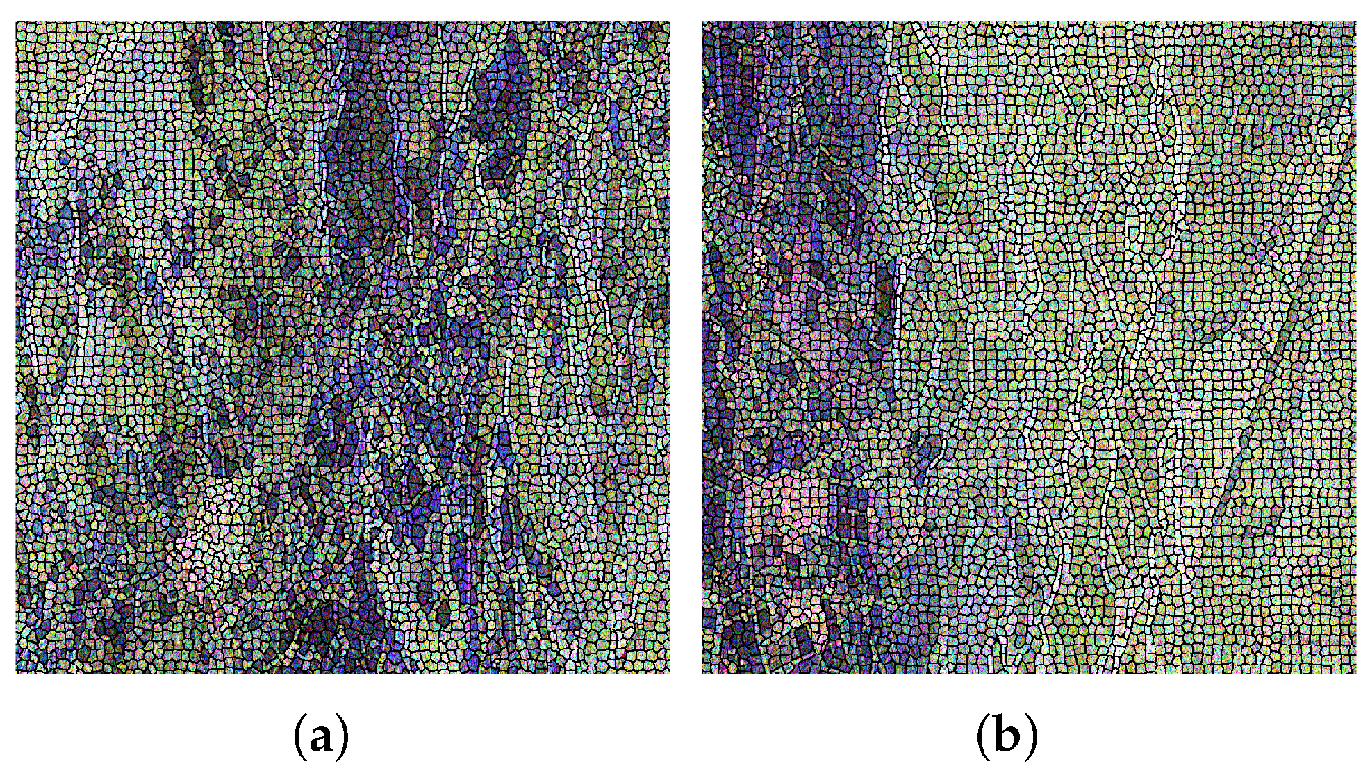
3.2. Homogeneous Patch Segmentation

Among various segmentation methods, simple linear iterative clustering (SLIC) offers a lower computational cost and memory efficiency [39]. However, the presence of speckle noise in SAR imagery reduces its effectiveness. To address this, the similarity metric must be adapted accordingly.

Let ${\widehat{R}}_x$ and ${\widehat{R}}_y$ be complex-Wishart-distributed, i.e., ${\widehat{R}}_x\in W_c(N_x,R_x)$ and ${\widehat{R}}_y\in W_c(N_y,R_y)$, and $R_x$ and $R_y$ are the center covariance matrices, respectively. To determine whether two pixels belong to the same homogeneous region, the following hypothesis test is formulated:

$$\left\{\begin{array}{c}{H}_0:R_x=R_y=R\hfill \\ H_1:R_x\ne R_y.\hfill \end{array}\right.$$

(7)

Under the null hypothesis $H_0$, the likelihood function is

$$L_{H_0}(\widehat{R}\mid R)=\prod _{n=1}^{N_x+N_y}f(\widehat{R};R,N_x+N_y).$$

(8)

Under the alternative hypothesis $H_1$, the joint likelihood becomes

$$\begin{array}{cc}\hfill & L_{H_1}({\widehat{R}}_x,{\widehat{R}}_y|R_x,R_y)\hfill \\ \hfill & =\prod _{n=1}^{N_x}f({\widehat{R}}_x;R_x,N_x)\prod _{n=1}^{N_y}f({\widehat{R}}_y;R_y,N_y).\hfill \end{array}$$

(9)

Then, the likelihood-ratio test statistic is given by

$$Q={\displaystyle \frac{L_{H_0}(\widehat{R}\mid R)}{L_{H_1}({\widehat{R}}_x,{\widehat{R}}_y\mid R_x,R_y)}}$$

(10)

Substituting (6), (8), and (9) into (10) yields [42]

$$Q={\displaystyle \frac{|R_x{|}^{N_x}{\left|R_y\right|}^{N_y}}{|R_x+R_y{|}^{N_x+N_y}}}.$$

(11)

Generally, we have $N_x=N_y$ in the covariance matrix estimation. Then, the hypothesis test distance measure can be defined by taking the natural logarithm on (11):

$$d_P=ln|R_x|+ln|R_y|-2ln|R_x+R_y|.$$

(12)

The distance metric between the PolSAR pixels should consider both scattering similarity and spatial distance to produce compact patches that adhere well to image boundaries. Therefore, the two distances are combined as [34]

$$D=\sqrt{{d_P}^2+{\left({\displaystyle \frac{d_s}{S}}\right)}^2{m}^2}$$

(13)

where S is the grid interval, and $d_s$ is the spatial Euclidean distance between the pixels, and constant m weighs the relative importance between Wishart similarity $d_P$ and spatial distance $d_s$. To reduce the computational complexity, the $6\times 6$ covariance matrix R can be replaced with the $3\times 3$ coherence matrix T, which is also complex-Wishart-distributed.

3.3. Covariance Matrix Re-Estimation

To reduce the influence of the non-homogeneous scatterers, the covariance matrix can be estimated by assigning the homogeneous pixels with weights [43]:

$$w={\displaystyle \frac{1}{W}}exp(-{\displaystyle \frac{d_s}{S}})$$

(14)

where $W={\sum }_i{w}_i$ is a normalization factor ensuring that the total weight sums to 1. To estimate the covariance matrix, one first needs to define the size of the grid interval and multilook window. For the center pixel, only the pixels at the intersection of the patch and the multilook window are assigned corresponding weights. Figure 2 shows an example to illustrate the covariance matrix estimation.

Then, the polarimetric coherency matrices $T_i$ and polarimetric interferometry matrix $\Omega$ can be estimated as

$$T_i=\sum _{n=1}^{N}w\left(n\right)〈k_{i,n}{k}_{i,n}^H〉,\Omega =\sum _{n=1}^{N}w\left(n\right)〈k_{1,n}{k}_{2,n}^H〉.$$

(15)

4. Joint-Pixel Optimization Inversion

This section presents the formulation of joint pixel optimization, the proposed parallelizable alternating direction method of multipliers (ADMM), and the corresponding inversion scheme.

For individual pixels, the ground phase estimation in the pixel-based method is formulated as an optimization problem, which can be simplified as

$$\varphi =\underset{\varphi }{\mathrm{argmin}}f\left(\varphi \right).$$

(16)

However, this formulation does not account for the dependency between neighboring pixels. To jointly process pixels within the same homogeneous patch, one approach is to aggregate the objective functions of the individual elements as

$$\underset{\varphi }{min}\sum _{i=1}^n{f}_i\left({\varphi }_i\right).$$

(17)

Nevertheless, the above formulation does not fully consider the dependence between pixels. The homogeneous characteristic can incorporate the prior knowledge of the imaged scene or assert a certain desired smoothness for the solution [33]. Here, a first-order regularization model is considered to penalize the variations of the surface from ${\nabla }_x\varphi =0$ and ${\nabla }_y\varphi =0$ by minimizing

$$r\left(\varphi \right)=\sum \sum \left|{\nabla }_x\varphi \right|+\left|{\nabla }_y\varphi \right|,$$

(18)

where x and y are the spatial coordinates, and the sum is calculated in the neighborhood of homogeneous pixels.

For the convenience of formulation, it is assumed that the patch is one-dimensional and will be expanded to a two-dimensional one later. Under this assumption, the regularization term is written as

$$r\left(\varphi \right)=\sum \left|\nabla \varphi \right|=\sum _{i=1}^{n-1}\left|{\varphi }_i-{\varphi }_{i+1}\right|,$$

(19)

where n is the pixel number of the patch.

Combining (17) and (19) yields the new joint-pixel optimization:

$$\underset{\varphi }{min}\sum _{i=1}^n{f}_i\left({\varphi }_i\right)+\mu \sum _{i=1}^{n-1}\left|{\varphi }_i-{\varphi }_{i+1}\right|$$

(20)

where $\mu$ is a penalty coefficient.

Firstly, the coefficient matrix F is defined to simplify the derivations in our later analysis. The regularization term can be expressed in a vectorized form as

$$\begin{array}{cc}\hfill & \sum _{i=1}^{n-1}\left|{\varphi }_i-{\varphi }_{i+1}\right|\hfill \\ \hfill & =\left[\begin{array}{cccccc}1& -1& 0& \dots & 0& 0\\ 0& 1& -1& \dots & 0& 0\\ ⋮& ⋮& ⋮& \ddots & ⋮& ⋮\\ 0& 0& 0& \dots & 1& -1\end{array}\right]\left[\begin{array}{c}{\varphi }_1\\ {\varphi }_2\\ ⋮\\ {\varphi }_n\end{array}\right]\hfill \\ \hfill & ={\parallel F\varphi \parallel }_1\hfill \end{array}$$

(21)

where $F\in {\mathbb{R}}^{n_r\times n}$, $\varphi \in {\mathbb{R}}^n$ is the ground phase vector, and ${\parallel ·\parallel }_1$ denotes the 1-norm. Note that $n_r$ represents the number of regularization terms, and n denotes the number of pixels within the patch.

Based on the new formulation (21), the objective function in (20) can be reformulated as

$$\underset{\varphi }{min}f\left(\varphi \right)+\mu {\parallel F\varphi \parallel }_1$$

(22)

where $f\left(\varphi \right)={\displaystyle \sum _{i=1}^n}{f}_i\left({\varphi }_i\right)$. A new variable z and an equality constraint $F\varphi -z=0$ are introduced to obtain the equivalent optimization problem of (22)

$$\begin{array}{c}minf\left(\varphi \right)+\mu {\parallel z\parallel }_1\hfill \\ \begin{array}{cc}s.t& F\varphi -z=0.\end{array}\hfill \end{array}$$

(23)

The augmented Lagrangian function for the problem (23) is given by

$$L\left(\varphi ,z,\lambda \right)=f\left(\varphi \right)+\mu {\parallel z\parallel }_1+{\lambda }^T\left(F\varphi -z\right)+{\displaystyle \frac{\rho }{2}}{\parallel F\varphi -z\parallel }^2$$

(24)

where $\lambda \in {\mathbb{R}}^{n_r}$. Applying the alternating direction method of multipliers (ADMM) yields the iterative updates [44,45]:

$$\begin{array}{cc}\hfill {\varphi }^{k+1}& =\underset{\varphi }{\mathrm{argmin}}L\left(\varphi ,z^k,{\lambda }^k\right)\hfill \\ \hfill z^{k+1}& =\underset{z}{\mathrm{argmin}}L\left({\varphi }^k,z,{\lambda }^k\right)\hfill \\ \hfill {\lambda }^{k+1}& ={\lambda }^k+{\alpha }^k\left(F{\varphi }^{k+1}-z^{k+1}\right)\hfill \end{array}$$

(25)

Simplifying the objective function of the first equality in the above updates yields

$$\sum _{i=1}^n{f}_i\left({\varphi }_i\right)+{\lambda }^T\left(F\varphi -z^k\right)+{\displaystyle \frac{\rho }{2}}\parallel F\varphi -z^k{\parallel }^2.$$

(26)

This expression is not separable due to the penalty term, which prevents parallel optimization over individual variables. In order to solve this problem, we design a new iterative algorithm that enables parallel decomposition for (24). Details of the algorithm and its convergence analysis are provided in Appendix A. According to the algorithm provided in Appendix A, the iteration steps can be written as

$$\begin{array}{cc}\hfill {\varphi }^{k+1}& =\underset{\varphi }{\mathrm{argmin}}f\left(\varphi \right)-{\left({\lambda }^k\right)}^{T}F\varphi +{\displaystyle \frac{\tau }{2}}\parallel \varphi -{\varphi }^k{\parallel }^2\hfill \\ \hfill z^{k+1}& =\underset{z}{\mathrm{argmin}}\mu {\parallel z\parallel }_1-{\left({\lambda }^k\right)}^{T}z+{\displaystyle \frac{\sigma }{2}}\parallel z-z^k{\parallel }^2\hfill \\ \hfill {\lambda }^{k+1}& ={\lambda }^k-{\alpha }^{-1}\left\{F(2{\varphi }^{k+1}-{\varphi }^k)-(2z^{k+1}-z^k)\right\}\hfill \end{array}$$

(27)

where $\tau$, $\sigma$, and $\alpha$ are positive numbers. From the variational inequality derived from (27), the matrix Q [see Appendix A] is expressed as

$$Q=\left[\begin{array}{ccccc}\sigma & 0& \dots & 0& 1\\ 0& \tau & \dots & 0& F_1^T\\ ⋮& ⋮& \ddots & ⋮& ⋮\\ 0& 0& \dots & \tau & F_n^T\\ 1& F_1& \dots & F_n& \alpha \end{array}\right].$$

(28)

To guarantee the positive semi-definiteness of Q, the following condition must hold:

$$\alpha -{\displaystyle \frac{1}{\sigma }}-{\displaystyle \frac{1}{\tau }}\sum _{i=1}^n{F}_i^T{F}_i\ge 0\Rightarrow \alpha \ge {\displaystyle \frac{1}{\tau }}\parallel F^{T}F\parallel +{\displaystyle \frac{1}{\sigma }}.$$

(29)

Accordingly, the update step for $\varphi$ in (27) simplifies to the following:

$$\begin{array}{cc}\hfill & {\varphi }^{k+1}=\underset{{\varphi }_i}{\mathrm{argmin}}\sum _{i=1}^n{f}_i\left({\varphi }_i\right)-{\left(F^T{\lambda }^k\right)}^T\varphi +{\displaystyle \frac{\tau }{2}}\parallel \varphi -{\varphi }^k{\parallel }^2\hfill \\ \hfill & =\underset{{\varphi }_i}{\mathrm{argmin}}\sum _{i=1}^n{f}_i\left({\varphi }_i\right)-{\left(F^T{\lambda }^k\right)}_i^T{\varphi }_i+{\displaystyle \frac{\tau }{2}}{({\varphi }_i-{\varphi }_i^k)}^2.\hfill \end{array}$$

(30)

Equation (30) clearly indicates that this minimization problem decouples into n independent subproblems, which can be solved in parallel.

The update of z can be reformulated using a proximal operator:

$$\begin{array}{cc}\hfill z^{k+1}& =\underset{z}{\mathrm{argmin}}\mu {\parallel z\parallel }_1+{\displaystyle \frac{\sigma }{2}}\parallel z-z^k+{\displaystyle \frac{{\lambda }^k}{\sigma }}{\parallel }^2\hfill \\ \hfill & =\underset{z}{\mathrm{argmin}}{\displaystyle \frac{\mu }{\sigma }}{\parallel z\parallel }_1+{\displaystyle \frac{1}{2}}\parallel z-(z^k-{\displaystyle \frac{{\lambda }^k}{\sigma }}){\parallel }^2\hfill \\ \hfill & =\mathrm{Pro}{\mathrm{x}}_{{\displaystyle \frac{\mu }{\sigma }}{\parallel ·\parallel }_1}(z^k-{\displaystyle \frac{{\lambda }^k}{\sigma }}).\hfill \end{array}$$

(31)

The analytical solution to (31) is given by [46]

$$z^{k+1}=\mathrm{sign}(z^k-{\displaystyle \frac{{\lambda }^k}{\sigma }})max\{|z^k-{\displaystyle \frac{{\lambda }^k}{\sigma }}|-{\displaystyle \frac{\mu }{\sigma }},0\}.$$

(32)

Combining (30) and (32), the update of $\lambda$ in (27) becomes straightforward. Once the ground phase is determined, the forest height can be estimated using the RVoG inversion approach described in Section 3.

The convergence of the iterative algorithm is analyzed with regard to the separable equality-constrained convex optimization problem. However, the convergence should be further specified, as the objective function in a MAP estimate is non-convex. Recent research has shown the convergence of the ADMM for a variety of non-convex functions [45]. Although the corresponding conditions are very difficult to prove theoretically, the proposed iterative algorithm shows good convergence properties. The norm of the residual ${\parallel F\varphi -z\parallel }_1$ for each iteration is calculated and presented in the experimental results.

In Formulation (19), homogeneous patches are initially modeled as one-dimensional for simplification. However, since segmented patches are typically irregular in shape, enforcing a linear pixel order can disrupt spatial continuity. A more natural extension to two-dimensional (2D) space better captures the patch structure. The regularization item satisfies several rules. Firstly, each pixel within the same patch is assigned a unique column-wise numerical identifier, and regularization terms are computed sequentially based on these identifiers. Specifically, each pixel selectively computes its regularization term exclusively with the pixel possessing the minimal Euclidean distance among those pixels with a greater sequential identifier. Additionally, each regulation term is weighted by the reciprocal of the Euclidean distance between the involved pixels. This weighting mechanism ensures that the contribution of each regularization term is proportionate to the spatial similarity.

Figure 3 provides an example of an irregular patch with nine pixels to illustrate the process of calculating the regularization terms. According to the rules, there are 11 regularization terms in total. Among these, only the fifth and eleventh terms have a coefficient of $1/\phantom{1\sqrt{2}}\sqrt{2}$, while the remaining terms have coefficients of 1. The modification of regularization terms can be conveniently achieved by adjusting the coefficient matrix F.

The complete process for joint-pixel optimization is outlined in Algorithm 1.

Algorithm 1 Joint-Pixel Optimization for PolInSAR

1: Input: Segmented covariance matrix T, matrix $\Omega$, topographic phase ${\varphi }_{topo}$, maximum number of iterations ${\mathrm{Iter}}_{\max }$, and the threshold $\mathrm{Thr}$. 2: Initialize the iterative parameters $\tau$ and $\sigma$ with random positive values. 3: for $\mathit{iter}<{\mathrm{Iter}}_{\max }$ do 4:    Compute the coefficient matrix F; 5:    Initialize $\alpha$ according to (29); 6:    Initialize ${\varphi }^0$ with a topographic phase, set $z^0=F{\varphi }^0$, and randomly initialize ${\lambda }^0$; 7:    Estimate each ground phase ${\varphi }_i$ using the golden section search method (30); 8:    Update z and $\lambda$ in (32) and (27), respectively; 9:    if $\parallel {\varphi }^{\mathrm{iter}}-{\varphi }^{\mathrm{iter}-1}{\parallel }_Q<\mathrm{Thr}$ then 10:      break 11:    end if 12: end for

5. Experiments and Discussion

5.1. Data Preprocessing

The overall inversion workflow is illustrated in Figure 4. The preprocessing stage includes the extraction of SAR imagery, image coregistration, projecting the external DEM to the slant range geometry, estimation of the key parameters, and flat earth phase removal. The coregistration is performed in the correlation coefficient method, and its accuracy is 0.013 pixels in range and 0.036 pixels. This corresponds to approximately 0.049 m and 0.133 m, respectively, given the pixel spacings of 3.75 m (range) and 3.70 m (azimuth). The external DEM is transformed into the slant range coordinate system to facilitate the key parameter estimations, including perpendicular baseline, flat earth phase, terrain-corrected vertical wavenumber, and topographic phase. The variation in the perpendicular baseline is relatively small, ranging from 895 to 912 m in the whole scene. In the test site, the vertical wavenumber ranges from 0.16 to 0.185 (rad/m). Then, the flat-earth phase can be removed for slave images.

To further validate the effectiveness of homogeneous patch segmentation, two small areas are zoomed in to see the actual scattering mechanisms within the homogeneous patch. Figure 5 presents the locally segmented results with a grid interval $S=15$, superimposed on the Pauli-based color composite images. The compact, irregular black superpixels represent the segmented patches. Notably, the patches adhere closely to the image boundaries, showcasing a good edge-preserving effect. Moreover, the pixels within the segmented patches exhibit uniform colors, indicating a similarity in the underlying scattering mechanisms.

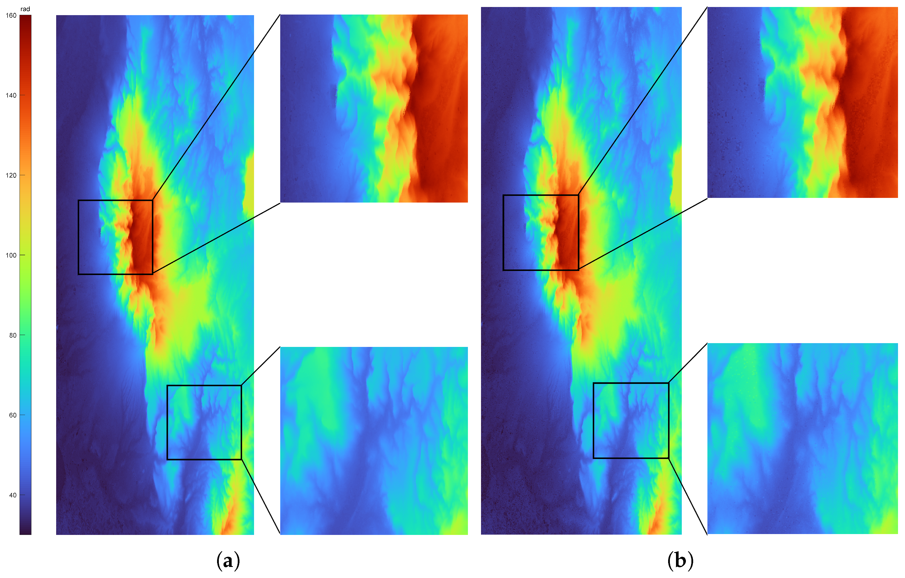
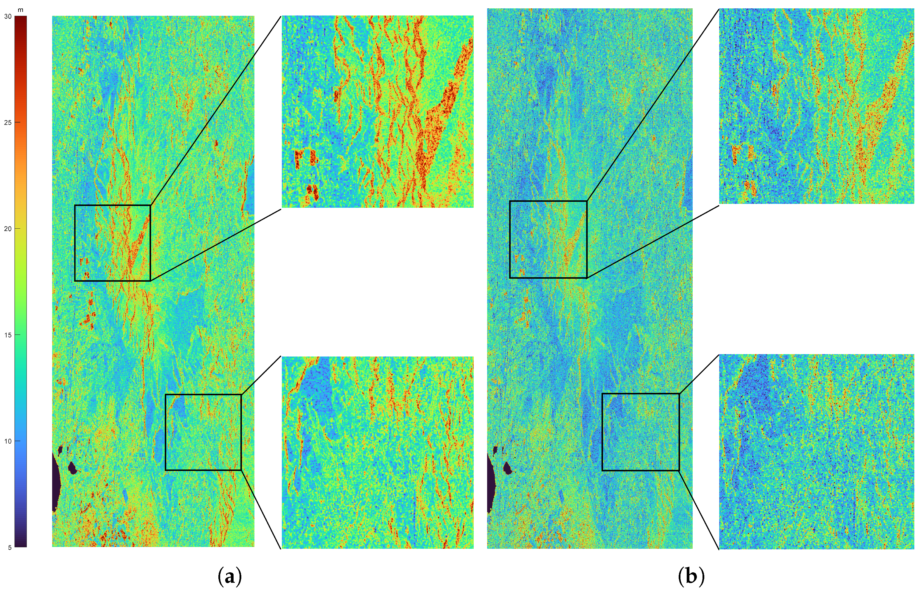
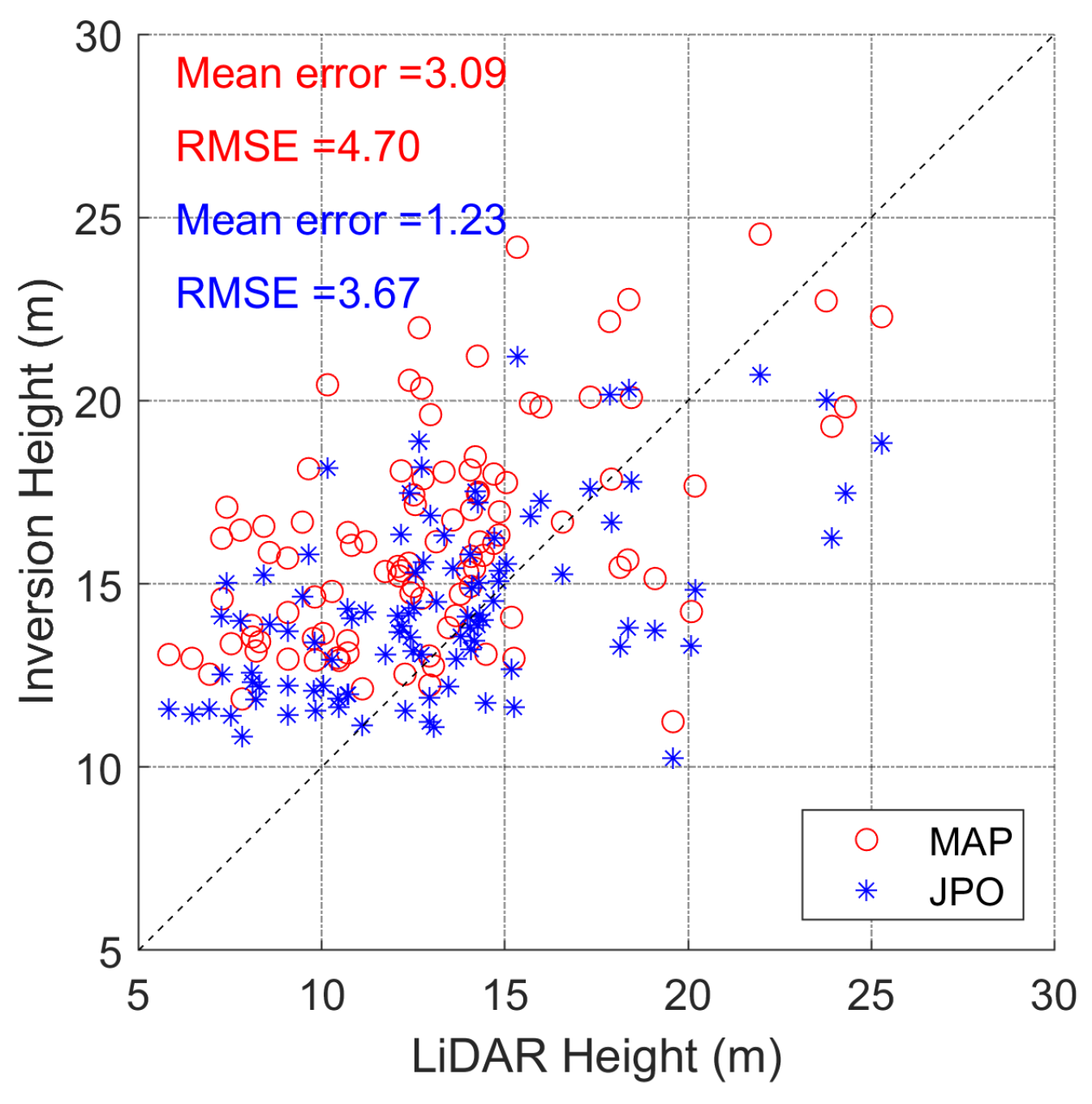
5.2. Inversion and Validation

The forest height estimation is performed using the proposed JPO method and the pixel-based method, maximum a posteriori inversion [30] (referred to MAP), respectively. In both methods, the multilook window and the grid interval are 7 pixels. In JPO, the iterative parameters $\mu ,\tau$ are set to 1, and ${\lambda }_0$ and $\sigma$ are both random numbers. In the segmentation, the constant m is determined by the compactness [39] of the patch, which is fixed to 1 in the experiments. The optimization of $\varphi$ in each separate problem is solved using the golden-section search method, with the topographic phase serving as the initial value [30,47].

Figure 6 shows the estimated ground phase from two methods, and the left color bar labeled “rad” indicates phase values in radians. Although the estimated results look visually close, the zoomed-in areas show their local differences. Overall, the ground phase estimated by the MAP method is observed to be smoother compared to that of JPO. Interestingly, it seems somewhat counter-intuitive. Specifically, the JPO method employs phase continuity constraints to regularize the joint-processed pixels, which should improve phase continuity. It is found that this phenomenon is mainly caused by the different covariance estimations in the two methods. The MAP method utilizes a boxcar filter that assigns equal weights to all pixels without assessing their similarity, leading to smoother but less localized results. In contrast, the JPO approach re-estimates the covariance matrix based on segmented patches, thereby preserving a more localized variation at the cost of overall smoothness. This phenomenon is discussed later.

Figure 7 shows the estimated heights from two methods. Although the trends of the estimated results are very close, the MAP method shows an obvious overestimation phenomenon than the JPO method. To validate these results, the sparse ICESat-2 LiDAR data, which are referenced to the WGS-84 coordinate system, are used as the ground truth. The PolInSAR height maps are first geocoded to the WGS-84 system with a pixel spacing of approximately 10 m. Subsequently, the ICESat-2 height maps are constructed according to the specific referencing information from the projected PolInSAR height map. The LiDAR heights of all segments are mapped to the geographic coordinates using the nearest neighbor algorithm based on the longitude and latitude. Figure 8 presents the geocoded height maps and the corresponding difference maps between the estimated heights and the LiDAR heights. Specifically, the dots represent the error between the estimated height and the reference height at the corresponding pixel.

As shown in Figure 8, the MAP-based results exhibit more substantial errors, as evidenced by the increased density of red-colored dots in panel (a) compared to panel (b). Figure 9 further visualizes the differences through histograms of estimation error. The left-skewed distributions in Figure 9 indicate a tendency for overestimation of the estimated heights compared with the LiDAR heights. The mean error of both methods lies on the positive side, confirming a consistent bias in predictions. It should be emphasized that accurate height inversion is feasible only within a limited range of forest heights due to the relatively small variation in vertical wavenumber across the scene from 0.16 to 0.185 (rad/m). As a result, both methods exhibit varying degrees of overestimation.

Figure 10 presents correlation plots comparing PolInSAR-derived heights with ICESat-2 reference measurements. A quantitative evaluation reveals that the JPO method achieves a mean error of 1.23 m and an RMSE of 3.67 m, while the MAP method yields a mean error of 3.09 m and an RMSE of 4.70 m. The reduced mean error and RMSE demonstrate improved prediction reliability. Overall, the JPO method exhibits a significant improvement over the MAP methods and effectively reduces overestimation.

5.3. Discussion

The center pixel of the entire image is selected to illustrate the convergence. Figure 11 displays the residual ${\parallel F\varphi -z\parallel }_1$ at each iteration during the joint-pixel optimization. The fourth iteration satisfies the stopping criterion, where the residual is less than 0.1 degrees for each pixel. The residual curve demonstrates the effectiveness and stability of the proposed iterative algorithm.

Next, the decorrelation effects caused by non-homologous scattering are analyzed from the estimated volume coherence. Similarly, Figure 12 illustrates two localized examples of the estimated volume coherence obtained from the JPO and MAP methods. In Figure 12a,b, the boxcar filtering in covariance matrix estimation effectively reduces the speckle noise. However, it comes at a cost of loss of fine details due to blurring. On the other hand, the results from the JPO method show significant speckle noise reduction and well-preserved details. The main difference is twofold. The covariance matrix estimation of the JPO method is unfolded within the similarity patch, and the involved pixels are weighted according to the spatial distance. It reduces the additional decorrelation due to the presence of non-identical scatterings. Consequently, the estimated volume coherence in the JPO method is generally higher than that of the MAP method.

The grid interval S plays an important role in the proposed method as it determines the approximate size of the segmented patch. A small grid interval results in poorer suppression of speckle noise, while a large grid interval may lead to a failed constraint on the surface due to the relatively large phase variance of the involved pixels. The complexity of homogeneous patch segmentation is linear with respect to the pixel number of the whole image, irrespective of S [39]. Therefore, the time required to segment images remains unaffected by the choice of S. Additionally, the later computational complexity analysis indicates that the complexity of the inversion is slightly affected by S. A set of experiments is conducted to investigate the impact of varying grid intervals on the estimation of the ground phase. In the experiments, the grid intervals are systematically set to 5, 7, 9, 11, 13, and 15, respectively. In the re-estimation of the covariance matrix, a fixed window size of 7 pixels is maintained for the ensemble average of covariance matrix estimation, with equal weighting assigned to pixels. This deliberate design aims to standardize the covariance matrix estimation, allowing for a more focused analysis of the unique effects introduced by different grid intervals on the ground phase estimation. Figure 13 and Figure 14 show the estimated ground phase by JPO with different grid intervals in two local areas. The results show that when the grid interval is relatively small, some pixels within otherwise smooth regions may exhibit noticeable deviations from their neighbors. Conversely, using a larger grid interval can introduce the visible block-like effect, likely due to joint optimization over a broader set of pixels that may not be truly homogeneous. Despite these variations, the overall visual differences remain minor across settings, highlighting the algorithm’s robustness to changes in the grid interval parameter.

Several parameters are involved in the joint optimization process, $\mu$, $\tau$, $\sigma$, and $\alpha$. The regularization parameter $\mu$ controls the significance of the consistency constraint. Specifically, a larger $\mu$ indicates that the optimization prefers to search the optimal within the consistent gradient fields. The parameter $\tau$ is used to enforce strong convexity of the objective function near the optimum, thereby accelerating the convergence of the algorithm. Another parameter $\alpha$ must satisfy the positive regularity condition (29) once $\tau$ has been randomly determined.

The computational complexity of the proposed JPO method comprises three main components: homogeneous patch segmentation, re-estimation of the covariance matrix, and joint-pixel optimization. As the complexity of the segmentation step is linear with respect to the total number of pixels [39], we focus our analysis on the computational cost of covariance matrix re-estimation and joint-pixel optimization, in comparison to the pixel-based MAP inversion. For a SAR image of size $N_l\times N_c$, let $n_s$ denote the number of samples in the look-up table used for ground phase estimation. The computational burden of the pixel-based processing in MAP is $N_l\times N_c\times (W^2{T}_{OR}+n_s{T}_{OG}+T_I)$, where W is the multilook window; $T_{OR}$, $T_{OG}$, and $T_I$ denote the calculation time of the covariance matrix, the phase estimation at a sampling point, and the inversion. Similarly, the computational burden of the patch-based is $N_l\times N_c/S^2\times (p{S}^2{T}_{OR}+S^2{n}_1{n}_2{T}_{OG}+S^2{T}_I)$, where S is the grid interval, p represents the ratio of the pixels in the search window and the center pixel belonging to the same patch, $n_1$ is the number of sampling points for each pixel in one iteration, and $n_2$ represents the number of iterations. The experiments show that $n_1{n}_2\approx n_s$ when the sampling accuracy of the ground phase is consistent. Therefore, the computational burden of patch-based processing is approximately equal to that of pixel-based processing.

6. Conclusions

In this paper, a new patch-based forest height inversion method referred to as JPO is proposed by taking advantage of the neighboring information. The key steps, including homogeneous patch segmentation, re-estimation of the covariance matrix, and joint pixel optimization, are introduced and integrated into JPO. With the contextual information of neighboring pixels, JPO is able to provide reliable forest height estimation and reduce the additional decorrelation. Quantitative evaluations in forest height estimation show that the proposed method achieves a lower mean error (1.23 m) and RMSE (3.67 m) than the MAP method (mean error: 3.09 m; RMSE: 4.70 m), demonstrating its improved reliability. However, the small variation in vertical wavenumber across the scene limits the inversion accuracy. Additionally, the proposed iterative algorithm effectively addresses the non-parallelizable problem of the alternating direction method of multipliers. Future research will focus on the applications of the proposed method in multi-baseline PolInSAR inversion.

References

1. Sheil, D. Forests, atmospheric water and an uncertain future: The new biology of the global water cycle. For. Ecosyst. 2018, 5, 19. [Google Scholar] [CrossRef]
2. Mitchard, E.T.A. The tropical forest carbon cycle and climate change. Nature 2018, 559, 527–534. [Google Scholar] [CrossRef]
3. Yin, T.; Montesano, P.M.; Cook, B.D.; Chavanon, E.; Neigh, C.S.; Shean, D.; Peng, D.; Lauret, N.; Mkaouar, A.; Morton, D.C.; et al. Modeling forest canopy surface retrievals using very high-resolution spaceborne stereogrammetry: (I) methods and comparisons with actual data. Remote Sens. Environ. 2023, 298, 113825. [Google Scholar] [CrossRef]
4. Liao, Z.; He, B.; Quan, X.; van Dijk, A.I.J.M.; Qiu, S.; Yin, C. Biomass estimation in dense tropical forest using multiple information from single-baseline P-band PolInSAR data. Remote Sens. Environ. 2019, 221, 489–507. [Google Scholar] [CrossRef]
5. Treuhaft, R.; Goncalves, F.; dos Santos, J.R.; Keller, M.; Palace, M.; Madsen, S.N.; Sullivan, F.; Graca, P.M.L.A. Tropical-Forest Biomass Estimation at X-Band From the Spaceborne TanDEM-X Interferometer. IEEE Geosci. Remote Sens. Lett. 2015, 12, 239–243. [Google Scholar] [CrossRef]
6. Le Toan, T.; Quegan, S.; Davidson, M.W.J.; Balzter, H.; Paillou, P.; Papathanassiou, K.; Plummer, S.; Rocca, F.; Saatchi, S.; Shugart, H. The BIOMASS mission: Mapping global forest biomass to better understand the terrestrial carbon cycle. Remote Sens. Environ. 2011, 115, 2850–2860. [Google Scholar] [CrossRef]
7. West, P.W. Tree Height. In Tree and Forest Measurement; Springer International Publishing: Cham, Switzerland, 2015; pp. 19–24. [Google Scholar] [CrossRef]
8. Zhu, X.; Nie, S.; Wang, C.; Xi, X.; Lao, J.; Li, D. Consistency analysis of forest height retrievals between GEDI and ICESat-2. Remote Sens. Environ. 2022, 281, 113244. [Google Scholar] [CrossRef]
9. Hajnsek, I.; Kugler, F.; Lee, S.; Papathanassiou, K.P. Tropical-Forest-Parameter Estimation by Means of Pol-InSAR: The INDREX-II Campaign. IEEE Trans. Geosci. Remote Sens. 2009, 47, 481–493. [Google Scholar] [CrossRef]
10. Dubois-Fernandez, P.C.; Le Toan, T.; Daniel, S.; Oriot, H.; Chave, J.; Blanc, L.; Villard, L.; Davidson, M.W.; Petit, M. The TropiSAR airborne campaign in French Guiana: Objectives, description, and observed temporal behavior of the backscatter signal. IEEE Trans. Geosci. Remote Sens. 2012, 50, 3228–3241. [Google Scholar] [CrossRef]
11. Potapov, P.; Li, X.; Hernandez-Serna, A.; Tyukavina, A.; Hansen, M.C.; Kommareddy, A.; Pickens, A.; Turubanova, S.; Tang, H.; Silva, C.E.; et al. Mapping global forest canopy height through integration of GEDI and Landsat data. Remote Sens. Environ. 2021, 253, 112165. [Google Scholar] [CrossRef]
12. Li, W.; Niu, Z.; Shang, R.; Qin, Y.; Wang, L.; Chen, H. High-resolution mapping of forest canopy height using machine learning by coupling ICESat-2 LiDAR with Sentinel-1, Sentinel-2 and Landsat-8 data. Int. J. Appl. Earth Obs. Geoinf. 2020, 92, 102163. [Google Scholar] [CrossRef]
13. García, M.; Saatchi, S.; Ustin, S.; Balzter, H. Modelling forest canopy height by integrating airborne LiDAR samples with satellite Radar and multispectral imagery. Int. J. Appl. Earth Obs. Geoinf. 2018, 66, 159–173. [Google Scholar] [CrossRef]
14. Pourshamsi, M.; Xia, J.; Yokoya, N.; Garcia, M.; Lavalle, M.; Pottier, E.; Balzter, H. Tropical forest canopy height estimation from combined polarimetric SAR and LiDAR using machine-learning. ISPRS J. Photogramm. Remote Sens. 2021, 172, 79–94. [Google Scholar] [CrossRef]
15. Kugler, F.; Lee, S.; Hajnsek, I.; Papathanassiou, K.P. Forest Height Estimation by Means of Pol-InSAR Data Inversion: The Role of the Vertical Wavenumber. IEEE Trans. Geosci. Remote Sens. 2015, 53, 5294–5311. [Google Scholar] [CrossRef]
16. Garestier, F.; Dubois-Fernandez, P.C.; Champion, I. Forest height inversion using high-resolution P-band Pol-InSAR data. IEEE Trans. Geosci. Remote Sens. 2008, 46, 3544–3559. [Google Scholar] [CrossRef]
17. Zhao, L.; Chen, E.; Li, Z.; Zhang, W.; Fan, Y. A New Approach for Forest Height Inversion Using X-Band Single-Pass InSAR Coherence Data. IEEE Trans. Geosci. Remote Sens. 2021, 60, 5206018. [Google Scholar] [CrossRef]
18. Cloude, S.R.; Papathanassiou, K.P. Polarimetric SAR interferometry. IEEE Trans. Geosci. Remote Sens. 1998, 36, 1551–1565. [Google Scholar] [CrossRef]
19. Cloude, S.R. Pol-InSAR training course. In Radio Science; Blackwell Publishing: Hoboken, NJ, USA, 2005. [Google Scholar]
20. Treuhaft, R.N.; Chapman, B.D.; dos Santos, J.R.; Dutra, L.V.; Goncalves, F.G.; Freitas, C.d.C.; Mura, J.C.; de Alencastro Graca, P.M.; Drake, J.B.; IEEE. Tropical-Forest Density Profiles from Multibaseline Interferometric SAR. In Proceedings of the 2006 IEEE International Symposium on Geoscience and Remote Sensing, Denver, CO, USA, 31 July–4 August 2006; pp. 2205–2207. [Google Scholar] [CrossRef]
21. Treuhaft, R.N.; Siqueira, P.R. Vertical structure of vegetated land surfaces from interferometric and polarimetric radar. Radio Sci. 2000, 35, 141–177. [Google Scholar] [CrossRef]
22. Papathanassiou, K.P.; Cloude, S.R. Single-baseline polarimetric SAR interferometry. IEEE Trans. Geosci. Remote Sens. 2001, 39, 2352–2363. [Google Scholar] [CrossRef]
23. Cloude, S.; Papathanassiou, K. Three-stage inversion process for polarimetric SAR interferometry. IEE Proc.-Radar Sonar Navig. 2003, 150, 125–134. [Google Scholar] [CrossRef]
24. Flynn, T.; Tabb, M.; Carande, R. Coherence region shape extraction for vegetation parameter estimation in polarimetric SAR interferometry. In Proceedings of the IEEE International Geoscience and Remote Sensing Symposium, Toronto, ON, Canada, 24–28 June 2002; Volume 5, pp. 2596–2598. [Google Scholar] [CrossRef]
25. Mark, T.; Jeffrey, O.; Thomas, F.; Richard, C. Phase diversity: A decomposition for vegetation parameter estimation using polarimetric SAR interferometry. In Proceedings of the European Conference on Synthetic Aperture Radar EUSAR, Cologne, Germany, 4–6 June 2002; pp. 721–724. [Google Scholar]
26. Papathanassiou, K.P.; Cloude, S.R. The effect of temporal decorrelation on the inversion of forest parameters from Pol-InSAR data. In Proceedings of the International Geoscience and Remote Sensing Symposium, Toulouse, France, 21–25 July 2003; Volume 3, pp. 1429–1431. [Google Scholar]
27. Mette, T.; Kugler, F.; Papathanassiou, K.; Hajnsek, I. Forest and the random volume over ground-nature and effect of 3 possible error types. In Proceedings of the European Conference on Synthetic Aperture Radar (EUSAR), Dresden, Germany, 16–18 May 2006; VDE Verlag GmbH: Berlin, Germany, 2006; pp. 1–4. [Google Scholar]
28. Lavalle, M.; Hensley, S. Extraction of Structural and Dynamic Properties of Forests from Polarimetric-Interferometric SAR Data Affected by Temporal Decorrelation. IEEE Trans. Geosci. Remote Sens. 2015, 53, 4752–4767. [Google Scholar] [CrossRef]
29. Tabb, M.; Flynn, T.; Carande, R. Full maximum likelihood inversion of PolInSAR scattering models. In Proceedings of the IGARSS 2004, 2004 IEEE International Geoscience and Remote Sensing Symposium, Anchorage, AK, USA, 20–24 September 2004; IEEE: New York, NY, USA, 2004; Volume 2, pp. 1232–1235. [Google Scholar]
30. Huang, Z.; Lv, X.; Li, X.; Chai, H. Maximum a Posteriori Inversion for Forest Height Estimation Using Spaceborne Polarimetric SAR Interferometry. IEEE Trans. Geosci. Remote Sens. 2023, 61, 4406514. [Google Scholar] [CrossRef]
31. Lei, Y.; Siqueira, P.; Torbick, N.; Ducey, M.; Chowdhury, D.; Salas, W. Generation of large-scale moderate-resolution forest height mosaic with spaceborne repeat-pass SAR interferometry and lidar. IEEE Trans. Geosci. Remote Sens. 2018, 57, 770–787. [Google Scholar] [CrossRef]
32. Sun, X.; Wang, B.; Xiang, M.; Zhou, L.; Wang, S.; Jiang, S. Machine-Learning Inversion of Forest Vertical Structure Based on 2-D-SGVBVoG Model for P-Band Pol-InSAR. IEEE Trans. Geosci. Remote Sens. 2022, 60, 5225115. [Google Scholar] [CrossRef]
33. Nico, G.; Palubinskas, G.; Datcu, M. Bayesian approaches to phase unwrapping: Theoretical study. IEEE Trans. Signal Process. 2000, 48, 2545–2556. [Google Scholar] [CrossRef]
34. Qin, F.; Guo, J.; Lang, F. Superpixel segmentation for polarimetric SAR imagery using local iterative clustering. IEEE Geosci. Remote Sens. Lett. 2014, 12, 13–17. [Google Scholar]
35. Guo, Y.; Jiao, L.; Wang, S.; Wang, S.; Liu, F.; Hua, W. Fuzzy superpixels for polarimetric SAR images classification. IEEE Trans. Fuzzy Syst. 2018, 26, 2846–2860. [Google Scholar] [CrossRef]
36. Felzenszwalb, P.F.; Huttenlocher, D.P. Efficient graph-based image segmentation. Int. J. Comput. Vis. 2004, 59, 167–181. [Google Scholar] [CrossRef]
37. Shi, J.; Malik, J. Normalized cuts and image segmentation. IEEE Trans. Pattern Anal. Mach. Intell. 2000, 22, 888–905. [Google Scholar]
38. Veksler, O.; Boykov, Y.; Mehrani, P. Superpixels and supervoxels in an energy optimization framework. In Proceedings of the Computer Vision–ECCV 2010: 11th European Conference on Computer Vision, Heraklion, Crete, Greece, 5–11 September 2010; Proceedings, Part V 11. Springer: Berlin/Heidelberg, Germany, 2010; pp. 211–224. [Google Scholar]
39. Achanta, R.; Shaji, A.; Smith, K.; Lucchi, A.; Fua, P.; Süsstrunk, S. SLIC superpixels compared to state-of-the-art superpixel methods. IEEE Trans. Pattern Anal. Mach. Intell. 2012, 34, 2274–2282. [Google Scholar] [CrossRef]
40. Boyd, S.; Parikh, N.; Chu, E.; Peleato, B.; Eckstein, J. Distributed Optimization and Statistical Learning via the Alternating Direction Method of Multipliers; Foundation Trends® in Machine Learning: Hanover, MA, USA, 2011; Volume 3, pp. 1–122. [Google Scholar]
41. Cloude, S.R. Polarization coherence tomography. Radio Sci. 2006, 41, 1–27. [Google Scholar] [CrossRef]
42. Conradsen, K.; Nielsen, A.A.; Schou, J.; Skriver, H. A test statistic in the complex Wishart distribution and its application to change detection in polarimetric SAR data. IEEE Trans. Geosci. Remote Sens. 2003, 41, 4–19. [Google Scholar] [CrossRef]
43. Lv, X.; Yazıcı, B.; Zeghal, M.; Bennett, V.; Abdoun, T. Joint-scatterer processing for time-series InSAR. IEEE Trans. Geosci. Remote Sens. 2014, 52, 7205–7221. [Google Scholar]
44. Shi, W.; Ling, Q.; Yuan, K.; Wu, G.; Yin, W. On the linear convergence of the ADMM in decentralized consensus optimization. IEEE Trans. Signal Process. 2014, 62, 1750–1761. [Google Scholar] [CrossRef]
45. Wang, Y.; Yin, W.; Zeng, J. Global convergence of ADMM in nonconvex nonsmooth optimization. J. Sci. Comput. 2019, 78, 29–63. [Google Scholar] [CrossRef]
46. Parikh, N.; Boyd, S. Proximal Algorithms; Foundations and Trends® in Optimization: Hanover, MA, USA, 2014; Volume 1, pp. 127–239. [Google Scholar]
47. Kiefer, J. Sequential minimax search for a maximum. Proc. Am. Math. Soc. 1953, 4, 502–506. [Google Scholar] [CrossRef]
48. Kinderlehrer, D.; Stampacchia, G. An Introduction to Variational Inequalities and Their Applications; SIAM: Philadelphia, PA, USA, 2000. [Google Scholar]
49. He, B.; Yuan, X. On non-ergodic convergence rate of Douglas–Rachford alternating direction method of multipliers. Numer. Math. 2015, 130, 567–577. [Google Scholar] [CrossRef]
Figure 1. Distribution of ICESat-2 segments within the study site and a total of 100 homogeneous polygons over the study site.
Remotesensing 17 01726 g001
Figure 2. Illustration of the ensemble average in covariance matrix estimation. The solid red circle is the center pixel, whose covariance matrix needs to be estimated. The red circle indicates that it belongs to the same patch as the center pixel. The black dotted box represents the multilook window centered on the center pixel.
Remotesensing 17 01726 g002
Figure 3. An irregular shape of the patch with homogeneous pixels. The purple circles with red numbers denote the numbered pixels in the patch. The green line with a number denotes the calculated regularization term.
Remotesensing 17 01726 g003
Figure 4. Spaceborne PolInSAR forest height inversion flow.
Remotesensing 17 01726 g004
Figure 5. Segmented results superimposed on the Pauli-based color composite images. Each zoomed-in area covers 1000 × 1000 pixels. (a) First area. (b) Second area.
Remotesensing 17 01726 g005
Figure 6. Estimated ground phase by MAP and JPO, and the maps share the same color bar. (a) MAP. (b) JPO.
Remotesensing 17 01726 g006
Figure 7. Estimated height by MAP and JPO, and the maps share the same color bar. (a) MAP. (b) JPO.
Remotesensing 17 01726 g007
Figure 8. Geocoded forest height maps in the WGS-84 coordinate system and the corresponding difference between the estimated height and the LiDAR height. (a) MAP. (b) JPO.
Remotesensing 17 01726 g008
Figure 9. The difference histogram between the estimated heights and the LiDAR heights. (a) MAP. (b) JPO.
Remotesensing 17 01726 g009
Figure 10. Correlation plots between the PolInSAR height estimates and ICESat-2 heights.
Remotesensing 17 01726 g010
Figure 11. Norm of the residual versus iteration in the joint-pixel optimization of the center pixel. The stopping criterion is satisfied at iteration 4, indicated by the horizontal dashed line.
Remotesensing 17 01726 g011
Figure 12. Estimated volume coherence by MAP and JPO in two local areas, and the maps share the same color bar. (a) MAP in the first area. (b) MAP in the second area. (c) JPO in the first area. (d) JPO in the second area.
Remotesensing 17 01726 g012
Figure 13. Estimated ground phase by JPO with different grid intervals in the first local area, and the maps share the same color bar, as shown in Figure 6. (a) S = 5 . (b) S = 7 . (c) S = 9 . (d) S = 11 . (e) S = 13 . (f) S = 15 .
Remotesensing 17 01726 g013
Figure 14. Estimated ground phase by JPO with different grid intervals in the second local area, and the maps share the same color bar, as shown in Figure 6. (a) S = 5 . (b) S = 7 . (c) S = 9 . (d) S = 11 . (e) S = 13 . (f) S = 15 .
Remotesensing 17 01726 g014
Disclaimer/Publisher’s Note: The statements, opinions and data contained in all publications are solely those of the individual author(s) and contributor(s) and not of MDPI and/or the editor(s). MDPI and/or the editor(s) disclaim responsibility for any injury to people or property resulting from any ideas, methods, instructions or products referred to in the content.