Probabilistic Site Adaptation for High-Accuracy Solar Radiation Datasets in the Western Sichuan Plateau

Abstract

Downward shortwave radiation (DSR) to the Earth’s surface is an essential renewable energy component. Accurate knowledge of solar radiation, i.e., solar energy resource assessment, is a prior requirement for the development of the solar energy industry. In the framework of solar resource assessment, site adaptation refers to leveraging short-term, high-quality ground-based observations as unbiased references to correct long-term, site-specific gridded model datasets, which has been playing an important role in this research area. This study evaluates 12 probabilistic site adaptation (PSA) methods for the correction of the hourly DSR data from multiple gridded DSR products in the Western Sichuan Plateau (WSP). Surface pyranometer observations are used as the reference to adapt predictions from two satellite products and two reanalysis products, collectively. Systematic quantification reveals inherent errors with root mean square errors (RMSEs) > 200 W/m² across all datasets. Through a comparative evaluation of three methodological categories (benchmarking, parametric/non-parametric, and quantile combination approaches), it is demonstrated that quantile-based ensemble methods achieve superior performance. The median ensemble (MED) method delivers optimal error reduction (RMSE: 163.97 W/m², nRMSE: 34.43%). The resulting optimal dataset, with a temporal resolution of 1 h and a spatial resolution of 0.05° × 0.05°, identifies the WSP as a region of exceptional energy potential, characterized by substantial annual total solar radiation (1593.10 kWh/m²/yr) and a stable temporal distribution (negative correlation between the total solar radiation and the coefficient of variation). This methodological framework provides actionable insights for solar resource optimization in complex terrains.

1. Introduction

Solar radiation is one of the key variables in the Earth’s energy budget that determines the climate state and change. Solar energy is also a promising solution to meet the growing demand for renewable energy [1]. The first step in any solar energy project is resource assessment, which provides a means to accurately determine the long-term behavior of solar radiation in order to optimize resource utilization [2,3,4,5]. Accurate and efficient assessment will strongly support the sustainable development of the photovoltaic (PV) industry, which in turn will support the realization of green and low-carbon development goals [6].

Gridded solar radiation products are essential for modern solar resource assessment and prediction. Downward shortwave radiation (DSR) for solar resource assessment can be obtained from three main sources: ground-based observations, satellite remote sensing retrievals, and simulations by numerical weather prediction (NWP) models [4,7,8]. While ground-based observations are highly accurate, they are often limited in spatial coverage and typically available only for short periods of time at a specific site [9]. In contrast, satellite remote sensing retrievals of DSR provide continuous spatial and temporal coverage [3]. Examples of such satellite products include the Fengyun-4 (FY-4), Himawari-8 (H08), the Geostationary Operational Environmental Satellite-R series (GOES-R), and the Clouds and the Earth’s Radiant Energy System (CERES) [10,11], to name just a few. NWP models estimate DSR as part of their output. Data assimilation techniques integrate both historical and real-time observational data to optimize the initial conditions for these models [12,13,14]. The most widely used DSR datasets, such as ERA from the European Centre for Medium-Range Weather Forecasts (ECMWF) and the Modern-Era Retrospective analysis for Research and Applications (MERRA) are reanalysis products generated by combining NWP models with advanced data assimilation systems. However, their relatively coarse resolution may limit their application in studies requiring high spatial detail.

Compared to ground-based observations, satellite and reanalysis DSR products show different biases and uncertainties in different areas [15,16,17,18]. For instance, validation of six satellite-derived hourly DSR products from 57 Baseline Solar Radiation Network (BSRN) sites over 27 years showed biases ranging from −89.04 W/m² to 77.01 W/m² [13]. Zhang et al. [18] found that the global monthly DSR biases between the five reanalysis products and ground-based observations ranged from 11.25 W/m² to 49.80 W/m². Given the inherent strengths and limitations of these products, data-fusion techniques are critical for solar resource assessment and prediction [19,20,21].

The development of satellite remote sensing techniques and data analysis methods has shown their great potential for solar radiation analysis, especially the preprocessed algorithm probabilistic site adaptation (PSA) [3,9]. At the same time, due to geographical and economic constraints, there is a lack of long-term ground-based observations in most areas with abundant solar resources in China [22,23,24]. This limitation poses challenges for accurate solar resource assessment and hinders the development of solar energy projects in these areas.

The application of a correction method to gridded DSR products by using site measurements, commonly referred to site adaptation, is widely used in the solar energy industry [25,26]. The primary aim of site adaptation is to use short-term, high-quality ground-based observations as unbiased references to correct long-term, site-specific gridded model datasets [9,21]. Typically, site adaptation is performed on a single gridded dataset [26,27]. Linear regression and quantile mapping stand out as widely used techniques for site adaptation [27,28]. However, these methods typically combine all observed errors into a single pool and resample from it unconditionally, leading to a lack of discrimination [9]. In other words, these methods lack the capacity to dynamically adapt to changing conditions. In view of the above drawbacks of traditional site adaptation techniques, Yang and Gueymard [9] proposed the PSA method. PSA has two major advantages over traditional site adaptation: (1) it uses multiple gridded datasets in parallel, thereby mitigating the potential risk of dataset selection; (2) a probabilistic representation of site adaptation for atmospheric variables is provided, which enhances the quantification of uncertainty and provides more information about the prediction.

In this study, we adopt the idea proposed by Yang and Gueymard [9] to improve DSR accuracy in the Western Sichuan Plateau (WSP). The WSP contributes 90.14% of Sichuan Province’s PV power stations [29]. Due to the high elevation and relatively low aerosol load, solar radiation in the WSP suffers minimal loss during transmission through the atmosphere, with an annual total solar radiation (TSR) of 1666.8 kWh/m² [24,30]. A DSR dataset for the region is provided using PSA methods.

This paper is organized as follows: data and methods are introduced in Section 2; Section 3 evaluates and compares the effectiveness of the 12 PSA methods in the WSP using ground-based observations, followed by the generation of solar resource maps with the optimal method; Section 4 presents the discussion of the study; conclusions follow in Section 5.

2. Materials and Methods

2.1. Research Area

This study focuses on the WSP (as shown in Figure 1), which is located between 26.05–34.32°N and 97.35–104.43°E, with elevations above 3000 m. The WSP belongs to the plateau mountain climate, with a mean temperature of 4–12 °C, a mean precipitation of 520–900 mm [31], and abundant sunshine (2431.4 h annually) [32].

2.2. Gridded DSR Data and Surface Measurement

A total of four datasets during 2018, namely, modified Fengyun 2G (FY-2G) satellite data, H08 radiation product, ERA5, and MERRA-2, are used (

Table 1. The information of the satellites and reanalysis products.

Satellite	Instrument	Product	Spatial Resolution	Temporal Resolution
FY-2G	VISSR	SSI	5 km × 5 km	15 min
H08	AHI	SWR	5 km × 5 km	10 min
-	-	ERA5	0.25° × 0.25°	1 h
-	-	MERRA-2	0.5° × 0.625°	1 h

). The ground-based observations at a site are used for site adaptation.

2.2.1. Satellite Remote Sensing Data

The Chinese-launched FY-2G satellite is equipped with a Stretched Visible and Infrared Spin Scan Radiometer-II (VISSR-II), which can capture images in 5 spectral bands with spatial resolutions ranging from 1.25 km (visible) to 5 km (thermal infrared) and a temporal resolution of 15 min. Huang et al. [5] modified the Heliosat-2 method and the parameters of this semi-empirical method were tuned by using surface pyranometer measurements from 38 Chinese Ecosystem Research Network (CERN) sites. The dataset generated from the FY-2G using this method is referred to as Helio-FY2 (https://data.nsmc.org.cn/portalsite/default.aspx, accessed on 2 December 2023).

H08, which is the new generation geostationary meteorological satellite of Japan (ftp.ptree.jaxa.jp/, accessed on 10 October 2023), is equipped with the Advanced Himawari Imager (AHI). The AHI can provide abundant spectral information with 16 observation bands ranging from visible to infrared. The 10 min DSR product with 5 km of spatial resolution is used in this study. A detailed description of the DSR product of the AHI can be found in the work of Bessho et al. [33].

2.2.2. Reanalysis Data

ERA5 is the fifth generation of ECMWF reanalysis used to analyze global climate and weather (https://apps.ecmwf.int/datasets/, accessed on 11 October 2023). The dataset covers data from 1950 to near real time. The DSR products in the ERA5 reanalysis have a spatial resolution of 0.25° × 0.25° and a temporal resolution of 1 h. The variable used for this study is the surface solar radiation downwards (SSRD) (J/m²), i.e., the accumulated DSR [14], which is transferred into instantaneous DSR by dividing the accumulation time, i.e., 3600 s [34].

MERRA-2, which stands for MERRA Version 2 (https://disc.gsfc.nasa.gov/, accessed on 11 October 2023), is the first long-term global reanalysis that assimilates the space-observed aerosol information into the physical processes in the climate system [35]. The data are available from 1980 to 1 month prior to the current date, with a spatial resolution of 0.5° × 0.625°, a temporal resolution of 1 h, and 72 vertical layers. The dataset used in this paper is the surface incoming shortwave flux in the M2T1NXRAD.

2.2.3. Ground-Based Data

Ground-based observations over the Hongyuan site (102.55°E, 32.8°N, elevation: 3491.6 m) in 2018 come from the China Meteorological Administration (CMA, http://data.cma.cn/en/, accessed on 10 May 2022) Radiation Observation Network. DSR is measured by a DFN4 thermoelectric digital radiometer (Aerospace New Meteorological Technology, China), with a measurement uncertainty of about 5%. For the hourly DSR observations, 84% of the data points are used for the training of various methods, whereas the remaining 16%, consisting of a random 15 days per season, are used for validation.

2.2.4. Data Processing

All the gridded datasets were downscaled to a spatial resolution of 0.05° × 0.05° using kriging interpolation with geographic coordinate handling (for spherical distance calculations) and a linear variogram model before data extraction for prediction with point-based DSR. All products were used at hourly temporal scales. The DSR of the four products at the site is represented by the DSR of the nearest grid point.

Figure 2 shows the spatial distributions of the DSR of four products from 5:00 UTC on April 6, 2018 in the WSP. The satellite products (H08 and Helio-FY2) are spatially consistent, with higher DSR (>803 W/m²) detected between 31.5°N and 34.5°N and lower DSR (<290 W/m²) between 26°N and 28.5°N. However, the lowest DSR values differ, with H08 capturing slightly higher DSR (79.15 W/m²) than Helio-FY2 (40.35 W/m²), suggesting potential calibration discrepancies in low-DSR zones (in the southeast). In terms of reanalysis products, the spatial distribution of ERA5 and MERRA-2 is similar in the north, with higher DSR (>803 W/m²) observed between 30°N and 34.5°N, while greater differences are observed in the south. ERA5 shows a high DSR in the southwest (>546 W/m²), while MERRA-2 shows a high DSR in the southeast (>546 W/m²). For the four products, the high DSRs in the WSP are above 1000 W/m². The lowest DSRs of H08, Helio-FY2, ERA5, and MERRA-2 are 79.15 W/m², 40.35 W/m², 120.36 W/m² and 187.44 W/m², respectively. Compared to the satellite products, the reanalysis products show higher DSR in the south (>162 W/m²). The satellite products show more detailed spatial variations than reanalysis products due to their higher spatial resolution (5 km) [18,36,37].

2.3. Method

This paper uses twelve PSA methods, including three benchmarking methods, five parametric and non-parametric stand-alone methods, and four quantile combination methods.

Table 2. Description of the 12 methods.

Category	Method	Description	Advantage	Disadvantage	Parametric/ Non-Parametric
Benchmarking	BCLR	Linear regression was applied to the optimal grid dataset.	Simplicity, computational efficiency and suitability for modeling data with linear relationships.	Sensitivity to outlier.	Parametric
	BCQM	Based on the conditional error sampling method, the empirical cumulative distribution function and the conditional variable are used to adjust the prediction error.	High accuracy of prediction; high discrimination ability; high calculation efficiency.	Limitations in the selection of conditioning variables and sample representativeness.	Parametric
	SMA	Integrated learning method that averages the prediction results from multiple models.	Easy to implement and versatile; high stability; independent of observations.	Limitations of the model assumptions; result in an underestimation of the variance; poor adaptability.	Parametric
Stand-alone	EMOS	Model the expectation and variance of the predictions.	Model expectations and variances to improve the accuracy of probabilistic predictions; provide quantification of uncertainty; adapt to multiple models and data types; use CRPS metrics to improve model credibility.	May perform poorly when lacking a priori knowledge.	Parametric
	AnEn	A weather forecasting technique based on similarity search that predicts future weather by analyzing historical weather patterns.	AnEn is a simpler implementation than dynamic integration; no need to build complex numerical models, just use historical data directly.	Limited by historical data; the choice and calculation of similarity may affect the prediction result.	Parametric
	QR	A regression method for non-parametric probability prediction that allows modeling different quantiles of the conditional distribution, not just the mean.	Capture data heterogeneity; compared to least squares regression, QR is less affected by outliers; it does not depend on specific assumptions about the distribution of response variables and is applicable to various types of data.	High degree of complexity in calculation; parametric estimation is not unique; high sample size requirements.	Non-parametric
	QRNN	A regression method that combines the properties of quantile regression and neural networks is used to model the conditional distribution of the response variable.	Combines the advantages of quantile regression and neural networks to analyze conditional distributions and predict asymmetry.	The training process is more complex than traditional regression methods, with high computational and resource requirements and the potential for over-fitting.	Non-parametric
	QRF	An extension of random forests, which estimates conditional quantiles using a collection of multiple trees generated by random forests.	Provides a variety of predictive information; It can effectively process data with high-dimensional feature spaces and is suitable for complex datasets.	High computational complexity and high storage requirements; the predicted result may appear discontinuous or in steps.	Non-parametric
Quantile combination	AVG	The final quantile for event t is obtained by averaging the quantiles produced by the 5 stand-alone site adaptation methods.	Simple to understand and achieve.	May be affected by extreme values, causing predicted results to deviate from the actual values.	Non-parametric
	ETQ	The exterior quantile is trimmed from both sides.	Reduces the impact of extreme predictions on the result; predictions are generally better when there are outliers.	When the data are not evenly distributed, removing quantiles may result in the loss of useful information.	Non-parametric
	MED	Removing two outer quantiles from both samples results in a median quantile.	Not sensitive to extreme values, providing a more robust estimate; relatively simple to operate and easy to calculate.	The median may be insufficiently representative.	Non-parametric
	ITQ	Once the median quantile has been trimmed, the average quantile of the internal pruning is derived.	Reduced influence of noise and outliers.	The operation is relatively complicated; the trimming process may result in the loss of valuable information.	Non-parametric

provides a description of the 12 methods.

2.3.1. Three Benchmarking Methods

The three benchmarks are Best Component Linear Regression (BCLR), Best Component Quantile Mapping (BCQM) and Simple Model Averaging (SMA), respectively. All three of these benchmarking methods are parametric. BCLR, which selects from multiple candidate grid datasets the one that has the smallest squared loss over the training set. The grid dataset is then used for model fitting and prediction is performed using the test set [38]. BCQM is a conditional error sampling-based method that uses the empirical cumulative distribution function and the conditional variable (zenith angle) to adjust the prediction errors and thus the performance of the optimization model [39]. The final benchmarking method is SMA, which does not rely on any observations, but rather quantifies uncertainty based on component estimates. The prediction is determined by calculating the simple average of the predictions of each model, and the prediction uncertainty is quantified using the ensemble variance.

2.3.2. Five Stand-Alone Methods

Five stand-alone methods are used: (1) two parametric methods: Ensemble Model Output Statistics (EMOS) and Analogue Ensemble (AnEn); and (2) three non-parametric methods: Quantile Regression (QR), Quantile Regression Neural Network (QRNN) and Quantile Regression Forest (QRF).

The EMOS framework statistically characterizes the central tendency and dispersion of prediction outputs. The prediction distribution of EMOS follows a normal distribution, with the mean consisting of a linear combination of the component predictions and the variance being a linear transformation of the ensemble variance [9]. However, if the analyst has an absence of prior assumptions about the prediction distribution, this method may not perform well [40]. AnEn is a weather forecasting method that performs particularly well in the absence of dynamic ensembles available [41,42]. Simply put, AnEn works as a similarity matching technique. Readers can refer to Junk et al. [43,44] for details and practical cases. In this study, the similarity, $\mathrm{d}$, which defines the analogs, is as follows

$$\mathrm{d}=\sqrt{\sum _{\mathrm{i}=1}^{\mathrm{n}}{\left({\mathrm{x}}_{\mathrm{i}}-{\mathrm{y}}_{\mathrm{i}}\right)}^2}$$

(1)

$\mathrm{x}$ and $\mathrm{y}$ are the feature vectors of the pattern to be matched and the historical pattern. From these, 21 analogs are selected, and the corresponding quantiles are P = {0.025, 0.05, 0.1, …, 0.9, 0.95, 0.975}. These quantiles are used to classify and process the prediction results.

QRNN and QRF are more sophisticated machine learning methods for QR. Among them, QR is used to model different quantiles of the conditional distribution; QRNN uses a neural network to enhance the prediction capability of QR by nonlinear mapping between input features; QRF is an extension of the QR method using random forests that was proposed by Meinshausen and Ridgeway [45] to infer the conditional quantiles of this response variable. Simply put, quantile functions are the inverse counterparts of cumulative distribution functions (CDFs), expressed as:

$${\mathrm{Q}}_{\mathrm{Y}}\left(\left.\mathrm{q}\right|\mathrm{X}\right)={\mathrm{F}}_{\mathrm{Y}}^{-1}\left(\left.\mathrm{q}\right|\mathrm{X}\right)$$

(2)

where F denotes CDF, and q is the quantile. Refer to the works of Koenker [46] and Koenker and Bassett [47] for more information related to QR. QRNN optimizes the model weights so that it can effectively predict different quantiles of the response variable [48]. QRF uses the ensemble of decision trees generated by random forest to estimate the conditional quantiles [49]. Each tree is trained on a different subset of the training data and provides a prediction.

2.3.3. Four Quantile Combination Methods

For each event, quantiles are generated from the five stand-alone PSA methods. The quantiles generated by the five stand-alone PSA methods are averaged to obtain the quantiles, which are called simple average quantile (AVG). If an exterior quantile is trimmed on both sides, an exterior-trimmed average quantile (ETQ) is obtained. If two exterior quantiles are trimmed from both sides, a median quantile (MED) is obtained. Finally, if the median quantile is trimmed, an internal-trimmed average quantile (ITQ) is derived [9].

2.4. Model Validation Methods

The performance of the proposed method is validated using five metrics, namely, bias (BIAS), root mean square error (RMSE), normalized RMSE (nRMSE), coefficient of determination (R²), and continuous rank probability score (CRPS), which are calculated between ground-based observations and other values (including product data and predicted data). The BIAS, RMSE, nRMSE and R² are defined as follows:

$$\mathrm{B}\mathrm{I}\mathrm{A}\mathrm{S}={\displaystyle \frac{1}{\mathrm{n}}}\mathsf{\Sigma }\left({\mathrm{f}}_{\mathrm{t}}-{\mathrm{d}}_{\mathrm{t}}\right)$$

(3)

$$\mathrm{R}\mathrm{M}\mathrm{S}\mathrm{E}=\sqrt{{\displaystyle \frac{1}{\mathrm{n}}}\mathsf{\Sigma }{\left({\mathrm{f}}_{\mathrm{t}}-{\mathrm{d}}_{\mathrm{t}}\right)}^2}$$

(4)

$$\mathrm{n}\mathrm{R}\mathrm{M}\mathrm{S}\mathrm{E}={\displaystyle \frac{\mathrm{R}\mathrm{M}\mathrm{S}\mathrm{E}}{\overline{\mathrm{d}}}}$$

(5)

$${\mathrm{R}}^2=1-{\displaystyle \frac{\mathsf{\Sigma }{\left({\mathrm{f}}_{\mathrm{t}}-{\mathrm{d}}_{\mathrm{t}}\right)}^2}{\mathsf{\Sigma }{\left({\mathrm{f}}_{\mathrm{t}}-\overline{\mathrm{d}}\right)}^2}}$$

(6)

where ${\mathrm{f}}_{\mathrm{t}}$ is the predicted value; ${\mathrm{d}}_{\mathrm{t}}$ is the actual value; $\overline{\mathrm{d}}$ is the mean of the actual values; and $\mathrm{n}$ is the total number of samples. ${\mathrm{R}}^2$ serves as a metric of the goodness of fit of the model, with a value situated between 0 and 1. The closer the value is to 1, the better the model fit.

Gneiting and Katzfuss [50] emphasize two aspects related to the quality of a probabilistic forecasting system, namely calibration and sharpness. The CRPS is used here to evaluate both properties simultaneously [51,52]. The CRPS is defined as follows:

$$\mathrm{C}\mathrm{R}\mathrm{P}\mathrm{S}\left(\mathrm{F},\mathrm{y}\right)={\int }_{-\mathrm{\infty }}^{\mathrm{\infty }}{\left[\mathrm{F}\left(\mathrm{x}\right)-1\left(\mathrm{x}\ge \mathrm{y}\right)\right]}^2\mathrm{d}\mathrm{x}$$

(7)

where $\mathrm{F}\left(\mathrm{x}\right)$ is the predicted CDF and $1(\mathrm{x}\ge \mathrm{y})$ is the step function of the actual value.

In addition, the coefficient of variation (CoV) is a statistical measure used to quantify the relative variability of the DSR dataset:

$$\mathrm{C}\mathrm{o}\mathrm{V}={\displaystyle \frac{1}{\overline{\mathrm{E}}}}\sqrt{{\displaystyle \frac{1}{\mathrm{D}}}{\sum }_{\mathrm{i}-1}^{\mathrm{D}}{\left({\mathrm{E}}_{\mathrm{i}}-\overline{\mathrm{E}}\right)}^2}$$

(8)

where $\overline{\mathrm{E}}$ is the annual mean of daily solar radiation, $\mathrm{D}$ is the number of days in a year, and ${\mathrm{E}}_{\mathrm{i}}$ is the daily solar radiation on the day $\mathrm{i}$.

3. Results

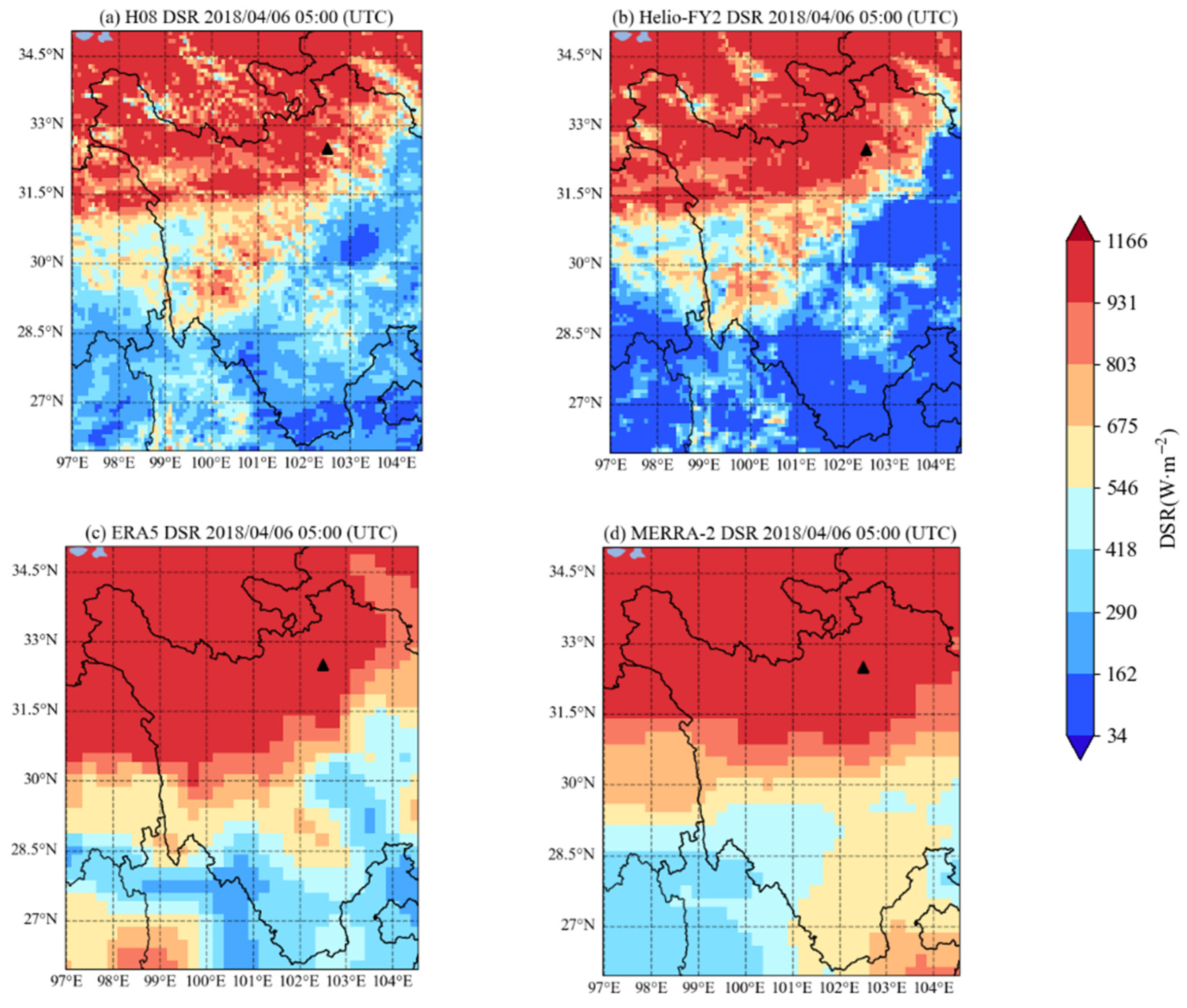
3.1. Validation of Gridded DSR Product

After applying the data quality control of Laiti et al. [53], the hourly DSR from Hongyuan is used to evaluate the original satellite observations and reanalysis datasets, with validation results shown in Figure 3. The ground-based hourly annual DSR in the WSP is 500.85 W/m², with RMSEs (nRMSEs) for the four products (H08, Helio-FY2, ERA5, and MERRA-2) of 203.85 W/m² (40.70%), 210.92 W/m² (42.11%), 245.28 W/m² (48.97%), and 235.69 W/m² (47.06%), respectively. The H08 and Helio-FY2 hourly annual DSRs are underestimated, with biases of −53.76 W/m² and −60.00 W/m², respectively, while the ERA5 and MERRA-2 show overestimation, with biases of 27.00 W/m² and 39.56 W/m², respectively. In general, the H08 DSR demonstrates the highest accuracy among the four products, with the lowest RMSE (203.85 W/m²) and the highest R² (0.58), followed by Helio-FY2; satellite products are better correlated than reanalysis products with ground-based observations. The nRMSEs in this study are consistent with those previously reported in the literature (39.08% in Du et al. [54] and 54.30% in Wang and Wang [55]), indicating that the RMSE in the WSP performs poorly in the gridded products.

Figure 4 illustrates the annual temporal variation in DSR bias between four products and the ground-based observations. The analysis reveals distinct seasonal patterns in estimation errors across different data sources. Satellite-derived DSR exhibits a pronounced negative bias during spring (March–May), while MERRA-2 demonstrates systematic overestimation in summer (June–August). All four products show relatively reduced biases during autumn (September–November) and winter (December–February). This phenomenon may be due to the enrichment of aerosols in the WSP during the spring and the frequent occurrence of cloud activity due to the summer monsoon [56]. In the spring, the enrichment of aerosols may lead to an increased retrieval error of aerosol optical depth (AOD), which in turn causes errors in the retrieval of DSR [57]. Boilley and Wald [58] proved that reanalysis often mistakes cloudy conditions as clear skies, leading to an overestimation of DSR and cloudiness in MERRA-2. This issue is particularly pronounced during periods of frequent cloud activity, which increases the DSR estimation errors in summer. These findings underscore the necessity of site adaptation to address these biases and enhance the accuracy of DSR estimation across different seasons.

3.2. Model Validation

The hourly PSA results are validated by the 16% ground-based DSRs, as shown in

Table 3. The performance of the 12 probabilistic site adaptation (PSA) methods; best results are in bold.

Methods		BIAS (W/m2)	RMSE (W/m2)	nRMSE (%)	CRPS (W/m2)
Benchmarking	BCLR	−7.25	180.79	37.96	100.25
	BCQM	−12.32	194.12	40.76	104.63
	SMA	−19.64	169.68	35.62	91.11
Stand-alone	EMOS	−33.71	169.25	35.53	91.20
	AnEn	−9.00	172.78	36.27	86.69
	QR	−21.93	166.00	34.85	85.94
	QRNN	−11.85	166.24	34.91	84.43
	QRF	−8.48	167.30	35.12	84.90
Quantile combination	AVG	−16.99	164.50	34.54	83.83
	ETQ	−17.22	164.33	34.50	83.49
	MED	−17.46	163.97	34.43	83.44
	ITQ	−16.88	164.82	34.61	84.06

. The RMSEs range from 169.68 W/m² to 194.12 W/m² over the three benchmarking methods, 166.00 W/m² to 172.78 W/m² over the five stand-alone methods, and 163.97 W/m² to 164.82 W/m² over the four quantile combination methods. Among the three benchmarking methods, the SMA has the lowest RMSE (nRMSE) of 169.68 W/m² (35.62%), while the BCQM has the highest RMSE (nRMSE) of 194.12 W/m² (40.76%); the large difference in benchmarking methods may be due to the different parametric distributions they follow. Among the stand-alone methods, the three non-parametric methods (QR, QRNN and QRF) outperform the conventional parametric methods (EMOS and AnEn) in terms of errors; the QR has the lowest RMSE (nRMSE) of 166.00 W/m² (34.85%). The quantile combination methods outperform both the benchmarking and stand-alone methods, with their RMSEs showing minimal variation among them. Among the 12 PSA methods, the MED demonstrates the highest accuracy, with the lowest RMSE of 163.97 W/m². In contrast, the BCQM has the worst performance with an RMSE of 194.12 W/m².

The CRPS is used here to simultaneously evaluate the calibration and sharpness of probabilistic forecasting methods. The CRPS values are summarized in Table 3. Among the benchmarking methods, the SMA achieves the lowest CRPS of 91.11 W/m²; the stand-alone methods achieve their best performance with the QRNN, which records the lowest CRPS of 84.43 W/m²; among all methods, the MED in the quantile combination methods exhibits the lowest CRPS of 83.44 W/m². It is also found that all quantile combination methods outperform the benchmarking methods and stand-alone methods, with MED being the overall best method. Additionally, the non-parametric methods, including QR, QRNN, QRF, AVG, ETQ, MED, and ITQ, demonstrate better prediction accuracy compared to parametric methods.

Using Kendall’s tau test [59], the 12 PSA methods are found to be statistically significant with tau values greater than 0.6 and p-values less than 0.01. The BIAS may exhibit cancelation effects between positive and negative deviations, and the RMSE and CRPS are prioritized as the primary accuracy metrics for ranking. A weighted scoring system is applied, assigning relative importance weights of 0.2 to BIAS, 0.4 to RMSE, and 0.4 to CRPS. After normalization and weighted summation, the methods are ranked comprehensively. Based on this evaluation framework, the MED method is identified as the optimal approach. Compared to the results of Yang and Gueymard [9] conducted in Europe and America, the RMSE and CRPS values of this research are higher. This discrepancy is probably due to the low accuracies of the reanalysis dataset in Asia. For instance, the monthly RMSEs of the ERA5 and MERRA-2 are 21.95 W/m² and 29.11 W/m² in Europe, whereas these values are 34.06 W/m² and 42.37 W/m² in Asia, respectively [18]. Furthermore, the MED is identified as the optimal in this study, whereas the QRF showed the best performance in the research of Yang and Gueymard [9]. The MED selects the median quantile as the result among the five stand-alone methods, which makes it more robust than the QRF [60]. Therefore, when the data contains more noise (i.e., lower accuracy), more robust methods, such as the MED, are required [61].

For the three benchmarking methods, the BCLR is suitable for predicting continuous variables with linear relationships, but may cause data overfitting when dealing with nonlinear correlations [38]; BCQM effectively corrects biases; however, due to its deterministic quantile mapping, it may result in spatial dependencies between adjacent locations in the corrected data that do not match actual conditions [39]; SMA is simple but has poor adaptability. Among the five stand-alone methods, EMOS is an easy-to-implement post-processing technique that addresses both forecast bias and under-dispersion while accounting for the spread-skill relationship [40]. However, it assumes that forecast errors follow a Gaussian distribution, which limits its applicability. AnEn improves accuracy by searching for and using historically similar weather patterns, but it requires extensive training data [41]. The three QR-based non-parametric methods perform well, especially when dealing with data with significant variance and multi-source data, although their computational complexity is higher than other parametric methods. Specifically, QR is suitable for linear or near-linear relationships with heterogeneous data [47]; QRF is ideal for in nonlinear modeling [49]; QRNN can handle large datasets with complex nonlinear relationships [48]. Finally, the four quantile combination methods can enhance the robustness of the correction data [61] by combining the quantiles of the five stand-alone methods.

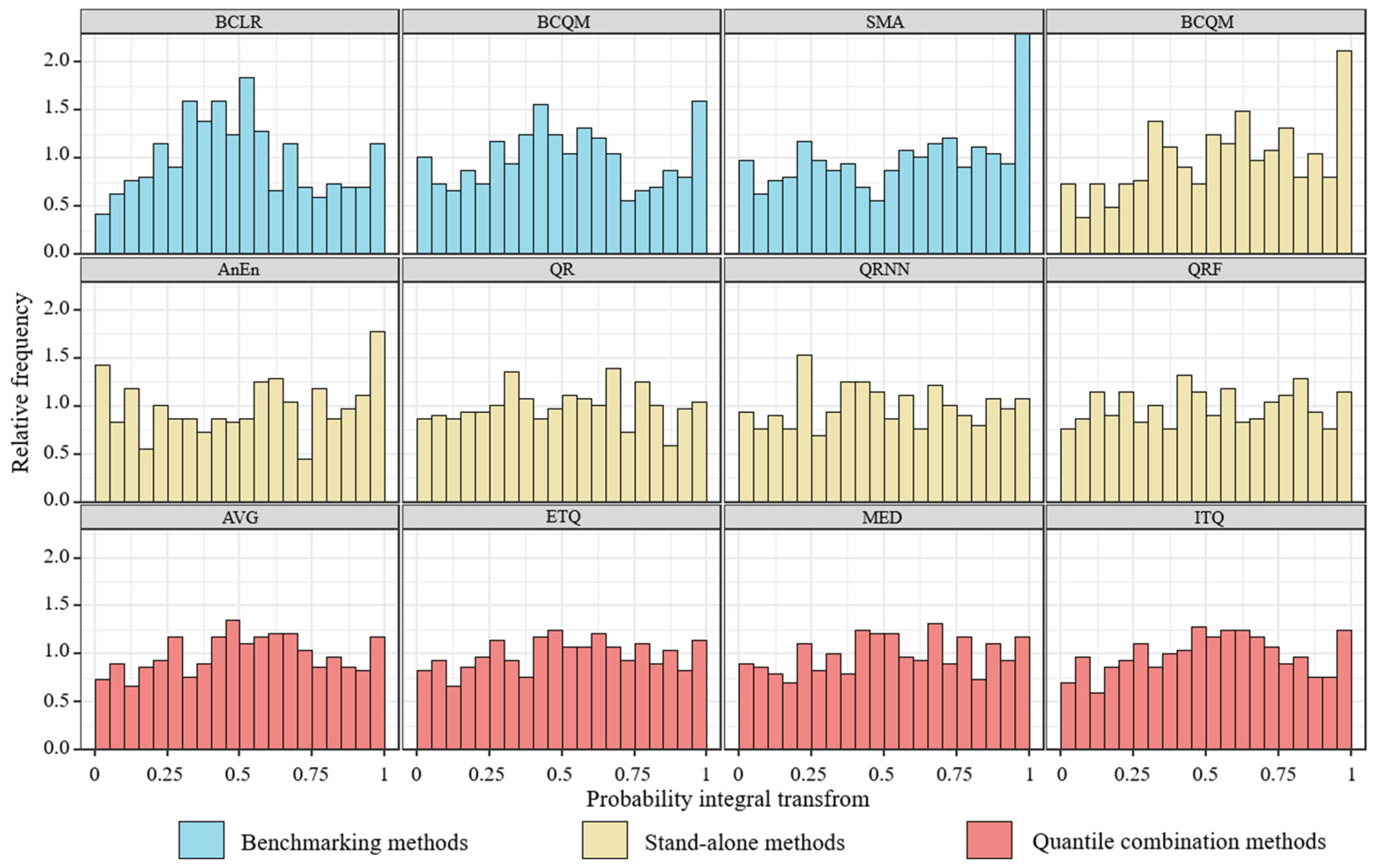
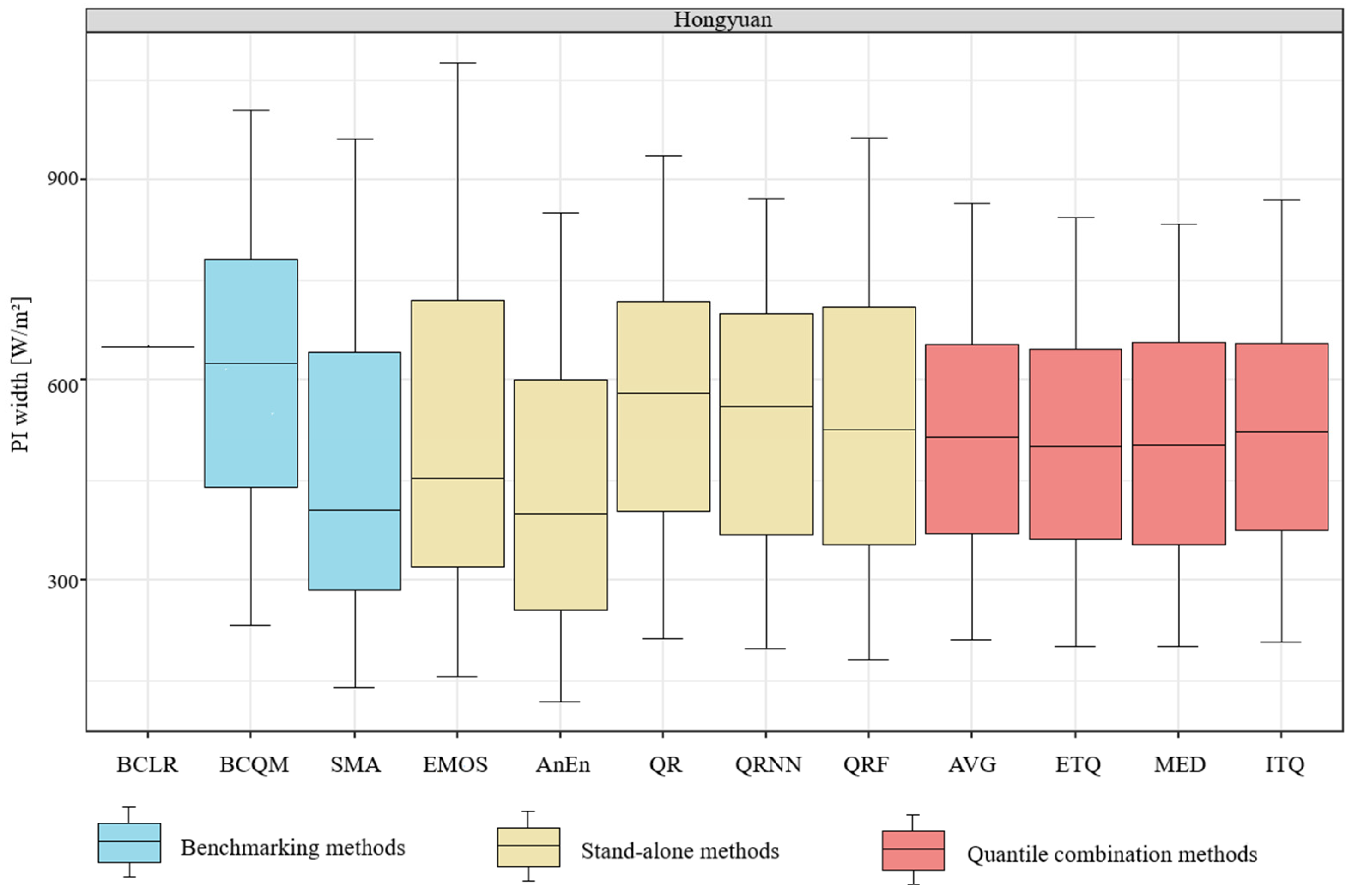
3.3. Probabilistic Forecasting Performance

To evaluate the quality of the probabilistic radiation time series forecast, the probability integral transform (PIT) histogram (Figure 5) and sharpness diagrams (Figure 6) are provided with the data from the 16% validation dataset.

As suggested by Gneiting et al. [48], the first step of an evaluation framework is to analyze the calibration of the probabilistic forecasting. Figure 5 shows the PIT histogram of the 12 PSA methods for the site. For calibrated prediction, a PIT histogram should be uniform [9]. The PIT histogram of the BCLR and BCQM exhibits an inverse-U-shape, indicating that the predictions are under-confident; put differently, the prediction distributions tend to be over-dispersed; the PIT diagram of BCLR shows a high relative frequency for the probability interval between 0.3 and 0.6; BCQM shows a high relative frequency particularly for the probability interval ranging from 0.35 to 0.6 and for the probability interval between 0.95 and 1. The PIT histogram for SMA, EMOS and AnEn tends to indicate that these methods are not calibrated, i.e., the predictive distributions tend to be under-dispersed; SMA and EMOS have a high relative frequency in a specific probability interval (0.95 to 1); AnEn shows a high relative frequency particularly for probability interval ranging from 0 to 0.05 and for probability interval between 0.95 and 1. QRNN is not calibrated at the probability interval of 0.2–0.25. The other methods show relatively uniform PIT histograms, and can be considered as calibrated.

Figure 6 shows the sharpness diagrams for each PSA method, highlighting the concentration and uncertainty of their prediction distributions. The sharpness diagram shows the distribution of the prediction interval (PI) width. In this study, the central 95% PI is used, and the PI width is the difference between the upper and lower bounds of the 95% PI. The aim of probabilistic forecasting is to maximize the sharpness of the prediction distribution [47]. The PI widths should be as short as possible, provided that the empirical coverage is at the nominal level [48]. The sharpness diagram of BCLR forms a straight line because the linear regression corrected data have similar prediction variances. This indicates that the BCLR does not distinguish between different prediction situations, resulting in a lack of discrimination. The BCQM shows a higher median (>600 W/m²), and the SMA exhibits a lower median (<450 W/m²), suggesting differences in their prediction tendencies.

Among the stand-alone methods, EMOS has the widest PIs, ranging from about 150 W/m² to 1050 W/m², reflecting greater uncertainty, followed by the QRF, AnEn, QR, and QRNN. The median of the AnEn is lower (<450 W/m²). The medians of the three quantile regression methods show closely aligned medians, suggesting similarities in their prediction tendencies. The prediction distributions issued by QR and QRNN appear to be higher in sharpness with narrower PIs compared to their peers, suggesting that the two methods reduce prediction uncertainty.

The four quantile combination methods have consistently narrow PIs, with whiskers ranging from a maximum value of less than 900 W/m² to a minimum value greater than 150 W/m², suggesting that these methods effectively reduce prediction uncertainty. The quantile combination methods rank among the best for all of the validation steps, performing better than the others. In Figure 6, the MED agrees with Table 3, showing the best results.

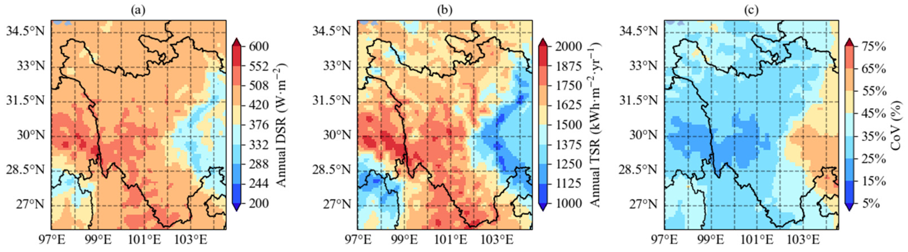
3.4. Solar Resource Analysis

According to the model validation, the best performing MED is selected for regional application, and a standardized DSR dataset is developed in the WSP. Figure 7 shows the spatial variation characteristics of the annual DSR, TSR, and CoV of solar radiation estimated by the optimal dataset with a resolution of 0.05° × 0.05° in the WSP in 2018.

The annual DSR in the WSP is 455.41 W/m², with a maximum value of 565.04 W/m² and a minimum value of 298.88 W/m². The annual TSR generally exceeds 1200 kWh/m²/yr over the WSP, with the region of the southwest reaching extremely high values ranging from 1700 to 2000 kWh/m²/yr, and the mean TSR is 1593.10 kWh/m²/yr. For the variability of solar radiation, the mean CoV is 36.07%. High CoVs (>45%) are concentrated between 102°E and 104.43°E, while low CoVs (<25%) are concentrated between 28.50–31.5°N and 97–101°E, as shown in Figure 7c. Figure 8 shows the relationship between TSR and CoV, which presents a negative correlation. For the western part of the WSP, it can conclude that the annual DSR is higher than 420 W/m², the annual TSR is higher than 1500 kWh/m²/yr, and the CoV is lower than 45%. In other words, the region with richer solar energy is accompanied by lower variability. Due to power transmission constraints, these areas, located between 97°E and 102°E in the WSP, are suitable for the deployment of PV power generation systems. The availability of accurately predicted DSR is essential for the efficient and rational utilization of solar resources and the further development of the PV industry.

4. Discussion

In this study, data from a specific site (i.e., a single grid point) are used to evaluate the optimal method, which is then applied to the WSP. The selected validation site, Hongyuan, is situated in the northeastern part of the WSP, within the upper-middle reaches of the Yellow River Basin. The vegetation distribution at this site, dominated by alpine meadows and shrublands, is broadly consistent with the predominant ecosystems across the WSP, suggesting that the site is relatively representative of the region despite its northeastern location. However, subtle climatic variations or topographic effects may still lead to prediction errors when extrapolating the results to the entire WSP.

In addition, two satellite products (Helio-FY2 and H08) and two reanalysis products (ERA5 and MERRA-2) are used in this study. The two satellites employ infrared and visible spectral channels to detect clouds, but their coarse spatial resolution (5 km) may limit the accuracy in capturing thin clouds. Meanwhile, ERA5 and MERRA-2 use cloud parameterization schemes integrated with atmospheric models, which rely on assimilated meteorological data but may misestimate cloud–aerosol interactions. To improve the accuracy of the PSA methods, future research should use data from a wider variety of sources, including higher-resolution satellite observations and ensemble reanalysis systems to better resolve cloud dynamics and radiation effects.

This study uses 1-year DSR data (spanning four seasons) to train and validate the feasibility of PSA methods with some degree level of representativeness. While this time frame captures seasonal variability, it cannot account for interannual climate change or long-term trends. It is suggested that future studies use longer time series data to conduct more thorough analyses of how climate patterns affect changes in solar radiation. Furthermore, the application of PSA methods for validation in different geographical and climatic environments will help to guide the rational use of solar energy resources under different environmental constraints.

5. Conclusions

In this study, twelve PSA methods are used to validate and predict the hourly DSR in the WSP, including three benchmarking methods, five parametric and non-parametric stand-alone methods, and four quantile combination methods. Ground-based observations are used to adapt the predictions from two satellite products and two reanalysis products. Furthermore, by comparing the PSA methods, this study develops a high-accuracy solar radiation dataset for the WSP. The main conclusions of this study are as follows:

(1)

The validation results show that satellite products (H08 and Helio-FY2) underestimate the hourly DSR, while reanalysis products (ERA5 and MERRA-2) overestimate it. All four datasets exhibit high RMSE (>200 W/m²).

(2)

Compared to the four products, all PSA methods show lower RMSEs. The quantile combination methods perform best, with each method achieving a lower RMSE (<165 W/m²) and CRPS (<85 W/m²). The MED had the lowest RMSE (nRMSE) of 163.97 W/m² (34.43%) and CRPS of 83.40 W/m².

(3)

The optimal dataset is developed using the MED method, with the spatial resolution of 0.05° × 0.05° and temporal resolution of 1 h. The mean DSR and TSR in the WSP are 455.41 W/m² and 1593.10 kWh/m²/yr, and there is a negative correlation between TSR and CoV. In other words, the WSP exhibits a high annual TSR and low radiation variability, indicating that the solar resources have significant potential for utilization.

Among the 12 methods used in this study, the benchmarking methods have strict assumptions about data distribution (e.g., linear relationships and quantile mapping), which makes their stability heavily dependent on the quality of the input data and prone to overfitting [38,39]. The two stand-alone parametric methods, mitigate input bias and improve dispersion by using probabilistic distribution assumptions (Gaussian distribution) and historical analog search, but remain constrained by their inherent distribution hypotheses [40,41]. The QR-based non-parametric methods are flexible in capturing nonlinear features and demonstrate strong adaptability, especially when dealing with complex variance and multi-source data fusion [47,48,49]. Quantile combination methods further enhance robustness by integrating outputs from stand-alone methods [61]. Although their computational complexity increases with sample size, they provide optimal accuracy and performance under sufficient data conditions, outperforming other methods in balancing precision and generalizability.

References

1. Nielsen, A.H.; Iosifidis, A.; Karstoft, H. IrradianceNet: Spatiotemporal deep learning model for satellite-derived solar irradiance short-term forecasting. Sol. Energy 2021, 228, 659–669. [Google Scholar] [CrossRef]
2. Zhang, J.; Zhao, L.; Deng, S.; Xu, W.; Zhang, Y. A critical review of the models used to estimate solar radiation. Renew. Sustain. Energy Rev. 2017, 70, 314–329. [Google Scholar] [CrossRef]
3. Huang, G.; Li, Z.; Li, X.; Liang, S.; Yang, K.; Wang, D.; Zhang, Y. Estimating surface solar irradiance from satellites: Past, present, and future perspectives. Remote Sens. Environ. 2019, 233, 111371–111386. [Google Scholar] [CrossRef]
4. Yang, D.; Wang, W.; Xia, X.A. A concise overview on solar resource assessment and forecasting. Adv. Atmos. Sci. 2022, 39, 1239–1251. [Google Scholar] [CrossRef]
5. Huang, C.; Shi, H.; Yang, D.; Gao, L.; Zhang, P.; Fu, D.; Xia, X.; Chen, Q.; Yuan, Y.; Liu, M.; et al. Retrieval of sub-kilometer resolution solar irradiance from Fengyun-4A satellite using a region-adapted Heliosat-2 method. Sol. Energy 2023, 264, 112038. [Google Scholar] [CrossRef]
6. Choi, Y.; Suh, J.; Kim, S.M. GIS-based solar radiation mapping, site evaluation, and potential assessment: A review. Appl. Sci. 2019, 9, 1960. [Google Scholar] [CrossRef]
7. Xia, X.A.; Wang, P.C.; Chen, H.B.; Liang, F. Analysis of downwelling surface solar radiation in China from National Centers for Environmental Prediction reanalysis, satellite estimates, and surface observations. J. Geophys. Res. Atmos. 2006, 111, D09103. [Google Scholar] [CrossRef]
8. Liang, S.; Wang, D.; He, T.; Yu, Y. Remote sensing of earth’s energy budget: Synthesis and review. Int. J. Digit. Earth 2019, 12, 737–780. [Google Scholar] [CrossRef]
9. Yang, D.; Gueymard, C.A. Probabilistic post-processing of gridded atmospheric variables and its application to site adaptation of shortwave solar radiation. Sol. Energy 2021, 225, 427–443. [Google Scholar] [CrossRef]
10. Letu, H.; Nakajima, T.Y.; Wang, T.; Shang, H.; Ma, R.; Yang, K.; Baran, A.J.; Riedi, J.; Ishimoto, H.; Yoshida, M.; et al. A new benchmark for surface radiation products over the East Asia-Pacific region retrieved from the Himawari-8/AHI next-generation geostationary satellite. Bull. Am. Meteorol. Soc. 2022, 103, E873–E888. [Google Scholar] [CrossRef]
11. Xian, D.; Zhang, P.; Gao, L.; Sun, R.; Zhang, H.; Jia, X. Fengyun meteorological satellite products for earth system science applications. Adv. Atmos. Sci. 2021, 38, 1267–1284. [Google Scholar] [CrossRef]
12. Trenberth, K.E.; Olson, J.G. An evaluation and intercomparison of global analyses from the National Meteorological Center and the European Centre for Medium Range Weather Forecasts. Bull. Am. Meteorol. Soc. 1988, 69, 1047–1057. [Google Scholar] [CrossRef]
13. Yang, D.; Bright, J.M. Worldwide validation of 8 satellite-derived and reanalysis solar radiation products: A preliminary evaluation and overall metrics for hourly data over 27 years. Sol. Energy 2020, 210, 3–19. [Google Scholar] [CrossRef]
14. Dee, D.P.; Uppala, S.M.; Simmons, A.J.; Berrisford, P.; Poli, P.; Kobayashi, S.; Andrae, U.; Balmaseda, M.A.; Balsamo, G.; Bauer, P.; et al. The ERAInterim reanalysis: Configuration and performance of the data assimilation system. Q. J. R. Meteorol. Soc. 2011, 137, 553–597. [Google Scholar] [CrossRef]
15. Cao, Q.; Liu, Y.; Sun, X.; Yang, L. Country-level evaluation of solar radiation data sets using ground measurements in China. Energy 2022, 241, 122938. [Google Scholar] [CrossRef]
16. Bright, J.M. Solcast: Validation of a satellite-derived solar irradiance dataset. Sol. Energy 2019, 189, 435–449. [Google Scholar] [CrossRef]
17. Babar, B.; Graversen, R.; Boström, T. Solar radiation estimation at high latitudes: Assessment of the CMSAF databases, ASR and ERA5. Sol. Energy 2019, 182, 397–411. [Google Scholar] [CrossRef]
18. Zhang, X.; Liang, S.; Wang, G.; Yao, Y.; Jiang, B.; Cheng, J. Evaluation of the reanalysis surface incident shortwave radiation products from NCEP, ECMWF, GSFC, and JMA using satellite and surface observations. Remote Sens. 2016, 8, 225. [Google Scholar] [CrossRef]
19. Qian, P.Z.; Wu, C.J. Bayesian hierarchical modeling for integrating low-accuracy and high-accuracy experiments. Technometrics 2008, 50, 192–204. [Google Scholar] [CrossRef]
20. Xiong, S.; Qian, P.Z.; Wu, C.J. Sequential design and analysis of high-accuracy and low-accuracy computer codes. Technometrics 2013, 55, 37–46. [Google Scholar] [CrossRef]
21. Yang, D.; Gueymard, C.A. Producing high-quality solar resource maps by integrating high-and low-accuracy measurements using Gaussian processes. Renew. Sustain. Energy Rev. 2019, 113, 109260. [Google Scholar] [CrossRef]
22. Weiss, A.; Hays, C.J. Simulation of daily solar irradiance. Agric. For. Meteorol. 2004, 123, 187–199. [Google Scholar] [CrossRef]
23. Abraha, M.G.; Savage, M.J. Comparison of estimates of daily solar radiation from air temperature range for application in crop simulations. Agric. For. Meteorol. 2008, 148, 401–416. [Google Scholar] [CrossRef]
24. Liu, J.; Pan, T.; Chen, D.; Zhou, X.; Yu, Q.; Flerchinger, G.N.; Shen, Y. An improved Ångström-type model for estimating solar radiation over the Tibetan Plateau. Energies 2017, 10, 892. [Google Scholar] [CrossRef]
25. Suri, M.; Cebecauer, T. Requirements and standards for bankable DNI data products in CSP projects. In Proceedings of the SolarPACES Conference, Granada, Spain, 20−23 September 2011. [Google Scholar]
26. Polo, J.; Wilbert, S.; Ruiz-Arias, J.; Meyer, R.; Gueymard, C.; Súri, M.; Martín, L.; Mieslinger, T.; Blanc, P.; Grant, I.; et al. Preliminary survey on site-adaptation techniques for satellite derived and reanalysis solar radiation datasets. Sol. Energy 2016, 132, 25–37. [Google Scholar] [CrossRef]
27. Polo, J.; Fernandez-Peruchena, C.; Salamalikis, V.; Mazorra-Aguiar, L.; Turpin, M.; Martin-Pomares, L.; Kazantzidis, A.; Blanc, P.; Remund, J. Benchmarking on improvement and site-adaptation techniques for modeled solar radiation datasets. Sol. Energy 2020, 201, 469–479. [Google Scholar] [CrossRef]
28. Yang, D.; Liu, L. Solar project financing, bankability, and resource assessment. In Sustainable Energy Solutions for Remote Areas in the Tropics; Springer: Cham, Switzerland, 2020; pp. 179–211. [Google Scholar] [CrossRef]
29. Feng, Q.; Niu, B.; Ren, Y.; Su, S.; Wang, J.; Shi, H.; Yang, J.; Han, M. A 10-m national-scale map of ground-mounted photovoltaic power stations in China of 2020. Sci. Data 2024, 11, 198. [Google Scholar] [CrossRef]
30. Hu, Y.; Huang, W.; Wang, J.; Chen, S.; Zhang, J. Current status, challenges, and perspectives of Sichuan’s renewable energy development in Southwest China. Renew. Sustain. Energy Rev. 2016, 57, 1373–1385. [Google Scholar] [CrossRef]
31. Zhang, J.; Liu, B.; Ren, S.; Han, W.; Ding, Y.; Peng, S. A 4 km daily gridded meteorological dataset for China from 2000 to 2020. Sci. Data 2024, 11, 1230. [Google Scholar] [CrossRef]
32. Tang, L.; Liu, Y.; Pan, Y.; Ren, Y.; Yao, L.; Li, X. Optimizing solar photovoltaic plant siting in Liangshan Prefecture, China: A policy-integrated, multi-criteria spatial planning framework. Sol. Energy 2024, 283, 113012. [Google Scholar] [CrossRef]
33. Bessho, K.; Date, K.; Hayashi, M.; Ikeda, A.; Imai, T.; Inoue, H.; Yoshida, R. An introduction to Himawari-8/9—Japan’s new-generation geostationary meteorological satellites. J. Meteorol. Soc. Jpn. 2016, 94, 151–183. [Google Scholar] [CrossRef]
34. Urraca, R.; Huld, T.; Gracia-Amillo, A.; Martinez-de-Pison, F.J.; Kaspar, F.; Sanz-Garcia, A. Evaluation of global horizontal irradiance estimates from ERA5 and COSMO-REA6 reanalyses using ground and satellite-based data. Sol. Energy 2018, 164, 339–354. [Google Scholar] [CrossRef]
35. Gelaro, R.; McCarty, W.; Suárez, M.J.; Todling, R.; Molod, A.; Takacs, L.; Randles, C.A.; Darmenov, A.; Bosilovich, M.G.; Reichle, R.; et al. The modern-era retrospective analysis for research and applications, version 2 (MERRA-2). J. Clim. 2017, 30, 5419–5454. [Google Scholar] [CrossRef]
36. Wang, K.; Ma, Q.; Li, Z.; Wang, J. Decadal variability of surface incident solar radiation over China: Observations, satellite retrievals, and reanalyses. J. Geophys. Res. Atmos. 2015, 120, 6500–6514. [Google Scholar] [CrossRef]
37. Feng, F.; Wang, K. Merging ground-based sunshine duration observations with satellite cloud and aerosol retrievals to produce high-resolution long-term surface solar radiation over China. Earth Syst. Sci. Data 2021, 13, 907–922. [Google Scholar] [CrossRef]
38. Maulud, D.; Abdulazeez, A.M. A review on linear regression comprehensive in machine learning. J. Appl. Sci. Technol. Trends 2020, 1, 140–147. [Google Scholar] [CrossRef]
39. Maraun, D. Bias correction, quantile mapping, and downscaling: Revisiting the inflation issue. J. Clim. 2013, 26, 2137–2143. [Google Scholar] [CrossRef]
40. Wasserman, L. All of nonparametric statistics. Technometrics 2007, 49, 103. [Google Scholar] [CrossRef]
41. Yang, D.; Alessandrini, S. An ultra-fast way of searching weather analogs for renewable energy forecasting. Sol. Energy 2019, 185, 255–261. [Google Scholar] [CrossRef]
42. Yang, D.; van der Meer, D.; Munkhammar, J. Probabilistic solar forecasting benchmarks on a standardized dataset at Folsom, California. Sol. Energy 2020, 206, 628–639. [Google Scholar] [CrossRef]
43. Junk, C.; Delle Monache, L.; Alessandrini, S.; Cervone, G.; Von Bremen, L. Predictor-weighting strategies for probabilistic wind power forecasting with an analog ensemble. Meteorol. Z 2015, 24, 361–379. [Google Scholar] [CrossRef]
44. Junk, C.; Delle Monache, L.; Alessandrini, S. Analog-based ensemble model output statistics. Mon. Weather Rev. 2015, 143, 2909–2917. [Google Scholar] [CrossRef]
45. Meinshausen, N.; Ridgeway, G. Quantile regression forests. J. Mach. Learn. Res. 2006, 7, 983–999. [Google Scholar]
46. Koenker, R. Quantile regression. In Econometric Society Monographs; Cambridge University Press: Cambridge, UK, 2005. [Google Scholar] [CrossRef]
47. Koenker, R.; Bassett, G. Regression quantiles. Econom. J. Econom. Soc. 1978, 46, 33–50. [Google Scholar] [CrossRef]
48. Cannon, A.J. Quantile regression neural networks: Implementation in R and application to precipitation downscaling. Comput. Geosci. 2011, 37, 1277–1284. [Google Scholar] [CrossRef]
49. Breiman, L. Random forests. Mach. Learn. 2001, 45, 5–32. [Google Scholar] [CrossRef]
50. Gneiting, T.; Katzfuss, M. Probabilistic forecasting. Annu. Rev. Stat. Its Appl. 2014, 1, 125–151. [Google Scholar] [CrossRef]
51. Gneiting, T.; Balabdaoui, F.; Raftery, A.E. Probabilistic forecasts, calibration and sharpness. J. R. Stat. Soc. Ser. B Stat. Methodol. 2007, 69, 243–268. [Google Scholar] [CrossRef]
52. Gneiting, T.; Raftery, A.E. Strictly proper scoring rules, prediction, and estimation. J. Am. Stat. Assoc. 2007, 102, 359–378. [Google Scholar] [CrossRef]
53. Laiti, L.; Andreis, D.; Zottele, F.; Giovannini, L.; Panziera, L.; Toller, G.; Zardi, D. A solar atlas for the Trentino region in the Alps: Quality control of surface radiation data. Energy Procedia 2014, 59, 336–343. [Google Scholar] [CrossRef]
54. Du, Y.; Shi, H.; Zhang, J.; Xia, X.; Yao, Z.; Fu, D.; Bo, H.; Huang, C. Evaluation of MERRA-2 hourly surface solar radiation across China. Sol. Energy 2022, 234, 103–110. [Google Scholar] [CrossRef]
55. Wang, H.; Wang, Y. Evaluation of the Accuracy and Trend Consistency of Hourly Surface Solar Radiation Datasets of ERA5, MERRA-2, SARAH-E, CERES, and Solcast over China. Remote Sens. 2025, 17, 1317. [Google Scholar] [CrossRef]
56. Li, T.; Xin, X.; Zhang, H.; Yu, S.; Li, L.; Ye, Z.; Liu, Q.; Cai, H. Evaluation of Six Data Products of Surface Downward Shortwave Radiation in Tibetan Plateau Region. Remote Sens. 2024, 16, 791. [Google Scholar] [CrossRef]
57. Filonchyk, M.; Yan, H.; Zhang, Z.; Yang, S.; Li, W.; Li, Y. Combined use of satellite and surface observations to study aerosol optical depth in different regions of China. Sci. Rep. 2019, 9, 6174. [Google Scholar] [CrossRef]
58. Boilley, A.; Wald, L. Comparison between meteorological re-analyses from ERA-Interim and MERRA and measurements of daily solar irradiation at surface. Renew. Energy 2015, 75, 135–143. [Google Scholar] [CrossRef]
59. Kendall, M.G. A new measure of rank correlation. Biometrika 1938, 30, 81–93. [Google Scholar] [CrossRef]
60. Lecué, G.; Lerasle, M. Robust machine learning by median-of-means: Theory and practice. Ann. Statist. 2020, 48, 906–931. [Google Scholar] [CrossRef]
61. Wang, X.; Fang, Z. Robust recursive estimation for the errors-in-variables nonlinear systems with impulsive noise. Sci. Rep. 2025, 15, 6031. [Google Scholar] [CrossRef]
Figure 1. Topographical map of the research area.
Remotesensing 17 01720 g001
Figure 2. The spatial distributions of hourly downward shortwave radiation (DSR) from (ad), namely Himawari-8 (H08), Helio-FY2, ERA5, and MERRA-2, respectively, at 5:00 UTC on 6 April 2018 within the study area; the black triangle represents the location of Hongyuan.
Remotesensing 17 01720 g002
Figure 3. Validation results of hourly satellite and reanalysis products with ground-based measurements in 2018. (a) H08; (b) Helio-FY2; (c) ERA5; (d) MERRA-2. The red lines indicate the 1:1 line.
Remotesensing 17 01720 g003
Figure 4. The bias between the daily DSR of the ground-based observations and (a) satellite products and (b) reanalysis products in 2018; the shadow is the data with an error of less than 50 W/m2.
Remotesensing 17 01720 g004
Figure 5. Probability integral transform diagrams of the 12 PSA methods.
Remotesensing 17 01720 g005
Figure 6. Sharpness diagrams of the 12 PSA methods.
Remotesensing 17 01720 g006
Figure 7. (a) Annual DSR estimated from the hourly median ensemble (MED) dataset. (b) Annual total solar radiation (TSR) obtained from the hourly MED dataset. (c) Coefficient of variation (CoV) estimated from the daily MED dataset.
Remotesensing 17 01720 g007
Figure 8. The relationship between the TSR and the CoV, where the red line indicates linear regression fits.
Remotesensing 17 01720 g008