Temporal and Spatial Distribution of 2022–2023 River Murray Major Flood Sediment Plume

Abstract

This study examined a sediment plume from Australia’s largest river, The River Murray, which was produced during a major flood event in 2022–2023. This flood resulted from successive La Niña events, causing high rainfall across the Murray–Darling Basin and ultimately leading to a significant riverine flow through South Australia. The flood was characterised by a significant increase in riverine discharge rates, reaching a peak of 1305 m³/s through the Lower Lakes barrage system from November 2022 to February 2023. The water quality anomaly within the coastal region (<~150 km offshore) was effectively quantified and mapped utilising the diffuse attenuation coefficient at 490 nm (Kd490) from products derived from MODIS Aqua Ocean Color satellite imagery. The sediment plume expanded and intensified alongside the increased riverine discharge rates, which reached a maximum spatial extent of 13,681 km². The plume typically pooled near the river’s mouth within the northern corner of Long Bay, before migrating persistently westward around the Fleurieu Peninsula through Backstairs Passage into Gulf St Vincent, occasionally exhibiting brief eastward migration periods. The plume gradually subsided by late March 2023, several weeks after riverine discharge rates returned to pre-flood levels, indicating a lag in attenuation. The assessment of the relationship and accuracy between the Kd490 product and the surface-most in situ turbidity, measured using conductivity, temperature, and depth (CTD) casts, revealed a robust positive linear correlation (R² = 0.85) during a period of high riverine discharge, despite temporal and spatial discrepancies between the two datasets. The riverine discharge emerged as an important factor controlling the spatial extent and intensities of the surface sediment plume, while surface winds also exerted an influence, particularly during higher wind velocity events, as part of a broader interplay with other drivers.

1. Introduction

1.1. Sediment Plumes

Rivers transport sediments, minerals, and biological material into the sea. This riverine water, typically less saline than seawater and therefore more buoyant, often forms a distinct plume on the sea’s surface. This plume can vary from a quick dispersion to extending many kilometres into the sea, and it can be relatively thin or extend many metres vertically in the water column. As riverine waters flow seaward, the water quality changes in relation to inputs of both terrigenous and anthropogenic material [1] and mixing processes. Water quality changes relate to increases in both dissolved and suspended sediments, ranging from naturally occurring riverine bank materials to pollutant input from industries in proximity to the riverine system [2].

This riverine discharge is known as a sediment plume for as long as discharged sediments remain suspended in the water column and are in distinct contrast to surrounding coastal waters [3]. As the sediment plume ages, it spreads outward (also downward) and disperses, until it reaches a point (in distance or time) where it is fully mixed and in equilibrium with the surrounding coastal waters [4].

Sediment plumes have a range of ecological impacts on coastal and oceanic environments. While some ecological benefits, such as increased nutrient loads, can occur [5], negative impacts are often more prominent. These include the deterioration of the water quality, which can lead to the death of marine organisms and create biogeochemical imbalances, such as disruptions in nutrient cycling and altered oxygen levels [6,7,8,9]. The turbidity associated with sediment plumes also limits light penetration in the water column, affecting light-dependent ecosystems [10,11]. Prolonged high turbidity can severely reduce light availability, causing stress to marine life and potentially leading to long-term ecosystem changes [12,13]. Additionally, the resuspension of fine particles, which can result from wave action or tidal currents, may create more persistent water quality issues, further compounding ecological impacts [14]. These effects vary across plumes depending on factors such as magnitude, duration, intensity, and the specific environmental conditions in affected areas. Therefore, understanding the temporal and spatial distribution of a sediment plume is of high importance for understanding natural processes, interactions with marine ecosystems, and the various industries operating in and around the coastal zone impacted by the plume.

1.2. Sediment Plume Dynamics and Drivers

Sediment plumes spread and move in response to various environmental drivers, including riverine discharge, surface winds, ocean currents, tidal cycles, waves, and bathymetry, with their dynamics influenced by these factors as well as the plume’s density and the physical features of the coastal environment [15,16]. A complex interplay exists among these drivers as many are influenced by one another. Numerous observational and modelling studies have identified riverine discharge and surface winds as the primary drivers of surface dynamics [3,5,9,17,18,19,20,21,22,23]. Riverine discharge is the primary driver of the spatio-temporal dynamics of the plume by influencing both the volume of sediment persisting at the discharge point and the velocity of the seaward jet. Thereafter, surface winds play a significant role in modulating the plume dynamics in two ways. Local winds directly push the surface waters, altering the immediate movement and dispersion of the plume. In contrast, regional winds indirectly influence the plume by shaping larger-scale ocean currents and wave patterns, which affect the direction and strength of the plume’s spread over a broader area [24,25].

Sediment plumes can exhibit both unidirectional and multidirectional dynamics. Unidirectional dynamics involve the plume predominantly moving in a single direction, generally influenced by river discharge and prevailing currents. In contrast, multidirectional dynamics occur when the plume branches off in various directions, often due to local wind patterns, tidal forces, or interactions with coastal features. This branching can form smaller subsidiary plumes or eddies that alter sediment dispersion [17,26]. Additionally, modelling studies have suggested that the Coriolis force consistently influences plume dynamics, causing discharge to veer clockwise in the northern hemisphere and anticlockwise in the southern hemisphere [3,27].

The dynamics of sediment plumes are non-uniform due to variations in geographical features, environmental drivers, and riverine characteristics. Therefore, analysing sediment plumes on an individual basis can yield valuable insights into their regional drivers. This approach is particularly relevant for understanding the seasonality and sensitivity of individual plumes, which may occur persistently or in response to changing environmental conditions [25,28].

1.3. Remote Sensing of Sediment Plumes

The distinct difference in water quality between a sediment plume and its surrounding coastal water allows the surface plume to be visualised against the background coastal environment through satellite imagery [29]. Turbidity is a key water quality metric that indicates water clarity, which influences light scattering and absorption and can be estimated through space-borne observations [25,30,31]. While turbidity is commonly associated with suspended sediments, it is essential to recognise that dissolved compounds, such as chlorophyll-a, can also contribute to turbidity through their scattering and absorption properties [28,32,33]. As a result, turbidity may not solely reflect the presence of suspended solids but can also be influenced by dissolved substances. This distinction is important because different turbidity metrics have varying sensitivities to these components, which can affect their interpretation in sediment plume dynamics [34]. Understanding these limitations is crucial for accurately assessing water quality in complex environments.

Remote sensing has been employed extensively in the blue to red range of the electromagnetic spectrum and from a variety of sensors to derive turbidity values, allowing for the identification and tracking of sediment plumes at a surface level [9,32]. Among these, the MODIS diffuse attenuation coefficient at 490 nm (Kd490)product stands out due its global coverage, accessibility, and region-independent nature [35,36].

Kd490 estimates the rate at which light at 490 nm is attenuated with depth by analysing the ratio of blue to green wavelengths [37,38,39,40]. Given that this attenuation is influenced by particles and dissolved matter, Kd490 values often show a strong correlation with turbidity, particularly when compared against Nephelometric Turbidity Units (NTUs), which are generally measured using white light sources from the 400–680 nm range [41].

The Kd490 value is derived from established optical models and calibration coefficients, representing the sum of the bio-optical attenuation component K_bio(490) and the pure water constant of 0.0166 [35,36,42]. The processing of MODIS data to accurately retrieve the essential remote sensing reflectance data is conducted using the National Aeronautics and Space Administration’s (NASA) SeaDAS software 9.2.0, which applies atmospheric corrections optimised for ocean retrievals [43,44].

This study utilises Kd490 estimates due to the coefficient’s ease of access through NASA’s Ocean Color archive and the opportunity to assess its performance by comparing it to in situ NTU turbidity data. Kd490 has yielded great results due to its sensitivity to water quality changes, performing particularly well for high turbidity applications, making it well-suited for sediment plume studies. However, an apparent limitation of the product is the influence substrate plays on the results computed in shallow water applications, due to the penetration depth of the wavelengths [45].

The Kd490 estimate’s nuanced difference from turbidity is important to understand, with turbidity indicating the cloudiness of a liquid and Kd490 indicating the rate at which light at 490 nm is attenuated with depth (m⁻¹) [35]. The higher the value of Kd490, the shallower the attenuation depth and the lower the clarity of the water measured. For example, a Kd490 value of 0.1 L/m indicates greater water clarity than a Kd490 value of 0.5 L/m, with a reduction in light intensity by one natural log occurring within 10 and 5 m of water, respectively. At a Kd490 value of 0.1 L/m, approximately 10% of the light intensity would be reduced at 10 m, whereas at a Kd490 value of 0.5 L/m, around 60% of the light intensity would be reduced at the same depth. This illustrates how higher Kd490 values correspond to significantly reduced light penetration and clarity.

The Kd490 product allows quality-assured, cloud-free satellite imagery to be converted into robust and accurate water clarity datasets, allowing for the analysis of surface sediment plume distributions. Globally, daily MODIS imagery has been widely used to observe short-term changes in plume behaviour due to its high temporal resolution [9,15,46,47,48]. Given the absence of published sediment plume detection techniques within South Australian waters, this study applies the MODIS Aqua Kd490 product to assess its regional suitability and lay the foundation for future analyses and methodological comparisons.

This study aims to quantify the magnitude and spatio-temporal dynamics of the flood-induced surface sediment plume that persisted following a major discharge event. Specifically, we (1) utilise the Kd490 product to detect and track surface sediment plumes in South Australian coastal waters, (2) examine the correlation between riverine discharge rates and both sediment plume area and water quality levels, (3) explore the temporal and spatial distribution of the sediment plume, including the relationship between in situ turbidity data and the distance offshore, and (4) assess the correlation between remotely sensed Kd490 estimates and all available in situ turbidity data. This study is not focused on the sediment plume’s ecological impacts and sub-surface dynamics but rather on the surface temporal and spatial distributions of the plume.

2. Materials and Methods

2.1. Major River Murray Flood Event

An “exceptionally” significant flood event occurred on the River Murray between November 2022 and February 2023 [49,50,51]. This was the largest flood event in South Australia since 1956 and the third largest since records began in 1931 [52]. The River Murray flooding was the result of heavy rainfall and flood events within the broader Murray–Darling Basin (MDB) that spans more than 1 million km² across three states in eastern Australia [53]. The River Murray serves as a vital link between the MDB and the ocean as the essential outlet for the water collected within the basin. The spatial relationship between Australia, the MDB, and the River Murray is illustrated in Figure 1a.

Daily flow rates at the South Australian/Victorian (SA/VIC) border peaked at 2153 m³/s on 22 December 2022, with the travel time to the Lower Lakes estimated to take 21 days [49,51,54]. The Lower Lakes, largely represented by Lake Alexandrina, are illustrated in Figure 1b, highlighting the relationship between the Lower Lakes and the Murray Mouth. The daily flow rates calculated by the Department of Environment and Water (DEW) at the SA/VIC border are presented in Figure 2, alongside flow rate thresholds set by the DEW [55]. The time series underscores the flood event’s significance, where the dataset exceeds the “high flow” threshold consecutively from June 2023 to February 2024.

The significance of the flood event, combined with the extensive spatial reach of the MDB, indicates that the floodwaters discharged at the Murray Mouth travelled a long distance. This journey passed through a diverse range of land uses. The MDB’s high density of agricultural activity brings a heightened potential for pollutants and terrestrial materials to be carried by the floodwaters, decreasing the quality of the discharged water [15,57]. As this was the first flood of its magnitude since the 1950s, a substantial accumulation of organic material along the riverbanks is also likely to have contributed to the degradation of the water quality. The major transport of sediment, minerals, and biological materials down the River Murray resulted in a dynamic sediment plume forming in Long Bay. Significant impacts to the fisheries and tourism industries occurred along the coast for months during the summer period. These impacts are attributed to the drastic degradation of the water quality, which prevented safe recreational use and affected the export of fishery products. Adding to health concerns, the discharged flood water correlated with the mass die-off of marine species and the clear visual discolouration of coastal waters [58]. Satellite images of the resultant sediment plume show (Figure 3 and Figure 4) that these impacts spread extensively as the sediment plume itself dispersed into the greater Long Bay region.

2.2. Ocean Colour Imagery

To quantify the temporal and spatial distributions of the River Murray sediment plume across the 2022–2023 flood event, this study utilised NASA’s “Ocean Color Level-3 Standard Mapped Images” product. This imagery is captured by the MODIS sensor on the Aqua satellite, which consistently passes over the study site at approximately 1:30 PM local time each day [60]. These daily surface data are available at a resolution of 4616 m and are stored in an open-access dataset spanning from July 2002 to the present day [61].

The selection of MODIS Aqua data for this study was based on several critical factors. A significant advantage is the use of SeaDAS, which implements atmospheric correction algorithms that, while generic and applicable to various sensors, are particularly effective for ocean retrievals. Additionally, compared to other open-access satellite imagery products, MODIS Aqua offers superior radiometric and temporal resolutions.

Level 3 Ocean Color products possess only the “highest-quality” data by masking pixels that do not meet stringent quality criteria. These criteria include quality flags such as “pixel is over land”, “sunglint: reflectance exceeds threshold”, and “probable cloud or ice contamination” among others, which ensure that only the most reliable data are utilised. A comprehensive list of the criteria triggering pixel masking is available at https://oceancolor.gsfc.nasa.gov/resources/atbd/ocl2flags/ (accessed 3 May 2024), highlighting the extensive quality assurance measures associated with this product.

Although the spatial resolution of 4616 m may limit fine-scale assessments, the inclusion of pre-processed Kd490 estimates supports the selection of MODIS Aqua for this study, as the data have been successfully applied to monitor turbidity and sediment plumes in coastal environments [62,63]. Aqua’s stable sun–sensor geometry provides more consistent retrievals compared to MODIS Terra, especially in regions affected by cloud cover. Additionally, Aqua’s afternoon pass likely results in fewer cloud obstructions, facilitating the effective monitoring of the sediment plume across the flood event.

2.3. Data Processing

2.3.1. Kd490 Estimates

The outlined MODIS Aqua Kd490 estimates were downloaded from: https://oceancolor.gsfc.nasa.gov/l3/ (accessed 3 May 2024), with the data downloaded in 8-day composite periods from 4 July 2002 to 10 February 2024, capturing the entire temporal record to download date.

The “8-day”, or as referred to by NASA as “weekly”, period directs the composition of data from days 1 to 8 [64]. Due to the aggressive masking of pixels to ensure the “highest-quality” data, the daily MODIS Aqua captures are often sporadic. The 8-day composite helps create a more stable dataset by averaging high-quality observations over this period.

A reference date of 1 July 2022, was chosen to establish long-term reference datasets for Kd490, encompassing the entire MODIS data record preceding the 2022–2023 Murray River flood event. This date was chosen to exclude any flood event data, providing a robust baseline for subsequent analysis. Although there may be a temporal gap between this reference date and the onset of the flood event, the extensive archive of MODIS data effectively bridges this temporal disparity. Figure 5 illustrates the Murray River flow across 2022, highlighting the 1st of July’s position relative to the increasing flow and breaching of the DEW-defined high flow threshold.

We processed two summarised datasets to analyse the Kd490 estimates. First, we calculated Kd490 summary statistics for each pixel for data preceding 1 July 2022. We used this pre-flood as a reference period to calculate monthly summary statistics including the median (kd_p50), 5th percentile (kd_p5), and 95th percentile (kd_p95), outlining monthly Kd490 expectations.

Next, we extracted a zonal time series of summary statistics covering the Murray Mouth zone (Figure 1), both preceding the reference date (monthly) and following the reference date (“weekly”). These summary statistics include the median (zkd_p50), 5th percentile (zkd_p5), and the 95th percentile (zkd_p95), along with the number of pixels used in each calculation (nobs). The Murray Mouth zone illustrated in Figure 1 is defined as the area within 10 km of the Murray Mouth and waters less than 30 m deep. However, the accuracy of this delineation is influenced by the reliance on a single open-access bathymetric product in the region, which has a resolution of 250 m and heavily relies on interpolation between survey points [65,66].

This comprehensive framework allows for comparative analyses and anomaly detection across two different spatial contexts in the Kd490 estimates.

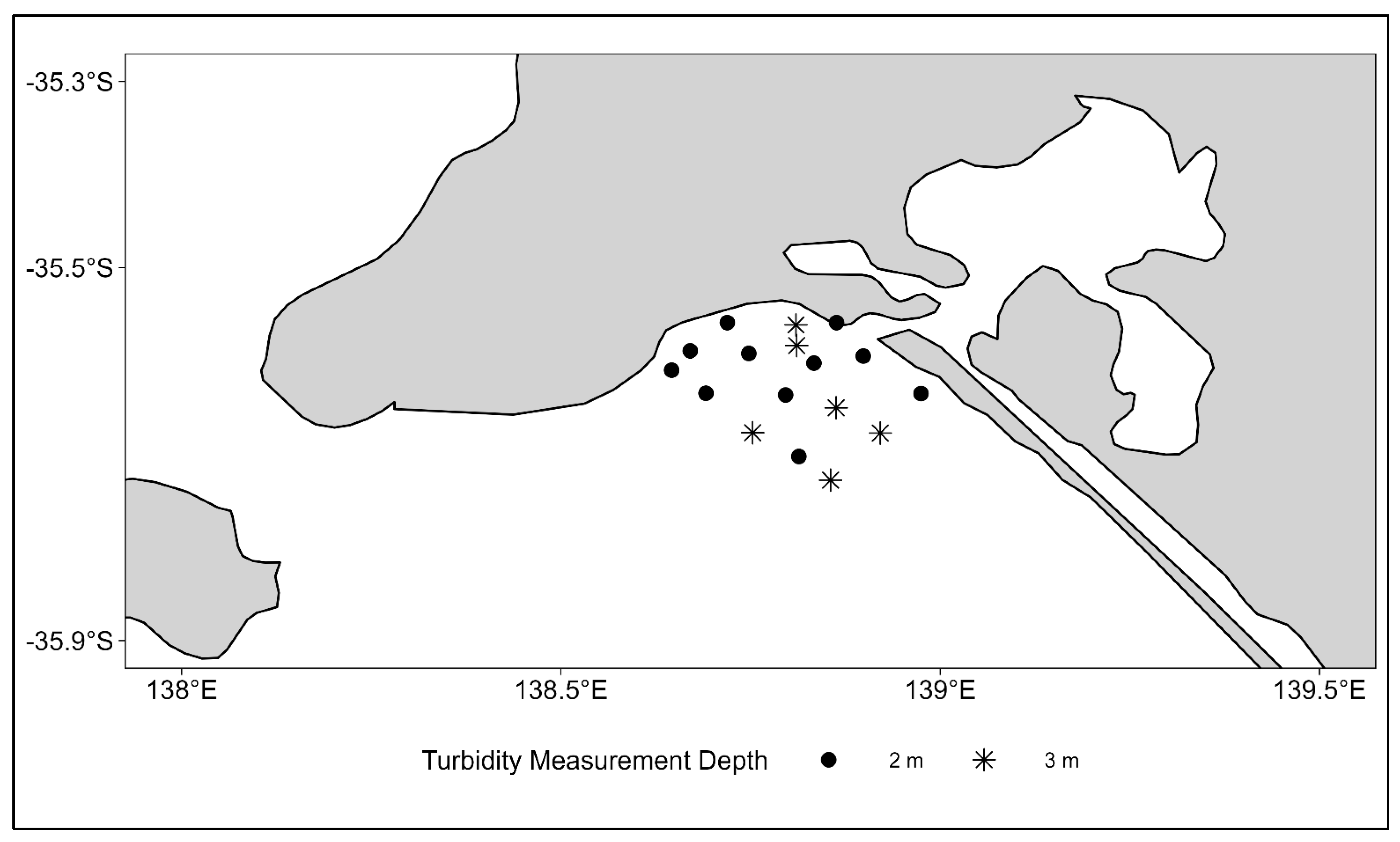
2.3.2. In Situ Turbidity Data

In situ turbidity was measured by a collaborative research team during two periods: during high riverine discharge (21–23 February 2022) and post-flood (31 May–1 June 2022). The team, focused on the flood water’s coastal impacts, included members from the South Australian Research and Development Institute (SARDI), the Commonwealth Scientific and Industrial Research Organisation (CSIRO), and the University of Adelaide. The data were measured using conductivity, temperature, and depth (CTD) casts, specifically with a Seabird SBE 19plus profiler (Seabird Scientific, Seattle, DC, USA). This profiler, fitted with an SBE EcoFLNTU sensor, measured instantaneous turbidity values at 1 m depth increments. The data were quality assured and quality controlled to Australia’s Integrated Marine Observing System (IMOS) standards. These in situ turbidity data were provided for use in this study to assess the correlation between in situ and Kd490 estimates. The turbidity data were measured in NTUs, with the values based on factory calibration.

Due to the surface-level nature of Kd490 estimates, in situ turbidity data were extracted to the surface-most measurement. This extraction provided each CTD cast location a singular turbidity value, alongside the depth of measurement. These depths of turbidity data were either 2 or 3 m below the water’s surface.

Additional information extracted from the QA/QC data was the profile ID, date, time, latitude, and longitude, providing spatial and temporal context to the data. This extracted data were formatted accordingly into two datasets representative of the two measurement periods, to be used for the correlation assessments to follow.

2.4. The Magnitude of the Sediment Plume and the Kd490 Anomaly

Total discharge data, calculated through the compilation of recorded discharge at all five of the barrages located within the Lower Lakes, were provided by the same collaborative research team for the assessment of how sediment plume dynamics were affected by discharge rates. The locations of these five barrages relative to the Murray Mouth and the Lower Lakes system are illustrated in Figure 6.

The data provided possess a total daily discharge rate in megalitres, which was converted into the equivalent flow rate in metres cubed per second. The accuracy of the discharge data was compromised on days with higher volumes, as water levels exceeded the height of the barrage walls, allowing discharge to flow over. Although this has been accounted for with calculated “seepage volumes” being added to the daily flow at each barrage by the data provider, it likely maintains a level of error. Despite this unknown level of accuracy, the provided data are crucial, being the only continuous dataset adjacent to the Murray Mouth. For this analysis, total discharge data were confined to a period representative of the flood, starting on the 1 August 2022 and ending on the 30 June 2023.

The calculation of the significant Kd490 area across the defined flood period was conducted using the processed raster dataset. A pixel was classified as exhibiting significant Kd490 levels when its value exceeded the pixel-specific 95th percentile of long-term (2002–2022) monthly Kd490 values. This operational definition enabled the identification of periods of anomalously high turbidity. The area of significant Kd490 was then calculated by summing the known surface area of all pixels exceeding this threshold within each 8-day composite period (see Equation (1)). This percentile-based approach accounts for spatial variability in baseline turbidity, allowing the detection of localised anomalies rather than relying on a uniform global threshold.

Significant Kd490 area = Σ (A_i), for all i where Kd490_i > kd_95

(1)

where A_i = area of pixel i; Kd490_i = Kd490 value of pixel i; and kd_95 = 95th percentile of the monthly Kd490 values for pixel i.

Restricting the application of Equation (1) to the spatial extent shown in Figure 7 enables the targeted detection of the River Murray sediment plume, while minimising the influence of unrelated water quality anomalies. This spatial constraint is appropriate given the lack of additional major freshwater inflows or turbidity-inducing features within the defined area.

The deviation of median Kd490 levels within the Murray Mouth zone (Figure 1 and Figure 7) from the monthly adjusted reference range was illustrated utilising the zonally processed dataset. The median Kd490 (kd_z50) for the Murray Mouth zone was plotted for each 8-day period. The visualisation of these data allows for the identification of the Kd490 levels across the flood event and their levels relative to a robust monthly adjusted reference range or “normal” levels of Kd490 for that month.

To assess the correlation between total discharge data and the two dependent variables of the significant Kd490 area and median Kd490 the datasets were plotted individually against total discharge rates. The two dependent variables were broken into two subsets of data and plotted accordingly: points preceding or following the day of peak discharge (29 January 2023). We utilised a linear model’s coefficients of determination (R²) to examine how much of the variation in the plume area could be explained by discharge. Pearson’s correlation coefficient for each relationship plotted was then performed to offer further insights into the correlation of the X and Y variables.

2.5. Temporal and Spatial Distributions of the Sediment Plume

2.5.1. Visualisations of Kd490 Estimates

To quantify and visualise the spatio-temporal dynamics of the flood-induced sediment plume both the Kd490 and significant Kd490 representing the sediment plume were plotted at “weekly” periods. The summarised raster dataset allowed for the visualisation of Kd490 and the subsequent plume through two key visualisation methods. These two methods are through plotting Kd490 pixel values and through discretely plotting pixels at which Kd490 is greater than the reference 95th percentile.

Each pixel of acceptable quality in coastal waters possesses a Kd490 value for every 8-day composition period. This allows for the plotting of Kd490 intensities across a region on a continuous scale. To enhance the visualisation of Kd490, the data are transformed into a logarithmic scale, log₁₀(Kd490), helping to highlight relative differences between pixels without compromising the dataset. Using the explained logarithmic transformation of log₁₀, Kd490 values for each 8-day period were plotted between 1 August 2022 and 30 June 2023. These plotted 8-day values of turbidity illustrate how Kd490 values varied spatially and in intensity across the 2022–2023 flood event.

To illustrate the Kd490 anomaly across the flood event and consequently understand the spatio-temporal dynamics of the sediment plume, the pixel-based dataset was utilised. The 95th percentile of the reference data (kd_95) was used in a comparison applied to each Kd490 pixel value for each 8-day period within the dataset. This comparison is presented in Equation (2), where the result indicates whether each pixel’s Kd490 value exceeds the 95th percentile of the reference data. Although not stored as a new variable, this comparison is visualised in the plot, denoted as “kd_gr_95pct”.

kd_gr_95pct = Kd490 > kd_95

(2)

The comparison of each Kd490 value against the 95th percentile of the reference data (kd_95) resulted in a discrete determination for each pixel—whether the Kd490 value exceeded the 95th percentile. This determination was visualised to quantify the spatial distribution of the Kd490 anomaly and, consequently, the sediment plume, on a “weekly” temporal scale. Although this visualisation utilises the same Kd490 estimates as the earlier log10(Kd490) visualisations, it provides deeper insights into the spatio-temporal dynamics of the plume by highlighting where and when Kd490 values exceeded the 95th percentile of the reference data.

2.5.2. The Horizontal Spreading of the Surface Sediment Plume

To assess the correlation of turbidity to distance from the Murray Mouth, the location of the Murray Mouth was defined as the point 138.88°, −35.56°. This definition allowed for the distance of each CTD cast location to the Murray Mouth to be calculated. The in situ turbidity dataset was selected for this assessment over Kd490 due to the point nature of the dataset compared to the pixel nature of the Kd490 estimates, providing uncertainty in the computation of distance from the Murray Mouth, as well as being the dataset of recognised accuracy. We fit linear models to subsets of the two sample depths of turbidity to assess the correlation of turbidity to distance from the Murray Mouth and whether that varies with the depth of turbidity data. This process was performed individually for both periods of in situ measurement and assessed how proximity to the discharge source affects sediment plume intensity in the coastal zone. Analysis of these values will detail the strength and nature of the correlation between turbidity and distance from the Murray Mouth based on the provided in situ dataset.

2.6. Correlation of Kd490 to In Situ Turbidity Data

To support the use of Kd490 estimates as an indicator for sediment plume identification the correlation of Kd490 to in situ turbidity data was assessed. This assessment identifies whether Kd490 is a robust product, as turbidity is understood to be strongly correlated with sediment plume presence, as introduced. The following analyses were performed using the processed pixel-based Kd490 and in situ turbidity datasets, processed from the downloaded MODIS Aqua Kd490 estimates and the provided in situ CTD cast data, as explained in Section 2.3.

Initially, to understand the spatial distribution of the data within Long Bay the CTD cast positions were plotted for both measurement periods, using their inherent latitude and longitude coordinates (Figure 8 and Figure 9). The variation in depth of each in situ turbidity measurement was represented through variation in the shape of the CTD cast location points, allowing for visual identification of any spatial trends in the depth of data provided.

Figure 8 and Figure 9 display the spatial distribution of the in situ turbidity data measured during two periods: high riverine discharge and post-flood event. These figures illustrate the reduction from 30 to 17 CTD cast locations from high discharge to post-flood event measurement periods. The depth at which the surface-most turbidity values (2 m or 3 m) were measured shows no consistent pattern, with many corresponding points exhibiting changes in depth across measurement periods. After examining the spatial distribution of in situ turbidity data, the focus shifted to evaluating the correlation of paired Kd490 and in situ turbidity data, shedding light on the relationship between these variables and their implications for understanding water quality dynamics.

To assess the correlation of the two datasets, a subset of Kd490 estimates was first extracted to match the locations of in situ measurements. This extraction selected Kd490 values of pixels that aligned with CTD cast locations from the corresponding 8-day period. Notably, the 8-day period corresponding with the post-flood in situ measurements contained gaps in the Kd490 estimates due to the masking of poor-quality pixels. These gaps coincide with two in situ turbidity points, reducing the number of spatially paired data points for the post-flood assessment from 17 to 15 pairs.

The extracted Kd490 values were then added to the processed in situ dataset as a new variable. Next, the Kd490 estimates and the in situ turbidity data were plotted against each other, grouped by the depth of the turbidity measurements. This depth-based grouping (2 m and 3 m) allowed for an individual assessment of the relationship between Kd490 and in situ turbidity at different depths.

Linear models were fitted to both depth subsets to evaluate the correlation of Kd490 and in situ turbidity data at the two measured depths. This analysis was performed separately for both periods of in situ measurement periods: during high riverine discharge and post-flood event.

We defined the mouth of the Murray as the point 138.88°, −35.56° to assess the correlation of turbidity with distance from the mouth. This definition allowed for the distance of each CTD cast location to the Murray Mouth to be calculated. The in situ turbidity dataset was selected for this assessment over Kd490 due to the point nature of the dataset compared to the pixel nature of the Kd490 estimates, providing uncertainty in the computation of distance from the Murray Mouth, as well as being the dataset of recognised accuracy. We fit linear models to subsets of the two sample depths of turbidity to assess the correlation of turbidity to distance from the Murray Mouth and whether that varies with the depth of turbidity data. This process was performed individually for both periods of in situ measurement and assessed how proximity to the discharge source affects sediment plume intensity in the coastal zone.

3. Results

3.1. The Magnitude of the Sediment Plume and the Kd490 Anomaly

To understand the magnitude of the flood-induced sediment plume, a time series of the Murray’s discharge data was produced alongside the time series of the significant Kd490 area (km²) and the deviation of Kd490 at the Murray Mouth from a monthly adjusted reference range. These time series presented in Figure 10a–c illustrate the temporal variations in flood impacts on the two dependent variables, suggesting differing levels of correlation and varying durations of influence.

Figure 10a illustrates the high variability in river discharge, particularly leading up to the flood, with periods of low to no flow through the barrages. These periods are likely due to reduced river flows combined with the operation of the barrage network restricting flow.

Figure 10b,c both display visible spikes in the respective significant Kd490 area and the median Kd490 at the Murray Mouth, which align temporally with a notable increase in the river discharge shown in Figure 10a. The significant Kd490 area reached a maximum extent of 13,681 km² for the 8-day period beginning on 11 December 2022, whilst the median Kd490 at the Murray Mouth reached a maximum value of 1.22 m⁻¹ for the 8-day period beginning on 9 January 2023. The maximum monthly varying reference Kd490 at the Murray Mouth was 0.41 m⁻¹ for March, set at the 95th percentile of all March observations for the preceding ~20 years of MODIS Kd490 estimates.

Although Figure 10a–c indicate a likely correlation between the riverine discharge rates and the two variables of the significant Kd490 area and the median Kd490 at the Murray Mouth, Figure 11 and Figure 12 statistically assess these potential correlations.

Figure 11 assesses the correlation of the significant Kd490 area to the total discharge rates and shows that just above 50% of the variance in the significant Kd490 area is explained by the discharge rate for both periods before (R² = 0.52) and after (R² = 0.53) the date of peak discharge. When all dates are combined, the explained variance drops to 28% (R² = 0.28), highlighting the variability in the plume area response across varying stages of the flood event.

Figure 12 assesses the correlation of the median Kd490 at the Murray Mouth to the total discharge rates. Here, 48% (R² = 0.48) and 75% (R² = 0.75) of the variance in the median Kd490 is explained by the discharge rates for the periods before and after the date of peak discharge, respectively. When the two periods are combined, discharge explains 50% (R² = 0.50) of the variance in the median Kd490, again highlighting a varied relationship at varying stages of the flood event.

3.2. The Temporal and Spatial Distributions of the Sediment Plume

3.2.1. Visualisations of Kd490 Estimates

To understand the temporal and spatial distribution of the flood-induced sediment plume, visualisations of the Kd490 estimates were produced as Kd490 pixel values and significant Kd490 pixels (sediment plume). These visualisations are illustrated in Figure 13 and Figure 14.

Figure 13 and Figure 14 illustrate the temporal variability of the sediment plume, centred on the period of the peak Kd490 distribution from November 2022 to February 2023. The variation between the visualisations of Kd490 estimates and significant Kd490 estimates is clearly shown between Figure 13 and Figure 14, with visible increases in Kd490 values throughout Figure 13 at offshore and southwestern locations which were not computed as significant (true) in Figure 14.

This is because many increases in Kd490 occur within seasonal expectations, which are accounted for by the reference data’s 95th percentile. For a Kd490 value to be deemed significant, it must exceed this reference 95th percentile, as seen throughout Figure 14. The abundance of significant Kd490 pixels in Figure 14 highlights the magnitude of the flood-induced sediment plume, visualising the same information plotted numerically in Figure 10b. Figure 13 illustrates the experienced k490 values, while Figure 14 shows the Kd490 anomaly.

Figure 14 shows that the plume’s distribution changes throughout the flood event, varying between westerly and easterly migrations and exhibiting variations in how far offshore the plume spread before dissipating below significant Kd490 levels. A consistent feature of the sediment plume at its most prominent distribution was its presence throughout the Backstairs Passage, from early December 2022 when the plume grew significantly to early February 2023 when the plume’s area decreased with lower discharge rates.

A likely reason for the plume’s persistence through the Backstairs Passage is that the passage is characterised by strong surface currents of up to 1.2 m/s, which generally operate just below 1 m/s flow velocities [67,68,69]. These flow velocities are part of a clockwise eddy formation that operates within the passage, likely subsequently “sucking” the surface plume through the passage and into the Gulf St Vincent.

Kd490 estimates showed two contradictions to the western movement of the sediment plume in early December 2022 and, more prominently, in early February 2023. In early February 2023, the plume is shown to migrate eastward, stretching alongshore as a continuous feature to as far east as the 42 Mile Crossing. This shift to a eastern migration is supported by the visible disconnect of plume areas in Long Bay and through the Backstairs Passage, illustrated in Figure 14, panel 18 February 2023.

Once the plume entered the base of Gulf St Vincent, it maintained a westward orientation, with Kd490 values decreasing but remaining significant. Fragments of a significant Kd490 (sediment plume) observed across several Figure 14 panels, especially those coupled with gaps in the data due to cloud cover, indicate potential noise in the data.

3.2.2. The Horizontal Spreading of the Surface Sediment Plume

The correlation of in situ turbidity values to the distance of each data point from the Murray Mouth was assessed for all in situ measurements across two periods in 2023 (Figure 15). One of the key differences in the in situ data measured across the two different measurement periods is inherently the distances from the Murray Mouth that CTD casts were positioned, with greater distances and point densities measured during the high discharge measurement period in February. The greatest distance between a CTD cast position and the Murray Mouth was 40.6 km during high riverine discharge and 21.8 km in the post-flood event.

The calculation of the coefficient of determination for the February high riverine discharge event indicates that distance from the Murray Mouth explains 43% (R² = 0.43) of the variance in turbidity data measured across both depths. When analysed separately, distance explains 73% (R² = 0.73) of the variance at the 2 m depth and 34% (R² = 0.34) at the 3 m depth, with both showing a negative correlation. The computed Pearson’s correlation coefficients support this trend, with the combined data producing a value of −0.66, the 2 m depth is −0.85 and the 3 m depth is −0.58.

In contrast, during the May–June post-flood event, the coefficient of determination indicates that the distance from the mouth explains only 2% (R² = 0.02) of the variance in turbidity across both depths. When considered separately, distance explains 2% (R² = 0.02) of the variance at the 2 m depth and 94% (R² = 0.94) at the 3 m depth. Corresponding Pearson’s correlation coefficients are −0.03 for the combined data (indicating no linear relationship), 0.41 for the 2 m depth (moderate positive correlation), and −0.96 for the 3 m depth (very strong negative correlation).

3.3. Correlation of Kd490 to In Situ Turbidity Data

To better understand if the Kd490 results are reasonable and accurate in South Australian waters, the Kd490 estimates were compared with the in situ turbidity data measured across two periods. Note, that as stated in Section 2.3.2, the in situ data are derived from instantaneous measurements at depth intervals of 1 m and are representative of a precise X and Y position. In contrast, the Kd490 estimates provide an 8-day composite value, representative of a coarse 4616 m resolution pixel. Unlike the in situ data, Kd490 only serves as an estimate of the rate that light at 490 nm is attenuated with the depth from the surface.

Figure 16 illustrates the correlation between the Kd490 estimates and in situ turbidity data during the two measurement periods: during high riverine discharge and the post-flood event. During the high riverine discharge period, the coefficient of determination (R²) indicates that Kd490 estimates explain 51% of the variance in turbidity across both measured depths (R² = 0.51). Specifically, Figure 16 shows that Kd490 explains 85% of the variance in turbidity at the 2 m depth (R² = 0.85) and 28% at the 3 m depth (R² = 0.28), with both correlations being positive and linear. To complement these insights, Pearson’s correlation coefficients were calculated to assess the strength and direction of these linear relationships. A moderately strong positive correlation (r = 0.71) was computed for the combined depth data during the high riverine discharge. For the individual depths post-flood, the correlation at 2 m was strong (r = 0.92) and was moderate at the 3 m depth (r = 0.53).

During the post-flood period, the coefficient of determination (R²) indicates that Kd490 estimates explain 23% of the variance in the turbidity data measured across both depths combined (R² = 0.23). Specifically, Figure 16 shows that Kd490 explains only 5% of the variance at the 2 m depth (R² = 0.05) while explaining a much higher 89% at the 3 m depth (R² = 0.89). The Pearson’s correlation coefficient for the combined depth data was r = 0.48, indicating a moderate positive correlation with the post-flood event. However, when analysed separately, the correlation at the 2 m depth was weak and negative (r = −0.21), while at 3 m it was strong and positive (r = 0.94).

4. Discussion

4.1. The Magnitude of the Sediment Plume and the Kd490 Anomaly

The increase in both the significant Kd490 area and the median Kd490 at the Murray Mouth appears to correspond with the rise in riverine discharge during the 2022–2023 flood event, indicating a likely positive correlation between the riverine discharge, sediment plume area, and water quality. Interestingly, the maximum sediment plume spatial extent (13,681 km²) and the Kd490 value at the Murray Mouth (1.22 m⁻¹) did not coincide within the same or consecutive 8-day periods. The maximum sediment plume extent was observed during the 8-day period beginning on 11 December 2022, while the maximum Kd490 value occurred in the period beginning on 9 January 2023. This temporal disparity may reflect flood-induced sediment plume dynamics, where the sediment load and type change throughout a major discharge event. The head of the flood will generally carry the greater and coarser sediment load due to increased flow speeds and volumes through the associated river system [70]. In contrast, the sediment plume area responds more gradually, as it is a product of both time and sediment supply.

Additionally, the temporal disparity between the sediment plume maximum extent and the maximum Kd490 is influenced by the two variables, representing data from different spatial areas with distinct relationships to riverine discharge. The significant Kd490 area is computed from the greater Long Bay ROI (Figure 7), while the median Kd490 is derived from the Murray Mouth zone specifically (Figure 1).

The 2022–2023 flood-induced Kd490 anomaly’s magnitude and persistence in sediment plume formation are evident in Figure 10c. The time series shows that the median Kd490 at the Murray Mouth exceeded the monthly varying reference level for twelve consecutive periods, from the period beginning on 19 December 2022 to the period beginning on 22 March 2023. During this period, Kd490 levels were at times more than three times the corresponding monthly reference level. Notably, this period of significance is not due to a reduction in the number of pixels used in calculating the median Kd490 (N_obs). Figure 10c confirms this by colour-coding each point based on its N_obs value, which consistently shows four or five observations out of five for all 8-day periods except one, which has three. These values are comparable to those seen before and after the period of Kd490 significance.

The statistical analysis of the relationship between the significant Kd490 area and riverine discharge, as shown in Figure 11, reveals a positive linear relationship. The R² value increases when focusing on periods before and after the peak discharge, with the variance explained by the riverine discharge rising from 28% to 52% and 53%. This suggests that the relationship between discharge rates and the sediment plume area varies at different stages of the flood event. These findings align with previous studies, which highlight the relationship between discharge rates and the sediment plume area and the variance explained in these relationships [17,22,48,71].

Similarly, the relationship between the median Kd490 at the Murray Mouth and riverine discharge, illustrated in Figure 12, shows a positive linear relationship. The R² value for the entire dataset is 0.50, indicating that 50% of the variance in the median Kd490 is explained by riverine discharge. When focusing on the data before the peak discharge, the variance explained increases to 48%, while the variance explained after the peak discharge rises to 76%. This suggests that the relationship between the discharge and Kd490 becomes more pronounced in the latter stages of the flood, as the flow and sediment load stabilise. These findings are consistent with the literature indicating that water quality is closely linked to riverine discharge and the sediment it transports [5,9,18,21,48].

These findings provide statistical evidence supporting Petus et al. (2014), who state that riverine discharge controls the sediment plume spatial extent and water quality [15]. High discharge events typically produce highly turbid inner plumes, with higher Kd490 values near the Murray Mouth, possibly reflecting the expanding jet core of river flow [72]. Further offshore, winds and currents likely become the dominant drivers of plume dynamics as it disperses into the complex coastal environment.

Limitations to these conclusions include the temporal resolution of Kd490 estimates, which provides a single significant Kd490 area and median Kd490 estimate for each 8-day composite period. Spatial resolution also impacts the results, particularly the median Kd490 values as these depend on both the number and values of pixels included in the median computation (up to a maximum of five pixels). This number is a function of the delineated zone’s area representing the Murray Mouth and is influenced by the data availability, such as cloud cover.

4.2. The Temporal and Spatial Distributions of the Sediment Plume

4.2.1. Visualisations of Kd490 Estimates

The observed differences between Figure 13 and Figure 14 result from the use of monthly reference values in determining the Kd490 significance. Figure 14’s focus on significant Kd490 anomalies, rather than absolute values, underscores the magnitude of the flood-induced sediment plume. It is crucial to note that Figure 13 captures the actual Kd490 values experienced during the event, while Figure 14 isolates deviations from expected patterns.

Figure 17 illustrates three periods when the plume was in a typical (B1 and B2) or distinct (C) position. In the first case (B1) the plume is driven entirely by riverine discharge during the rising peak of the flood, exhibiting an arcuate lobe commonly associated with river mouth jets. In the second case (B2), the plume is driven west and enters the Backstairs Passage. In the third case (C), which is far less common, north-westerly winds had been blowing for some days and drove the plume along the coast to the southeast. Figure 17C illustrates the temporal evolution of this plume behaviour, from its typical position to a south-eastward migration.

The persistent presence of the sediment plume in Backstairs Passage, from December 2022 to February 2023, likely results from the strong surface currents characteristic of this area. These currents reach up to 1.2 m/s flow velocities, whilst generally operating just below 1 m/s, and form part of a clockwise eddy system [67,68,69]. Once sufficient westward migration of the plume has occurred, bringing the sediment plume within the eddy’s area of influence, these currents could be drawing the surface plume through the passage and into Gulf St Vincent.

This hypothesised dynamic contrasts with the two eastward migrations of the sediment plume observed, with the most significant event in early February 2023. If during this easterly migration event the plume did not disconnect, then an argument for multidirectional plume dynamics could be made; however, this was not the case. This eastward shift forcing the plumes to disconnect was likely driven by significant surface winds emanating from the NE coupled with a change to discharge rates, as per Section 1.2 Future modelling or in situ measurements of the current flow in the passage and surface winds in the region could validate this derived hypothesis.

Interestingly, despite the eastward migration within Long Bay, the plume consistently maintained a westward orientation within Gulf St Vincent. This difference in the plume behaviour between the two regions may be attributed to persistent local currents and localised surface winds. The significant Kd490 values existing within Gulf St Vincent are much lower values then within Long Bay, as illustrated in Figure 13, although both regions maintain significance due to varying reference levels, with Long Bay possessing consistently greater values.

All observations regarding the sediment plume’s distribution are based on the inherently coarse spatial and temporal resolutions of the Kd490 estimates, whilst assuming the product’s accuracy in representing the sediment plume presence. The resolution limits fine-scale analyses, making it difficult to capture smaller-scale plume dynamics. These limitations are primarily due to the availability of higher-resolution satellite data and the resources required to process such data. With an increased access to higher-resolution spatial and temporal data, stronger and more detailed observations could be made. To enhance the sediment plume detection and assessment, higher-resolution satellite data, as well as ground truthing with in situ measurements, would be essential.

4.2.2. The Horizontal Spreading of the Surface Sediment Plume

The findings highlight a clear distinction between the correlation of the in situ turbidity data with the distance from the Murray Mouth during high riverine discharge and post-flood conditions. During high discharge, turbidity showed a consistent negative linear correlation with the distance from the mouth, as seen in Figure 15. This trend aligns with previous research by Aurin et al. (2013) and Kostaschuk et al. (1993), demonstrating that turbidity levels decrease as the sediment plume spreads from the point of discharge [4,73].

In contrast, post-flood data (also shown in Figure 15) revealed a weaker correlation at the 2 m depth, where distance only explained 2% of the variance in turbidity. This reduction in correlation is likely influenced by the very limited number of data points, narrower ranges of turbidity, and shorter offshore distances sampled during the post-flood period. The reduction in the turbidity data’s variability, as shown in

Table 1. Turbidity and Kd490 ranges for each in situ measurement period and depth. In situ data points from the post-flood measurement period that do not spatially correspond to a Kd490 cell value (2) are not included.

Data Subset	In Situ Turbidity Range (NTU)	Kd490 Range (m−1)
During high riverine discharge	0.47–9.04	0.18–0.91
During high riverine discharge 2 m	1.46–9.04	0.42–0.91
During high riverine discharge 3 m	0.47–8.70	0.18–0.91
Post-flood event	1.28–3.55	0.13–0.23
Post-flood event 2 m	1.63–3.55	0.15–0.18
Post-flood event 3 m	1.28–2.96	0.13–0.23

, is indicative of lower discharge rates and the absence of a significant sediment plume. Figure 8 and Figure 9 further illustrate this by showing a reduction in the sampling distance from 40.6 km offshore during the high discharge period to 21.8 km post-flood. Although a very strong correlation was found at the 3 m depth for the post-flood period, this was notably derived from only six data points.

The difference between the two measurement periods at the 2 m depth suggests that, while turbidity strongly correlates with distance during high discharge events, the relationship weakens once the plume dissipates and the range of Kd490 reduces. The post-flood period’s limited spatial and turbidity ranges likely reduce the reliability of the observed correlation. However, Figure 15 still supports the general trend that sediment plumes at the Murray Mouth decrease in concentration as they move further offshore.

In summary, the strong negative correlation observed during high discharge reflects the expected behaviour of sediment plumes dispersing from their source. Meanwhile, the weak or inconsistent correlation at the 2 m depth post-flood highlights the limitations of the reduced sampling coverage and the absence of a significant sediment plume.

4.3. Correlation of Kd490 to In Situ Turbidity Data

The results show notable differences in the correlation between the Kd490 and in situ turbidity data across the two periods of the high riverine discharge and post-flood event. During the high riverine discharge, the strong positive correlation at the 2 m depth, reflected by both R² and Pearson’s correlation coefficients, suggests that Kd490 is a reliable proxy for surface turbidity. This is consistent with Kd490’s role in measuring light attenuation in the water column, as light attenuates more quickly in turbid waters, with stronger attenuation occurring nearer the surface. However, at the 3 m depth, the correlation weakens, likely reflecting the limitations of Kd490 in capturing sub-surface variability when turbidity levels are elevated near the surface.

In contrast, the post-flood event is where the strongest correlation is observed at the 3 m depth and where Kd490 explains a larger percentage of the variance in turbidity (R² = 0.89), and Pearson’s correlation coefficient is 0.94. This reversal may be attributed to several hydrodynamic and optical factors. One possibility is the presence of residual turbidity at depth following the main flood event, as sediment-laden water settles or becomes entrained below the surface layer [74]. Another potential explanation is vertical stratification, where the water column becomes more layered after the peak discharge subsides, trapping turbid water at depth and decoupling surface conditions from sub-surface turbidity [75,76]. The reduced range of turbidity data during the post-flood measurement period (Table 1 and Figure 16) and the absence of a significant sediment plume may further weaken the correlation at 2 m, as the variability is too low for a strong statistical relationship to emerge.

The difference between depths and periods also points to the role of vertical mixing dynamics. During high discharge, an increased freshwater inflow and wave activity can enhance vertical mixing, leading to a more uniform distribution of turbidity in the upper water column and stronger surface correlation with Kd490 [16,77,78]. In contrast, calmer post-flood conditions may reduce mixing and allow fine sediments to settle, altering the vertical turbidity profile and shifting the strongest correlation deeper.

The variability between the two depths and measurement periods highlights several important factors. First, Kd490 does not directly measure turbidity but instead estimates the rate at which light attenuates in water at a wavelength of 490 nm. Therefore, differences in the water quality, plume presence, and sediment load are likely to influence Kd490’s effectiveness in estimating turbidity across different periods and depths. The strong correlations observed between Kd490 and turbidity, despite these complexities, provide valuable insights, but the differences in the spatial and temporal resolution between the point-based field measurements and the comparatively far coarser remote sensing Kd490 estimates also highlight the limitations.

The results underscore the need for more extensive field data to improve the understanding of Kd490’s correlation with in situ turbidity. The current analysis is based on only two measurement periods, each representing distinct stages of a flood event. Future studies should include more periods that capture different flood stages, increased spatial sampling, and consistent data point volumes to provide a more comprehensive understanding of the relationship between Kd490 and turbidity in South Australian waters. Despite these limitations, the strong correlations observed across the measurement periods demonstrate great potential for Kd490 to estimate surface turbidity. Given the dataset’s limitations, these findings still demonstrate its efficiency for monitoring nearshore turbidity dynamics.

4.4. Informing Management Strategies

The elevated turbidity and associated sedimentation resulting from the plume may degrade critical fish habitats, potentially causing immediate declines in local fish populations and leading to longer-term ecological effects. The evidence of immediate population impacts was prominent across the 2022–23 flood event, as stated in Section 2.1, with widespread marine mortality being a concern for both commercial and recreational fisheries. Furthermore, a reduced water clarity may deter tourism-related activities, with cases such as the 2022–2023 event seeing popular recreational beaches deemed unsafe.

By quantifying the spatio-temporal dynamics of sediment plumes, this study can support targeted monitoring during peak turbidity periods, inform the time-sensitive management of river discharge (e.g., barrage operations), and assist coastal managers in mitigating ecological and socio-economic impacts in vulnerable areas.

5. Conclusions

In conclusion, this study identifies the dynamics of the River Murray sediment plume during the significant flood event of 2022–2023. Through a combination of remote-sensing applications and in situ measurements, valuable insights have been gained into the temporal and spatial dynamics of the plume and the utilisation of the Kd490 product to accurately detect surface sediment plumes in South Australian waters. The key findings and their implications for future research and environmental management are as follows:

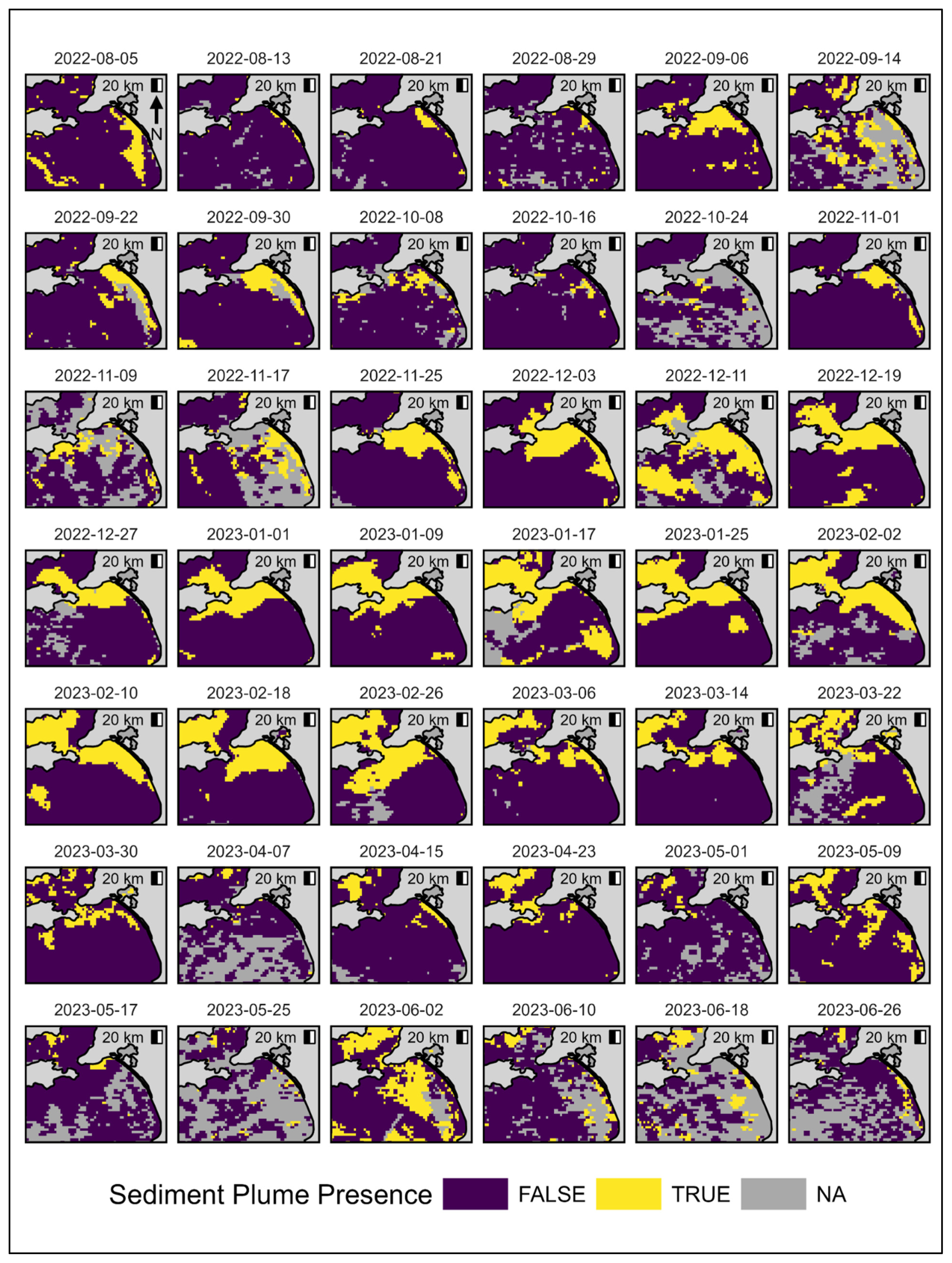
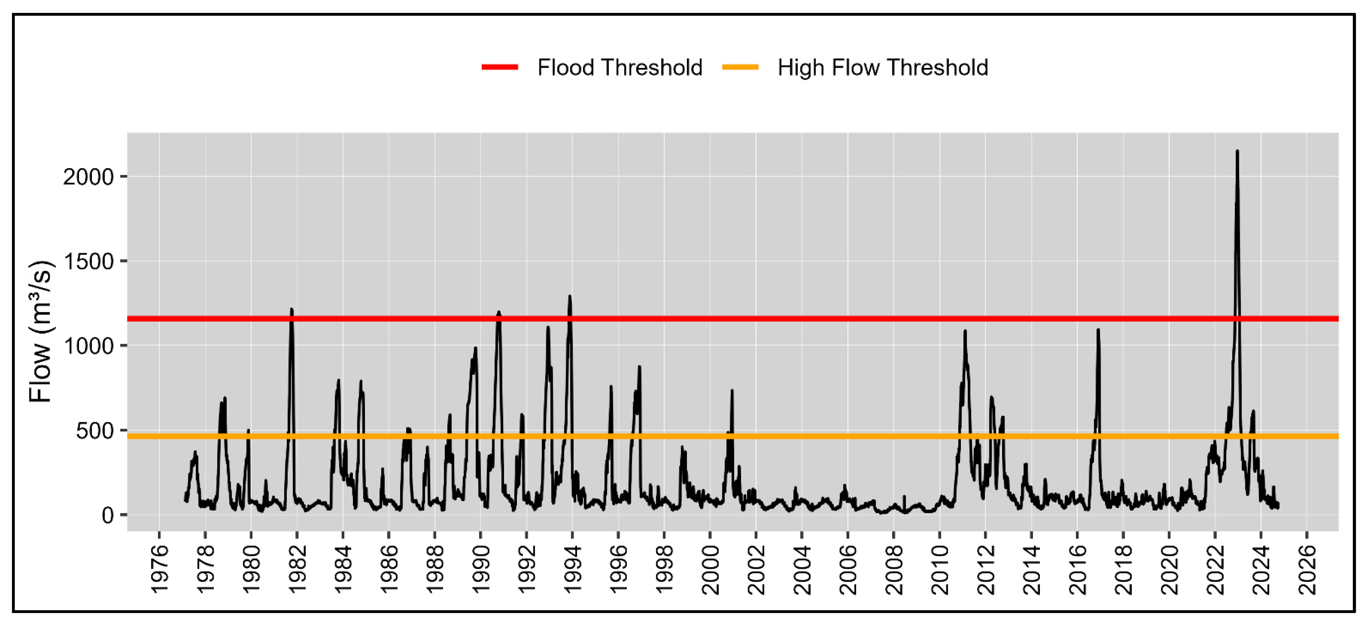
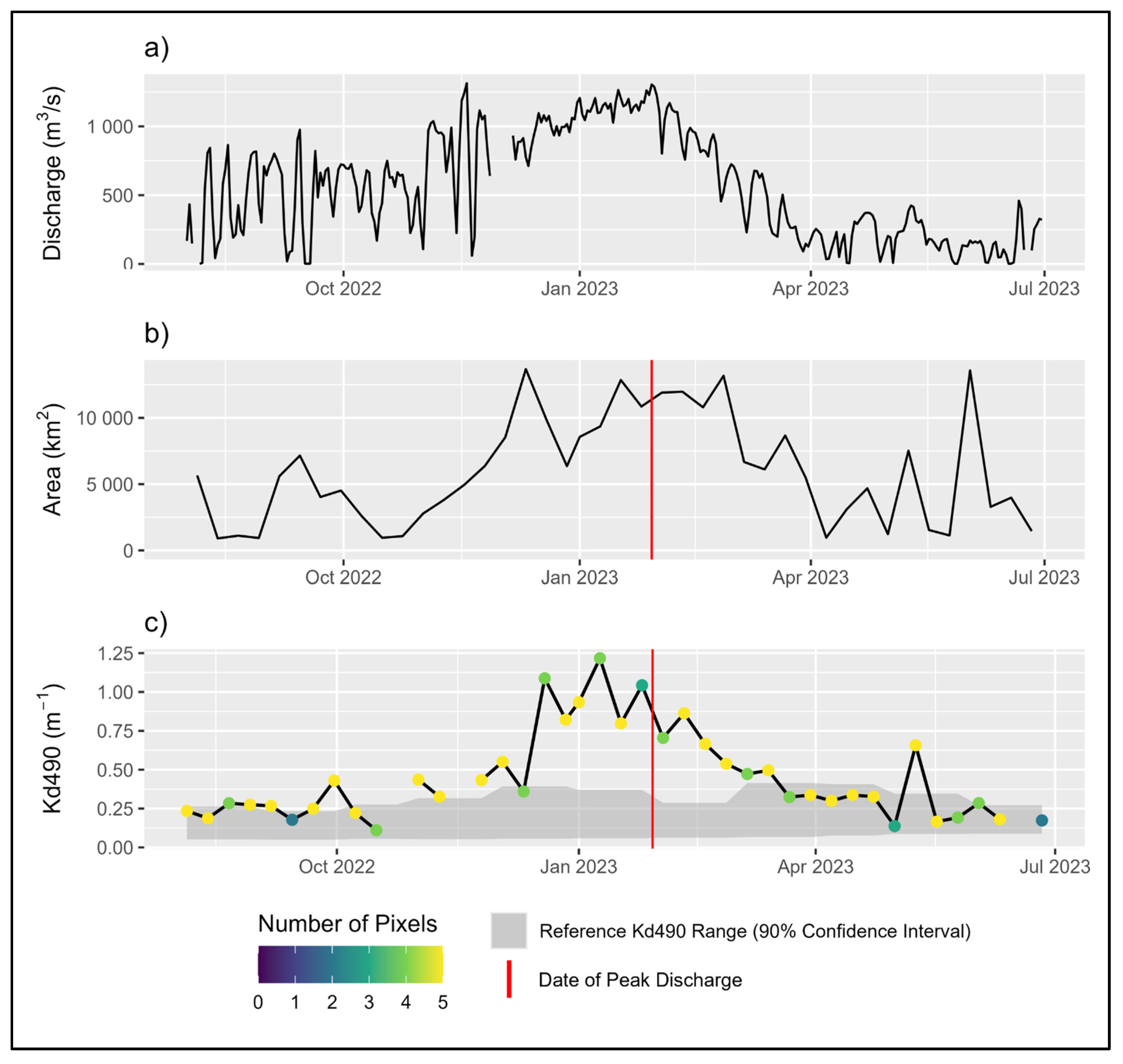
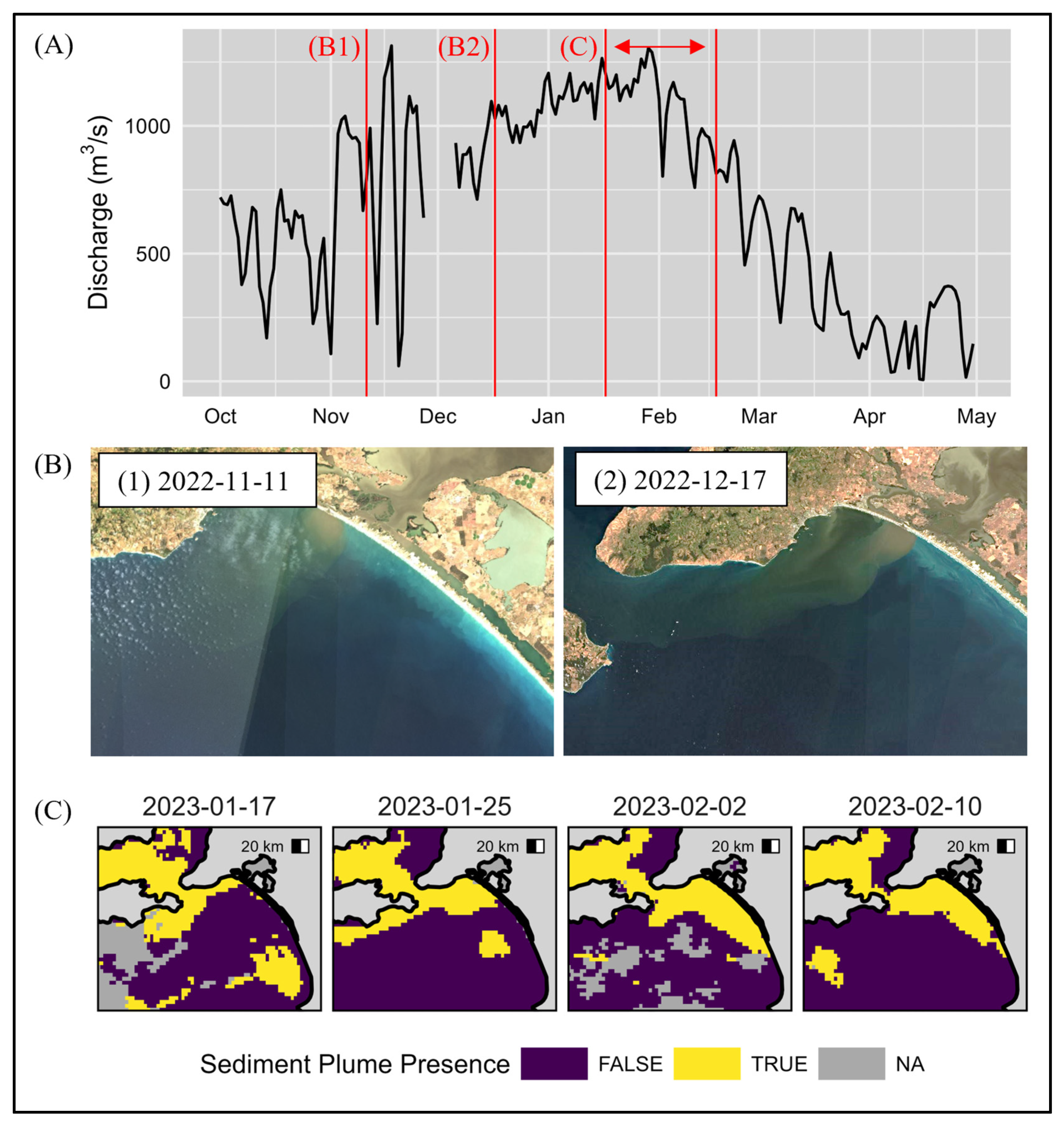
• The River Murray flood event of 2022–2023 led to a significant increase in riverine discharge from November 2022 to February 2023, peaking on 29 January with a daily flow rate of 1305 m³/s. Interestingly, the historically significant sediment plume within the coastal region reached its maximum spatial extent of 13,681 km² during the 8-day period beginning on the 11 December 2022, over a month before the peak discharge occurred.
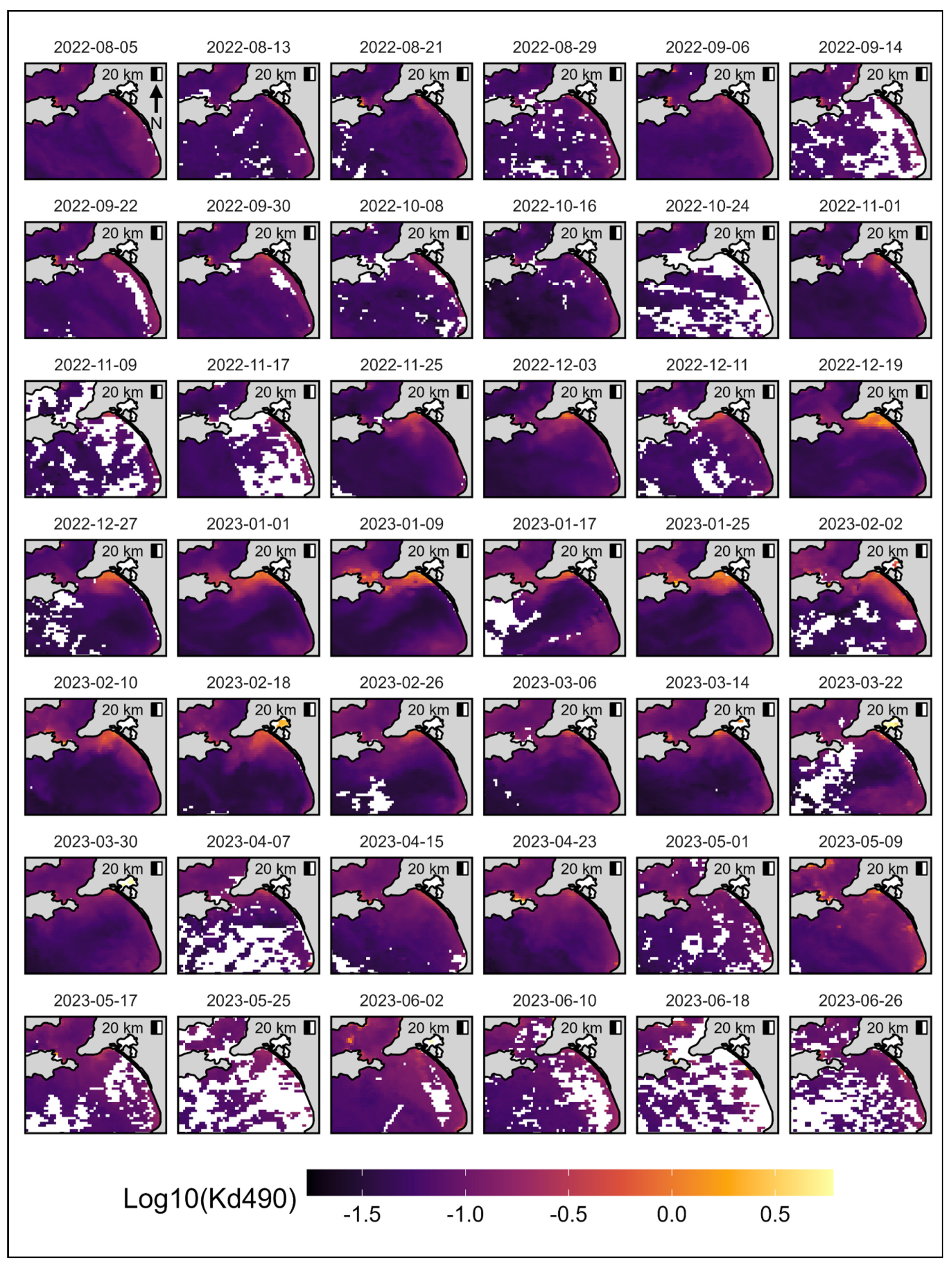
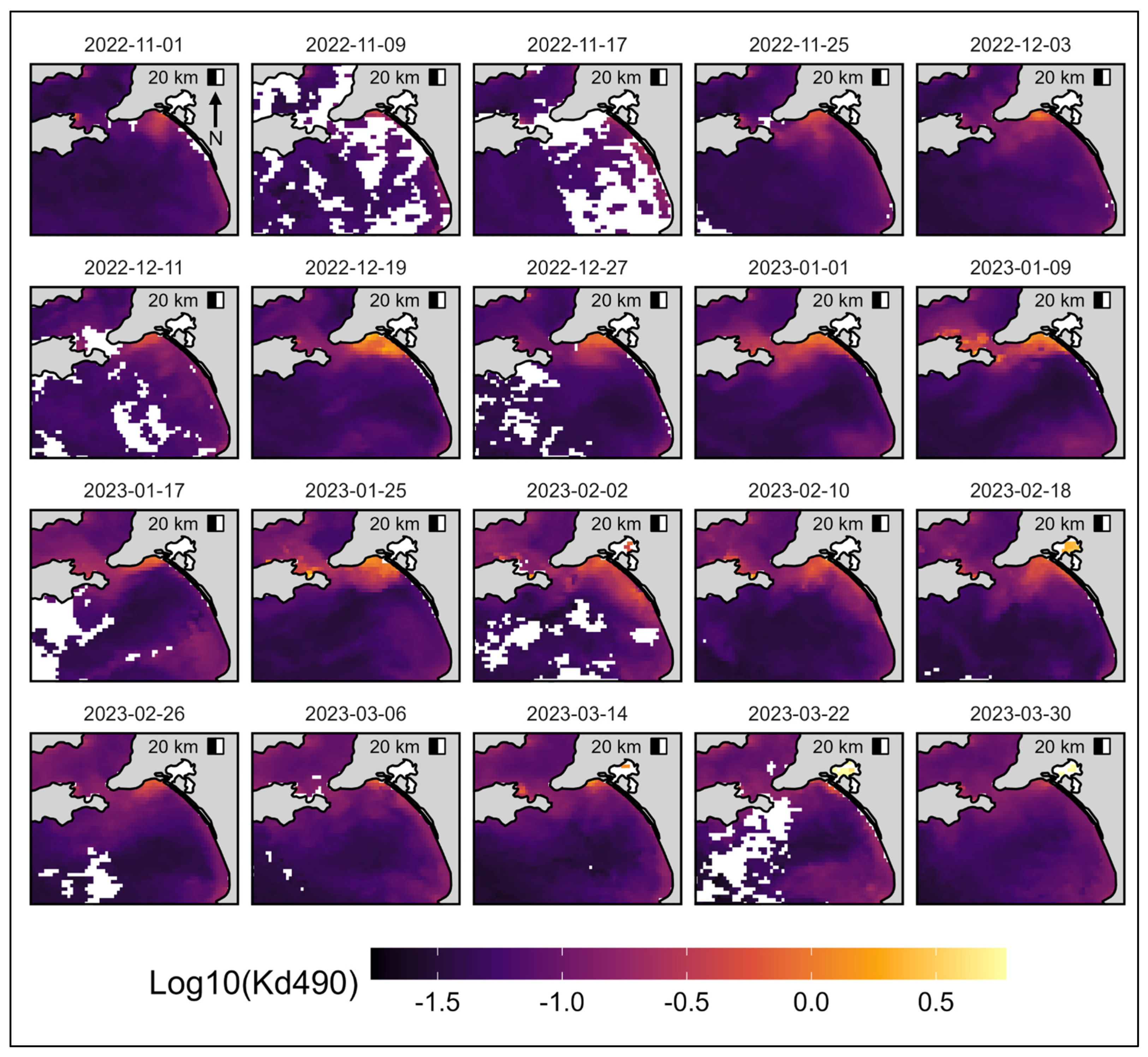
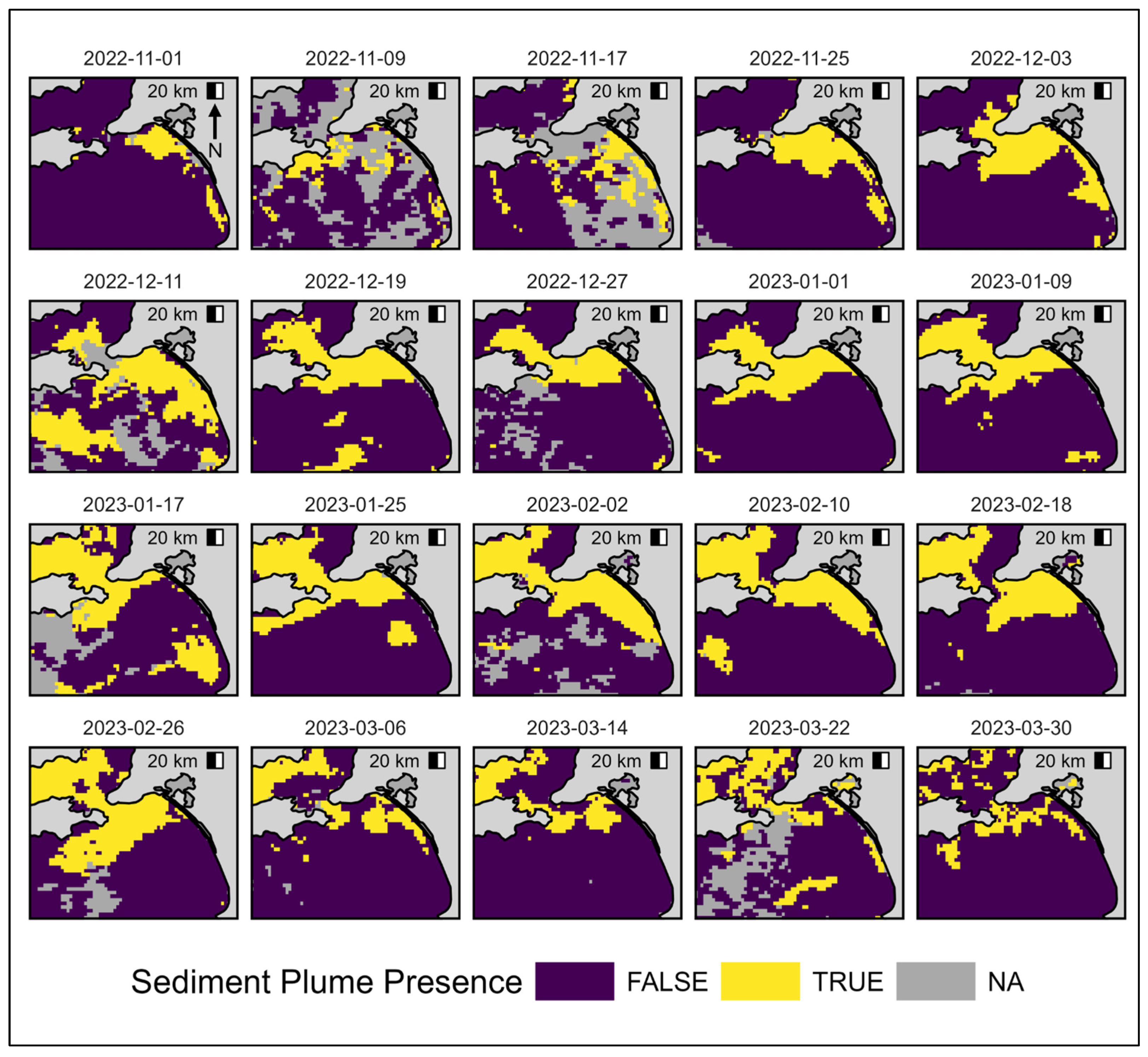
• Utilising the diffuse attenuation coefficient at 490 nm (Kd490) product alongside MODIS Aqua Ocean Color Level 3 satellite imagery, the temporal and spatial dynamics of the surface sediment plume were successfully mapped. The imagery shows a typical pooling of the plume in the northern corner of Long Bay and Encounter Bay and the westward persistence of the plume through Backstairs Passage into Gulf St Vincent, with periods of brief eastward migration.
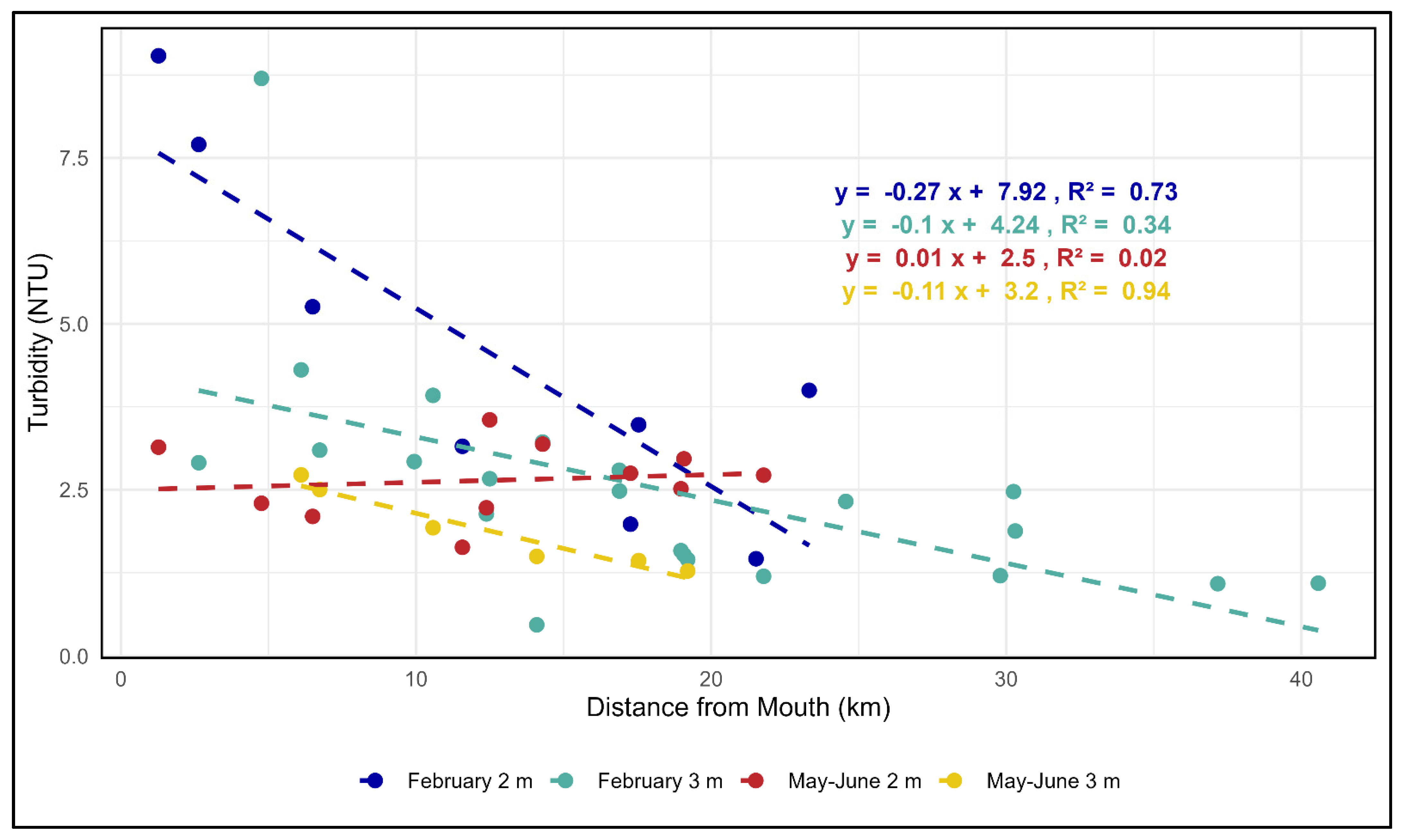
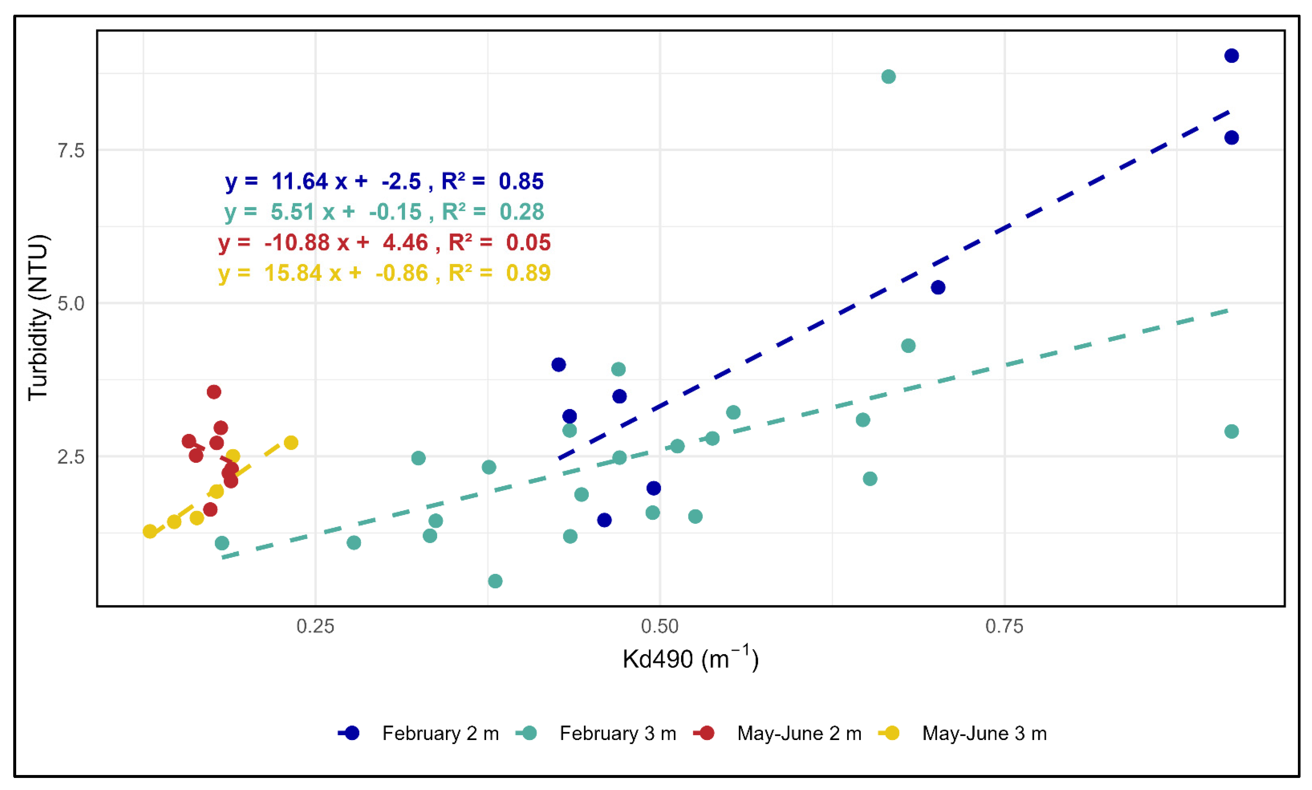
• The assessment of the relationship between Kd490 8-day data composites and two instantaneous in situ sampling periods of turbidity found strong positive linear correlations. Given the temporal and spatial mismatch of the two datasets along with the novelty of the product’s application within South Australian waters, this correlation is exceptional.
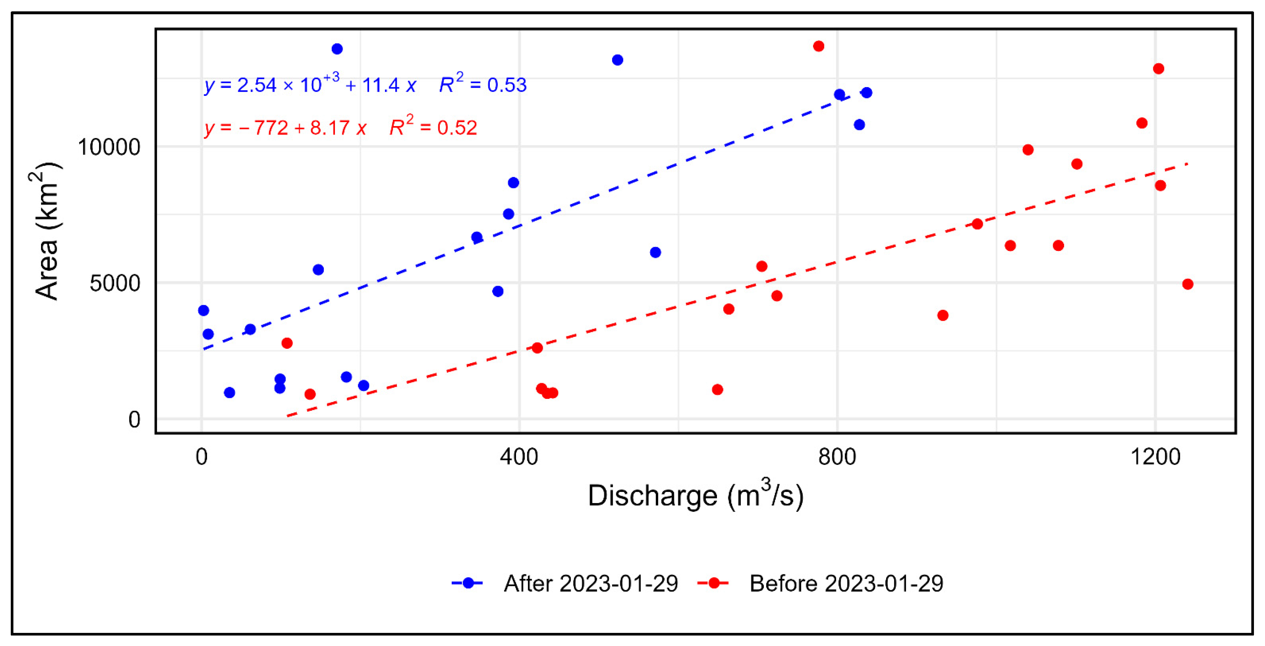
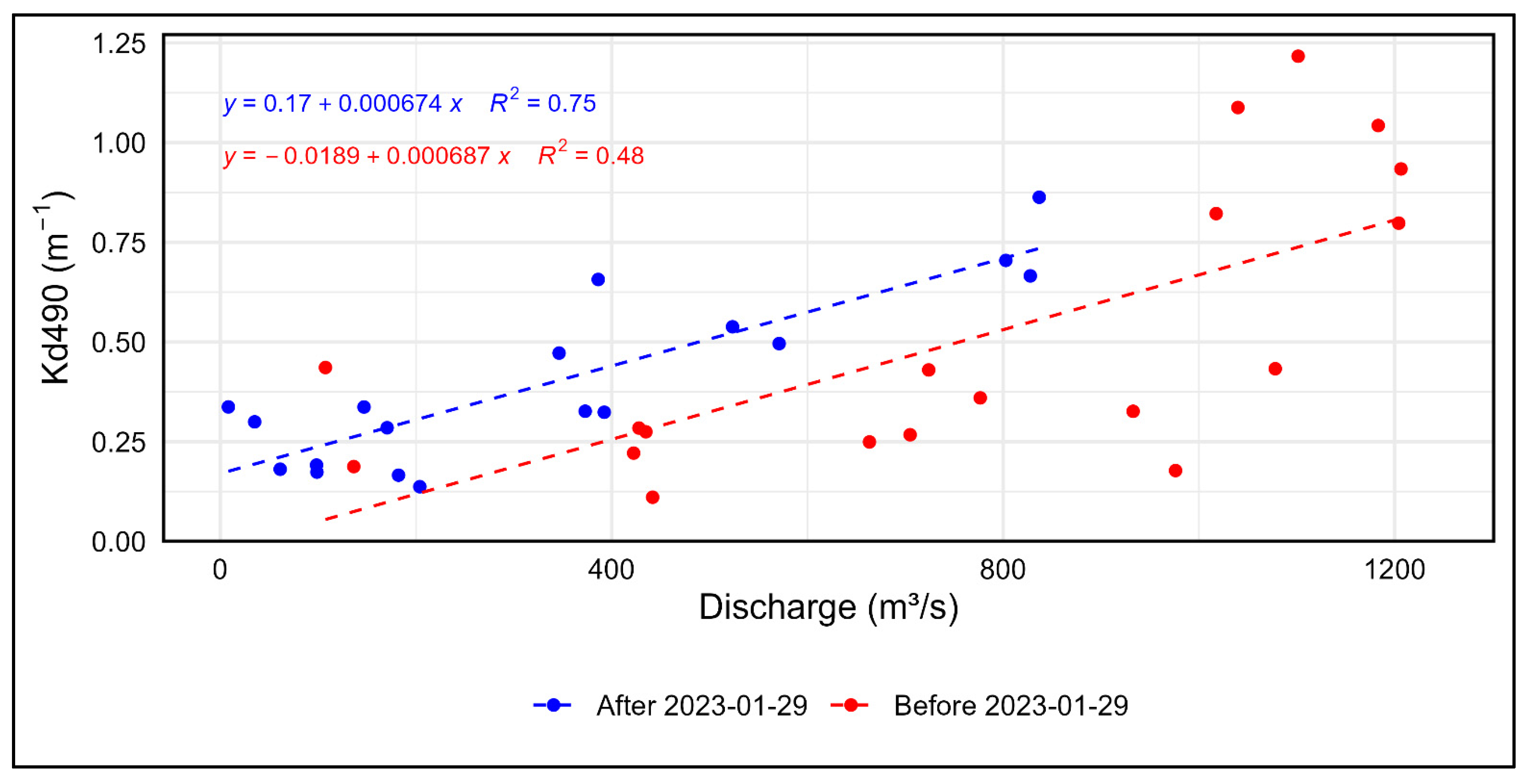
• This study highlights the significant role of riverine discharge in driving the surface sediment plume’s spatial extent and intensities, particularly within the plume’s inner core.
• The correlation observed between the Kd490 estimates and in situ turbidity data supports the utilisation of the Kd490 product in the future for sediment plume quantification within South Australian waters.
• These findings have important implications for environmental management. By revealing when and where plumes are likely to form and evolve, this study provides a foundation for targeted monitoring, timely management interventions, and informed planning to reduce the discussed ecological and socio-economic risks associated with extreme river discharge events.

6. Future Research

While this study provides important insights into the spatial and temporal dynamics of the River Murray sediment plume during the 2022–2023 flood event, several key areas warrant further investigation.

First, to strengthen validation and improve spatial resolution, future studies should incorporate higher-resolution satellite imagery. This would allow for more detailed observations of nearshore plume behaviour, particularly in dynamic environments where the MODIS resolution may be insufficient to capture finer-scale variability. Similarly, expanding the density and frequency of in situ sampling across a broader range of discharge stages would improve the capture of plume complexities and further support the validation of remotely sensed sediment indicators.

Furthermore, future research should aim to identify the primary drivers of plume dynamics under various combinations of typical driver behaviours in the region. Improved our understanding of the River Murray sediment plume’s temporal and spatial dynamics would support more effective riverine and coastal management strategies by informing predictive models and risk mitigation approaches aimed at reducing the impacts of sediment plumes on marine ecosystems and coastal communities.

References

1. Kudela, R.M.; Horner-Devine, A.R.; Banas, N.S.; Hickey, B.M.; Peterson, T.D.; McCabe, R.M.; Lessard, E.J.; Frame, E.; Bruland, K.W.; Jay, D.A. Multiple trophic levels fueled by recirculation in the Columbia River plume. Geophys. Res. Lett. 2010, 37, L18607. [Google Scholar] [CrossRef]
2. Yu, Y.Y.; Zhang, H.; Lemckert, C. Sediment transport in a shallow coastal region following severe flood events. Environ. Fluid Mech. 2017, 17, 1233–1253. [Google Scholar] [CrossRef]
3. Horner-Devine, A.R.; Hetland, R.D.; MacDonald, D.G. Mixing and transport in coastal river plumes. Annu. Rev. Fluid Mech. 2015, 47, 569–594. [Google Scholar] [CrossRef]
4. Aurin, D.; Mannino, A.; Franz, B. Spatially resolving ocean color and sediment dispersion in river plumes, coastal systems, and continental shelf waters. Remote Sens. Environ. 2013, 137, 212–225. [Google Scholar] [CrossRef]
5. Loisel, H.; Mangin, A.; Vantrepotte, V.; Dessailly, D.; Dinh, D.N.; Garnesson, P.; Ouillon, S.; Lefebvre, J.-P.; Mériaux, X.; Phan, T.M. Variability of suspended particulate matter concentration in coastal waters under the Mekong’s influence from ocean color (MERIS) remote sensing over the last decade. Remote Sens. Environ. 2014, 150, 218–230. [Google Scholar] [CrossRef]
6. Aufdenkampe, A.K.; Mayorga, E.; Raymond, P.A.; Melack, J.M.; Doney, S.C.; Alin, S.R.; Aalto, R.E.; Yoo, K. Riverine coupling of biogeochemical cycles between land, oceans, and atmosphere. Front. Ecol. Environ. 2011, 9, 53–60. [Google Scholar] [CrossRef]
7. Auricht, H.; Mosley, L.; Lewis, M.; Clarke, K. Mapping the long-term influence of river discharge on coastal ocean chlorophyll-a. Remote Sens. Ecol. Conserv. 2022, 8, 629–643. [Google Scholar] [CrossRef]
8. Bilotta, G.S.; Brazier, R.E. Understanding the influence of suspended solids on water quality and aquatic biota. Water Res. 2008, 42, 2849–2861. [Google Scholar] [CrossRef]
9. Hamidi, S.A.; Hosseiny, H.; Ekhtari, N.; Khazaei, B. Using MODIS remote sensing data for mapping the spatio-temporal variability of water quality and river turbid plume. J. Coast. Conserv. 2017, 21, 939–950. [Google Scholar] [CrossRef]
10. Fabricius, K.; Logan, M.; Weeks, S.; Lewis, S.; Brodie, J. Changes in water clarity in response to river discharges on the Great Barrier Reef continental shelf: 2002–2013. Estuar. Coast. Shelf Sci. 2016, 173, A1–A15. [Google Scholar] [CrossRef]
11. Storlazzi, C.D.; Norris, B.K.; Rosenberger, K.J. The influence of grain size, grain color, and suspended-sediment concentration on light attenuation: Why fine-grained terrestrial sediment is bad for coral reef ecosystems. Coral Reefs 2015, 34, 967–975. [Google Scholar] [CrossRef]
12. Wolanski, E.; Spagnol, S. Environmental degradation by mud in tropical estuaries. Reg. Environ. Chang. 2000, 1, 152–162. [Google Scholar] [CrossRef]
13. McLaughlin, C.; Smith, C.; Buddemeier, R.; Bartley, J.; Maxwell, B. Rivers, runoff, and reefs. Glob. Planet. Chang. 2003, 39, 191–199. [Google Scholar] [CrossRef]
14. Bainbridge, Z.T.; Wolanski, E.; Álvarez-Romero, J.G.; Lewis, S.E.; Brodie, J.E. Fine sediment and nutrient dynamics related to particle size and floc formation in a Burdekin River flood plume, Australia. Mar. Pollut. Bull. 2012, 65, 236–248. [Google Scholar] [CrossRef]
15. Petus, C.; Marieu, V.; Novoa, S.; Chust, G.; Bruneau, N.; Froidefond, J.-M. Monitoring spatio-temporal variability of the Adour River turbid plume (Bay of Biscay, France) with MODIS 250-m imagery. Cont. Shelf Res. 2014, 74, 35–49. [Google Scholar] [CrossRef]
16. Villas Bôas, A.B.; Ardhuin, F.; Ayet, A.; Bourassa, M.A.; Brandt, P.; Chapron, B.; Cornuelle, B.D.; Farrar, J.T.; Fewings, M.R.; Fox-Kemper, B. Integrated observations of global surface winds, currents, and waves: Requirements and challenges for the next decade. Front. Mar. Sci. 2019, 6, 425. [Google Scholar] [CrossRef]
17. Berdeal, I.G.; Hickey, B.; Kawase, M. Influence of Wind Stress and Ambient Flow on a High Discharge River Plume. J. Geophys. Res. Ocean. 2002, 107, 13-1–13-24. [Google Scholar]
18. Chant, R.J.; Wilkin, J.; Zhang, W.; Choi, B.-J.; Hunter, E.; Castelao, R.; Glenn, S.; Jurisa, J.; Schofield, O.; Houghton, R. Dispersal of the Hudson River plume in the New York Bight: Synthesis of observational and numerical studies during LaTTE. Oceanography 2008, 21, 148–161. [Google Scholar] [CrossRef]
19. Gong, W.; Wang, J.; Zhang, G.; Zhu, L. Effect of axial winds and waves on sediment dynamics in an idealized convergent partially mixed estuary. Mar. Geol. 2023, 458, 107015. [Google Scholar] [CrossRef]
20. Lisboa, P.V.; Fernandes, E.H.; Sottolichio, A.; Huybrecht, N.; Bendô, R. Coastal plumes contribution to the suspended sediment transport in the Southwest Atlantic inner continental shelf. J. Mar. Syst. 2022, 236, 103796. [Google Scholar] [CrossRef]
21. Sun, C. Riverine influence on ocean color in the equatorial South China Sea. Cont. Shelf Res. 2017, 143, 151–158. [Google Scholar] [CrossRef]
22. Valente, A.S.; da Silva, J.C. On the observability of the fortnightly cycle of the Tagus estuary turbid plume using MODIS ocean colour images. J. Mar. Syst. 2009, 75, 131–137. [Google Scholar] [CrossRef]
23. Verschelling, E.; van der Deijl, E.; van der Perk, M.; Sloff, K.; Middelkoop, H. Effects of discharge, wind, and tide on sedimentation in a recently restored tidal freshwater wetland. Hydrol. Process. 2017, 31, 2827–2841. [Google Scholar] [CrossRef]
24. Roth, M.K.; MacMahan, J.; Reniers, A.; Özgökmen, T.M.; Woodall, K.; Haus, B. Observations of inner shelf cross-shore surface material transport adjacent to a coastal inlet in the northern Gulf of Mexico. Cont. Shelf Res. 2017, 137, 142–153. [Google Scholar] [CrossRef]
25. Yang, G.; Wang, X.H.; Ritchie, E.A.; Qiao, L.; Li, G.; Cheng, Z. Using 250-M surface reflectance MODIS Aqua/Terra product to estimate turbidity in a macro-tidal harbour: Darwin Harbour, Australia. Remote Sens. 2018, 10, 997. [Google Scholar] [CrossRef]
26. Hickey, B.; Geier, S.; Kachel, N.; MacFadyen, A. A bi-directional river plume: The Columbia in summer. Cont. Shelf Res. 2005, 25, 1631–1656. [Google Scholar] [CrossRef]
27. Fong, D.A.; Geyer, W.R. The alongshore transport of freshwater in a surface-trapped river plume. J. Phys. Oceanogr. 2002, 32, 957–972. [Google Scholar] [CrossRef]
28. Bid, S.; Siddique, G. Identification of seasonal variation of water turbidity using NDTI method in Panchet Hill Dam, India. Model. Earth Syst. Environ. 2019, 5, 1179–1200. [Google Scholar] [CrossRef]
29. Fischer, A.M.; Pang, D.; Kidd, I.M.; Moreno-Madriñán, M.J. Spatio-temporal variability in a turbid and dynamic tidal estuarine environment (Tasmania, Australia): An assessment of MODIS band 1 reflectance. ISPRS Int. J. Geo-Inf. 2017, 6, 320. [Google Scholar] [CrossRef]
30. Dogliotti, A.I.; Ruddick, K.; Nechad, B.; Doxaran, D.; Knaeps, E. A single algorithm to retrieve turbidity from remotely-sensed data in all coastal and estuarine waters. Remote Sens. Environ. 2015, 156, 157–168. [Google Scholar] [CrossRef]
31. Moreno-Madrinan, M.J.; Al-Hamdan, M.Z.; Rickman, D.L.; Muller-Karger, F.E. Using the surface reflectance MODIS Terra product to estimate turbidity in Tampa Bay, Florida. Remote Sens. 2010, 2, 2713–2728. [Google Scholar] [CrossRef]
32. Doxaran, D.; Froidefond, J.-M.; Lavender, S.; Castaing, P. Spectral signature of highly turbid waters: Application with SPOT data to quantify suspended particulate matter concentrations. Remote Sens. Environ. 2002, 81, 149–161. [Google Scholar] [CrossRef]
33. Hu, C.; Chen, Z.; Clayton, T.D.; Swarzenski, P.; Brock, J.C.; Muller–Karger, F.E. Assessment of estuarine water-quality indicators using MODIS medium-resolution bands: Initial results from Tampa Bay, FL. Remote Sens. Environ. 2004, 93, 423–441. [Google Scholar] [CrossRef]
34. Gohin, F. Annual cycles of chlorophyll-a, non-algal suspended particulate matter, and turbidity observed from space and in-situ in coastal waters. Ocean Sci. 2011, 7, 705–732. [Google Scholar] [CrossRef]
35. Mueller, J.L. SeaWiFS algorithm for the diffuse attenuation coefficient, K (490), using water-leaving radiances at 490 and 555 nm. SeaWiFS Postlaunch Calibration Valid. Anal. Part 2000, 3, 24–27. [Google Scholar]
36. Diffuse Attenuation Coefficient for Downwelling Irradiance at 490 nm (Kd). Available online: https://oceancolor.gsfc.nasa.gov/resources/atbd/kd/#sec_2 (accessed on 16 May 2024).
37. Lei, S.; Xu, J.; Li, Y.; Lyu, H.; Liu, G.; Zheng, Z.; Xu, Y.; Du, C.; Zeng, S.; Wang, H. Temporal and spatial distribution of Kd (490) and its response to precipitation and wind in lake Hongze based on MODIS data. Ecol. Indic. 2020, 108, 105684. [Google Scholar] [CrossRef]
38. Wang, M.; Son, S.; Harding, L.W., Jr. Retrieval of diffuse attenuation coefficient in the Chesapeake Bay and turbid ocean regions for satellite ocean color applications. J. Geophys. Res. Ocean. 2009, 114. [Google Scholar] [CrossRef]
39. Zhang, T.; Fell, F. An empirical algorithm for determining the diffuse attenuation coefficient Kd in clear and turbid waters from spectral remote sensing reflectance. Limnol. Oceanogr. Methods 2007, 5, 457–462. [Google Scholar] [CrossRef]
40. Zhao, C.; Yu, D.; Yang, L.; Zhou, Y.; Gao, H.; Bian, X.; Li, Y. Remote sensing algorithms of seawater transparency: A review. In Proceedings of the 2022 3rd International Conference on Geology, Mapping and Remote Sensing (ICGMRS), Zhoushan, China, 22–24 April 2022; pp. 744–749. [Google Scholar]
41. Turbidity: Units of Measurement. Available online: https://or.water.usgs.gov/grapher/fnu.html (accessed on 16 May 2024).
42. Lee, Z.; Carder, K.L.; Arnone, R.A. Deriving inherent optical properties from water color: A multiband quasi-analytical algorithm for optically deep waters. Appl. Opt. 2002, 41, 5755–5772. [Google Scholar] [CrossRef]
43. Devlin, M.J.; Petus, C.; Da Silva, E.; Tracey, D.; Wolff, N.H.; Waterhouse, J.; Brodie, J. Water quality and river plume monitoring in the Great Barrier Reef: An overview of methods based on ocean colour satellite data. Remote Sens. 2015, 7, 12909–12941. [Google Scholar] [CrossRef]
44. Wang, J.; Wang, Y.; Lee, Z.; Wang, D.; Chen, S.; Lai, W. A revision of NASA SeaDAS atmospheric correction algorithm over turbid waters with artificial Neural Networks estimated remote-sensing reflectance in the near-infrared. ISPRS J. Photogramm. Remote Sens. 2022, 194, 235–249. [Google Scholar] [CrossRef]
45. Liu, Q.; Liu, D.; Zhu, X.; Zhou, Y.; Le, C.; Mao, Z.; Bai, J.; Bi, D.; Chen, P.; Chen, W. Optimum wavelength of spaceborne oceanic lidar in penetration depth. J. Quant. Spectrosc. Radiat. Transf. 2020, 256, 107310. [Google Scholar] [CrossRef]
46. Choo, J.; Cherukuru, N.; Lehmann, E.; Paget, M.; Mujahid, A.; Martin, P.; Müller, M. Spatial and temporal dynamics of suspended sediment concentrations in coastal waters of the South China Sea, off Sarawak, Borneo: Ocean colour remote sensing observations and analysis. Biogeosciences 2022, 19, 5837–5857. [Google Scholar] [CrossRef]
47. Doxaran, D.; Froidefond, J.-M.; Castaing, P.; Babin, M. Dynamics of the turbidity maximum zone in a macrotidal estuary (the Gironde, France): Observations from field and MODIS satellite data. Estuar. Coast. Shelf Sci. 2009, 81, 321–332. [Google Scholar] [CrossRef]
48. Petus, C.; da Silva, E.T.; Devlin, M.; Wenger, A.S.; Álvarez-Romero, J.G. Using MODIS data for mapping of water types within river plumes in the Great Barrier Reef, Australia: Towards the production of river plume risk maps for reef and seagrass ecosystems. J. Environ. Manag. 2014, 137, 163–177. [Google Scholar] [CrossRef]
49. 2022/2023 Flood Recovery Works. Available online: https://www.berribarmera.sa.gov.au/council-services/emergency/20222023-flood-recovery-works#:~:text=2022%2F2023%20River%20Murray%20Flood&text=This%20flood%20event%20was%20the,homes%2C%20shacks%20businesses%20and%20infrastructure (accessed on 16 May 2024).
50. 2022-23 River Murray Flood Event. Available online: https://www.environment.sa.gov.au/topics/river-murray-floods/2022-23-river-murray-flood-event (accessed on 14 November 2023).
51. River Murray Inundation Mapping. Available online: https://www.waterconnect.sa.gov.au/Systems/RMIM/SitePages/Home.aspx#:~:text=Historically%20this%20has%20occurred%20just,River%20Murray%20flood%20on%20record (accessed on 16 May 2024).
52. SA River Murray Flow Report: Report #50. Available online: https://www.waterconnect.sa.gov.au/Content/Flow%20Reports/RM-Flow-Report-2022%2012%2023_FINAL.pdf (accessed on 16 May 2024).
53. Murray-Darling Basin location. Available online: https://www.mdba.gov.au/basin/basin-location (accessed on 16 May 2024).
54. River Murray Estimated Travel Times during Flood Events. Available online: https://cdn.environment.sa.gov.au/environment/images/River-Murray-Estimated-Travel-Times.pdf (accessed on 16 May 2024).
55. River Murray Flows. Available online: https://www.environment.sa.gov.au/topics/river-murray-flows. (accessed on 16 May 2024).
56. Data Set: Discharge. Master—Daily Calculation—ML/day@A4261001. Available online: https://water.data.sa.gov.au/Data/DataSet/Summary/Location/A4261001/DataSet/Discharge/Master--Daily%20Calculation--ML%2Fday/Interval/Latest (accessed on 3 October 2024).
57. Leblanc, M.; Tweed, S.; Van Dijk, A.; Timbal, B. A review of historic and future hydrological changes in the Murray-Darling Basin. Glob. Planet. Chang. 2012, 80, 226–246. [Google Scholar] [CrossRef]
58. Dead Marine Life Washes onto South Coast Beaches Near Mouth of Flooding River Murray. Available online: https://www.abc.net.au/news/2023-01-06/carnage-of-dead-marine-life-on-beaches-near-murray-mouth/101831330 (accessed on 7 July 2023).
59. Geoscience Australia Sentinel-2A MSI Analysis Ready Data Collection 3—DEA Surface Reflectance (Sentinel-2A MSI), Scene ID: S2A_MSIL2A_20230101T004702. Geoscience Australia, Canberra. Available online: https://ecat.ga.gov.au/geonetwork/srv/eng/catalog.search#/metadata/146552 (accessed on 16 May 2024).
60. Ocean Color SMI: Standard Mapped Image MODIS Aqua Data. Available online: https://developers.google.com/earth-engine/datasets/catalog/NASA_OCEANDATA_MODIS-Aqua_L3SMI (accessed on 10 February 2024).
61. NASA Earth Data Level 3 & 4 Browser. Available online: https://oceancolor.gsfc.nasa.gov/l3/ (accessed on 10 February 2024).
62. Turbidity (Kd490), Maximum Monthly Climatological Mean (1998–2018), American Samoa. Available online: https://catalog.data.gov/dataset/turbidity-kd490-average-annual-frequency-of-anomalies-1998-2018-american-samoa (accessed on 16 April 2025).
63. Nukapothula, S.; Chen, C.; Yunus, A.P. Seasonal sediment plumes in the Krishna-Godavari basin using satellite observations. Deep Sea Res. Part I Oceanogr. Res. Pap. 2022, 188, 103850. [Google Scholar] [CrossRef]
64. Using the NASA Earth Data Level 3 Browser Interface. Available online: https://oceancolor.gsfc.nasa.gov/l3/help/ (accessed on 10 February 2024).
65. AusSeabed Marine Data Portal. Available online: https://portal.ga.gov.au/persona/marine (accessed on 27 February 2024).
66. Australian Bathymetry and Topography 250m 2023 (NEW). Available online: https://portal.ga.gov.au/metadata/elevation-and-depth/bathymetry-compilations/australian-bathymetry-and-topography-250m-2023-new-/13fd7f3c-7d54-4719-8aea-c69d00055742 (accessed on 10 February 2024).
67. Environmental, Economic and Social Values of the Encounter Marine Park, Department of Environment and Natural Resources, South Australia. Available online: https://cdn.environment.sa.gov.au/marineparks/docs/mp15.pdf (accessed on 16 May 2024).
68. Grzechnik, M.P. Three-dimensional tide and surge modelling and layered particle tracking techniques applied to Southern Australian coastal seas. Ph.D. Thesis, University of Adelaide, Adelaide, Australia, 2000. [Google Scholar]
69. “In-Situ Field Measurements for Adelaide Coastal Waters Study—Final Technical Report” ACWS Technical Report No. 7 Prepared for the Adelaide Coastal Waters Study Steering Committee. School of Chemistry, Physics and Earth Sciences, Flinders University of SA. Adelaide. Available online: https://www.epa.sa.gov.au/files/477441_acws7.pdf (accessed on 16 May 2024).
70. Karimaee Tabarestani, M.; Zarrati, A. Sediment transport during flood event: A review. Int. J. Environ. Sci. Technol. 2015, 12, 775–788. [Google Scholar] [CrossRef]
71. Xing, J.; Davies, A.M. The effect of wind direction and mixing upon the spreading of a buoyant plume in a non-tidal regime. Cont. Shelf Res. 1999, 19, 1437–1483. [Google Scholar] [CrossRef]
72. Wright, L.D. Sediment transport and deposition at river mouths: A synthesis. Geol. Soc. Am. Bull. 1977, 88, 857–868. [Google Scholar] [CrossRef]
73. Kostaschuk, R.A.; Stephan, B.A.; Luternauer, J.L. Suspended sediment concentration in a bouyant plume: Fraser River, Canada. Geo-Mar. Lett. 1993, 13, 165–171. [Google Scholar] [CrossRef]
74. Warrick, J.A.; Mertes, L.A.; Washburn, L.; Siegel, D.A. A conceptual model for river water and sediment dispersal in the Santa Barbara Channel, California. Cont. Shelf Res. 2004, 24, 2029–2043. [Google Scholar] [CrossRef]
75. Pak, H.; Zaneveld, J.; Spinrad, R. Vertical distribution of suspended particulate matter in the Zaire river, estuary and plume. Neth. J. Sea Res. 1984, 17, 412–425. [Google Scholar] [CrossRef]
76. Rao, Y.R.; Schwab, D.J. Transport and mixing between the coastal and offshore waters in the Great Lakes: A review. J. Great Lakes Res. 2007, 33, 202–218. [Google Scholar] [CrossRef]
77. Hill, P.S.; Milligan, T.G.; Geyer, W.R. Controls on effective settling velocity of suspended sediment in the Eel River flood plume. Cont. Shelf Res. 2000, 20, 2095–2111. [Google Scholar] [CrossRef]
78. Mertes, L.A.; Smith, M.O.; Adams, J.B. Estimating suspended sediment concentrations in surface waters of the Amazon River wetlands from Landsat images. Remote Sens. Environ. 1993, 43, 281–301. [Google Scholar] [CrossRef]
Figure 1. (a) A map illustrating the Murray–Darling Basin (MDB) relative to Australia and the River Murray. (b) A map illustrating the Lower Lakes of the River Murray, the Murray Mouth, and locations of interest in the surrounding coastal zone. The Murray–Darling Basin shape file was downloaded from https://data.gov.au/data/dataset/murray-darling-basin-boundary (accessed 1 June 2024). River Murray shape file was downloaded from https://www.waterconnect.sa.gov.au/Systems/SitePages/Spatial%20Data.aspx (accessed 2 June 2024). The delineated Murray Mouth zone is characterised by being within 10 km of the Murray Mouth and with a bathymetry less than 30 m deep.
Remotesensing 17 01711 g001
Figure 2. River Murray flow rates at the SA/VIC border from 1977 to 2024, with DEW-defined flow thresholds illustrated [56].
Remotesensing 17 01711 g002
Figure 3. Surface reflectance true colour imagery, contrast-stretched, captured by a Sentinel-2 sensor in the northern part of Long Bay amidst the peak flood discharge, 1 January 2023 [59].
Remotesensing 17 01711 g003
Figure 4. A closer view of a portion of the flood plume on the 6 January 2023, illustrating the distinct boundary between the plume and the surrounding coastal waters [59].
Remotesensing 17 01711 g004
Figure 5. River Murray flow rates at the SA/VIC border across 2022, with the DEW-defined high flow threshold and 1 July 2022 illustrated [56].
Remotesensing 17 01711 g005
Figure 6. Barrage locations within the Lower Lakes. The barrages are utilised to restrict the movement of seawater into the freshwater systems of the lakes and upriver.
Remotesensing 17 01711 g006
Figure 7. The spatial extent where Equation (1) was applied (137, 140, −37, −35). The delineated Murray Mouth zone is also illustrated to highlight the spatial variation between the two.
Remotesensing 17 01711 g007
Figure 8. Locations of conductivity, temperature, and depth (CTD) casts during the high riverine discharge measurement period (2123 February 2023).
Remotesensing 17 01711 g008
Figure 9. Locations of CTD casts during the post-flood event measurement period (31 May–1 June 2023).
Remotesensing 17 01711 g009
Figure 10. (a) The total daily riverine discharge calculated from the 5 barrage locations (Figure 6). (b) The significant Kd490 area across the flood event. (c) The median Kd490 at the Murray Mouth across the flood event. Each point is coloured relative to the number of pixels used in the median calculation, and the reference Kd490 range is plotted to a 90% confidence interval, between the 5th and 95th percentile of reference zonal data.
Remotesensing 17 01711 g010
Figure 11. Relationship between significant Kd490 area and total riverine discharge (1 August 2022 to 30 June 2023), showing that plume area increases as total discharge increases. Data are split into two subsets based on their relation to date of peak discharge on 29 January 2023, with points coloured accordingly to distinguish between pre- and post-peak conditions.
Remotesensing 17 01711 g011
Figure 12. The relationship between the median Kd490 at the Murray Mouth and the total riverine discharge (1 August 2022 to 30 June 2023), showing that the water quality decreases as the total discharge increases. Data are split into two subsets based on their relation to the date of peak discharge on 29 January 2023, with points coloured accordingly to distinguish between pre- and post-peak conditions.
Remotesensing 17 01711 g012
Figure 13. Visualisations of Kd490 estimates in “weekly” panels to illustrate the temporal and spatial distribution of Kd490 estimates across the flood event (1 November 2022 to 6 April 2023). The date printed above each panel represents day 1 of the 8-day composition period. Data for the entire assessment period (1 August 2022 to 30 June 2023) are included in Appendix A.
Remotesensing 17 01711 g013
Figure 14. Visualisations of sediment plume presence (significant Kd490 estimates) in “weekly” panels to illustrate the temporal and spatial distribution of the sediment plume across the flood event (1 November 2022 to 6 April 2023). The date printed above each panel represents day 1 of the 8-day composition period. Data for the entire assessment period (1 August 2022 to 30 June 2023) are included in Appendix B.
Remotesensing 17 01711 g014
Figure 15. The relationship between turbidity and the distance from the mouth during two periods in 2023: (1) February during high riverine discharge (21 February 2023 to 23 February 2023) and (2) May–June, the post-flood event (31 May 2023 to 1 June 2023). In February, the turbidity generally decreases with the distance from the mouth. In contrast, post-flood data show divergent patterns by depth: the turbidity at 2 m depth slightly increases with distance, while the turbidity at 3 m depth decreases.
Remotesensing 17 01711 g015
Figure 16. Relationship between turbidity and Kd490 during two survey periods in 2023: (1) February during high riverine discharge (turbidity data: 21 February 2023 to 23 February 2023; Kd490: 18 February 2023 to 25 February 2023) and (2) May–June post-flood event (turbidity data: 31 May 2023 to 1 June 2023; Kd490: 5 May 2023 to 1 June 2023). During high discharge, turbidity increases with Kd490 values. In contrast, post-flood data show depth-dependent patterns: turbidity at 3 m depth increases with Kd490, while turbidity at 2 m depth decreases.
Remotesensing 17 01711 g016
Figure 17. The temporal distribution of the sentinel-2 satellite imagery and sediment plume positions (from Figure 14) relative to the riverine discharge data (1 October 2022 to 30 April 2023). (A) Riverine discharge at the Murray Mouth with typical and distinct plume positions of B1, B2, and C indicated by red vertical date markers. (B) True colour imagery accessed through the Google Earth Engine, composited from all scenes acquired from 1 November 2022 to 14 November 2022 (B1) and from 17 December 2022 to 18 December 2022 (B2), stretched to two standard deviations, to enhance visual plume identification. (C) Kd490 estimates from 17 January 2023 to 17 February 2023, with the date above each panel representing day 1 of the 8-day composition period.
Remotesensing 17 01711 g017