Article

Detection of Small-Scale Subsurface Echoes Using Lunar Radar Sounder and Surface Scattering Simulations with a DEM Generated Using a Generative Adversarial Network

1
Department of Space and Astronautical Science, The Graduate University for Advanced Studies, SOKENDAI, Sagamihara 252-5210, Kanagawa, Japan
2
Institute of Space and Astronautical Science, Japan Aerospace Exploration Agency (JAXA), Sagamihara 252-5210, Kanagawa, Japan
3
Institute for Radioastronomy, National Institute for Astrophysics (INAF), Via Piero Gobetti 101, 40129 Bologna, Italy
4
Graduate School of Science, Tohoku University, Sendai 980-8578, Miyagi, Japan
5
Department of Earth, Environmental and Planetary Sciences, Brown University, Providence, RI 02912, USA
*
Author to whom correspondence should be addressed.
Remote Sens. 2025, 17(10), 1710; https://doi.org/10.3390/rs17101710
Submission received: 24 March 2025 / Revised: 7 May 2025 / Accepted: 10 May 2025 / Published: 13 May 2025

Abstract

:
Spaceborne radar is a powerful tool for probing planetary subsurface structures. Earlier radar studies of the Moon have primarily examined large-scale horizontal structures. However, recent discoveries of vertical holes suggesting the existence of lava tubes and theoretically predicted subsurface gas voids formed by volatiles in magma have highlighted the importance of small-scale subsurface structures. We developed a method using SELENE Lunar Radar Sounder (LRS) data to detect small-scale subsurface echoes (hundreds of meters). Surface scattering simulations incorporating incoherent scattering from sub-resolution roughness were performed using a high-resolution digital elevation model generated by a generative adversarial network. Detection thresholds for subsurface echo candidates (SECs) were determined from the histograms of difference intensities between LRS and simulation B-scans. Results show that some SECs exist in the extension area of the analyzed graben. SECs were also detected continuously across multiple LRS ground tracks in areas unrelated to grabens. Using the radar equation analysis, the echo intensities of SECs could be explained for subsurface structures with 50–600 m widths and dielectric constants of 1–4. This suggests the existence of either subsurface voids or materials with a high porosity of more than 35%. Among the SECs detected continuously across multiple LRS ground tracks, those that are more or less aligned in the downward elevation direction are likely indicative of lava tubes. On the other hand, the SECs distributed along the extension of the graben are aligned parallel to the contour lines. These SECs likely suggest gas voids at the tip of the intrusive magma that formed the graben.

1. Introduction

Subsurface structures of planets reflect their past volcanic and tectonic activity. Detailed understanding of subsurface structures is therefore important for elucidating a planet’s geological evolution and thermal environment from its formation to the present.
Spaceborne radar is a powerful tool for investigating subsurface structures. Such instruments actively transmit electromagnetic waves and receive their reflections from the surface and subsurface, enabling subsurface characterization. On Mars, subsurface ice and candidate liquid water layers were discovered by Mars Advanced Radar for Subsurface and Ionospheric Sounding (MARSIS) on Mars Express and Shallow Radar (SHARAD) launched with the Mars Reconnaissance Orbiter [1,2,3]. On the Moon, the Lunar Radar Sounder (LRS) onboard Selenological and Engineering Explorer (SELENE) first detected reflection echoes from regolith layers located several hundred meters beneath the surface, formed between different lava layers [4]. These LRS echoes have been mapped across the entire lunar mare regions, enabling the estimation of the volumes and rates of lava eruptions occurring before and after the formation of each regolith layer [5,6,7]. These LRS subsurface echoes are also useful for estimating the material properties of the uppermost basalt layers to depths of a few hundred meters. The bulk dielectric constant and porosity of the overlying deposits have been estimated by analyzing the time delay between the surface and subsurface echoes in combination with the excavation depths of nearby craters [8]. Independently of the method described above, dielectric constant, porosity, and loss tangent values that can explain the strengths of the LRS subsurface echoes have been estimated using the radar range equation [9]. The LRS is also used for shallow subsurface structures at depths of several tens of meters. Kobayashi et al. (2010) [10] showed that, if a boundary exists between the surface regolith and an underlying lava flow at shallow depths, the reflection from this boundary can overlap with the surface reflection, causing the observed surface range to appear deeper than the actual surface (range extension). They further identified such range extensions in actual LRS data and used them to estimate the surface regolith layer thickness. Most radar surveys have examined large-scale horizontal subsurface structures ranging from tens to hundreds of kilometers. These reflected echoes, which were detected continuously over a large horizontal area, had strong echo intensity, making them detectable by visual analysis of the radargrams or by a simple analytical method that reduces surface scattering by stacking multiple radargrams.
Recently, detection of small-scale subsurface structures (hundreds of meters to several kilometers) on the Moon has become increasingly important. A theoretical study of lunar magma ascent has suggested that magma rise is driven by buoyancy and the exsolution of volatiles. If the magma fails to erupt, then gas voids form at the magma tip [11]. These voids are likely to become empty voids as the gas escapes over time through microfractures. In addition, numerous irregular mare patches (IMPs) have been discovered in recent years [12,13]. Reportedly, they are formed by volcanic eruptions containing volatiles within magma. Beneath the IMPs, porous rocks formed by the foaming of volatiles might be present [12,13]. Consequently, detecting the subsurface gas voids and porous rocks provides evidence of volatiles within lunar magma. Moreover, lava tubes predicted on the Moon are candidate sites for future human habitation in terms of radiation shielding and thermal stability. Therefore, detecting such subsurface voids is necessary for selecting suitable locations for future bases [14]. To date, several studies have emphasized the detection of such small-scale subsurface structures on the Moon using LRS data. Kaku et al. (2017) [15] discovered non-reflective areas below −25 dB and secondary echo peaks, both occurring following the surface echoes. These echo patterns appear as point-like reflections spanning one or two pixels in the along-track direction of the spacecraft [15]. These echoes correspond to mass-deficit regions of the GRAIL gravity data [16,17], suggesting the existence of lava tubes. However, although LRS data include scattered signals not only from nadir subsurface structures but also from off-nadir surfaces, the surface scattering effects have not been evaluated sufficiently in this study. Furthermore, considering the LRS footprint, Kobayashi et al. (2020) [18] showed that reflected echoes from the lava tube should be detected at least eight consecutive points in the latitudinal direction instead of a point-like echo. Donini et al. (2020) [19] introduced an unsupervised fuzzy system for detecting candidate lava tubes from lunar radar sounder (LRS) data. This approach models the electromagnetic and geometric properties of lava tubes to identify characteristic reflections in radargrams (reflection intensity, phase inversion, etc.). The method was validated using LRS data of the Marius Hills region and successfully extracted some candidate lava tube echoes reported by Kaku et al. (2017) [15] in a completely automatic way. However, this study was limited to characterizing the surface scattering echoes from a simplified lunar surface with a few craters, with no detailed evaluation of surface scattering from the actual complex lunar surface.
Kobayashi et al. (2020) [18] simulated surface scattering in detail using the method based on the Stratton–Chu integral. They pointed out that the echoes found from the earlier study [15] were likely to be attributable to surface scattering. However, the intensities of the simulation results presented by Kobayashi et al. (2020) [18] are generally higher than those of the LRS data at depths greater than 500 m, which might be attributable to artifactual topography included in the digital elevation model (DEM) that was used. For more accurate surface scattering simulations, a higher-resolution DEM than the previously used SLDEM2015 [20] is necessary. NACDEM has the highest resolution on the Moon (2–5 m/pixel) [21], but NACDEM cannot be used for surface scattering simulations that require a DEM that covers at least a 1° circular area centered on the LRS observation point because of its limited longitudinal coverage. A DEM with both NACDEM-level high resolution and wide coverage must be developed for more accurate surface scattering simulations. Traditionally, lunar DEMs have been generated by stereo photogrammetry using image pairs acquired at different viewing angles [22,23]. However, stereo-based methods suffer from reduced accuracy in areas with poor stereo geometry or low image contrast, resulting in DEMs with resolutions approximately three times coarser than the stereo imagery [21]. Shape-from-shading (SFS) techniques have been developed to reconstruct pixel-scale DEMs from the shading information in a single image, assuming illumination conditions and surface reflectance properties [21]. Because high-resolution optical images acquired by LRO NAC are available for almost the entire lunar surface, it is possible to generate higher-resolution DEMs globally using SFS than those produced using stereo photogrammetry. However, it is sensitive to albedo variations and assumptions of surface reflectance properties, which often engender ambiguities and inaccuracies in complex terrains. Recent advances in deep learning have led to the development of convolutional neural network (CNN)-based approaches for DEM generation. In CNN-based models, optical images and low-resolution DEMs are used as inputs to learn the relationship between absolute elevation values and optical conditions, enabling the generation of high-resolution DEMs. These approaches have been applied to Mars, successfully producing DEMs with higher resolution than that obtained by traditional stereo imaging [22]. However, CNN-based methods tend to generate smoothed topography because of the large receptive fields used for regularization [23]. To solve this issue, CNN-based DEMs are used as inputs to shape-from-shading (SFS), improving the reconstruction accuracy of high-frequency terrain [24]. However, because this approach still relies on SFS, it remains fundamentally affected by differences in optical conditions, making it unsuitable for generating high-precision and spatially consistent DEMs over wide areas. Generative adversarial network (GAN) has also been proposed as a deep learning approach for DEM generation. GAN consists of a generator that creates fake images from optical images and low-resolution DEMs and a discriminator that evaluates the authenticity of their generated DEMs. Through adversarial training between these two models, a model capable of generating high-resolution DEMs can be constructed. Liu et al. (2022) [25] generated a high-precision DEM of the lunar surface using GAN and showed that the reconstruction results can be consistent even when optical images taken at different solar altitude angles are used as input. This finding demonstrates that GAN can generate a high-precision DEM that is independent of differences in the lighting conditions of images.
Another possibility that might cause relatively high-intensity echoes in the LRS data is small-scale roughness less than the resolution of the DEM. Gerekos et al. (2023) [26] evaluated the effect of incoherent scattering, which had not been considered in earlier simulations, by approximating the surface with square cells and by assuming that the cells have small-scale roughness with root mean square (RMS) height and correlation length. The results obtained when applying this method to LRS data in the Oceanus Procellarum region of the Moon demonstrated that when considering roughness with an RMS height of 1.5 m and a correlation length of 70 m, the simulation result approached the radargram of the LRS observation data. Therefore, accurate assessment of incoherent scattering from roughness smaller than the cell size must be achieved to enhance subsurface echo detection.
For this study, to detect small-scale subsurface echoes from the LRS, we first use GAN to generate a high-precision DEM required for high-precision surface scattering simulation. The use of this technique reduces artifactual topography, which has previously degraded the accuracy of surface scattering simulations. Additionally, we incorporate the method proposed in an earlier study [26] in a surface scattering simulation and then consider the effects of incoherent scattering caused by sub-cell roughness. The LRS B-scan and simulation B-scan are downsampled to the LRS resolution range. Furthermore, a detection threshold for subsurface echoes is determined from the histogram of their differences, extracting subsurface echoes. Finally, we analyze the spatial distribution of subsurface echoes and evaluate the reliability of small-scale subsurface echo detection and the subsurface structure indicated by the detected subsurface echoes.

2. Materials and Methods

To extract small-scale subsurface echoes with hundreds of meters, which is close to the LRS azimuth resolution, from LRS data, we perform three main processes: generation of a high-resolution DEM using a GAN, surface scattering simulation, and detection of subsurface echoes. Figure 1 shows the overall process of the proposed approach. In the DEM generation phase, we construct a GAN model using high-resolution images (LRONAC images), a low-resolution DEM (SLDEM2015), and a high-resolution DEM (NACDEM). Then this model is then used to generate high-resolution DEMs by inputting SLDEM2015 and LRONAC images in areas where NACDEM does not exist. In the surface scattering simulation phase, we calculate the electromagnetic field scattered from the lunar surface using the high-resolution DEM generated by the GAN. Incoherent scattering caused by roughness less than the resolution of the DEM is implemented based on a method proposed in an earlier study [26]. Finally, by comparing the results of the surface scattering simulation with the LRS observation data, we identify small-scale subsurface echoes that might indicate lava tubes and volatile gas voids.

2.1. Generation of a High-Resolution DEM Using a GAN

The DEM accuracy strongly affects the surface scattering simulation accuracy. Ideally, a DEM with resolution that is 1/10 of the observation wavelength is required to acquire accurate simulation results [27]. To create a DEM with higher accuracy than SLDEM2015, we generate a DEM using a GAN proposed in an earlier report [25]. This GAN consists of two models: a generator that generates fake images from high-resolution images (LRONAC images) and a low-resolution DEM (SLDEM2015) and a discriminator that distinguishes between fake images and truth images (NACDEM). The generator learns to create fake images that resemble the truth images, whereas the discriminator learns to distinguish truth images from fake images accurately. Through this adversarial learning process, the two models learn collectively to generate images close to NACDEM. Finally, by inputting LRONAC images and SLDEM into this model in areas where NACDEM does not exist, a high-resolution DEM can be generated (hereinafter designated as GANDEM). The architectures, loss functions, and parameters used for the generator and discriminator are adopted from those proposed in an earlier report (see [25] and Supplementary Materials, Text S1). As in that earlier study, the three input data to the GAN model are input uniformly at 10 m/pixel. Therefore, GANDEM is output at 10 m/pixel.

2.2. Surface Scattering Simulation

The LRS data include both surface-scattered echoes and subsurface echoes. To estimate surface-scattered echoes within the LRS data, we simulate the surface scattering of LRS electromagnetic waves. The scattered electric field E s at the satellite receiving point is calculable by solving the following Stratton–Chu integral for monostatic radar.
E s r r , ω = S i k 1 4 π r r r · e i k r r r · I ̿ k ^ s k ^ s η n ^ × H r , ω + k ^ s × n ^ × E r , ω · d A r
Therein, r r and r , respectively, signify the position vector of the receiving antenna and that of an arbitrary surface. i indicate imaginary unit. In addition, ω and k , respectively, denote the LRS angular frequency and wavenumber. Also, I ̿ is a unit tensor. k ^ s is the direction vector from the surface to the receiving antenna. η = μ ε represents the characteristic impedance. n ^ denote normal vector of the cell. H and E , respectively, represent magnetic and electric fields. d A denotes a small area of an arbitrary surface. S stands for the total lunar surface to be integrated. For numerical calculations, the lunar surface is approximated by rectangular cells using GANDEM; Equation (1) can be rewritten as presented below.
E s r r , ω = i k α = 1 N 1 4 π r r r α I ̿ k ^ s k ^ s · η n ^ × H r α , ω + k ^ s × n ^ × E r α , ω · S e 2 i k r r r d Σ
In that equation, r α is the position vector of a cell represented by the index α ; d Σ denotes the area of a cell. N is the total number of cells. Although GANDEM is originally a 10 m/pixel dataset as described in Section 2.1, it is downsampled to 60 m/pixel for use in surface scattering simulations. As shown in Supplementary Materials Text S2, the simulation results using the original GANDEM and the DEMs resampled to 30 m/pixel and 60 m/pixel are nearly identical. Therefore, we chose to use the 60 m/pixel data to improve computational efficiency.
Equation (2) is based on the assumption that each cell is flat. It does not include the effect of small-scale roughness less than the cell size. To account for incoherent scattering from roughness with correlation lengths smaller than the GANDEM cell size (i.e., less than 60 m), we transform Equation (2) into the following equations based on the method used for an earlier study [26]. Then we calculate the coherent and incoherent components of the reflected electric field separately as shown below.
E t o t r r ,   ω = E c o h r r ,   ω + E i n c o h r r ,   ω
E c o h r r ,   ω = α N F α r α , r r ϕ ~ α r α , r r
E i n c o h r r ,   ω = α N F α r α , r r D ϕ ,   α r α , r r   e 2 k r α r r e ϕ r
F α r α , r r = i k I k ^ s k ^ s 4 π r r r α · η n ^ × H r α , ω + k ^ s × n ^ × E r α , ω
In those equations, E c o h , E i n c o h , and E t o t , respectively, denote coherent and incoherent components of a reflected electromagnetic field, as well as the total electromagnetic field. Also, ϕ ~ α is the phase of a reflected signal from the small area in the cell with index α. ϕ r denotes a random phase caused by incoherent scattering and are defined by ϕ r = a + b i 2 , where a ,   b   ~   N ( 0,1 ) . ϕ ~ α and D ϕ ,   α are variables determined by the RMS height σ R M S and the correlation coefficient l of random roughness [26].
The surface-scattered electromagnetic field received by the LRS is the inner product of E t o t in Equation (3) and the unit vector parallel to the antenna element ( L ^ ). Inverse-Fourier transformation of the product of this inner product ( E t o t r r , ω · L ^ ) and the frequency response of the LRS transmitted signal ( F ω ) is performed to obtain the LRS surface-scattered signal in the time domain.
E r t = 1 2 π F ω E t o t r r ,   ω · L ^ e i ω t d ω
Finally, by application of range compression processing [28] and SAR processing [29] to E r , simulation data are generated for comparison with SELENE LRS data.

2.3. SELENE LRS Data

The LRS transmits a linear up-chirp signal (a signal whose frequency increases linearly over time) at 4–6 MHz, with a 50 msec interval, from a nominal altitude of 100 km; it receives echoes from both the lunar surface and subsurface [28]. The received signal is multiplied by a reference signal onboard. It is then Fourier transformed (equivalent to range compression), resulting in a theoretical range resolution of 75 m [28] and applied with synthetic aperture radar (SAR) processing with a synthetic aperture range of 5 km [29], which improves the resolution in the spacecraft movement direction to 600 m. For this study, we perform this SAR processing assuming that the signal travels through a single uniform medium with the same dielectric properties as a vacuum.

2.4. Detection of Subsurface Echoes

The two-dimensional echo profile, designated as a B-scan, has vertical and horizontal axes with the apparent depth (assuming a dielectric constant of 1 for the subsurface medium) and the spacecraft movement direction (almost corresponding to the latitude). For this study, B-scans obtained from the SELENE LRS data and surface scattering simulation data (Section 2.2) are defined, respectively, as the observation B-scan and the simulation B-scan. The reflection intensity of each B-scan is normalized so that the strongest intensity is 0 dB. The subsurface signals within the LRS data are extracted through the following six steps using two B-scans.
Step I. Surface scattering simulation is performed for LRS data in the research area.
Step II. B-scans are created by averaging the original B-scans with larger pixels of 600 m/pixel in the horizontal direction and 100 m/pixel in the depth direction.
Step III. Pixels with intensities higher than the effective noise level (−25 dB) of the LRS data used for this study [15] are extracted from the averaged observation B-scan.
Step IV. For the pixels extracted in Step III, the intensity difference between the pixel at the same location and the eight surrounding pixels in the averaged simulation B-scan is calculated as
d I = min m , n i 1 , i , i + 1 , { j 1 , j , j + 1 } I o b s i , j I s i m ( m , n )
where I o b s and I s i m , respectively, represent the intensities in an averaged observation B-scan and an averaged simulation B-scan. Also, i and j , respectively, represent the depth and horizontal index in the two B-scans. Among the nine intensity difference values, the smallest value is set as the intensity difference ( d I ( i , j ) ) at the corresponding position.
Step V. A histogram of the difference d I obtained in Step IV is generated and separated into a normal distribution with a mean of 0 and other components using a Gaussian mixture model (GMM), a machine learning method that classifies data by estimating the probability that each datum belongs to a Gaussian distribution [30]. The 3σ line of the identified normal distribution with a mean of 0 is set as the subsurface echo detection threshold.
Step VI. For given LRS data, the processes from Step I to Step V are performed 10 times with different random phases ϕ r in Equation (5). Pixels P ( i , j ) that exceed the subsurface echo detection threshold in all 10 times are extracted.
Herein, we refer to pixels obtained after these six steps as subsurface echo candidates (SECs). The pixel size of the averaged B-scan in STEP II is determined by the horizontal resolution in the spacecraft movement direction [29] and the effective range resolution in the depth direction [28]. The effective noise level of STEP III is based on an earlier study [15]. STEP IV is performed considering the potential horizontal and depth misalignment of surface scattering echoes between the LRS observation B-scan and simulation B-scan because of orbital errors of LRS and spatial errors in SLDEM2015. The orbital errors of SELENE are primarily caused by limitations in the lunar gravity field model and deviations from the predicted orbital trajectory after the attitude control event, resulting in cross-track and along-track deviations on the order of several tens of meters [31]. In Step VI, the surface scattering simulation is performed 10 times to detect subsurface echoes. Conducting only a single simulation is likely to result in a high false detection rate because the surface scattering simulation incorporates random phase variations, as described in Equation (5). Therefore, ten simulations are performed using the same observed LRS data. Only those pixels that satisfy the Step V criteria in all ten simulations are extracted as SECs. This method enables the extraction of subsurface echoes with a reduced false detection rate.

2.5. Estimation of Subsurface Echo Intensity Using the Radar Equation

Using radar equations, we investigate subsurface echo intensities to estimate the presence of subsurface void structures. For this study, the reflected echo intensity from the tip of a subsurface intrusive dike is analyzed (Figure 2). Based on the method developed for an earlier study [18], the relative intensity of the reflected echo from the subsurface to that from the nadir surface ( I s u b / s u r ) is calculated as shown below.
        I s u b / s u r = 10 l o g 10 A s u b A s u r + 10 l o g 10 R s u b 2 R s u r 2
R sur = R 01   ,               R sur =   T 01 R 12 T 10
  R 01 = ε 0 ε 1 ε 0 + ε 1   ,   T 01 = 2 ε 1 ε 0 + ε 1 ,   R 12 = ε 1 ε 2 ε 1 + ε 2   ,   T 10 = 2 ε 0 ε 0 + ε 1
In those equations, A s u r and A s u b , respectively, represent the radar-illuminated areas of the surface and the subsurface. A s u r is calculated by multiplying the LRS resolution along the satellite track of 600 m by the surface illumination distance along the cross-track direction of 3500 m [18]. A s u b is calculated by multiplying the dike width by the surface illumination distance in the cross-track direction. Reflection coefficient R and transmission coefficient T are calculated based on the Fresnel model. Two-digit subscripts show that the electromagnetic wave propagates from the medium with the first subscript to the medium with the second subscript. In addition, ε 0 , ε 1 , and ε 2 , respectively, stand for the dielectric constants of vacuum, the host basalt, and the dike-tip material. The lunar dielectric constant can be expressed as a function of the FeO and TiO2 contents in units of wt.% and the porosity (P) [32].
ε = 1.919 ρ
  ρ = 1 P · ρ 0    
ρ 0 = 0.0273 · F e O + 0.0110 · T i O 2 + 2.773  
In those equations, ρ stands for the material density with assumed porosity, and ρ 0 represents the true density, which is the density of a material with assumed porosity of 0. The attenuation rate ( γ ) for the LRS electromagnetic waves passing through lunar basalt can be estimated as shown below [33,34].
  γ = 0.091 · ε · f c · t a n δ   [ d B / m ]
  t a n δ = 5.3 × 10 4 ± 5.6 × 10 4 + 2.5 × 10 4 ± 9 × 10 5 · C · ρ
    C = F e O + T i O 2        
In those equations, f c denotes the LRS central frequency in units of megahertz and C represents the sum of FeO and TiO2 contents. Consequently, when the LRS electromagnetic wave passes through distance D m in the material with ε 1 , the subsurface reflection intensity including attenuation ( I s u b / s u r ’) is expressed as presented below.
I s u b / s u r = I s u b / s u r 2   γ D

2.6. Geological Characteristics of the Analyzed Region

The Cauchy region, located in the eastern Mare Tranquillitatis, has an elevation higher than that of the western side (Figure 3a,b). It is noteworthy that it has a low-density anorthosite crustal thickness of up to 50 km [35,36], which is considerably thicker than typical crustal thicknesses of the nearside maria regions (Figure 3c). In addition, the region has few radioactive elements [37,38] that promote increased magma temperature and consequently decreased magma density (Figure 3d). Under such conditions, magma becomes stagnant within the crust, which likely leads to the formation of subsurface gas voids at magma tips because of volatiles within the magma (see Supplementary Materials Text S3).
In the Cauchy region, we select as the analyzed region an area (8.4–9.8°N, 32.0–34.0°E; shown by the frames in Figure 4a,b) with multiple linear grabens (shown by white dashed lines in Figure 4a). Theoretical studies and terrestrial observations have shown that a graben forms when magma intrudes into the shallow subsurface [39]. This finding suggests subsurface magmatic intrusions at shallow depth exist in the area surrounding the graben. In the analyzed region, the crustal thickness is 36–50 km (average 43 km). The thorium content is less than 2 ppm, with typical characteristics of the Cauchy region. Therefore, this analyzed region is suitable for investigating the possible presence of gas voids located at the stalled magmatic dike tips.
Figure 3. Maps of the Mare Tranquillitatis region: (a) SELENE/Terrain camera (TC) image [40]; (b) surface elevation map portrayed using SLDEM2015 [20]; (c) crustal thickness map produced using GRAIL data [36]; (d) thorium content map produced using Lunar Prospector gamma-ray data [38].
Remotesensing 17 01710 g003
Figure 4. Maps of the analyzed region shown by frames in Figure 3a–d: (a) SELENE/TC image [40]. The white dashed lines indicate grabens; (b) surface elevation map depicted using SLDEM2015 [20].
Remotesensing 17 01710 g004

3. Results

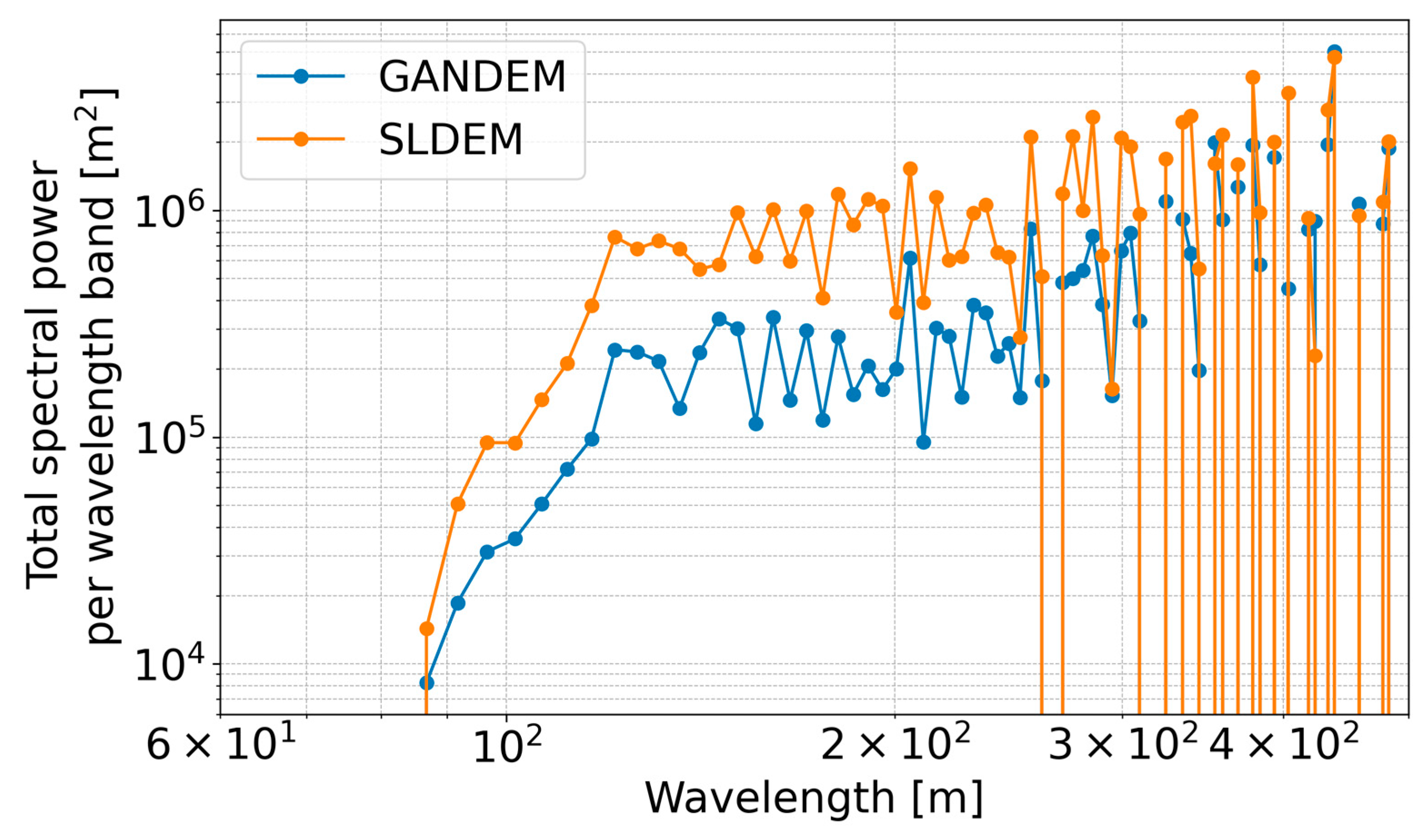
3.1. Generation Result of a High-Resolution DEM

To generate a high-precision DEM of the analyzed region, we trained and developed a GAN model using NACDEMs available in Mare Tranquillitatis, along with the corresponding SLDEMs and LRONAC images for the same locations. The NACDEMs used are for the area surrounding the Apollo 11 landing site and the Mare Tranquillitatis pit site, as shown in Table 1. The Mare Tranquillitatis pit is located at 8.3355°N, 33.222°E [41], and its appearance is shown in Figure S4. The LRONAC images used for training were selected to include a wide range of solar altitude angles. Details are shown in Table 2 and Table 3.
Figure 5 shows SLDEM, NACDEM, and GANDEM for a part of the analyzed region. The NACDEM and GADEM were downsampled to 60 m/pixel. SLDEM contains linear features and localized elevation variations that do not exist in NACDEM. Such artifacts are suppressed in the GANDEM. To assess the improvement in GANDEM quantitatively, we calculated the mean absolute error (MAE), root mean square error (RMSE), and maximum error between NACDEM and SLDEM, as well as between NACDEM and GANDEM (Table 4 and Table 5). In both the Apollo 11 landing site and the Tranquillitatis pit site, the three statistical measures are smaller for the GANDEM results than for the SLDEM results, indicating that GANDEM achieves better reconstruction accuracy. In addition, the MAE and RMSE of the Apollo 11 landing site calculated in an earlier study were 2.76 and 3.02, respectively [25]. Results of this study demonstrate that GANDEM was generated with accuracy comparable to that of the earlier study. Also, GANDEM reconstruction results are almost unchanged when using solar altitude angles ranging from 20° to 70°, as noted in Liu et al. (2022) (see [25] and Supplementary Materials, Text S4).

3.2. Determination of Roughness Parameters at Scales Smaller than the DEM Resolution

In this section, we determined roughness parameters, RMS height ( σ R M S ) and correlation length ( l ), at scales smaller than the DEM resolution. First, we extracted the LRS-received waveforms (A-scan) at each observation point and averaged them. Next, we performed surface scattering simulations in which σ R M S was varied from 1 to 3 m in 1 m intervals, and the correlation length was varied from 10 to 60 m in 10 m intervals. We then created average A-scans using simulation results in the same manner as that used for the observation data. Finally, we adopted the parameters that minimized the sum of absolute differences between the average A-scans of observation and simulation at apparent depths greater than 2 km. This depth threshold was chosen to exclude subsurface echo effects and to examine only scattering from off-nadir surface features. Because earlier studies have detected layered subsurface reflectors in LRS data up to a depth of 2 km in mare regions [4,5,6,7], subsurface echoes might occur up to this depth.
Each panel in Figure 6 shows the averaged observation A-scan (blue lines) and the average simulation A-scan (orange lines) for each parameter condition, with the vertical axis representing the radar power and the horizontal axis representing the apparent depth. The top right of each panel shows the sum of absolute differences between the averaged observation A-scan and simulation A-scan at apparent depths greater than 2 km. The parameters that yield the smallest value of this sum, RMS height σ R M S = 2.0 m and correlation length l = 60 m, are used for the subsequent surface scattering simulations. The results in Figure 6 were obtained using the LRS data, “LRS_SW_WF_05N_032835E.tbl”, and the corresponding simulation results, where the averaged observation A-scans and simulation A-scans were calculated from the average of A-scans for latitudes of 9.55° to 9.8°N.

3.3. Results of Surface Scattering Simulations Using GANDEM

Using the GANDEM generated in Section 3.1 and the roughness parameters determined in Section 3.2, we performed surface scattering simulations for each ground track corresponding to the 15 LRS datasets (Table 6) included in the analyzed region. Figure 7 presents three panels: (a–c), each depicting the LRS observation B-scan, the simulation B-scan using SLDEM, and the simulation B-scan using GANDEM for the ground track of No. 10, displaying latitudes from 9.1° to 9.6°. The simulation results obtained using SLDEM (Figure 7b) show reflection echoes with relatively strong intensity indicated by white circles, which do not appear in the LRS observation data (Figure 7a). By contrast, the simulation results obtained using GANDEM (Figure 7c) show that such artifact echoes are reduced, resulting in a B-scan that is close to the LRS observation B-scan. In Figure 8, histograms show intensity differences between averaged B-scans applied to the processing described in Step 2 of Section 4.2 to the B-scans in Figure 7. The distribution of the intensity difference between the LRS observation data and the SLDEM simulation (shown in blue) has a mean of −0.54 and a standard deviation of 4.9. The negative mean indicates that the SLDEM simulation contains reflection echoes that are not present in the observational data. The distribution of the intensity difference between the LRS observation data and the GANDEM simulation (shown in orange) has a mean of 1.7 and a standard deviation of 4.3. While the positive mean is influenced by a distribution with a peak around 5 dB, the highest probability density is located near 0 dB. Moreover, the standard deviation of the GANDEM case is smaller than that of the SLDEM case, suggesting a reduction in variability in the intensity difference. Furthermore, Figure 9 presents histograms of the reflection intensity differences between the 15 LRS datasets analyzed in this study and their corresponding SLDEM and GANDEM simulations. The histograms only include reflection intensity differences computed at pixel locations where the SLDEM simulation result exhibited strong echo intensities exceeding –25 dB. Similar to the trend observed in Figure 8, the distribution of differences between the LRS observations and the SLDEM simulations shows a negative mean value, indicating the presence of artifact echoes in SLDEM simulations. The distribution of differences between the LRS observations and the GANDEM simulations shows that the highest probability density is located near 0 dB. These results suggest that the GANDEM simulation reduces artifact echoes observed in the SLDEM simulation and enables more accurate surface scattering simulations.

3.4. Detection Results of Subsurface Echoes from LRS Data

We detect subsurface echoes using the method described in Section 2.4. Figure 10 shows the process of calculating the difference between the observation B-scan of No. 4 in Table 6 and the corresponding simulation B-scan. Averaged B-scans (Figure 10c,d) are created from the observation B-scan (Figure 10a) and the simulation B-scan (Figure 10b). The difference is calculated following Step IV in Section 2.4 (Figure 10e). The same processes are applied to the remaining 14 LRS ground tracks. Figure 11 shows the histogram obtained by integrating the difference values from the 15 ground tracks. Using the Gaussian mixture model (GMM), we separated a normal distribution with a mean of 0.630 and a standard deviation of 1.29 and a normal distribution with a mean of 5.18 and a standard deviation of 1.82. The 3 σ 1 line of the normal distribution with a mean closer to 0, namely 4.50, was set as the subsurface echo detection threshold (Supplementary Materials Text S5). The entire process, from performing a surface scattering simulation to determining the subsurface echo detection threshold, was repeated 10 times with different random phases. The statistical measures and thresholds determined for each case are presented in Table 7. Finally, only the pixels that exceeded their respective thresholds in all simulation cases were extracted as SECs.
Figure 12 shows the distribution of the extracted SECs on the SELENE/TC image. Each dot represents an SEC. Its color represents the apparent depth. The three dotted lines represent grabens, which are linear depression structures on the surface. The notable relation is that SECs exist continuously on the northwest extension of graben A, shown by the white solid ellipse. There are no continuous SECs on multiple LRS ground tracks along the extension of grabens A and C. In areas that were not extensional regions of the graben, some SECs were detected continually along multiple LRS ground tracks shown as white dotted ellipses. The SECs have apparent depths of 350–800 m.

3.5. Estimation of Subsurface Structure Indicated by SEC Using the Radar Equation

We investigate whether the intensities of SECs indicate the existence of voids formed at dike tips. The dielectric constant and the attenuation rate of the material above the dike tips are estimated using Equations (12)–(18) with TiO2 and FeO contents and porosity. Using SELENE-Multiband Imager (MI) data [42], we ascertained the average TiO2 and FeO contents in the region along the extension of Graben A, respectively, as 8.5 wt.% and 17.7 wt.%. We adopt a porosity of 10% based on typical basalt porosity from six Apollo rock samples and seven lunar meteorites [43]. Using these values, the true density ( ρ 0 ), the material density assumed porosity ( ρ ), the dielectric constant ( ε 2 ) and the attenuation rate ( γ ) are calculated, respectively, as 3357 kg/m3, 3021 kg/m3, 7.167, and 3.288 × 10⁻² dB/m. The apparent depths of the SECs are approximately 350–800 m. Consequently, the actual depths of the SECs are nearly 130–300 m for the dielectric constant of 7.2. Figure 13 shows an echo intensity plot of dike widths vs. the dielectric constants of the dike tip estimated as described in Section 2.4. Colors represent the intensities of reflected echoes from the boundary between the dike tips and the overlying subsurface material. Echo intensities greater than −25 dB set in Step III of Section 2.3 are observed in cases of dike-tip dielectric constants with 1–4 and dike widths of 50–600 m.

4. Discussion

4.1. Factors Improving Surface Scattering Simulation

In Section 3.3, simulations using GANDEM reduced the artifact echoes seen in simulations using SLDEM and improved consistency with the observation B-scan. To explore the factors underlying this improvement, we performed Fourier transforms for SLDEM and GANDEM, shown in Figure 14. Figure 15 shows a plot of the wavelength of roughness calculated from the spatial frequency obtained by Fourier transform on the horizontal axis and the total spectral power per wavelength band on the vertical axis, with the blue line representing GANDEM and the orange line representing SLDEM. The spectral power is calculated as the squared absolute value of the Fourier-transformed amplitude. This represents the elevation variance at each wavelength (i.e., the intensity of topographic undulation). The figure shows that the total spectral power of SLDEM is several times higher than that of GANDEM in the wavelength range of 80–300 m. The increase in the total spectral power of SLDEM in this wavelength range corresponds to the linear artifacts or localized rise features indicated by the white circle and white arrows in Figure 14a. SLDEM2015 was generated by co-registering the DEM (SLDEM2013), derived from the SELENE/Terrain Camera (TC) images, with the terrain elevations measured by the Lunar Orbiter Laser Altimeter (LOLA) on each 1° × 1° tile [20]. This tile-based approach results in linear discontinuities between adjacent tiles. The localized rise features may be attributed to reduced DEM accuracy caused by limitations in the TC camera resolution, attitude reconstruction errors, and orbit determination errors. The increase in such short-wavelength artifact roughness, which is close to the LRS central wavelength (60 m), is thought to scatter the LRS signal more than in reality, resulting in the artifact echoes on the simulation B-scan.
Next, we demonstrate whether roughness with a wavelength of 80–300 m can occur in the artifact echoes in a simulation B-scan. Figure 16 shows the elevation map of the SLDEM and the B-scans where artifact echoes were observed in Figure 7b. Figure 16a,b shows the original SLDEM and the corresponding simulation result, respectively. Figure 16c,e presents the elevation maps in which a 300 m Gaussian filter has been applied to part of the region, and Figure 16d,f shows the simulation results using those filtered DEMs. When localized rise features highlighted by the white circle in Figure 16a are smoothed by the Gaussian filter, the artifact echoes seen in Figure 16b are reduced, as shown in Figure 16d,f. These results suggest that localized rise features in SLDEM can generate artifact echoes in surface scattering simulations.
Finally, we investigate the effectiveness of GANDEM in reducing short-wavelength artifact roughness present in SLDEM. We applied a Gaussian filter with a 300 m kernel size to GANDEM, SLDEM, and NACDEM, acquiring the low-frequency topography. And we extracted the high-frequency components by subtracting the filtered DEMs from the original DEMs. Table 8 and Table 9 summarize the MAE and RMSE values comparing the low- and high-frequency components of SLDEM and GANDEM with those of NACDEM. The MAE and RMSE of the low-frequency components are comparable between the NACDEM–SLDEM case and the NACDEM–GANDEM case, indicating that the improvement in GANDEM on large-scale topographic structures (>300 m) is limited. In contrast, the MAE and RMSE of the high-frequency components are clearly lower for GANDEM. These results suggest that GANDEM effectively improves small-scale topographic structures (<300 m) resulting in the artifact echoes on the simulation B-scan.

4.2. Detection Validity of Subsurface Echo Candidates

In earlier comparative analyses using radar observation data and surface scattering simulation, no attempts have been made to extract small-scale subsurface echoes in the horizontal direction by subtracting simulation data from observation data. This absence of such an earlier study has occurred because meaningful subsurface echoes have not been identifiable, caused by echo position and reflection intensity errors. These errors result from low accuracy of DEM data, failure to consider small-scale roughness that cannot be expressed by DEM, and LRS position uncertainty. For this study, we have generated a GANDEM that improves upon SLDEM. Additionally, to compensate for echo shifts caused by DEM inaccuracies and LRS positioning errors, we calculated the intensity difference not only with single pixels but also with the surrounding pixels. Furthermore, by averaging the original B-scan to 600 m/pixel horizontally, this detection method satisfies the subsurface echo detection criteria for LRS outlined by [18], which require continuous detection over 600 m in the horizontal direction. Since the apparent depths of the SECs (350–800 m) are relatively shallow, SECs could be caused by side lobes of the LRS signal. An ideal reflection pattern resulting from the LRS transmitted signal reflecting off a perfectly flat lunar surface is provided in the Supplementary Figure S7. The reflection intensity at the apparent depth of the SECs (350–800 m) is reduced to approximately –40 to –60 dB, which is sufficiently less than the reflection intensity of SECs (–25 dB). Therefore, it is unlikely that the sidelobes cause SECs (Supplementary Materials Text S6).
This method has several limitations. First, it is not possible to ascertain whether a subsurface echo exists in an area where a strong reflected echo exists in both the observation B-scan and the simulation B-scan. This method can only investigate whether subsurface echoes exist in an area where there is no strong echo caused by surface scattering. A second limitation is the range of applicability of roughness parameters below the resolution of DEM. An analysis for determining the roughness parameters (Section 3.2) was performed for one set of LRS data within the analyzed region. Then the determined parameters were used for all the simulations. However, the characteristics of small-scale roughness might vary in different lunar mare regions or in units with different surface compositions or ages even within the same mare region. If the roughness parameters are not set correctly for each region, the simulation will not be able to simulate surface scattering echoes accurately. Consequently, false detections or missed detections of SEC are likely to occur frequently. Future application of this method to the entire Moon will require determination of the roughness parameters for each region.

4.3. Subsurface Structures Indicated by SECs

SECs have been observed along the northwestward extension of graben A. Grabens are often formed by subsurface magma intrusions [39]. The SECs found in the extension of Graben A probably reflect the subsurface structure caused by the subsurface magma intrusion that formed Graben A. Furthermore, SECs have been detected continuously on LRS multiple ground tracks, even in areas that are not extensions of a graben. Those results are thought to indicate a subsurface structure caused by subsurface magma intrusion or other subsurface structure that continues in the horizontal direction.
Radar equation analysis, assuming that SECs are related to subsurface magma intrusion, can explain the intensities of SECs (stronger than −25 dB) when a dike is 50–600 m wide and when the dielectric constant of a dike tip is between 1 and 4. The dielectric constant of 1 represents a void. A dielectric constant of 2–4 corresponds to a porosity of approximately 35–70% for the dike-tip material, assuming that the magma within the dike has the same true density (3357 kg/m3) as the surrounding rock. Therefore, SECs can indicate voids or fillings of high-porosity material shallow subsurface (hereinafter, these two are designated collectively as “void structures”).
Next, we discuss whether other subsurface structures can explain the intensities and distributions of SECs. The echo intensities reflected from regolith layers between lava layers have already been detected in previous LRS studies and can exceed −25 dB [4]. However, such regolith layers should be formed horizontally over hundreds of square kilometers. The SECs detected along the extension of the graben or continuously on multiple LRS ground tracks are unlikely to be reflected echoes from the regolith layers. A fault might be the subsurface structures returning the echo intensities exceeding −25 dB. A fault plane could be a strong reflection source if it were to lie perpendicularly to the radar emission vector. Because the lunar fault angle has been estimated as an average of 60° [44], strong reflections would be returned only from faults approximately 200 km distant from the spacecraft at 100 km altitude. In such a case, SECs can be expected to be detected at the apparent depth of 200 km, much deeper than the 350–800 m apparent depths from the LRS data. Consequently, no fault could be the reflection source for the SECs. Layers of ice and liquid water returning strong radar echoes have been discovered under the surface of Mars [3], but those would not exist in the lunar equatorial region. Next, we consider fracture zones that may have been locally formed by meteoroid impacts and lunar crustal deformation. The results shown in Figure 13 suggest that if the porosity of fracture zones exceeds 35% (corresponding to a dielectric constant below 4), reflected waves from fracture zones can cause SECs. Although the average porosity of the upper lunar crust has been estimated to be 12% based on GRAIL data [36], it remains unclear whether local fracture zones can exceed 35% porosity. To determine whether the SECs indicate subsurface localized fracture zones, it is necessary to evaluate the spatial distribution of SECs over a large area and assess their correlation with surface features indicative of tectonic deformation.
Possible subsurface void structures along multiple LRS ground tracks are considered to be lava tubes [14,45] and gas voids at magma tips [11]. Lava tubes tend to be oriented in a downward elevation direction. Figure 17 shows the SLDEM2015 elevation data for the analyzed region, with overlaid contour lines. As shown in this figure, the SECs detected across multiple LRS ground tracks, identified by the dotted ellipse in Figure 12, are more or less aligned in the downward elevation direction, suggesting the possible presence of lava tubes. By contrast, the SECs along the extension of Graben A (Figure 12) are distributed parallel to the contour lines. Considering that the SECs are located along the extension of the graben, the most plausible explanation is that they represent gas voids at the tips of the intrusive magma that formed the graben.

5. Conclusions

We propose a method for detecting small-scale subsurface echoes, of approximately the LRS azimuth resolution (hundreds of meters), from Lunar Radar Sounder (LRS) data. To evaluate surface scattering effects accurately, we perform surface scattering simulations using a high-resolution DEM generated with a GAN (GANDEM), which provides greater accuracy than when using SLDEM. In this simulation, we also calculate incoherent scattering, assuming random roughness smaller than the DEM resolution. After the LRS B-scan and simulation B-scan are downsampled to the LRS resolution range, a detection threshold for subsurface echoes is determined from the histogram of their differences, enabling the extraction of SECs.
The simulation using GANDEM showed that the artifact echoes seen in the results obtained using SLDEM were suppressed. Agreement with the LRS observation B-scan was improved because the linear and localized low-frequency artifact topographies included in the SLDEM were suppressed by GANDEM. Some SECs were present in the extension area of the graben. Also, SECs were found continuously across multiple LRS ground tracks in areas not related to grabens. We examined whether the echo intensities of SECs (>−25 dB) might result from reflections off subsurface voids and found that this intensity is accounted for when the void width is 50–600 m and the subsurface structure’s dielectric constant is 1–4. This dielectric constant indicated that the subsurface structure was a void or a material with high porosity. These results suggest that the SECs present in the extension area of the graben and the SECs detected continuously on multiple LRS ground tracks are likely to be from subsurface void structures that exist continuously in the horizontal direction, such as gas voids at the magma tip or lava tubes.
This method can be a powerful tool to detect lava tubes and subsurface gas voids predicted by earlier studies. It can contribute to the selection of future manned bases and can lead to further constraints on lunar magmatic volatiles. Furthermore, the lunar surface roughness parameterization analysis performed using this method can elucidate small-scale roughness that cannot be evaluated by DEM from radar data. It can contribute to understanding the lunar surface characteristics and to facilitating landing site selection.

Supplementary Materials

The following supporting information can be downloaded at: https://www.mdpi.com/article/10.3390/rs17101710/s1. References [45,46,47,48] are cited in the Supplementary Materials file.

Author Contributions

Conceptualization, H.N. and J.H.; methodology, H.N., J.H., A.K. and R.O.; software, H.N. and A.K.; validation, H.N., J.H., A.K., T.I., K.T. and R.O.; formal analysis, H.N.; investigation, H.N.; resources, A.K. and J.W.H.; writing—original draft preparation, H.N. and J.W.H.; writing—review and editing, H.N., J.H., A.K., T.I., K.T., J.W.H. and R.O.; visualization, H.N.; project administration, H.N., J.H., T.I. and R.O.; funding acquisition, H.N., J.H. and T.I. All authors have read and agreed to the published version of the manuscript.

Funding

This work was supported by JST SPRING (grant numbers JPMJSP2104).

Data Availability Statement

The LRONAC images are available at https://ode.rsl.wustl.edu/moon/index.aspx (accessed on 1 September 2024). NACDEM data can be downloaded from https://pds.lroc.asu.edu/data/LRO-L-LROC-5-RDR-V1.0/LROLRC_2001/DATA/SDP/NAC_DTM/ (accessed on 1 September 2024). SELENE/LRS data are available at https://data.darts.isas.jaxa.jp/pub/pds3/sln-l-lrs-2-sndr-waveform-high-v1.0/ (accessed on 10 April 2022). SELENE/MI data used to estimate FeO and TiO2 contents on the lunar surface can be obtained at https://data.darts.isas.jaxa.jp/pub/pds3/sln-l-mi-5-map-v3.0/ (accessed on 10 April 2022). TC image data are available at https://data.darts.isas.jaxa.jp/pub/pds3/sln-l-tc-5-ortho-map-v2.0/ (accessed on 10 April 2022). GRAIL crust thickness data can be accessed at https://zenodo.org/records/997347 (accessed on 10 April 2022). Thorium content data obtained from gamma-ray data of Lunar Prospector are available at https://pds-geosciences.wustl.edu/missions/lunarp/reduced_special.html (accessed on 10 April 2022). SLDEM2015 http://imbrium.mit.edu/DATA/SLDEM2015/ (accessed on 10 April 2022). Anyone can download these data for free.

Acknowledgments

We thank the JAXA team that built and operated the spacecraft SELENE/Kaguya and led this mission to success. We are grateful the LRS team for creating datasets and documenting how they are handled. We thank N. Geshi for his comments, which led to considerable improvement of the discussion section.

Conflicts of Interest

The authors declare no conflicts of interest.

References

  1. Plaut, J.J.; Picardi, G.; Safaeinili, A.; Ivanov, A.B.; Milkovich, S.M.; Cicchetti, A.; Kofman, W.; Mouginot, J.; Farrell, W.M.; Phillips, R.J.; et al. Subsurface Radar Sounding of the South Polar Layered Deposits of Mars. Science 2007, 316, 92–95. [Google Scholar] [CrossRef]
  2. Holt, J.W.; Safaeinili, A.; Plaut, J.J.; Head, J.W.; Phillips, R.J.; Seu, R.; Kempf, S.D.; Choudhary, P.; Young, D.A.; Putzig, N.E.; et al. Radar Sounding Evidence for Buried Glaciers in the Southern Mid-Latitudes of Mars. Science 2008, 322, 1235–1238. [Google Scholar] [CrossRef] [PubMed]
  3. Orosei, R.; Lauro, S.E.; Pettinelli, E.; Cicchetti, A.; Coradini, M.; Cosciotti, B.; Di Paolo, F.; Flamini, E.; Mattei, E.; Pajola, M.; et al. Radar Evidence of Subglacial Liquid Water on Mars. Science 2018, 361, 490–493. [Google Scholar] [CrossRef]
  4. Ono, T.; Kumamoto, A.; Nakagawa, H.; Yamaguchi, Y.; Oshigami, S.; Yamaji, A.; Kobayashi, T.; Kasahara, Y.; Oya, H. Lunar Radar Sounder Observations of Subsurface Layers under the Nearside Maria of the Moon. Science 2009, 323, 909–912. [Google Scholar] [CrossRef] [PubMed]
  5. Oshigami, S.; Okuno, S.; Yamaguchi, Y.; Ohtake, M.; Haruyama, J.; Kobayashi, T.; Kumamoto, A.; Ono, T. The Layered Structure of Lunar Maria: Identification of the HF-Radar Reflector in Mare Serenitatis Using Multiband Optical Images. Icarus 2012, 218, 506–512. [Google Scholar] [CrossRef]
  6. Oshigami, S.; Watanabe, S.; Yamaguchi, Y.; Yamaji, A.; Kobayashi, T.; Kumamoto, A.; Ishiyama, K.; Ono, T. Mare Volcanism: Reinterpretation Based on Kaguya Lunar Radar Sounder Data. J. Geophys. Res. Planets 2014, 119, 1037–1045. [Google Scholar] [CrossRef]
  7. Ishiyama, K.; Kumamoto, A. Volcanic History in the Smythii Basin Based on SELENE Radar Observation. Sci. Rep. 2019, 9, 14502. [Google Scholar] [CrossRef] [PubMed]
  8. Ishiyama, K.; Kumamoto, A.; Ono, T.; Yamaguchi, Y.; Haruyama, J.; Ohtake, M.; Katoh, Y.; Terada, N.; Oshigami, S. Estimation of the Permittivity and Porosity of the Lunar Uppermost Basalt Layer Based on Observations of Impact Craters by SELENE. J. Geophys. Res. Planets 2013, 118, 1453–1467. [Google Scholar] [CrossRef]
  9. Hongo, K.; Toh, H.; Kumamoto, A. Estimation of Bulk Permittivity of the Moon’s Surface Using Lunar Radar Sounder on-Board Selenological and Engineering Explorer. Earth Planets Space 2020, 72, 1–15. [Google Scholar] [CrossRef]
  10. Kobayashi, T.; Kim, J.H.; Lee, S.R.; Araki, H.; Ono, T. Simultaneous Observation of Lunar Radar Sounder and Laser Altimeter of Kaguya for Lunar Regolith Layer Thickness Estimate. IEEE Geosci. Remote Sens. Lett. 2010, 7, 435–439. [Google Scholar] [CrossRef]
  11. Head, J.W.; Wilson, L. Generation, Ascent and Eruption of Magma on the Moon: New Insights into Source Depths, Magma Supply, Intrusions and Effusive/Explosive Eruptions (Part 2: Predicted Emplacement Processes and Observations). Icarus 2017, 283, 176–223. [Google Scholar] [CrossRef]
  12. Wilson, L.; Head, J.W. Eruption of Magmatic Foams on the Moon: Formation in the Waning Stages of Dike Emplacement Events as an Explanation of “Irregular Mare Patches”. J. Volcanol. Geotherm. Res. 2017, 335, 113–127. [Google Scholar] [CrossRef]
  13. Head, J.W.; Ivanov, B. Impact Cratering at the Lunar Ina Irregular Mare Patch (IMP): Experimental Evidence for the Nature of Impacts into Porous Basaltic Substrate and Outstanding Questions. Planet. Space Sci. 2024, 250, 105954. [Google Scholar] [CrossRef]
  14. Haruyama, J.; Hioki, K.; Shirao, M.; Morota, T.; Hiesinger, H.; van der Bogert, C.H.; Miyamoto, H.; Iwasaki, A.; Yokota, Y.; Ohtake, M.; et al. Possible Lunar Lava Tube Skylight Observed by SELENE Cameras. Geophys. Res. Lett. 2009, 36, L21206. [Google Scholar] [CrossRef]
  15. Kaku, T.; Haruyama, J.; Miyake, W.; Kumamoto, A.; Ishiyama, K.; Nishibori, T.; Yamamoto, K.; Crites, S.T.; Michikami, T.; Yokota, Y.; et al. Detection of Intact Lava Tubes at Marius Hills on the Moon by SELENE (Kaguya) Lunar Radar Sounder. Geophys. Res. Lett. 2017, 44, 10–155. [Google Scholar] [CrossRef]
  16. Chappaz, L.; Sood, R.; Melosh, H.J.; Howell, K.C.; Blair, D.M.; Milbury, C.; Zuber, M.T. Evidence of Large Empty Lava Tubes on the Moon Using GRAIL Gravity. Geophys. Res. Lett. 2017, 44, 105–112. [Google Scholar] [CrossRef]
  17. Zhu, K.; Yang, M.; Yan, X.Y.; Li, W.K.; Feng, W.; Zhong, M. GRAIL Gravity Gradients Evidence for a Potential Lava Tube at Marius Hills on the Moon. Icarus 2024, 408, 115814. [Google Scholar] [CrossRef]
  18. Kobayashi, T.; Kim, J.-H.; Lee, S.R.; Song, K.-Y. Nadir Detection of Lunar Lava Tube by Kaguya Lunar Radar Sounder. IEEE Trans. Geosci. Remote Sens. 2020, 59, 7395–7418. [Google Scholar] [CrossRef]
  19. Donini, E.; Carrer, L.; Gerekos, C.; Bruzzone, L.; Bovolo, F. An Unsupervised Fuzzy System for the Automatic Detection of Candidate Lava Tubes in Radar Sounder Data. Geosci. Remote Sens. 2022, 60, 1–19. [Google Scholar] [CrossRef]
  20. Barker, M.K.; Mazarico, E.; Neumann, G.A.; Zuber, M.T.; Haruyama, J.; Smith, D.E. A New Lunar Digital Elevation Model from the Lunar Orbiter Laser Altimeter and SELENE Terrain Camera. Icarus 2016, 273, 346–355. [Google Scholar] [CrossRef]
  21. Wu, B.; Liu, W.C.; Grumpe, A.; Wöhler, C. Construction of Pixel-Level Resolution DEMs from Monocular Images by Shape and Albedo from Shading Constrained with Low-Resolution DEM. ISPRS J. Photogramm. Remote Sens. 2018, 140, 3–19. [Google Scholar] [CrossRef]
  22. Tao, Y.; Muller, J.P.; Conway, S.J.; Xiong, S. Large Area High-Resolution 3d Mapping of Oxia Planum: The Landing Site for the Exomars Rosalind Franklin Rover. Remote Sens. 2021, 13, 3270. [Google Scholar] [CrossRef]
  23. Chen, L.-C.; Papandreou, G.; Kokkinos, I.; Murphy, K.; Yuille, A.L. DeepLab: Semantic Image Segmentation with Deep Convolutional Nets, Atrous Convolution, and Fully Connected CRFs. IEEE Trans. Pattern Anal. Mach. Intell. 2017, 40, 834–848. [Google Scholar] [CrossRef] [PubMed]
  24. Chen, H.; Hu, X.; Oberst, J. Pixel-Resolution Dtm Generation for the Lunar Surface Based on a Combined Deep Learning and Shape-from-Shading (Sfs) Approach. ISPRS Ann. Photogramm. Remote Sens. Spat. Inf. Sci. 2022, 3, 511–516. [Google Scholar] [CrossRef]
  25. Liu, Y.; Wang, Y.; Di, K.; Peng, M.; Wan, W.; Liu, Z. A Generative Adversarial Network for Pixel-Scale Lunar DEM Generation from High-Resolution Monocular Imagery and Low-Resolution DEM. Remote Sens. 2022, 14, 5420. [Google Scholar] [CrossRef]
  26. Gerekos, C.; Haynes, M.S.; Schroeder, D.M.; Blankenship, D.D. The Phase Response of a Rough Rectangular Facet for Radar Sounder Simulations of Both Coherent and Incoherent Scattering. Radio Sci. 2023, 58, 1–30. [Google Scholar] [CrossRef]
  27. Berquin, Y.; Herique, A.; Kofman, W.; Heggy, E. Computing Low-Frequency Radar Surface Echoes for Planetary Radar Using Huygens-Fresnel’s Principle. Radio. Sci. 2015, 50, 1097–1109. [Google Scholar] [CrossRef]
  28. Ono, T.; Kumamoto, A.; Kasahara, Y.; Yamaguchi, Y.; Yamaji, A.; Kobayashi, T.; Oshigami, S.; Nakagawa, H.; Goto, Y.; Hashimoto, K.; et al. The Lunar Radar Sounder (LRS) Onboard TheáKAGUYA (SELENE) Spacecraft. Space Sci. Rev. 2010, 154, 145–192. [Google Scholar] [CrossRef]
  29. Kobayashi, T.; Kim, J.H.; Lee, S.R.; Kumamoto, A.; Nakagawa, H.; Oshigami, S.; Oya, H.; Yamaguchi, Y.; Yamaji, A.; Ono, T. Synthetic Aperture Radar Processing of Kaguya Lunar Radar Sounder Data for Lunar Subsurface Imaging. IEEE Trans. Geosci. Remote Sens. 2012, 50, 2161–2174. [Google Scholar] [CrossRef]
  30. Bishop, C.M.; Nasrabadi, N.M. Pattern Recognition and Machine Learning; Springer: New York, NY, USA, 2006. [Google Scholar]
  31. Goossens, S.; Matsumoto, K.; Rowlands, D.D.; Lemoine, F.G.; Noda, H.; Araki, H. Orbit Determination of the SELENE Satellites Using Multi-Satellite Data Types and Evaluation of SELENE Gravity Field Models. J. Geod. 2011, 85, 487–504. [Google Scholar] [CrossRef]
  32. Carrier, W.D., III; Olhoeft, G.R.; Mendell, W. Physical properties of the lunar surface. In Lunar Sourcebook, a User’s Guide to the Moon; Cambridge University Press: Cambridge, UK, 1991. [Google Scholar]
  33. Olhoeft, G.R.; Strangway, D.W. Dielectric Properties of the First 100 Meters of the Moon. Earth Planet. Sci. Lett. 1975, 24, 394–404. [Google Scholar] [CrossRef]
  34. Chyba, C.F.; Ostro, S.J.; Edwards, B.C. Radar Detectability of a Subsurface Ocean on Europa. Icarus 1998, 134, 292–302. [Google Scholar] [CrossRef]
  35. Ishihara, Y.; Goossens, S.; Matsumoto, K.; Noda, H.; Araki, H.; Namiki, N.; Hanada, H.; Iwata, T.; Tazawa, S.; Sasaki, S. Crustal Thickness of the Moon: Implications for Farside Basin Structures. Geophys. Res. Lett. 2009, 36, L19202. [Google Scholar] [CrossRef]
  36. Wieczorek, M.A.; Neumann, G.A.; Nimmo, F.; Kiefer, W.S.; Taylor, G.J.; Melosh, H.J.; Phillips, R.J.; Solomon, S.C.; Andrews-Hanna, J.C.; Asmar, S.W.; et al. The Crust of the Moon as Seen by GRAIL. Science 2013, 339, 671–675. [Google Scholar] [CrossRef]
  37. Kobayashi, S.; Karouji, Y.; Morota, T.; Takeda, H.; Hasebe, N.; Hareyama, M.; Kobayashi, M.; Shibamura, E.; Yamashita, N.; d’Uston, C.; et al. Lunar Farside Th Distribution Measured by Kaguya Gamma-Ray Spectrometer. Earth Planet. Sci. Lett. 2012, 337, 10–16. [Google Scholar] [CrossRef]
  38. Lawrence, D.J.; Puetter, R.C.; Elphic, R.C.; Feldman, W.C.; Hagerty, J.J.; Prettyman, T.H.; Spudis, P.D. Global Spatial Deconvolution of Lunar Prospector Th Abundances—Lawrence—2007—Geophysical Resea. Geophys. Res. Lett. 2007, 34, L03201. [Google Scholar] [CrossRef]
  39. Head, J.W.; Wilson, L. Lunar Graben Formation Due to Near-Surface Deformation Accompanying Dike Emplacement Introduction and Background. Planet. Space Sci. 1993, 41, 719–727. [Google Scholar] [CrossRef]
  40. Haruyama, J.; Matsunaga, T.; Ohtake, M.; Morota, T.; Honda, C.; Yokota, Y.; Torii, M.; Ogawa, Y. Global Lunar-Surface Mapping Experiment Using the Lunar Imager/Spectrometer on SELENE. Earth Planets Space 2008, 60, 243–255. [Google Scholar] [CrossRef]
  41. Robinson, M.S.; Ashley, J.W.; Boyd, A.K.; Wagner, R.V.; Speyerer, E.J.; Ray Hawke, B.; Hiesinger, H.; Van Der Bogert, C.H. Confirmation of Sublunarean Voids and Thin Layering in Mare Deposits. Planet. Space Sci. 2012, 69, 18–27. [Google Scholar] [CrossRef]
  42. Otake, H.; Ohtake, M.; Hirata, N. Lunar Iron and Titanium Abundance Algorithms Based on SELENE (Kaguya) Multiband Imager Data. In Proceedings of the 43rd Annual Lunar and Planetary Science Conference, Woodlands, TX, USA, 19–23 March 2012; p. 1905. [Google Scholar]
  43. Kiefer, W.S.; MacKe, R.J.; Britt, D.T.; Irving, A.J.; Consolmagno, G.J. The Density and Porosity of Lunar Rocks. Geophys. Res. Lett. 2012, 39, L07201. [Google Scholar] [CrossRef]
  44. Golombek, M.P. Structural Analysis of Lunar Grabens and the Shallow Crustal Structure of the Moon. J. Geophys. Res. Solid. Earth 1979, 84, 4657–4666. [Google Scholar] [CrossRef]
  45. Wilson, L.; Head, J.W. Controls on Lunar Basaltic Volcanic Eruption Structure and Morphology: Gas Release Patterns in Sequential Eruption Phases. Geophys. Res. Lett. 2018, 45, 5852–5859. [Google Scholar] [CrossRef]
  46. Wilson, L.; Head, J.W., III. Deep Generation of Magmatic Gas on the Moon and Implications for Pyroclastic Eruptions. Geophys. Res. Lett. 2003, 30, 1605. [Google Scholar] [CrossRef]
  47. Head, J.W.; Wilson, L.; Hiesinger, H.; van der Bogert, C.; Chen, Y.; Dickson, J.L.; Gaddis, L.R.; Haruyama, J.; Jawin, E.R.; Jozwiak, L.M.; et al. Lunar Mare Basaltic Volcanism: Volcanic Features and Emplacement Processes. Rev. Mineral. Geochem. 2023, 89, 453–507. [Google Scholar] [CrossRef]
  48. Rutherford, M.J.; Head, J.W.; Saal, A.E.; Hauri, E.; Wilson, L. Model for the Origin, Ascent, and Eruption of Lunar Picritic Magmas. Am. Mineral. 2017, 102, 2045–2053. [Google Scholar] [CrossRef]
Figure 1. Overall process of subsurface echo detection method from Lunar Radar Sounder (LRS) data.
Remotesensing 17 01710 g001
Figure 2. Schematic diagram of the radar equation analysis for reflection intensity from the subsurface dike tip. A s u r and A s u b , respectively, represent the radar illuminated area of the surface and the subsurface. ε 0 , ε 1 and ε 2 , respectively, stand for the dielectric constants of vacuum, the host basalt, and the dike-tip material.
Remotesensing 17 01710 g002
Figure 5. Comparison of different DEMs: (a) SLDEM2015; (b) NACDEM; (c) GANDEM downsampled with 60 m/pixel; (d) original GANDEM.
Remotesensing 17 01710 g005
Figure 6. (ar) Averaged observation A-scans (blue lines) and averaged simulation A-scans (orange lines) for various RMS heights σ R M S and correlation lengths l . The vertical axis represents radar power, and the horizontal axis represents apparent depth, which assuming a dielectric constant of the subsurface medium is one. The RMS heights σ R M S and correlation lengths l used are shown at the top of each panel. The top right of each panel shows the sum of absolute differences between the averaged observation A-scan and simulation A-scan at apparent depths greater than 2 km.
Remotesensing 17 01710 g006
Figure 7. Effects of using different DEMs on simulated B-scan: (a) LRS observation B-scan; (b) simulation B-scan using SLDEM; (c) simulation B-scan using GANDEM.
Remotesensing 17 01710 g007
Figure 8. Intensity differences between averaged B-scans applied the processing described in Step 2 of Section 4.2 to the B-scans in Figure 7. The blue histogram shows the intensity difference between LRS observation and the simulation using SLDEM. The orange histogram shows the intensity difference between LRS observation and the simulation using GANDEM.
Remotesensing 17 01710 g008
Figure 9. Intensity differences between the 15 LRS datasets analyzed in this study and their corresponding SLDEM and GANDEM simulations. This figure includes reflection intensity differences computed at pixel locations where the reflection intensities in SLDEM simulations exceed –25 dB. The blue histogram shows the intensity difference between LRS observation and the simulation using SLDEM. The orange histogram shows the intensity difference between LRS observation and the simulation using GANDEM.
Remotesensing 17 01710 g009
Figure 10. Flow to detecting subsurface echo signals using observation and simulation B-scans. Panels (a) and (b), respectively, show an LRS observation B-scan and a simulation B-scan. Panels (c) and (d), respectively, show the averaged B-scans of panels (a) and (b). Panel (e) shows the difference calculated following Step IV in Section 2.4.
Remotesensing 17 01710 g010
Figure 11. Histogram of the difference d I for simulation case No. 1. The normal distribution 1 (red) represents the one with a mean value close to zero among the two distributions and corresponds to surface scattering components. The normal distribution 2 (green), with a positive mean value, represents the distribution of subsurface echo candidates. The dashed line indicates the 3 σ value of the normal distribution 1 (i.e. 3.7).
Remotesensing 17 01710 g011
Figure 12. Distribution of the subsurface echo candidates (SECs) on the SELENE/TC image. Each dot represents an SEC. Its color represents the apparent depth, which assuming a dielectric constant of the subsurface medium is one. The three dotted lines represent grabens. The solid white ellipse indicates clusters of SECs aligned along Graben A. The dashed white ellipses highlight areas where SECs are continuously detected along multiple LRS ground tracks, with no corresponding surface topographic features.
Remotesensing 17 01710 g012
Figure 13. Plot of reflected echo intensities as a function of subsurface structure width along the satellite track and dielectric constants of subsurface dike tips calculated using radar equation analysis. The dielectric constant and attenuation rate of the host basalt rock were set, respectively, as 7.2 and 0.032 dB/m.
Remotesensing 17 01710 g013
Figure 14. Comparison of SLDEM (a) and GANDEM (b). The solid white circle in panel (a) indicates linear artifacts along the latitudinal direction. The white arrows show localized rise features. Similar artifacts can also be seen in Figure 5.
Remotesensing 17 01710 g014
Figure 15. Total spectral power per wavelength band of roughness included in SLDEM and GANDEM. Blue and orange lines, respectively, represent the results of GANDEM and SLDEM.
Remotesensing 17 01710 g015
Figure 16. Investigation of terrain that produces artifact echoes in simulation B-scan using SLDEM. (a) Original SLDEM; (b) simulation result using SLDEM shown in (a); (c) DEM with Gaussian filter applied to the area indicated by the white circle; (d) simulation result using SLDEM shown in (c); (e) DEM with Gaussian filter applied to the area indicated by the white circle; (f) simulation result using SLDEM shown in (e).
Remotesensing 17 01710 g016
Figure 17. Surface elevation map produced using SLDEM2015 in the analyzed region. Gray dotted lines are contour lines. White dotted lines show grabens. Solid and dotted ellipses indicate the locations of SECs detected across multiple LRS ground tracks in Figure 12.
Remotesensing 17 01710 g017
Table 1. Details of the NACDEMs used for training.
AreaData NameCenter Position
Latitude (°N), Longitude (°E)
Apollo 11NAC_DTM_APOLLO11_E008N0234.IMG0.77, 23.44
Tranquillitatis pitNAC_DTM_TRANQPIT1_E084N0332.IMG8.39, 33.19
Table 2. Solar altitude angles of the LRO images used for training at the Apollo 11 landing site.
IDData NameSolar Altitude Angle (°)
(LE, RE)
IDData NameSolar Altitude Angle (°)
(LE, RE)
1M111165641418.35, 18.27M119766100558.69, 57.98
2M15036181727.46, 27.398M130229196759.44, 59.29
3M10436219936.22, 36.039M10671977462.77, 62.57
4M115995634443.17, 43.0110M18807123172.51, 72.29
5M112107452749.08, 48.9111M111637978773.36, 73.17
6M112108872651.02, 50.8512M18809982276.22, 75.99
Table 3. Solar altitude angles of the LRO images used for training at the Tranquillitatis pit site.
IDData NameSolar Altitude Angle (°)
(LE, RE)
IDData NameSolar Altitude Angle (°)
(LE, RE)
1M123050501222.67, 22.548M145834640350.49, 50.29
2M131985566928.79, 28.669M15265523754.2, 54.13
3M127989211132.09, 31.9410M147823946356.00, 55.77
4M142198011938.65, 38.4211M128694729363.81, 63.68
5M122111571743.88, 43.5312M144544898469.59, 69.47
6M111395063845.38, 45.2213M122345780670.89, 70.72
7M19038027147.56, 47.3814M18802135173.46, 73.3
Table 4. Error statistics between SLDEM and NACDEM in the two areas.
RegionMAE (m)RMSE (m)Maximum Error (m)
Apollo 112.363.1627.0
Tranquillitatis pit2.934.0929.4
Table 5. Error statistics between GANDEM and NACDEM in the two areas.
RegionMAE (m)RMSE (m)Maximum Error (m)
Apollo 112.042.6417.6
Tranquillitatis pit2.253.3123.7
Table 6. List of LRS datasets used for this study.
No.Data NameNo.Data Name
1LRS_SW_WF_05N_032145E.tbl9LRS_SW_WF_05N_033232E.tbl
2LRS_SW_WF_05N_032278E.tbl10LRS_SW_WF_05N_033344E.tbl
3LRS_SW_WF_05N_032336E.tbl11LRS_SW_WF_05N_033405E.tbl
4LRS_SW_WF_05N_032444E.tbl12LRS_SW_WF_05N_033510E.tbl
5LRS_SW_WF_05N_032617E.tbl13LRS_SW_WF_05N_033686E.tbl
6LRS_SW_WF_05N_032804E.tbl14LRS_SW_WF_05N_033873E.tbl
7LRS_SW_WF_05N_032835E.tbl15LRS_SW_WF_05N_033905E.tbl
8LRS_SW_WF_05N_033101E.tbl
Table 7. Statistical measures of the distribution of surface scattering and the subsurface echo detection threshold obtained in each simulation case.
Simulation No.Normal Distribution 1
(Mean, Standard Derivation)
Normal Distribution 2
(Mean, Standard Derivation)
Threshold
10.449, 1.094.39, 1.493.70
20.439, 1.014.33, 1.673.46
30.474, 1.124.67, 1.563.84
40.478, 1.034.44, 1.643.56
50.373, 1.024.54, 1.593.44
60.431, 1.024.22, 1.503.49
70.516, 1.094.61, 1.583.78
80.482, 1.094.50, 1.493.76
90.357, 1.074.28, 1.563.43
100.476, 1.074.37, 1.533.67
Table 8. MAE between NACDEM–SLDEM and NACDEM–GANDEM in the two areas.
NACDEM–SLDEM
MAE (m)
NACDEM–GANDEM
MAE (m)
Apollo 11 site
Low-frequency topography
1.431.41
Apollo 11 site
High-frequency topography
2.001.34
Tranquillitatis pit site
Low-frequency topography
1.641.49
Tranquillitatis pit site
High-frequency topography
2.471.77
Table 9. RMSE between NACDEM–SLDEM and NACDEM–GANDEM in the two areas.
NACDEM–SLDEM
RMSE (m)
NACDEM–GANDEM
RMSE (m)
Apollo 11 site
Low-frequency topography
1.741.72
Apollo 11 site
High-frequency topography
2.821.90
Tranquillitatis pit site
Low-frequency topography
2.212.10
Tranquillitatis pit site
High-frequency topography
3.392.56
Disclaimer/Publisher’s Note: The statements, opinions and data contained in all publications are solely those of the individual author(s) and contributor(s) and not of MDPI and/or the editor(s). MDPI and/or the editor(s) disclaim responsibility for any injury to people or property resulting from any ideas, methods, instructions or products referred to in the content.

