Mapping Gridded GDP Distribution of China Based on Remote Sensing Data and Machine Learning Methods

Abstract

The gridded spatial distribution data of Gross Domestic Product (GDP) has a wide range of application values in many fields, such as regional economic analysis, urban planning, sustainable utilization of resources, and disaster risk assessment. However, currently the publicly accessible GDP grid datasets face limitations in terms of temporal coverage, spatial extent, and accuracy. Therefore, based on the remote sensing data of land use and nighttime light, this study developed two methods: the factor averaging method (FAM) and grid averaging method (GAM), and used Random Forest (RF) and eXtreme Gradient Boosting (XGBoost) algorithms to jointly construct the spatial model of GDP, so as to produce China’s 1 km gridded GDP in 2020. The experimental results show the following: (1) The GAM yields higher R² values than the FAM in modeling the three industries, and therefore, it is adopted as the basis for GDP spatialization modeling. (2) XGBoost achieves higher R² values than RF in modeling primary and secondary industries, but lower R² values in modeling tertiary industry. Consequently, both methods are combined to construct the overall GDP spatialization model. (3) The accuracy of the GDP spatialization results is evaluated based on town-level GDP statistics, with an R² value of 0.78, indicating its reliable predictive capability. (4) Compared with publicly available GDP datasets, our dataset exhibits consistent spatial distribution patterns and aggregation trends. Furthermore, our GDP dataset provides a more detailed depiction of variations within county-level administrative units. Therefore, the method proposed in this study offers a valuable option for generating a gridded GDP dataset, visually displaying the uneven economic development across various regions in China. It helps to uncover economic disparities among regions and provides data support for formulating differentiated support policies, so as to promote balanced regional development among regions. Furthermore, it contributes to promoting sustained, inclusive, and sustainable economic growth (SDG 8) and reducing inequalities within and among countries (SDG 10), thereby providing strong support for urban planning and sustainable development.

1. Introduction

Gross Domestic Product (GDP) is a crucial indicator reflecting economic development, resource allocation, and urbanization processes [1,2,3]. It is commonly used to measure the economic development level, industrial distribution, and regional economic patterns of a country or region [4,5]. GDP always holds significant importance for macro-planning, policy formulation, and sustainable development of regional development [6,7]. The economic development situations vary in different regions. A detailed understanding of the GDP distribution in different regions is conducive to formulating regional development policies, rationally allocating resources, and developing key industries [1]. Moreover, due to the rapid growth of China’s economy at present, regional inequality is becoming more and more severe. It is necessary to use relevant economic indicators such as GDP, average income, or consumer expenditure to evaluate the regional differences in the socio-economic status of different regions within China [8]. By analyzing the relationship between the spatial distribution of GDP and environmental and social factors, we can better assess the sustainability of economic development and take corresponding measures in a timely manner to achieve the coordinated development of the economy and the environment. However, traditional GDP data are primarily obtained through hierarchical aggregation and statistics by government departments, with administrative divisions serving as the unit of collection [9]. This approach not only suffers from delays in data updates but also encounters difficulties in data collection due to inconsistent statistical standards. Additionally, it fails to reflect the variations within individual units [10]. Therefore, such statistical methods struggle to objectively and comprehensively capture the changes in regional socio-economic activities.

To more precisely reflect the spatial distribution of GDP, traditional statistical GDP data are often converted into gridded GDP data (also known as GDP spatialization or downscaling) [11,12]. This allows for the creation of spatial distribution maps of GDP, showcasing the varying distribution characteristics within administrative divisions. Remote sensing data, with the advantages of high resolution, relatively low cost, and the ability to quickly capture large-scale surface features, has become an advanced technology that can widely reflect the latest social and economic information [7]. Therefore, it is often used as auxiliary data in GDP downscaling [13]. Due to the high correlation between human activities and nighttime light (NTL), it has been proven to be closely related to social and economic activities and population distribution [14,15,16]. It can be used as a proxy variable for economic activities or population estimation, so it is considered to be an important dataset for assessing socio-economic indicators. This includes data from the Defense Meteorological Satellite Program’s Operational Linescan System (DMSP/OLS) first launched in 1972, data from the Visible Infrared Imaging Radiometer Suite (VIIRS) carried out by the Suomi National Polar-Orbiting Partnership (Suomi NPP) satellite first released in 2013, and datasets such as SDGSAT-1, launched in 2021, with higher resolution [17,18,19,20].

However, different industries are associated with various types of data [21], which poses limitations for single-source remote sensing data in distinguishing between different GDP industries. For instance, NTL data have limited capacity to reflect the primary industry of GDP (agricultural activities), and it is challenging to differentiate between the secondary industry (industrial activities) and tertiary industry (service activities) of GDP solely based on NTL data [21,22]. Therefore, to more accurately depict and quantify the contributions of the primary, secondary, and tertiary industry to GDP, some studies have begun exploring the integrated application of multi-source remote sensing data. The core of this approach lies in the fact that remote sensing data from different sources can each reveal different characteristics of socio-economic activities. Through their fusion and complementarity, a comprehensive capture and reflection of the multi-dimensional features of the three industries can be achieved. For example, by combining land use and NTL data to jointly construct a spatialized GDP model [22], land use data can meticulously depict the distribution of different types of land, such as farmland, woodland, and urban land, while NTL data can reflect the nighttime distribution of human activities, particularly in areas with concentrated economic activities. By integrating these two types of data, we can more accurately assess the spatial distribution of agricultural activities and their contribution to GDP, and can also capture the intensity of economic activities in urban and industrial areas. Furthermore, the Digital Elevation Model (DEM) [23,24] can provide detailed information on topography and landforms, which is crucial for understanding the geographical constraints on agricultural activities and the spatial layout of industrial and service industry development. Vegetation indices can offer a comprehensive perspective on the distribution of green spaces [25,26]. Road network density data [10,27] can reveal the degree of completeness of transportation infrastructure, which is particularly important for the development of the industrial and service industries. Efficient transportation networks can reduce logistics costs, facilitate the movement of people and materials, and thus drive economic growth. Points of Interest (POI) data [21,28] can provide specific information on socio-economic activities such as commercial facilities, tourist attractions, and medical institutions, aiding in the analysis of the distribution and types of service industries. Building footprint data [23,29] can reflect the degree of urbanization and industrialization, as well as the economic development level of different regions. Population distribution data [15] can provide information on population size and density, which is fundamental for assessing market demand and potential economic vitality. Mobile phone signaling data [7] can track people’s movement patterns and consumption behaviors in real-time, providing valuable insights into the development of the service industry. By integrating and analyzing these multi-source remote sensing data, we can gain a more comprehensive understanding of the characteristics and development trends of different industries, thereby improving the accuracy and reliability of gridded GDP datasets. This integrated application not only aids governments in formulating more scientific and reasonable economic policies but also provides powerful data support for corporate decision-making, promoting sustainable economic development.

In previous research, numerous methods for GDP spatialization have been developed, including traditional statistical model methods and machine learning methods. Traditional statistical model methods encompass linear regression models [3,17,22], exponential models [15,30], and quadratic polynomial regression models [22,24,31], among others. Among them, the linear regression model achieves preliminary GDP spatialization by constructing a linear relationship between GDP and relevant auxiliary variables. However, the assumption of a linear relationship often limits the model’s descriptive capability in representing the complex reality. To overcome this limitation, scholars have introduced exponential models and quadratic polynomial regression models. These nonlinear models can capture more complex relationships between GDP and auxiliary variables. In particular, the quadratic polynomial regression model has been proven to outperform linear models in multiple studies [24,31], benefiting from its ability to more flexibly fit the nonlinear trends in the data. Despite this, traditional statistical model methods still have limitations in exploring the complex relationships between GDP and auxiliary variables. With the advent of the big data era and the enhancement of computing power, machine learning algorithms have gradually been widely applied in the field of GDP spatialization, including Random Forest, gradient boosting, neural networks, deep learning, and others. Leveraging their powerful data processing capabilities and nonlinear modeling abilities, these algorithms demonstrate better performance in GDP spatialization compared to simple linear or nonlinear regression algorithms [21,23,32,33]. For instance, Deng et al. [21] utilized a Geographical Random Forest model, combined with multi-source geospatial data, to map multi-temporal GDP distributions in China from 2010 to 2020, providing robust data support for regional economic analysis. Li et al. [26] generated a new gridded GDP dataset based on the Random Forest model to assess the potential risks to GDP in China’s low-elevation coastal zones, offering scientific evidence for sustainable development planning in these regions. Zhang et al. [33] leveraged NTL data and deep learning algorithms to develop an annual economic dataset at the local scale, globally spanning from 1992 to 2021, providing data support for spatio-temporal analysis of the global economy. Wu et al. [28] developed a multi-scale fusion residual network for high-resolution GDP mapping, further advancing the refinement of GDP spatialization. From traditional statistical model methods to emerging machine learning methods, the techniques and methodologies for GDP spatialization are constantly evolving and improving. These advancements not only enhance the accuracy and reliability of GDP spatialization but also provide richer and more precise data support for fields such as regional economic analysis, policy formulation, and sustainable development planning.

Although the integration of multi-source data can greatly enrich the multidimensional characteristics of economic activities, the redundancy of data often leads to information overlap, which not only increases the complexity of the model, but also may weaken its predictive performance. Therefore, to achieve data dimensionality reduction and model simplification as much as possible, land use data and NTL data, which are closely related to GDP and possess unique abilities to represent economic and social activities, are used to participate in the construction of the model. Among them, land use data reflects the utilization patterns of land resources and the spatial distribution characteristics of economic activities. Different land use types, such as industrial land, commercial land, and residential land, are directly related to the intensity of different types of economic activities, making them an important foundation for reflecting regional economic vitality. NTL data intuitively displays the intensity and spatial distribution of human activities, closely related to population density, urbanization levels, and economic activity intensity, providing a unique perspective for capturing dynamic changes in regional economic development. The combination of these two types of data provides a more comprehensive and detailed information basis for GDP spatialization. Moreover, in terms of the modeling concept, different from directly inputting the modeling factors as independent variables, we have innovatively developed two modeling methods, namely the factor averaging method and the grid averaging method. We take the area proportion of the modeling factors and the average area of the modeling factors on the grid as the modeling factors, respectively, and construct a unique variable system from different perspectives for GDP modeling. This has realized a spatial downscaling method from administrative units to fine grid units.

Therefore, in this study, we have innovatively developed two modeling methods: the factor averaging method (FAM) and the grid averaging method (GAM), based on land use and NTL remote sensing data. We employed Random Forest (RF) and eXtreme Gradient Boosting (XGBoost) to jointly construct a GDP spatialization model. This model was used to create a 1 km gridded GDP for China in 2020, and we conducted an accuracy analysis of the results. We also compared our product with publicly available GDP datasets to analyze its reliability and validity. The aim is to provide more detailed data support for regional economic analysis, policy formulation, and resource allocation.

The remainder of this paper is organized as follows: In Section 2, we introduce the study area and the data used in this study. In Section 3, we present the methods employed in the study. In Section 4, we analyze the experimental results. In Section 5, we discuss the comparison with existing GDP datasets, explore the limitations of the study, and outline future research directions. Finally, in Section 6, we summarize the conclusions of this work.

2. Study Area and Data

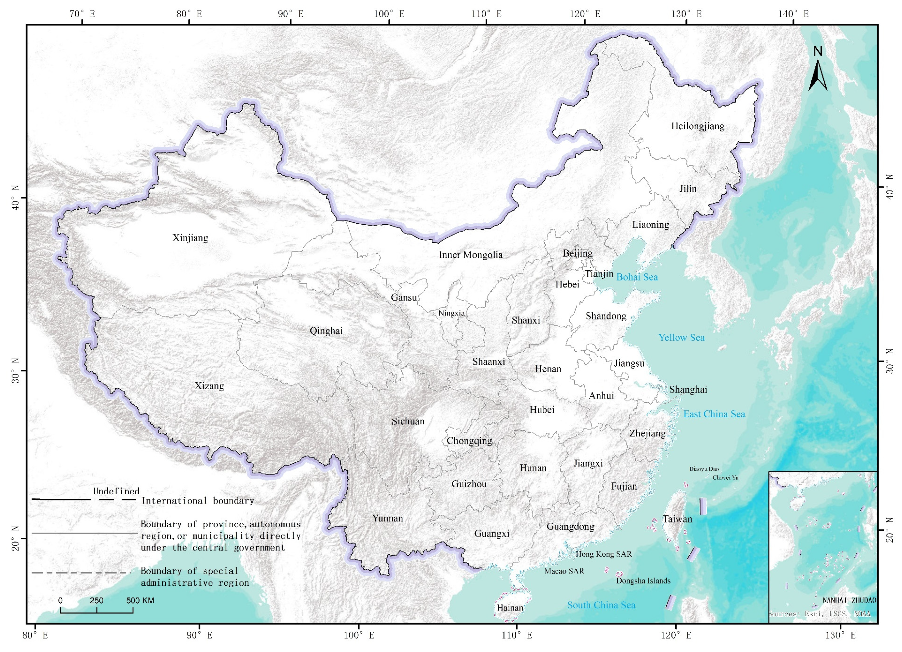
2.1. Study Area

China is located in the eastern part of Asia and on the west coast of the Pacific Ocean. It boasts a vast territory, with a land area of approximately 9.6 million square kilometers and a total sea area of about 4.73 million square kilometers. China’s coastline stretches over 18,000 km, and there are more than 7600 islands distributed within its territorial seas. In terms of land area, China ranks third in the world. It is also the most populous developing country and the second largest economy globally, with rapid GDP growth rate and a continuously optimizing and upgrading economic structure. It has gradually developed from an agriculture-based economy to a diversified one with equal emphasis on industry and service. China is rich in natural resources, enjoys a strategic geographical location, and has a long historical and cultural heritage. Since the reform and opening-up policy, China has undergone rapid development. The continuous optimization and upgrading of its industrial structures have also provided strong support for the sustained and healthy development of the economy. The country has 34 provincial-level administrative regions, including 23 provinces, 5 autonomous regions, 4 municipalities directly under the central government, and 2 special administrative regions. This study takes China as the study area, including Taiwan Province, Hong Kong Special Administrative Region, and Macao Special Administrative Region. The study area is shown in Figure 1.

2.2. Data

The land use data used in this study is further processed based on the 30 m land use data produced by the Chinese Academy of Sciences using Landsat data. This dataset categorizes land use/land cover into six primary classes: cropland, forestland, grassland, water bodies, urban/industrial/mining/residential land, and unused land, with further subdivision into 25 secondary classes. Firstly, data for each land use type was extracted separately to form individual datasets, the data of each land use type was resampled with a resolution of 30 m to 100 m, and the spatial aggregation methods were then used to aggregate the 10 × 10 grids to generate 1 km-gridded products for each land use type, which were subsequently merged into a national 1 km gridded land use dataset. The land use data for the year 2020 was primarily used in this study (Figure 2).

The NTL data used in this study is a global annual “NPP-VIIRS-like” NTL dataset generated by integrating DMSP-OLS NTL and NPP-VIIRS NTL data using a convolutional neural network-based autoencoder model [34]. The spatial resolution of this dataset is 15 arc-seconds (~500 m). The dataset has been validated by the data producers for nighttime light intensity at 150,000 random pixel locations and 40,000 urban areas globally, demonstrating good accuracy at both pixel (R² = 0.87, RMSE = 2.96) and urban (R² = 0.95, RMSE = 3024.62) levels. Therefore, this dataset exhibits excellent spatial patterns and temporal consistency, supporting extended applications across long time series. The NTL data for the year 2020 was primarily used in this study and resampled to a resolution of 1000 m (Figure 2).

The GDP statistical data used in this study mainly involves GDP, value-added of the primary industry (GDP1), secondary industry (GDP2), and tertiary industry (GDP3). These data are primarily sourced from official statistical materials such as provincial and municipal statistical yearbooks, China County Statistical Yearbook, China City Statistical Yearbook, and statistical bulletins. The GDP data for Taiwan, Hong Kong, and Macao are obtained from the official websites of their respective statistical bureaus. Due to differences in official currencies, statistical systems, and statistical methods between Hong Kong, Macao, Taiwan, and the mainland, the industry economic statistics published by these regions were classified into value-added data for the primary, secondary, and tertiary industries according to the Classification Standards for Three Industries published by the National Bureau of Statistics. Furthermore, these data were converted into RMB based on the exchange rates of Hong Kong dollars, Macao patacas, and New Taiwan dollars against RMB in the corresponding historical years to ensure the accuracy and consistency of economic statistical data between Hong Kong, Macao, Taiwan, and the mainland. Ultimately, this study obtained GDP statistical data for 2730 county-level administrative divisions and Taiwan Province, Hong Kong Special Administrative Region, and Macao Special Administrative Region in China for the year 2020 (Figure 3).

3. Methodology

3.1. GDP Modeling Method

GDP is composed of GDP1, GDP2, and GDP3, and the influencing factors for these three industries differ. Therefore, it is necessary to construct gridded models for each of the three industries separately and then combine the gridded results of the value added of the three industries to produce the total GDP gridded product. For the primary industry, it mainly includes economic activities such as agriculture, forestry, animal husbandry, and fishery, which, respectively, correspond to crop land, forest land, grassland, and water areas in land use. And since these production activities are mainly carried out around rural residential areas, correlation analysis is used to verify the degree of correlation between these land use types and the primary industry. The results show (

Table 1. Correlation analysis of modeling factors of the three industries.

	Primary Classification		Secondary Classification	GDP1	GDP2	GDP3
1	Crop land	11	Paddy field	0.59	-	-
		12	Dry land	0.35	-	-
2	Forest land	21	Forest land with trees	0.15	-	-
		22	Shrub land	0.08	-	-
		23	Sparse forest land	-	-	-
		24	Other forest land	0.23	-	-
3	Grassland	31	High-coverage grassland	−0.07	-	-
		32	Medium-coverage grassland	−0.14	-	-
		33	Low-coverage grassland	-	-	-
4	Water and wetland	41	River and canal	0.17	-	-
		42	Lake	−0.05	-	-
		43	Reservoir and pit pond	0.35	-	-
		44	Permanent glacier and snow land	-	-	-
		45	Tidal flat	0.40	-	-
		46	Beach land	-	-	-
5	Construction land	51	Urban land	-	0.81	0.76
		52	Rural residential area	0.53	0.26	0.21
		53	Other construction land	-	0.41	-
6	Unused land	-	-	-	-	-
	NTL	NTL	Nighttime light	-	0.94	0.85

) that crop land, forest land, water areas, and rural residential areas all have a high correlation with the primary industry. Although some land use types such as grassland and lakes do not show a high correlation, considering that grassland and lakes are the main distribution areas for animal husbandry and fishery, respectively, they are also included as modeling factors in the modeling. Therefore, when constructing the spatialization model of the primary industry, crop land, forest land, grassland, water areas, and rural residential areas are mainly used as modeling factors. For the secondary industry, it mainly includes industrial activities such as manufacturing and construction, which mainly correspond to construction land in land use. Therefore, correlation analysis is used to verify the degree of correlation between these land use types and the secondary industry. The results show (Table 1) that urban land, rural residential areas, and industrial and mining land all have a high correlation with secondary industry. Therefore, urban land, rural residential areas, and industrial and mining land are mainly used as modeling factors. For the tertiary industry, it is mainly associated with economic activities related to the service industry. Since service industry activities mainly take place in densely populated areas with a high population density and frequent activities, correlation analysis is used to verify the degree of correlation between urban land, rural residential areas, and the tertiary industry. The results show (Table 1) that both urban land and rural residential areas have a high correlation with tertiary industry. Therefore, urban land and rural residential areas are mainly used as modeling factors. Since economic activities in the primary industry hardly generate significant lighting, the results show (Table 1) that there is a high correlation between NTL and both the secondary and tertiary industries. Therefore, NTL is only used as a modeling factor in the construction of models for the secondary and tertiary industries.

To compare the performance of different models, this study selects four models: linear regression (LR), Random Forest (RF), neural network (NN), and XGBoost, using two modeling approaches, the Factor Averaging Method (FAM) and Grid Averaging Method (GAM) (Figure 4), to construct the GDP spatialization model. Ultimately, the best-fitting model is chosen to spatialize China’s GDP. We aim to complete the construction process of two modeling ideas with the help of four models. We mainly use LinearRegression, RandomForestRegressor, and MLPRegressor from the scikit-learn library, as well as XGBRegressor from the XGBoost library to build these four models. During the model construction process, the dataset is divided into a training set and a testing set at a ratio of 8:2. These four models are, respectively, trained on the training set to enable them to learn the features and patterns in the data. Then, the trained models are used to conduct tests on the testing set to evaluate the performance and generalization ability of the models and thus complete the entire modeling process. Specifically, a linear regression model instance is created using LinearRegression without specifying additional parameters, and the model is trained using the default settings. A Random Forest regression model instance is created using RandomForestRegressor, where the number of decision trees, n_estimators, is set to 100 to ensure that the model has sufficient fitting ability; random_state is used to set the random seed to ensure the reproducibility of the results. A multi-layer perceptron regression model instance is created using MLPRegressor. By setting hidden_layer_sizes = (10, 10, 10), the model is configured to have three hidden layers, with 10 neurons in each hidden layer; max_iter = 1000 specifies the maximum number of iterations for model training; random_state is also used to set the random seed to ensure the reproducibility of model training. An XGBoost regression model instance is created using XGBRegressor. objective = ‘reg:squarederror’ specifies that the objective function for the regression task is the mean squared error; n_estimators = 160 indicates that the number of decision trees to be trained is 160; learning_rate = 0.1 controls the contribution degree of each tree; max_depth = 9 specifies the maximum depth of the decision trees; random_state is used to set the random seed.

FAM involves using the area proportion of each modeling factor to the total sum of all modeling factors as the independent variable and taking the average value of industrial added value over the total area of all relevant modeling factors as the dependent variable. Models are constructed at county-level administrative units and then applied to a 1 km grid scale to obtain 1 km gridded products. The formulas are as follows:

$F_i$ represents the area of the i-th modeling factor, $F_{total}$ represents the total area sum of all modeling factors for each industry, and $Y_j$ represents the industrial value added to the j-th county-level administrative unit.

The independent variable (factor area ratio) is

$$X_{i,j}={\displaystyle \frac{F_i}{{\sum }_k{F}_k}}={\displaystyle \frac{F_i}{F_{total}}}$$

(1)

The dependent variable (the average value of industrial added value in the total area of the factors) is

$${\overline{Y}}_j={\displaystyle \frac{Y_j}{\sum _i{F}_i}}={\displaystyle \frac{Y_j}{F_{total}}}$$

(2)

The model constructed at the county-level administrative unit can be expressed as

$${\overline{Y}}_j=f(X_{1,j},X_{2,j},\dots ,X_{n,j})$$

(3)

where f represents the constructed model function and n represents the number of modeling factors.

GAM involves taking the average area of each modeling factor distributed across the grid as the independent variable, and using the average value of industrial added value on the grid as the dependent variable. Models are constructed at county-level administrative units and then applied to a 1 km grid scale to obtain 1 km gridded products. The formulas are as follows:

$F_i$ represents the area of the i-th modeling factor, $F_{grid}$ represents the total area sum of all grids within the county-level administrative unit, and $Y_j$ represents the industrial value added of the j-th county-level administrative unit.

The independent variable (the average area of the factor on the grid) is

$${\overline{X}}_{i,j}={\displaystyle \frac{F_i}{F_{grid}}}$$

(4)

The dependent variable (the average value of industrial added value on the grid) is

$${\overline{Y}}_j={\displaystyle \frac{Y_j}{F_{grid}}}$$

(5)

The model constructed at the county-level administrative unit can be expressed as

$${\overline{Y}}_j=g({\overline{X}}_{1,j},{\overline{X}}_{2,j},\dots ,{\overline{X}}_{n,j})$$

(6)

where g represents the constructed model function and n represents the number of modeling factors.

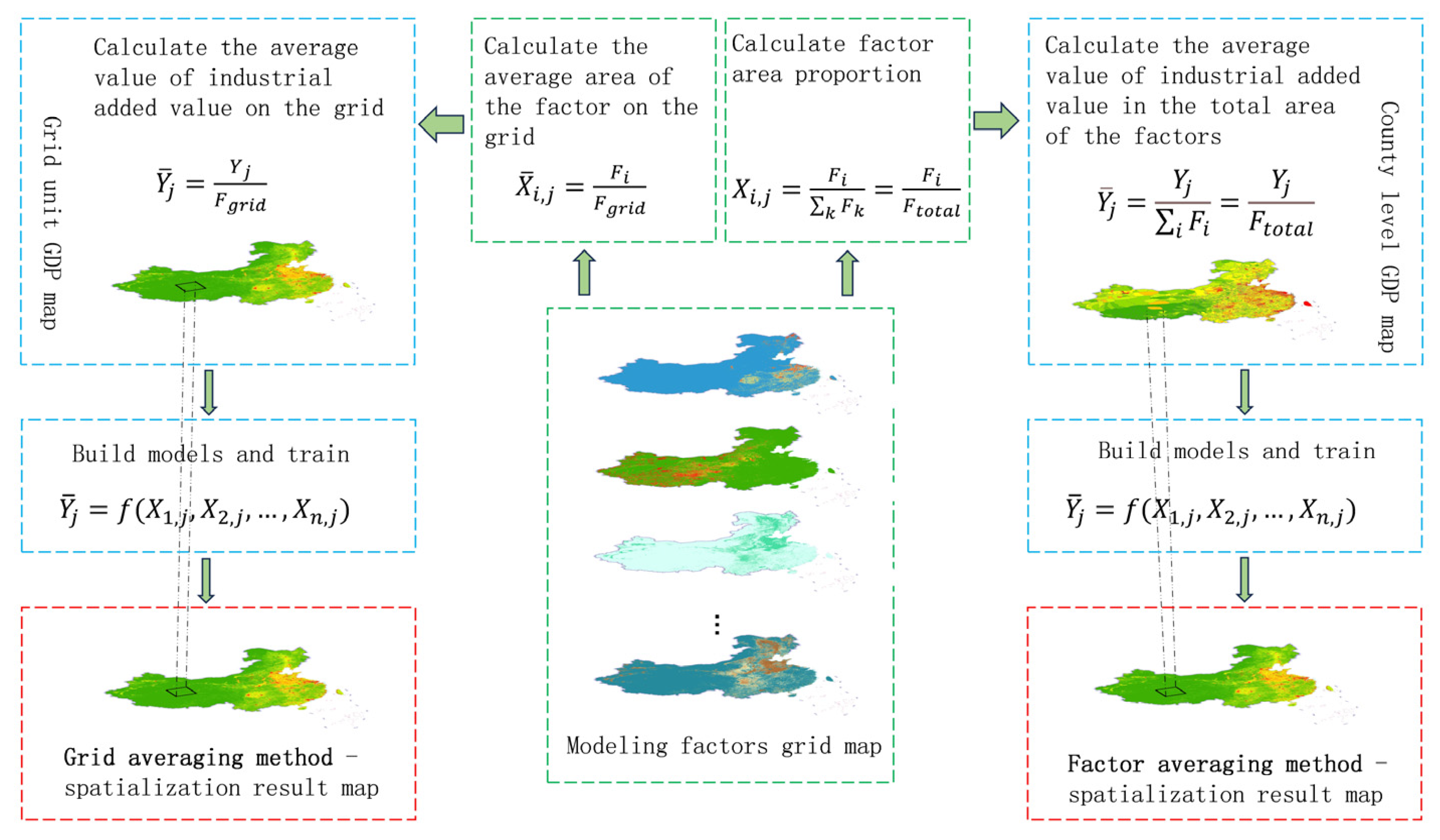
3.2. GDP Spatialization

The optimal model with the highest accuracy is applied to 1 km resolution gridded variables to produce a spatial gridded distribution map of GDP in China. Due to the errors inherent in the fitted model, there will inevitably be a deviation between the predicted GDP values and actual statistical values of GDP in some counties. Therefore, it is necessary to use county-level GDP statistical data to perform a linear correction on the predicted GDP values, ensuring effective control of errors within county boundaries and the accuracy of the prediction results [35]. The following formula is used to correct the predicted GDP on a grid-by-grid basis:

$${GDP}_c={GDP}_e\ast {\displaystyle \frac{{GDP}_s}{{GDP}_p}}$$

(7)

where ${GDP}_C$ represents the corrected GDP for a grid unit, ${GDP}_e$ represents the predicted GDP for a grid unit before correction, ${GDP}_s$ represents the county-level GDP statistical data, and ${GDP}_p$ represents the predicted county-level GDP.

The total GDP for the entire study area is obtained by spatially aggregating the prediction results from the models for the three industries. This process can be expressed as

$${{GDP}_j={GDP1}_j+GDP2}_j+{GDP3}_j$$

(8)

where ${GDP}_j$ represents the GDP of the j-th grid unit, ${ GDP1}_j$ represents the value added of the primary industry for the j-th grid unit, ${GDP2}_j$ represents the value added of the secondary industry for the j-th grid unit, and ${GDP3}_j$ represents the value added of the tertiary industry for the j-th grid unit.

3.3. Accuracy Assessment

In order to evaluate the performance and accuracy of the model in terms of GDP spatialization, the coefficient of determination (R²) from the regression model is utilized to assess the goodness-of-fit of the model’s GDP spatial distribution. This indicator directly reflects the strength of the linear relationship between the model’s predicted values and the actual statistical values. Additionally, the Root Mean Square Error (RMSE) and Mean Absolute Error (MAE) are calculated to further evaluate the model’s accuracy. These two indicators quantify the model’s prediction precision from two dimensions: overall error level and average error level. The RMSE is more sensitive to outliers and can reflect the overall variability of the model’s predictions, while the MAE provides a measure of the average deviation of the model’s predictions. Moreover, to further enhance the validity of the evaluation, town-level GDP statistical data are also used to assess the accuracy of the spatialized results.

$$R^2=1-{\displaystyle \frac{{\sum }_{i=1}^N{({GDP}_s-{GDP}_p)}^2}{\sum _{i=1}^N{({GDP}_s-\overline{{GDP}_s})}^2}}$$

(9)

$$RMSE=\sqrt{{\displaystyle \frac{1}{N}}{\sum }_{i=1}^N{({GDP}_s-{GDP}_p)}^2}$$

(10)

$$MAE={\displaystyle \frac{1}{N}}{\sum }_{i=1}^N\left|{GDP}_s-{GDP}_p\right|$$

(11)

where ${GDP}_s$ represents the true statistical value of GDP, ${GDP}_p$ represents the predicted value of GDP, and N represents the number of samples.

4. Results

4.1. Model Performance Evaluation

For the two methods of FAM and GAM, we compared the performance of four models: LR, RF, NN, and XGBoost, as shown in

Table 2. Performance comparison of models in FAM.

	Model	R2	MAE	RMSE
GDP1	Linear regression	0.16	0.02	0.04
	Random Forest	0.64	0.01	0.02
	Neural network	0.19	0.02	0.04
	XGBoost	0.74	0.01	0.02
GDP2	Linear regression	0.15	1.14	2.27
	Random Forest	0.71	0.60	1.34
	Neural network	0.16	1.14	2.27
	XGBoost	0.78	0.35	1.16
GDP3	Linear regression	0.42	1.93	4.90
	Random Forest	0.71	0.91	3.44
	Neural network	0.47	1.70	4.66
	XGBoost	0.63	0.65	3.88

and

Table 3. Performance comparison of models in GAM.

	Model	R2	MAE	RMSE
GDP1	Linear regression	0.32	0.91	1.88
	Random Forest	0.83	0.41	0.94
	Neural network	0.52	0.88	1.58
	XGBoost	0.87	0.20	0.83
GDP2	Linear regression	0.55	16.66	58.63
	Random Forest	0.82	8.41	36.92
	Neural network	0.55	16.48	58.46
	XGBoost	0.87	4.55	31.33
GDP3	Linear regression	0.50	113. 08	335.88
	Random Forest	0.87	26.00	174.09
	Neural network	0.58	60.67	306.39
	XGBoost	0.66	32.11	276.43

. The results indicate that different methods and models have varying impacts on the outcomes. In the FAM, the optimal R² values for GDP1, GDP2, and GDP3 were 0.74, 0.78, and 0.71, respectively. In the GAM, the optimal R² values for GDP1, GDP2, and GDP3 were 0.87, 0.87, and 0.87, respectively. Moreover, the R² values of all models for the three industries in the GAM were higher than those in the FAM, suggesting that the modeling approach of GAM is superior to that of FAM. Among the four models, RF and XGBoost exhibited significantly better modeling performance than LR and NN, indicating that machine learning models are more suitable than linear regression and neural network models for constructing GDP spatialization models. Furthermore, for GDP1 and GDP2, XGBoost had higher R² values than RF, demonstrating better modeling performance. However, for GDP3, RF showed better modeling performance than XGBoost.

Therefore, we selected the modeling method with better performance, namely GAM, as the foundation for GDP spatialization. Specifically, we employed the XGBoost model for GDP1 and GDP2 spatialization, and the RF model for GDP3 spatialization. Finally, the total GDP spatialization result was obtained by summing the outputs of these three spatialization models. To validate the modeling effectiveness of this model combination, we conducted an accuracy assessment using town-level GDP statistical data.

4.2. Accuracy Assessment at Town-Level

To evaluate the accuracy of the GDP spatialization model, it is common practice to compare the finer-scale town-level GDP statistical data with the corresponding aggregated town-level GDP data estimated from the gridded GDP data. However, due to the Chinese government’s lack of plans to release town-level GDP statistical data, such data are generally unavailable for most towns. We have made every effort to collect GDP statistical data for 110 township levels from the 2020 Statistical Yearbook to assess the accuracy of the gridded total GDP results obtained using this combined modeling approach. The results (

Table 4. Accuracy assessment of model combination method at town-level.

	R2	MAE	RMSE
RF + XGBoost	0.78	37.96	60.03

) show that this combined method performs well on the town-level validation dataset, with an R² of 0.78, indicating its reliable prediction capability, and relatively small MAE and RMSE values. Therefore, the gridded total GDP results obtained by using the XGBoost model for GDP1 and GDP2 spatialization and the RF model for GDP3 spatialization have good accuracy.

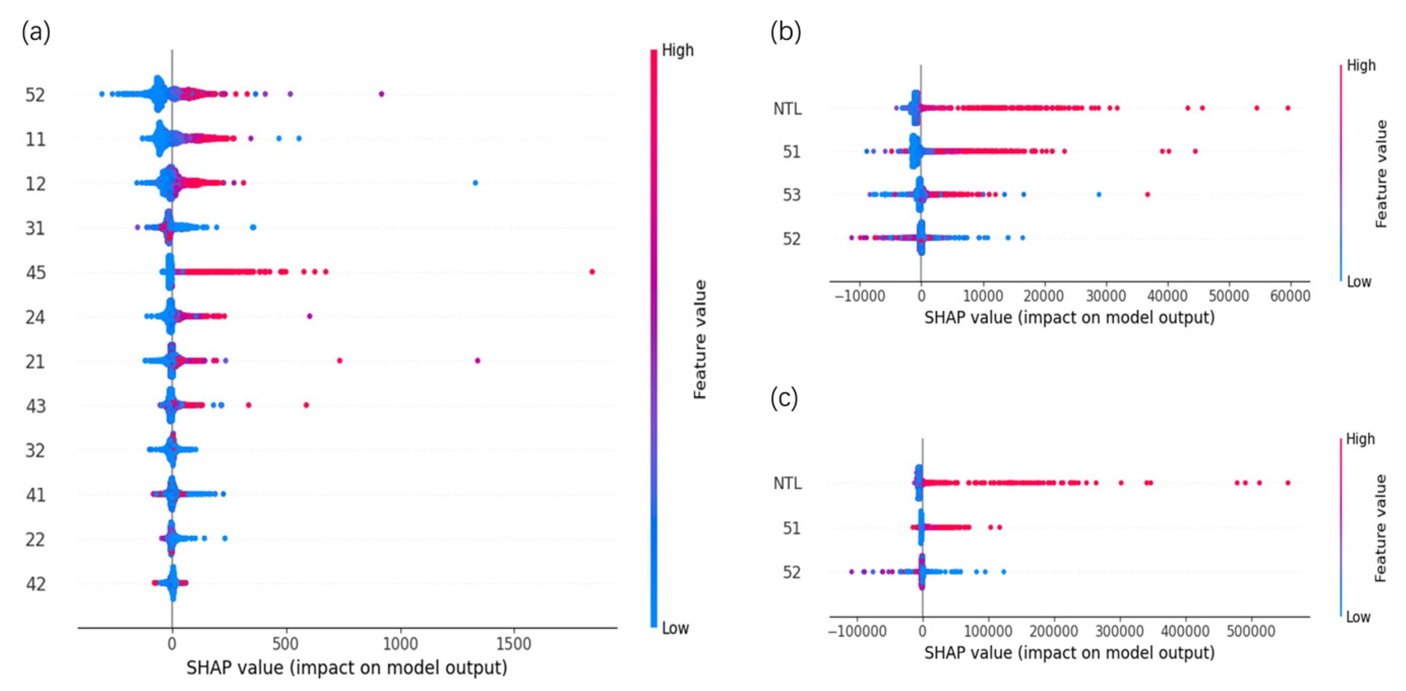
4.3. Feature Importance Analysis

SHAP (SHapley Additive exPlanation) provides a unified framework for explaining the predictions of machine learning models and analyzing the marginal contributions of features to the prediction results [36]. Here, we utilize SHAP to evaluate the feature importance in the XGBoost model for the primary and secondary industries and in the RF model for the tertiary industry, with the aim of identifying the key factors driving the prediction accuracy.

As can be seen from Figure 5a, the points of the feature “52” (rural residential areas) are distributed over a wide range, and there are many points with large absolute values of SHAP values. This indicates that “52” has a more significant impact on the model output compared to other features, making it a relatively important feature. Following it are “11” (paddy field) and “12” (dry land), which strongly prove that crop land occupies a dominant position in the production activities of the primary industry and is the main driving force for the development of the primary industry. The points “45” (tidal flat) and “24” (other forest land) also exhibit relatively high feature values, suggesting that tidal flat and other forest land make relatively high contributions to the primary industry.

As can be seen from Figure 5b, the points of the “NTL” feature are widely distributed and the SHAP values vary greatly, indicating that the “NTL” feature has the greatest impact on the model output. In contrast, the distribution ranges and variation amplitudes of the SHAP values of “51” (urban land), “53” (other construction land), and “52” (rural residential area) are relatively small, and their importance gradually decreases.

As can be seen from Figure 5c, “NTL” is still a relatively important feature, with a large distribution range of its points and a large degree of variation in SHAP values. The distribution of SHAP values of the features “51” (urban land) and “52” (rural residential area) is relatively concentrated, and their importance is lower than that of “NTL”.

4.4. GDP Spatialization Results

China’s 1 km gridded GDP in 2020 is shown in Figure 6, which clearly reveals the regional characteristics of China’s economic development. The results show that China’s GDP is predominantly concentrated in the plains and hilly regions on the southeast side of the “Hu Huanyong Line” (Hu Line), with only a minor portion distributed in the grasslands and deserts regions on the northwest side of the Hu Line. Specifically, relatively high GDP values are mainly distributed in the Huang–Huai–Hai Plain and the eastern coastal areas, while relatively low GDP values are mainly distributed in most areas of Tibet, Qinghai, Xinjiang, and inner Mongolia, which reflects the spatial imbalance of economic activities. Four representative regions are enlarged and further analyzed for their GDP spatial distribution: Chengdu–Chongqing (CC), Beijing–Tianjin–Hebei (BTH), the Pearl River Delta (PRD), and the Yangtze River Delta (YRD). These are China’s four largest urban agglomerations and also regions with robust economic development. It can be seen that the BTH has significantly more high-value GDP grids, indicating a relatively high level of economic development. Especially in Beijing, Tianjin, and their surrounding areas, economic activities are dense. The YRD also has a large area where high-value GDP grids gather. With a complete industrial system and strong economic vitality, it makes a significant contribution to the national GDP and is one of the most economically developed regions in China. The PRD is also an area where high-value GDP grids cluster. Its manufacturing industry, service industry, and foreign trade and other industries are well-developed. It is a highly developed economic region, and its GDP level is leading in the country. The CC has a relatively large number of high-value GDP grids, indicating that this region is an economically developed area in the central and western regions of China and plays an important leading role in regional economic development. It is evident that the GDP level in BTH, PRD, and YRD is significantly higher than that in CC, and the urban agglomeration’s synergistic development effect is better pronounced among the former three. Upon closer inspection, urban centers such as Beijing, Shanghai, Guangzhou, and Shenzhen exhibit more high-value GDP grids (exceeding 100 million yuan) than other urban centers. As one moves outward from these central cities, the number of high-value GDP grids gradually decreases, displaying a trend of diminishing values from the center to the periphery. This demonstrates that cities serve as the primary carriers of economic activities, and there exists a strong positive correlation between the level of urbanization and the GDP level. Additionally, high-value GDP grids are primarily distributed in the urban centers of economically developed provinces and cities, exhibiting a dispersed, dot-like spatial distribution overall. These high-value GDP grids are typically surrounded by secondary-level GDP grids, and the values of GDP grids decrease progressively with increasing distance from the urban center. From the coastal areas to inland, the GDP values show a certain gradient of decreasing. The coastal areas have a relatively high level of economic development, and as one moves closer inland, the level of economic development gradually decreases. The grids with low GDP values are mainly concentrated in the northwestern regions such as Tibet, Qinghai, Xinjiang, and inner Mongolia. The spatial distribution of gridded total GDP data are logically highly consistent with the basic distribution pattern of China’s mainland GDP, indicating the effectiveness of the proposed GAM and model combination approach.

4.4.1. Primary Industry Spatialization Results

China’s 1 km gridded GDP1 product in 2020 is shown in Figure 7, which clearly reveals the spatial distribution of agricultural economic activities in China. The results show that the gridded GDP1 is generally distributed throughout China, with a concentration in the plains and hilly regions on the southeast side of the Hu Line; this is related to the relatively superior natural conditions, more complete agricultural infrastructure and market conditions in the eastern regions, and only minimal distribution in the grasslands and deserts regions on the northwest side of the Hu Line. This distribution pattern aligns with the spatial distribution of China’s 1 km gridded total GDP. Compared with the inland areas, there are more grids with relatively high GDP values in the coastal areas. This is because the coastal areas enjoy convenient transportation, which is conducive to the transportation and sales of agricultural products. At the same time, they have advantages in some aspects, such as in the promotion of agricultural technologies and marine fishery. Furthermore, since the primary industry is closely related to agricultural activities, its spatial distribution pattern is consistent with the distribution of crop land cover, reflecting the spatial distribution characteristics of agricultural production. Similarly, by zooming in on the four largest urban agglomerations in China—CC, BTH, PRD, and YRD—and further analyzing the spatial distribution of GDP1, it can be seen that low-value GDP grids are distributed in the urban centers of Beijing and Tianjin, while relatively high-value GDP grids are distributed in their surrounding areas. This may be due to the large demand for agricultural products in the cities, which has driven agricultural production and development in the surrounding areas. The primary industry in the YRD has a relatively high GDP level. Here, the degree of agricultural modernization is high, and the development of high-efficiency agriculture and characteristic agriculture is relatively good. At the same time, related production activities such as fishery also have a certain scale. The primary industry in the PRD also has a good development situation. The suitable climate and geographical conditions make the agricultural fields with high economic value, such as flower cultivation and fruit and vegetable production, perform outstandingly. The CC is an area where the primary industry is relatively developed in the central and western regions. It has suitable climatic conditions and a good agricultural foundation. In urban center areas, due to accelerated urbanization, agricultural land has decreased relatively, leading to a higher concentration of low-value GDP grids (less than 1 million RMB). Conversely, in suburban and rural areas of cities, it is likely that due to the huge demand for agricultural products from cities, the agricultural production in the surrounding areas has been stimulated, and suburban agriculture has been developed. As a result, agricultural activities remain prosperous, and thus there are more GDP grids with high values (exceeding 5 million RMB). This trend is most significant in the CC, PRD, and YRD regions. Areas with richer agricultural activities have higher-value GDP grids, indicating a positive correlation between the two. However, there are very few GDP grids exceeding 100 million RMB, suggesting that the economic value generated by agricultural activities has a certain upper limit. Since agricultural activities are mainly distributed outside urban centers, the high-value GDP grids of the primary industry are correspondingly concentrated in these areas, indicating that the spatial distribution of the gridded GDP1 is reasonable. Nevertheless, when compared with the gridded total GDP in Figure 6, the majority of GDP grids in the primary industry have relatively lower values overall. This is both consistent with the economic characteristics of agricultural activities and reflects the differences between agriculture and industry/services within China’s industrial structure, aligning with real-world conditions.

4.4.2. Secondary Industry Spatialization Results

China’s 1 km gridded GDP2 in 2020 is shown in Figure 8, which clearly reveals the spatial distribution of industrial economic activities in China. The results indicate that the gridded GDP2 is also predominantly concentrated in the plains and hill regions on the southeast side of the Hu Line, with minimal distribution in the grasslands and desert regions on the northwest side of the Hu Line. This distribution pattern is consistent with the spatial distribution of China’s 1 km gridded total GDP. Moreover, the eastern and coastal regions have formed obvious industrial agglomeration advantages, presenting a spatial distribution pattern where the east is stronger than the west. This is related to factors such as convenient transportation, foreign trade, port transportation, and industrial foundation in the eastern and coastal regions, which are conducive to the development of the secondary industry, such as the manufacturing industry and port-related industries. Given that the secondary industry is closely tied to industrial activities, its spatial distribution aligns well with the spatial distribution of industrial and mining land, reflecting the dependency of industrial development on geographical conditions. Regions with richer industrial activities tend to have higher-value GDP grids, and these relatively high-value GDP grids are mainly scattered around the peripheries of major cities, particularly in suburban areas, with only a small portion located in urban centers. Similarly, by zooming in on the four largest urban agglomerations in China—CC, BTH, PRD, and YRD—and further analyzing the spatial distribution of GDP2, it can be seen that the development level of the secondary industry in the BTH is relatively high. In particular, Beijing and Tianjin, as important industrial and manufacturing bases, have a complete range of industrial categories, and high-tech industries and high-end manufacturing industries are developing rapidly. The YRD is a high-value aggregation area of the GDP of the secondary industry. The region has a complete industrial system, with layouts ranging from traditional manufacturing industries to advanced manufacturing industries and strategic emerging industries. It is an important manufacturing and industrial innovation center in China. The development of the secondary industry in the PRD is extremely active. With industries such as electronic information, home appliance manufacturing, and automobiles as its pillars, it occupies an important position in the global industrial chain, has a complete industrial supporting system, and strong innovation capabilities. The CC is a relatively developed area of secondary industry in the central and western regions. It has a certain scale and competitiveness in industries such as equipment manufacturing, electronic information, and automobiles, and is an important industrial base in the central and western regions. In comparison, the PRD region has the highest number of high-value GDP grids, followed by the YRD and BTH regions. The CC region has the relatively lowest number of high-value GDP grids among the gridded GDP2. Even so, the distribution of the GDP2 in the YRD region is more uniform compared to the other three zoomed-in areas, suggesting a more stable and balanced industrial economic development in this region. Since industrial activities typically require numerous industrial facilities and occupy a large area, they often tend to be located in suburban areas. Therefore, the spatial distribution of the gridded GDP2 is reasonable.

4.4.3. Tertiary Industry Spatialization Results

China’s 1 km gridded GDP3 product in 2020 is shown in Figure 9, which clearly reveals the spatial distribution of service economic activities in China. The results indicate that the gridded GDP3 is also predominantly concentrated in the plains and hill regions on the southeast side of the Hu Line, with minimal distribution in the grasslands and deserts regions on the northwest side of the Hu Line. The southeast side features a dense population, a high level of urbanization, and large market demand, which provides a favorable environment for the development of tertiary industry. Restricted by factors such as geography, population, and economic foundation, the development of tertiary industry on the northwest side is relatively lagging behind. This distribution pattern is consistent with the spatial distribution of China’s 1 km gridded total GDP. Moreover, obvious economic agglomeration areas have been formed in the eastern and coastal regions, presenting a spatial distribution pattern where the east is higher than the west, which reflects the fat that the eastern and coastal regions have significant advantages in the development of tertiary industry, such as commerce, finance, and scientific and technological services. Given that the tertiary industry is closely tied to service activities, its spatial distribution aligns well with the spatial distribution of the population. The more densely populated regions are often accompanied by more abundant service industry activities, resulting in higher-value GDP grids. These relatively high-value GDP grids are also mainly concentrated around large cities, particularly in urban centers, reflecting the strong dependence of the service industry on population agglomeration. Similarly, by zooming in on the four largest urban agglomerations in China—CC, BTH, PRD, and YRD—and further analyzing the spatial distribution of GDP3, it can be seen that the tertiary industry in the BTH is booming. As the capital of China, Beijing takes the lead in high-end service sectors such as finance, technology, and cultural and creative industries. Relying on its port advantages, Tianjin stands out in logistics, trade, and other fields. The YRD is a high-value aggregation area of the GDP of the tertiary industry. The region is home to international financial, trade, and shipping centers like Shanghai. Meanwhile, the service industries in cities such as Nanjing and Hangzhou are also highly developed, forming a complete industrial ecosystem and a pattern of coordinated development. The development of the tertiary industry in the PRD is also very active. Centered around Guangzhou and Shenzhen, it has developed rapidly in fields such as Internet services, financial technology, business, and trade exhibitions. It develops in coordination with the manufacturing industry, promoting the high-quality development of the regional economy. The CC is a relatively developed area of the tertiary industry in the central and western regions of China. As regional central cities, Chengdu and Chongqing have strong radiation and driving capabilities in consumption, finance, tourism, and other aspects, which have promoted the development of the tertiary industry in the surrounding areas. In comparison, the PRD region has the highest number of high-value GDP grids, followed by the YRD and BTH regions. The CC region has the relatively lowest number of high-value GDP grids among the gridded GDP3. It is also found that the distribution of GDP3 in the YRD region is more balanced compared to the other three zoomed-in areas, indicating a more comprehensive and stable development of the service industry in this region. Urban centers, such as Chengdu, Chongqing, Beijing, Tianjin, Guangzhou, Shenzhen, Nanjing, and Shanghai, typically have higher-value GDP grids. These centers have higher population densities, more concentrated populations, better consumption capacity and infrastructure, and richer and more frequent service activities, which provide the necessary conditions for the development of the tertiary industry. Therefore, the spatial distribution of the gridded GDP3 is reasonable. Compared to the gridded GDP2 in Figure 8, the gridded GDP3 is more concentrated in spatial distribution and has more high-value GDP grids overall. This difference not only reflects the different characteristics of the spatial layout between the service industry and the industrial industry but also reveals the rise in the service industry and its significant contribution to economic growth during China’s economic structural transformation.

5. Discussion

5.1. Comparison with Publicly Available GDP Datasets

This study maps the spatial grid distribution of China’s GDP based on remote sensing data and machine learning methods and evaluates its accuracy using town-level GDP statistical data. The results indicate that the GDP spatialization obtained through this method exhibits good accuracy. Furthermore, it is compared with publicly available GDP datasets. However, most studies are limited to specific research areas, such as coastal areas [22,26], urban agglomerations [28], provincial administrative regions [24], or prefecture-level cities [23,29]. Although many studies take China as the research area, the spatialized result data are not fully publicly available, and the original result data for comparison cannot be obtained. Therefore, limited by the inconsistent scope and time of some current GDP datasets, we selected the Xu_GDP dataset for the year 2020, also with the same resolution of 1 km (https://www.resdc.cn/DOI/doi.aspx?DOIid=33, accessed on 25 February 2025), for comparison. Figure 10 displays the 2020 Xu_GDP dataset of China at a 1 km grid resolution, which overall exhibits a consistent spatial distribution pattern and aggregation trend, shown in Figure 6. Specifically, China’s GDP is predominantly distributed on the southeast side of the Hu Line, with minimal distribution on the northwest side of the Hu Line. Relatively higher GDP values are concentrated in the Huang–Huai–Hai Plain and eastern coastal areas, while relatively lower GDP values are mainly distributed in most areas of Tibet, Qinghai, Xinjiang, and inner Mongolia. It is also evident that although both datasets have a 1 km resolution, compared to Figure 6, the Xu_GDP dataset shows more prominent administrative boundary effects, failing to detail the differences within county-level administrative units. This may lead to an overestimation of non-urban areas to some extent, indicating a slightly lower level of refinement compared to our GDP dataset.

To further compare the spatialized GDP results obtained using traditional statistical model methods and machine learning methods, we conducted a comparison with the HXD_GDP dataset derived from the statistical model proposed by Han et al. [37]. Figure 11 displays the spatial distribution of the 1 km gridded HXD_GDP dataset for China in 2020, which overall exhibits a spatial distribution pattern and aggregation trend consistent with Figure 6. This comparison further validates the validity and reliability of our dataset (OUR_GDP). For a more detailed comparison between the two datasets, we conducted local enlargements and in-depth analyses of four key economic regions: CC, BTH, PRD, and YRD (Figure 12). The results revealed that the spatialized GDP results of the two datasets are highly consistent in terms of the overall distribution pattern. Both show a trend of gradually decreasing GDP values from the economic center to the periphery, reflecting the economic radiation effect of the economic center on the surrounding areas. The spatial patterns of economic development levels are highly similar, indicating that both datasets can reflect the agglomeration characteristics of economic activities in key economic regions. However, the GDP distribution of the HXD_GDP dataset exhibits more pronounced fragmentation, particularly in the YRD. In contrast, the distribution of OUR_GDP is smoother, better reflecting the gradual decrease in high-value GDP to low-value GDP in the process of diffusion from central cities to surrounding cities, thus demonstrating superior spatial continuity. Additionally, we also evaluated the accuracy of the HXD_GDP dataset using town-level GDP statistical data, with results showing an R² of 0.68, and MAE and RMSE of 44.20 and 72.75, respectively. Comparing these evaluation results with Table 4, it is evident that OUR_GDP exhibits higher accuracy (R² = 0.78) and lower MAE and RMSE values, demonstrating the precision advantage of the OUR_GDP dataset. Therefore, the spatialized GDP results obtained using the machine learning method in this study not only maintain consistency with the statistical modeling method in terms of spatial distribution patterns but also exhibit improvements in spatial continuity and accuracy.

5.2. Comparison of Modeling Methods

With the advancement of technology, the modeling methods for GDP spatialization have been continuously optimized and improved. Initially, scholars discovered a close relationship between NTL and economic activity [14,38]. The strong correlation between the two made it possible to use NTL to characterize the status of economic activities, thereby initiating the development and refinement of GDP spatialization methods. Initially, traditional linear regression models were used to quantify the regression relationship between NTL data and GDP [17]. However, NTL data could never serve as the sole source for regional economic modeling. As such, scholars began to incorporate data closely related to socio-economic activities, such as land use data [22,24] and demographic data [15], into the construction of spatialization models. For regions with prominent spatial heterogeneity, methods such as the dynamic regional approach and zoning modeling were used to construct separate spatialization models for each subregion to improve the accuracy of the results [22]. In order to produce higher-resolution GDP spatial grid products, the use of NTL data alone has become insufficient to meet modeling requirements. Therefore, scholars have gradually incorporated high-resolution optical imagery [29], POI data [28], Tencent user density data [7], industrial entity big data [39], road density data [10], land surface temperature data [23], and other auxiliary data into GDP spatialization modeling. The increase in auxiliary modeling data has made it difficult for linear regression models to capture the complex relationships between GDP and these various auxiliary data. Consequently, machine learning methods such as RF and XGBoost [9,26,27] have been widely applied in GDP spatialization modeling. Moreover, with the continuous development of deep learning, some scholars have also used deep learning approaches to develop GDP spatialization models [10,28,33]. The powerful learning capabilities of these methods enable them to effectively capture the complex relationships between auxiliary modeling data and GDP, demonstrating better performance than simple linear or nonlinear regression algorithms. However, deep learning often requires higher performance hardware support, more complex model design and more modeling samples. In contrast, machine learning is relatively simple and easy to use, and can efficiently process large-scale datasets. Since this study does not involve a vast amount of auxiliary modeling data, and machine learning algorithms can achieve good model performance, it is appropriate to use machine learning algorithms such as RF and XGBoost to construct GDP spatialization models in this study.

Regarding the two modeling methods, FAM and GAM, the former takes the area proportion of each modeling factor to the total sum of all modeling factors as the independent variable, while the latter uses the area of each modeling factor averaged over the grid as the independent variable. The FAM can effectively reflect the influence weight of each modeling factor on industrial value-added weight and better demonstrate the relative importance among factors. However, it involves more complex mathematical calculations, which may lead to higher computational complexity for large areas or finer grid scales, increasing the difficulty of model construction. Additionally, it may fail to fully capture the differences and changes in local areas. In contrast, the GAM is relatively simple to calculate. Especially at higher resolutions, it can directly use the grid’s average value as the factor input without additional proportional adjustments, making it suitable for applications at various spatial scales with good adaptability and flexibility. It also provides a more detailed reflection of local changes and differences, helping to reveal the subtle characteristics of spatial distribution. Therefore, in this study, the GAM is used as the basis for constructing the GDP spatialization model.

5.3. Comparison of the Three Industries

Constructing spatialization models separately for the three industries rather than for total GDP has been performed due to the distinct spatial distribution characteristics of economic activities across different industries, which result in the use of different auxiliary data for modeling. Primary industry is closely related to farmland, forests, grasslands, inland freshwater, and marine aquaculture. Secondary industry has a high correlation with urban areas, rural settlements, industrial parks, and mining areas. Tertiary industry is closely linked to urban and rural settlements where service industries are abundant and populations are concentrated. Furthermore, since economic activities in the primary industry rarely generate significant amounts of light, NTL data are only used as a modeling factor in the construction of models for the secondary and tertiary industries. This approach allows a more accurate spatialization of the output value of each industry, and captures the nuances of their respective economic activities and spatial distribution. By modeling each industry separately, we can better understand and express the contribution of different industries to the overall economic output.

As shown in Figure 7, Figure 8 and Figure 9, on the whole, primary industry has more low-value GDP grids compared to secondary and tertiary industries, and tertiary industry has more high-value GDP grids than secondary industry, with these high-value areas being more concentrated in urban centers. Primary industry is predominantly located outside of urban centers, particularly in suburban and rural areas, which aligns with the reality that agricultural-related activities tend to be situated away from densely populated urban cores. Both secondary and tertiary industries are primarily distributed in and around large cities, but they exhibit distinct spatial patterns. Secondary industry is more prominent in suburban areas, whereas tertiary industry dominates urban centers. This distribution aligns well with the fact that a multitude of service-related activities are concentrated in city-center areas. The spatial distribution differences observed in the gridded GDPs among the three industries are consistent with the actual distribution of real GDP. This consistency not only validates the accuracy and reliability of the employed spatialization models but also successfully captures the spatial distribution and geographical concentration of economic activities for each industry.

5.4. Limitations and Future Work

Despite having established spatialized models for the three industries based on their respective relevant modeling factors and achieving satisfactory model results, land use data solely reveals the type of land use without accurately depicting the density or quality of economic activities on the land. Consequently, relying solely on land use data to construct a spatialized model for primary industry may lead to overestimation of economic activities in some areas and underestimation in others. Similarly, solely using land use data and NTL remains challenging in clearly distinguishing between the secondary and tertiary industries, as the spatial distributions and economic activity characteristics of these two industries sometimes exhibit significant overlap. The secondary industry, particularly manufacturing, is typically concentrated in industrial parks or factory zones, which may exhibit similar NTL intensities to commercial and service areas belonging to the tertiary industry. Furthermore, high-end service sectors within the tertiary industry, such as finance and technology, may exhibit lighting patterns that are relatively close to those of traditional industrial areas in some regions, making it difficult to distinguish between these two types of industries solely based on NTL data. Additionally, with the acceleration of urbanization, some areas originally dominated by the secondary industry may gradually transition to being dominated by the tertiary industry, a transformation that may not be evident in land use and NTL data. Therefore, to more accurately distinguish between the secondary and tertiary industries, it is beneficial to integrate data that can represent economic or human activity status, such as POI [21], big data on industrial and commercial enterprises [39], and Tencent user density [7], which can help differentiate the economic activity characteristics of different industries [40]. Meanwhile, using high-resolution remote sensing imagery to conduct more detailed classification and identification of land use types can also enhance the accuracy and reliability of industrial spatialized models.

Although RF and XGBoost algorithms have been able to establish a good GDP spatialization model in this study, deep learning methods, especially convolutional neural networks (CNNs), recurrent neural networks (RNNs), and other advanced models, still have great potential and advantages. These methods can extract more complex features from multi-source data, especially demonstrating stronger expressive power when dealing with nonlinear and high-dimensional data. This offers new possibilities for further improving model prediction accuracy and generalization ability. Compared with traditional machine learning algorithms, deep learning has significant advantages in processing complex spatial data and capturing potential spatial dependencies, thanks to its powerful feature extraction and nonlinear mapping capabilities [10,33]. Therefore, future research can more effectively integrate deep learning techniques into GDP spatialization modeling by constructing end-to-end deep learning models, combined with advanced model optimization strategies and large-scale data processing technologies. The goal is to achieve higher prediction accuracy and stronger model interpretability, providing more scientific and precise decision support for regional economic development planning and policy formulation.

The reliability of spatialized GDP results largely depends on the quality of statistical data. The small amount of GDP statistics at the county level may contain errors, potentially due to intentional manipulation [4]. Furthermore, there is no unified standard for GDP statistics across provinces and municipalities in China, making the acquisition process time-consuming and laborious. Additionally, the incomplete GDP statistics at the township level further complicate the accuracy assessment [28]. Therefore, achieving high-resolution GDP grid mapping remains a challenging task. In order to obtain more accurate spatialized GDP results, it is still necessary to collect ground observation data with higher resolution.

6. Conclusions

This study employed land use and NTL remote sensing data, using the GAM as the foundation for GDP spatialization modeling, by leveraging RF and XGBoost algorithms to construct the GDP spatialization model, and produced the 1 km gridded GDP for China in 2020. The accuracy of the GDP spatialization results was evaluated using town-level GDP statistical data, and the results demonstrated the reliable predictive capability of our GDP dataset. Additionally, a comparison with publicly available GDP datasets validated the rationality of our results, revealing that our GDP dataset could capture finer-grained differences within county-level administrative units. The method proposed in this study provides a valuable option for generating gridded GDP data, offering a useful reference for formulating comprehensive urban planning strategies and sustainable development policies, and providing strong support for achieving Sustainable Development Goals (SDGs). The conclusions are as follows:

(1)

The modeling idea of the GAM has a better modeling effect. In the GAM, the R² values of the models for the three industries are all higher than those of the FAM, indicating that the modeling approach of the GAM is superior to the FAM. Therefore, the GAM was chosen as the foundation for GDP spatialization modeling. Among the four models, RF and XGBoost exhibited significantly better modeling performance than LR and NN, suggesting that machine learning models are more suitable for constructing GDP spatialization models than linear regression and neural network models. Furthermore, for GDP1 and GDP2, the R² values of XGBoost were higher than those of RF, demonstrating better modeling performance. However, for GDP3, RF showed better modeling performance than XGBoost. Therefore, the XGBoost model was used to construct the spatialization model for GDP1 and GDP2, while the RF model was used for GDP3. Finally, the three spatialization models were summed to obtain the overall GDP spatialization result.

(2)

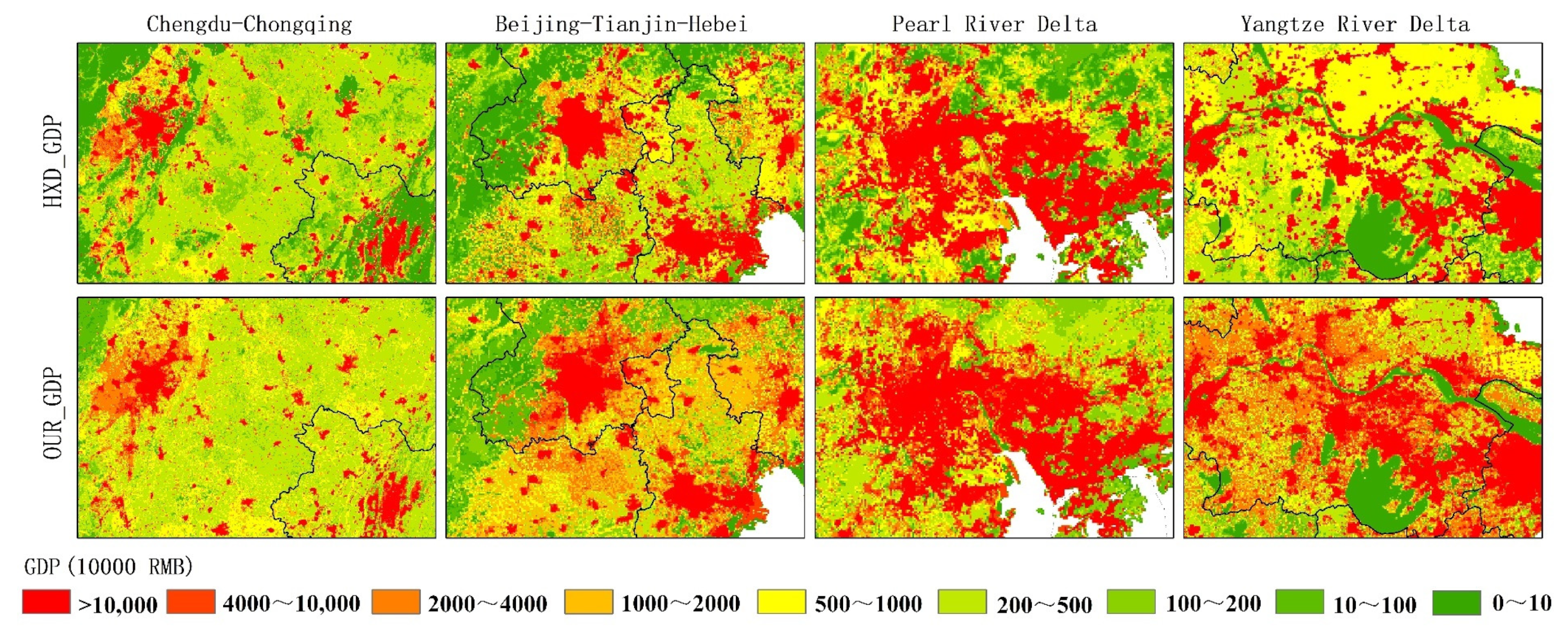
The spatialization results of GDP are highly accurate and can precisely depict the internal differences within county-level administrative units. Using more refined scale town-level GDP statistical data to evaluate the accuracy of the GDP spatialization results, the findings indicate that it performs exceptionally well on the town-level validation dataset. Specifically, the R² value reaches 0.78, demonstrating its reliable predictive capability. Additionally, the MAE and RMSE are relatively small. Therefore, the gridded total GDP derived from using the XGBoost model for GDP1 and GDP2, and the RF model for GDP3, exhibits good accuracy. Furthermore, when compared to publicly available GDP datasets, the two show consistent spatial distribution patterns and aggregation trends. Our GDP dataset provides a finer depiction of differences within county-level administrative units.

(3)

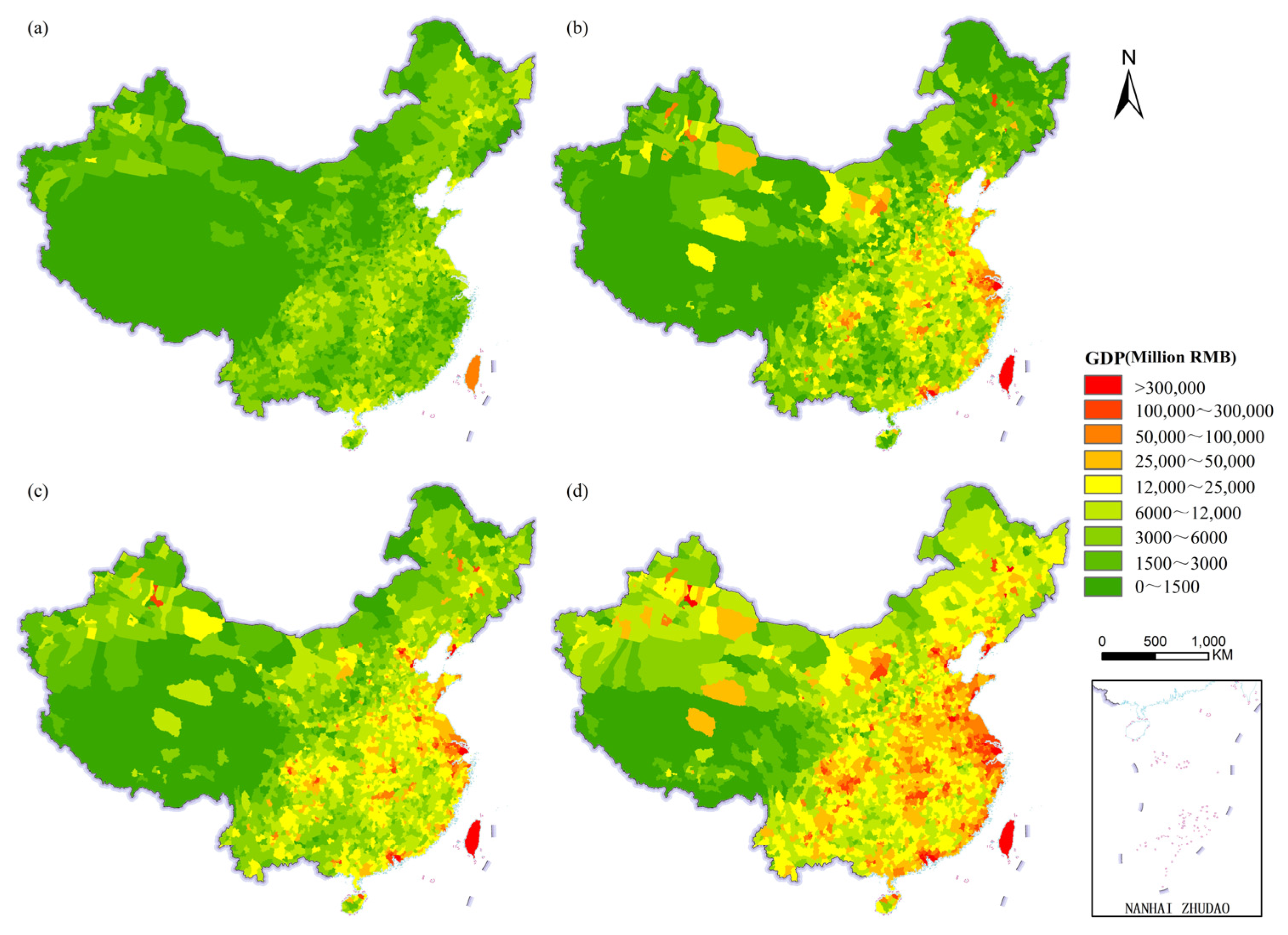
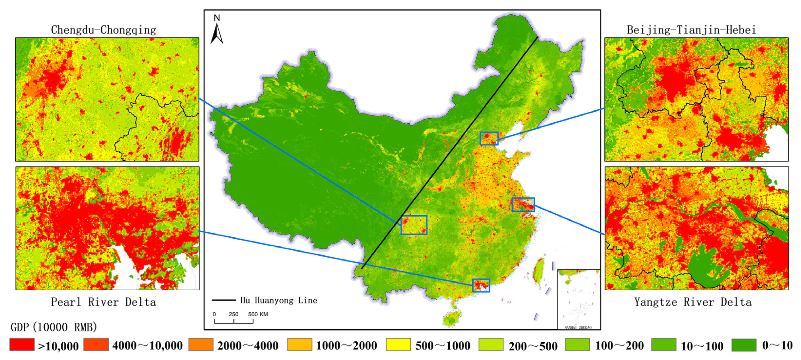
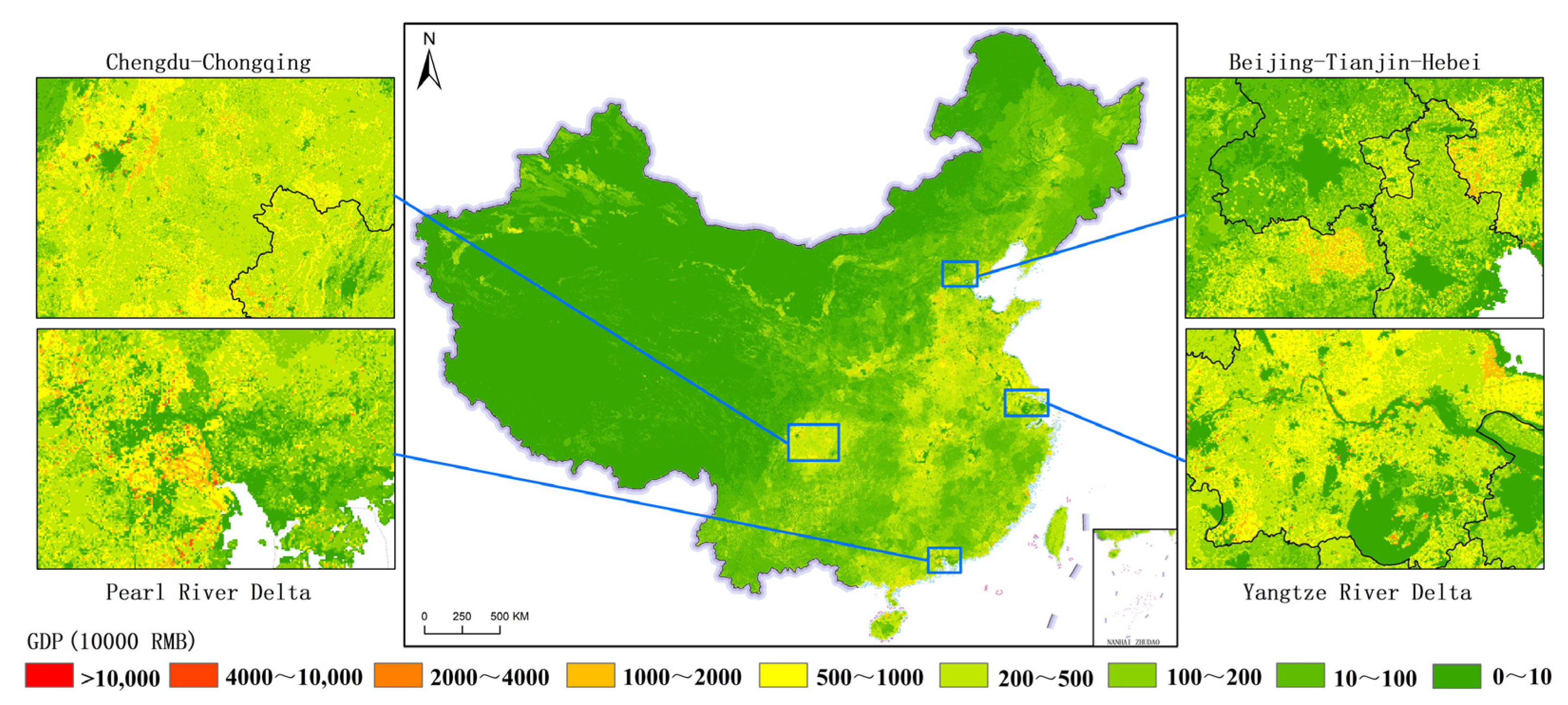
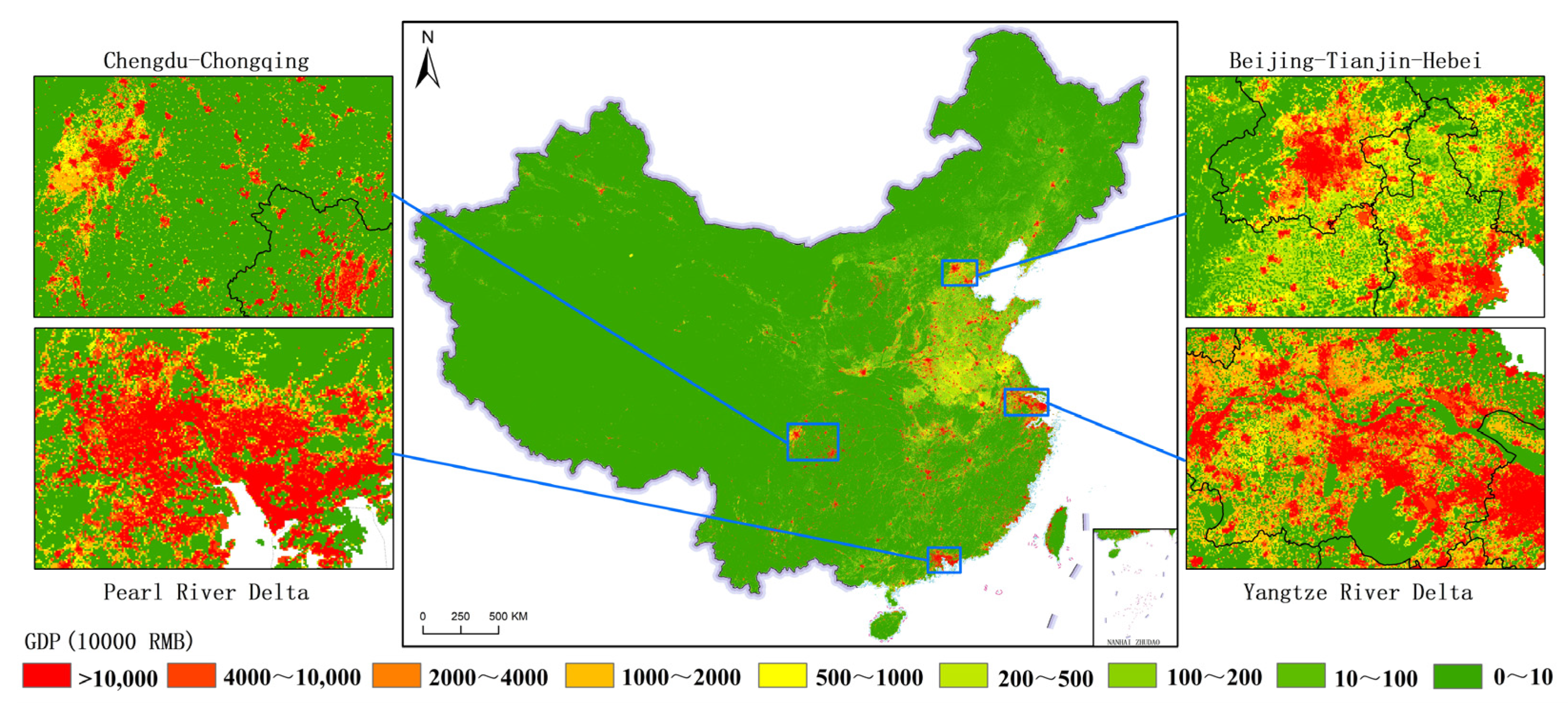
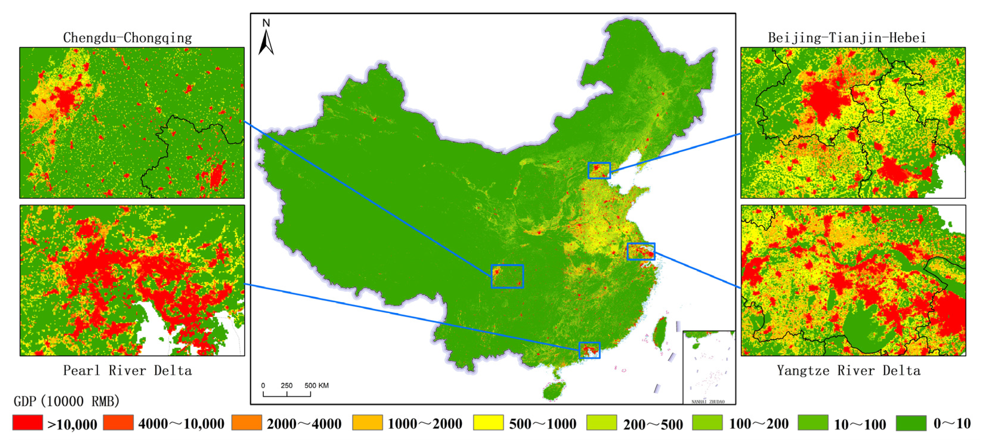
The spatial distribution differences in the three major industries are remarkable. On the whole, China’s GDP is divided by the “Hu Huanyong line”. The relatively high GDP is mainly distributed in the Huang–Huai–Hai Plain and the eastern coastal areas on the southeast side of the line, while the relatively low GDP is mainly distributed in most areas of Tibet, Qinghai, Xinjiang, and inner Mongolia on the northwest side of the line. Overall, the number of high-value GDP grids ranks as follows: tertiary industry > secondary industry > primary industry. Regarding the distribution of high-value GDP grids, primary industry is mainly located in suburban and rural areas. The secondary and tertiary industries are primarily distributed in large cities and their surroundings, with the former being more prevalent in suburban areas and the latter being more concentrated in city centers. The spatial distribution differences among the gridded GDP for the three industries are consistent with the actual distribution of real GDP.

References

1. Geiger, T. Continuous National Gross Domestic Product (GDP) Time Series for 195 Countries: Past Observations (1850–2005) Harmonized with Future Projections According to the Shared Socio-Economic Pathways (2006–2100). Earth Syst. Sci. Data 2018, 10, 847–856. [Google Scholar] [CrossRef]
2. Henderson, J.V.; Storeygard, A.; Weil, D.N. Measuring Economic Growth from Outer Space. Am. Econ. Rev. 2012, 102, 994–1028. [Google Scholar] [CrossRef] [PubMed]
3. Sutton, P.C.; Costanza, R. Global Estimates of Market and Non-Market Values Derived from Nighttime Satellite Imagery, Land Cover, and Ecosystem Service Valuation. Ecol. Econ. 2002, 41, 509–527. [Google Scholar] [CrossRef]
4. Chen, X.; Nordhaus, W.D. Using Luminosity Data as a Proxy for Economic Statistics. Proc. Natl. Acad. Sci. USA 2011, 108, 8589–8594. [Google Scholar] [CrossRef]
5. Wang, W.; Cheng, H.; Zhang, L. Poverty Assessment Using DMSP/OLS Night-Time Light Satellite Imagery at a Provincial Scale in China. Adv. Space Res. 2012, 49, 1253–1264. [Google Scholar] [CrossRef]
6. Gu, H.; Chen, C.; Lu, Y.; Chu, Y.; Ma, Y. Construction of Regional Economic Development Model Based on Remote Sensing Data. IOP Conf. Ser. Earth Environ. Sci. 2019, 310, 052060. [Google Scholar] [CrossRef]
7. Huang, Z.; Li, S.; Gao, F.; Wang, F.; Lin, J.; Tan, Z. Evaluating the Performance of LBSM Data to Estimate the Gross Domestic Product of China at Multiple Scales: A Comparison with NPP-VIIRS Nighttime Light Data. J. Clean. Prod. 2021, 328, 129558. [Google Scholar] [CrossRef]
8. Liao, F.H.F.; Wei, Y.D. Dynamics, Space, and Regional Inequality in Provincial China: A Case Study of Guangdong Province. Appl. Geogr. 2012, 35, 71–83. [Google Scholar] [CrossRef]
9. Chen, J.; Li, L. Regional Economic Activity Derived From MODIS Data: A Comparison With DMSP/OLS and NPP/VIIRS Nighttime Light Data. IEEE J. Sel. Top. Appl. Earth Obs. Remote Sens. 2019, 12, 3067–3077. [Google Scholar] [CrossRef]
10. Chen, Y.; Wu, G.; Ge, Y.; Xu, Z. Mapping Gridded Gross Domestic Product Distribution of China Using Deep Learning with Multiple Geospatial Big Data. Ieee J. Stars 2022, 15, 1791–1802. [Google Scholar] [CrossRef]
11. Kummu, M.; Taka, M.; Guillaume, J.H.A. Gridded Global Datasets for Gross Domestic Product and Human Development Index over 1990–2015. Sci. Data 2018, 5, 180004. [Google Scholar] [CrossRef] [PubMed]
12. Yue, T.; Zhao, N.; Liu, Y.; Wang, Y.; Zhang, B.; Du, Z.; Fan, Z.; Shi, W.; Chen, C.; Zhao, M.; et al. A fundamental theorem for eco-environmental surface modelling and its applications. Sci. China (Earth Sci.) 2020, 63, 1092–1112. [Google Scholar] [CrossRef]
13. Ye, T.; Zhao, N.; Yang, X.; Ouyang, Z.; Liu, X.; Chen, Q.; Hu, K.; Yue, W.; Qi, J.; Li, Z.; et al. Improved Population Mapping for China Using Remotely Sensed and Points-of-Interest Data within a Random Forests Model. Sci. Total Environ. 2019, 658, 936–946. [Google Scholar] [CrossRef]
14. Elvidge, C.D.; Baugh, K.E.; Kihn, E.A.; Kroehl, H.W.; Davis, E.R.; Davis, C.W. Relation between Satellite Observed Visible-near Infrared Emissions, Population, Economic Activity and Electric Power Consumption. Int. J. Remote Sens. 1997, 18, 1373–1379. [Google Scholar] [CrossRef]
15. Zhao, N.; Liu, Y.; Cao, G.; Samson, E.L.; Zhang, J. Forecasting China’s GDP at the Pixel Level Using Nighttime Lights Time Series and Population Images. GIScience Remote Sens. 2017, 54, 407–425. [Google Scholar] [CrossRef]
16. Guo, B.; Hu, D.; Wang, S.; Lin, A.; Kuang, H. Estimation of Gridded Anthropogenic Heat Flux at the Optimal Scale by Integrating SDGSAT-1 Nighttime Lights and Geospatial Data. Int. J. Appl. Earth Obs. Geoinf. 2023, 125, 103596. [Google Scholar] [CrossRef]
17. Li, X.; Xu, H.; Chen, X.; Li, C. Potential of NPP-VIIRS Nighttime Light Imagery for Modeling the Regional Economy of China. Remote Sens. 2013, 5, 3057–3081. [Google Scholar] [CrossRef]
18. Guo, B.; Hu, D.; Zheng, Q. Potentiality of SDGSAT-1 Glimmer Imagery to Investigate the Spatial Variability in Nighttime Lights. Int. J. Appl. Earth Obs. Geoinf. 2023, 119, 103313. [Google Scholar] [CrossRef]
19. Liu, S.; Liu, W.; Zhou, Y.; Wang, S.; Wang, Z.; Wang, Z.; Wang, Y.; Wang, X.; Hao, L.; Wang, F. Analysis of Economic Vitality and Development Equilibrium of China’s Three Major Urban Agglomerations Based on Nighttime Light Data. Remote Sens. 2024, 16, 4571. [Google Scholar] [CrossRef]
20. Liu, S.; Zhou, Y.; Wang, F.; Wang, S.; Wang, Z.; Wang, Y.; Qin, G.; Wang, P.; Liu, M.; Huang, L. Lighting Characteristics of Public Space in Urban Functional Areas Based on SDGSAT-1 Glimmer Imagery:A Case Study in Beijing, China. Remote Sens. Environ. 2024, 306, 114137. [Google Scholar] [CrossRef]
21. Deng, F.; Cao, L.; Li, F.; Li, L.; Man, W.; Chen, Y.; Liu, W.; Peng, C. Mapping China’s Changing Gross Domestic Product Distribution Using Remotely Sensed and Point-of-Interest Data with Geographical Random Forest Model. Sustainability 2023, 15, 8062. [Google Scholar] [CrossRef]
22. Chen, Q.; Hou, X.; Zhang, X.; Ma, C. Improved GDP Spatialization Approach by Combining Land-Use Data and Night-Time Light Data: A Case Study in China’s Continental Coastal Area. Int. J. Remote Sens. 2016, 37, 4610–4622. [Google Scholar] [CrossRef]
23. Liang, H.; Guo, Z.; Wu, J.; Chen, Z. GDP Spatialization in Ningbo City Based on NPP/VIIRS Night-Time Light and Auxiliary Data Using Random Forest Regression. Adv. Space Res. 2020, 65, 481–493. [Google Scholar] [CrossRef]
24. Zhao, M.; Cheng, W.; Zhou, C.; Li, M.; Wang, N.; Liu, Q. GDP Spatialization and Economic Differences in South China Based on NPP-VIIRS Nighttime Light Imagery. Remote Sens. 2017, 9, 673. [Google Scholar] [CrossRef]
25. Chen, T.; Zhou, Y.; Zou, D.; Wu, J.; Chen, Y.; Wu, J.; Wang, J. Deciphering China’s Socio-Economic Disparities: A Comprehensive Study Using Nighttime Light Data. Remote Sens. 2023, 15, 4581. [Google Scholar] [CrossRef]
26. Li, F.; Mao, L.; Chen, Q.; Yang, X. Refined Estimation of Potential GDP Exposure in Low-Elevation Coastal Zones (LECZ) of China Based on Multi-Source Data and Random Forest. Remote Sens. 2023, 15, 1285. [Google Scholar] [CrossRef]
27. Xu, Z.; Wang, Y.; Sun, G.; Chen, Y.; Ma, Q.; Zhang, X. Generating Gridded Gross Domestic Product Data for China Using Geographically Weighted Ensemble Learning. ISPRS Int. J. Geo-Inf. 2023, 12, 123. [Google Scholar] [CrossRef]
28. Wu, N.; Yan, J.; Liang, D.; Sun, Z.; Ranjan, R.; Li, J. High-Resolution Mapping of GDP Using Multi-Scale Feature Fusion by Integrating Remote Sensing and POI Data. Int. J. Appl. Earth Obs. Geoinf. 2024, 129, 103812. [Google Scholar] [CrossRef]
29. Chen, Z.; Wang, W.; Zong, H.; Yu, X. Precise GDP Spatialization and Analysis in Built-Up Area by Combining the NPP-VIIRS-like Dataset and Sentinel-2 Images. Sensors 2024, 24, 3405. [Google Scholar] [CrossRef]
30. Ustaoglu, E.; Bovkır, R.; Aydınoglu, A.C. Spatial Distribution of GDP Based on Integrated NPS-VIIRS Nighttime Light and MODIS EVI Data: A Case Study of Turkey. Environ. Dev. Sustain. 2021, 23, 10309–10343. [Google Scholar] [CrossRef]
31. Li, W.; Wu, M.; Niu, Z. Spatialization and Analysis of China’s GDP Based on NPP/VIIRS Data from 2013 to 2023. Appl. Sci. 2024, 14, 8599. [Google Scholar] [CrossRef]
32. Murakami, D.; Yamagata, Y. Estimation of Gridded Population and GDP Scenarios with Spatially Explicit Statistical Downscaling. Sustainability 2019, 11, 2106. [Google Scholar] [CrossRef]
33. Zhang, H.; Dong, G.; Li, B.; Xie, Z.; Miao, C.; Yang, F.; Gao, Y.; Meng, X.; Yang, D.; Liu, Y.; et al. Developing an Annual Global Sub-National Scale Economic Data from 1992 to 2021 Using Nighttime Lights and Deep Learning. Int. J. Appl. Earth Obs. Geoinf. 2024, 133, 104086. [Google Scholar] [CrossRef]
34. Chen, Z.; Yu, B.; Yang, C.; Zhou, Y.; Yao, S.; Qian, X.; Wang, C.; Wu, B.; Wu, J. An Extended Time Series (2000–2018) of Global NPP-VIIRS-like Nighttime Light Data from a Cross-Sensor Calibration. Earth Syst. Sci. Data 2021, 13, 889–906. [Google Scholar] [CrossRef]
35. Stevens, F.R.; Gaughan, A.E.; Linard, C.; Tatem, A.J. Disaggregating Census Data for Population Mapping Using Random Forests with Remotely-Sensed and Ancillary Data. PLoS ONE 2015, 10, e0107042. [Google Scholar] [CrossRef]
36. Lundberg, S.M.; Lee, S.-I. A Unified Approach to Interpreting Model Predictions. In Proceedings of the 31st International Conference on Neural Information Processing Systems, Long Beach, CA, USA, 4–9 December 2017; Curran Associates Inc.: Red Hook, NY, USA, 2017; pp. 4768–4777. [Google Scholar]
37. Han, X.; Zhou, Y.; Wang, S.; Wang, L.; Hou, Y. Spatialization Approach to 1 km Grid GDP Based on Remote Sensing. In Proceedings of the 2011 International Conference on Multimedia Technology, Hangzhou, China, 26–28 July 2011; pp. 739–742. [Google Scholar]
38. Doll, C.N.H.; Muller, J.-P.; Morley, J.G. Mapping Regional Economic Activity from Night-Time Light Satellite Imagery. Ecol. Econ. 2006, 57, 75–92. [Google Scholar] [CrossRef]
39. Wang, K.; Ji, X.; Liu, S.; Zhu, J.; Liu, K. Harnessing Big Data for Sustainable Urban Management: A Novel Approach to Gridded Urban GDP Dataset Development. J. Clean. Prod. 2024, 444, 141205. [Google Scholar] [CrossRef]
40. Zhou, Y.; Ma, T.; Zhou, C.; Xu, T. Nighttime Light Derived Assessment of Regional Inequality of Socioeconomic Development in China. Remote Sens. 2015, 7, 1242–1262. [Google Scholar] [CrossRef]
Figure 1. Study area. (Note: Based on the standard map of the Ministry of Natural Resources standard map service website with the approval number GS (2023) 2763, the base map boundary is not modified. The same after).
Remotesensing 17 01709 g001
Figure 2. Land use and NTL data in 2020.
Remotesensing 17 01709 g002
Figure 3. China’s county-level GDP statistical data in 2020 ((a) primary industry; (b) second industry; (c) tertiary industry; (d) Total GDP).
Remotesensing 17 01709 g003
Figure 4. Schematic diagram of the modeling processes of FAM and GAM.
Remotesensing 17 01709 g004
Figure 5. Results of feature importance analysis: (a) From the XGBoost model of the primary industry; (b) From the XGBoost model of the secondary industry; (c) From the RF model of the tertiary industry.
Remotesensing 17 01709 g005
Figure 6. China’s 1 km gridded GDP in 2020.
Remotesensing 17 01709 g006
Figure 7. China’s 1 km gridded GDP1 in 2020.
Remotesensing 17 01709 g007
Figure 8. China’s 1 km gridded GDP2 product in 2020.
Remotesensing 17 01709 g008
Figure 9. China’s 1 km gridded GDP3 product in 2020.
Remotesensing 17 01709 g009
Figure 10. China’s 1 km gridded Xu_GDP dataset in 2020.
Remotesensing 17 01709 g010
Figure 11. China’s 1 km gridded HXD_GDP dataset in 2020.
Remotesensing 17 01709 g011
Figure 12. Comparison between HXD_GDP dataset and OUR_GDP dataset.
Remotesensing 17 01709 g012