

Classification of Forest Stratification and Evaluation of Forest Stratification Changes over Two Periods Using UAV-LiDAR

Abstract
1. Introduction
2. Materials and Methods
2.1. Study Area
2.2. LiDAR Measurements
2.3. Data Analysis
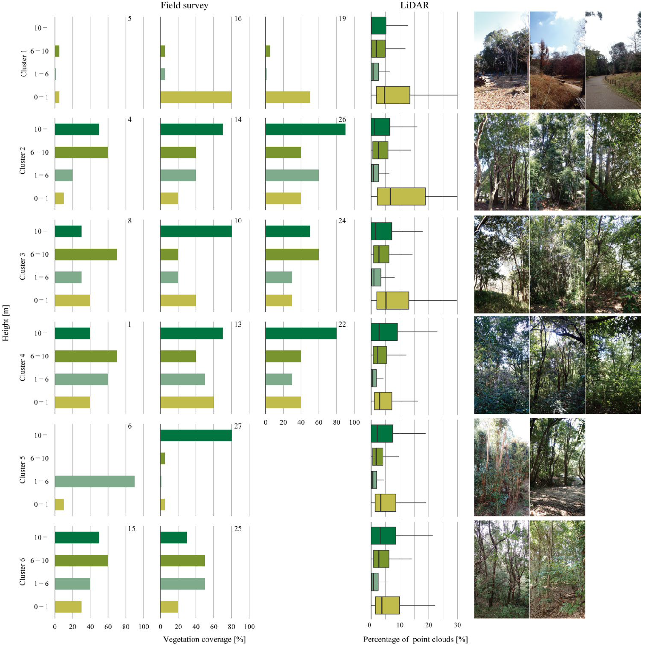
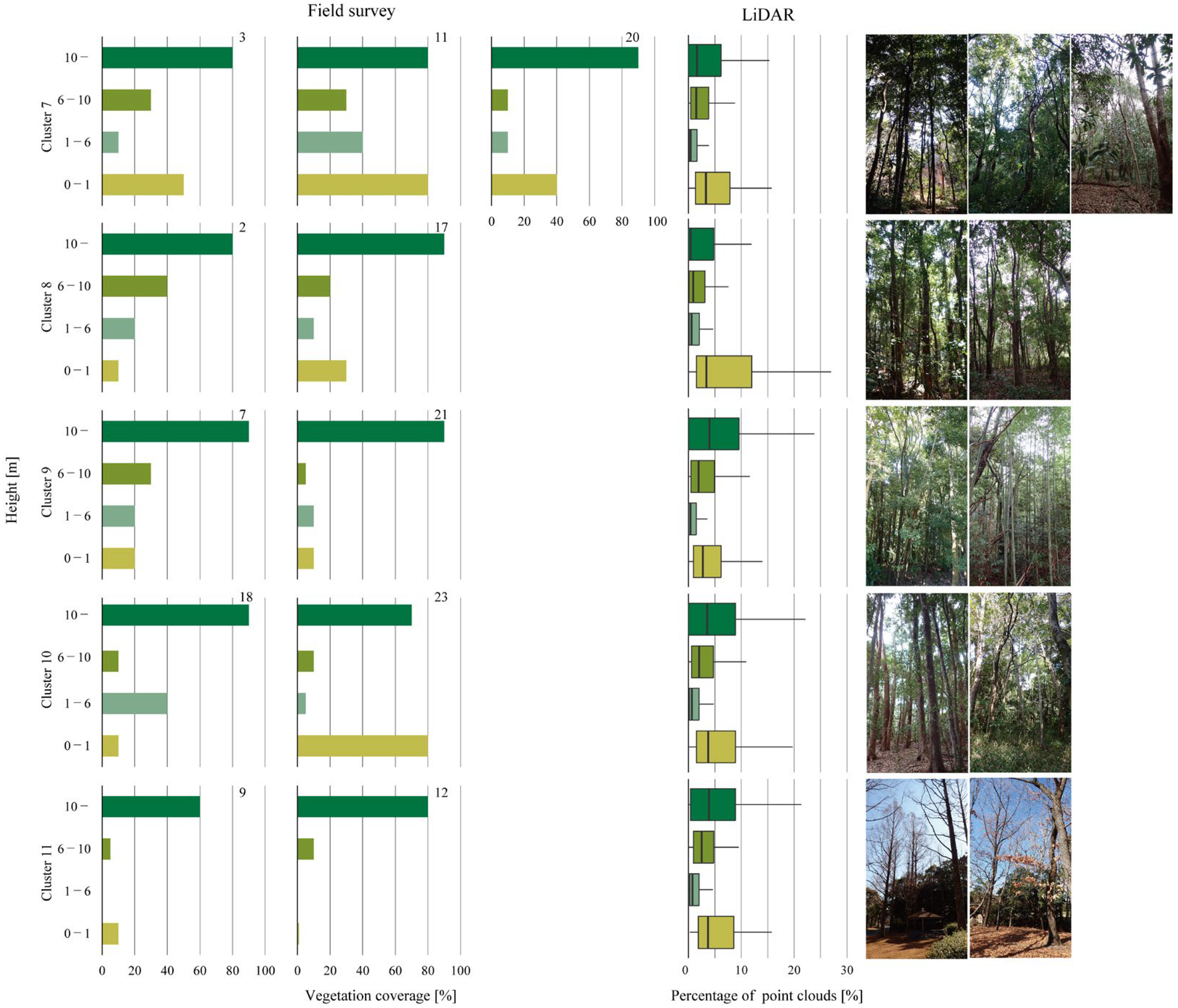
2.4. Verification
3. Results
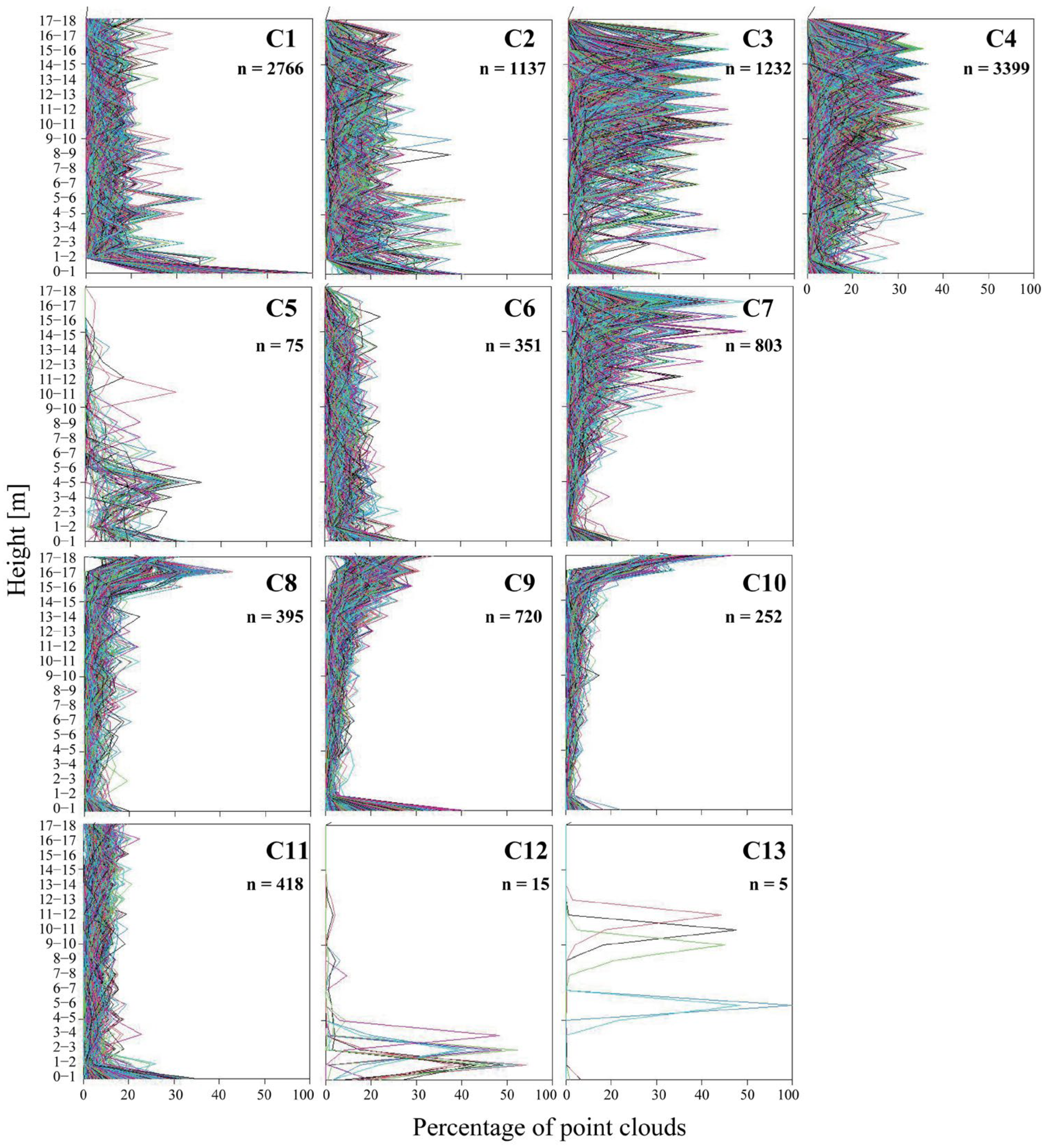
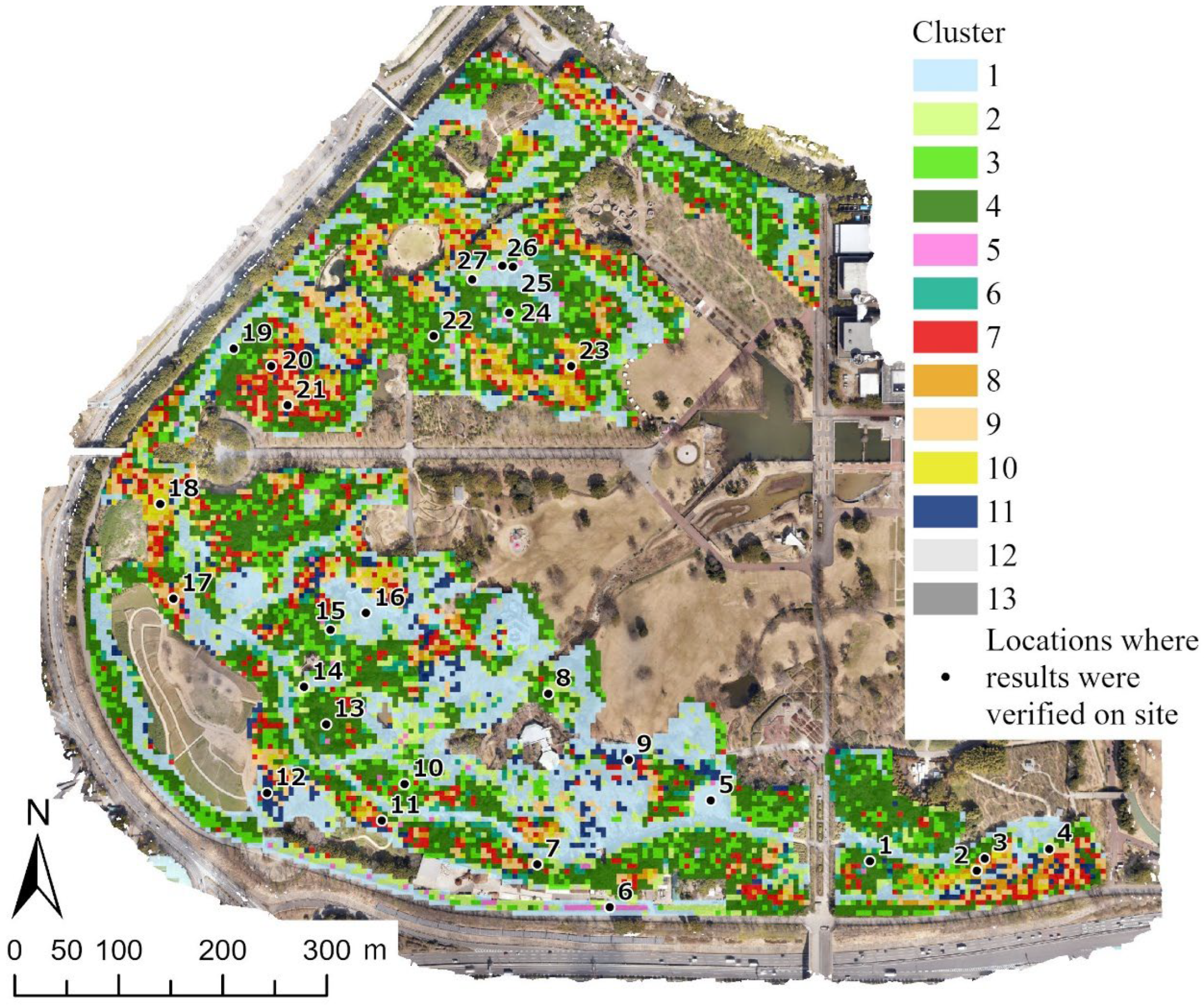
3.1. Classification of Forest Stratification
3.2. Changes in Forest Stratification
4. Discussion
4.1. Classification of Forest Stratification
4.2. Changes in Forest Stratification
4.3. Potential Applications of Proposed Method
5. Conclusions
Funding
Data Availability Statement
Acknowledgments
Conflicts of Interest
References
- Coops, N.C.; Tompalski, P.; Goodbody, T.R.H.; Queinnec, M.; Luther, J.E.; Bolton, D.K.; White, J.C.; Wulder, M.A.; van Lier, O.R.; Hermosilla, T. Modelling lidar-derived estimates of forest attributes over space and time: A review of approaches and future trends. Remote Sens. Environ. 2021, 260, 112477. [Google Scholar] [CrossRef]
- Beland, M.; Parker, G.; Sparrow, B.; Harding, D.; Chasmer, L.; Phinn, S.; Antonarakis, A.; Strahler, A. On promoting the use of lidar systems in forest ecosystem research. For. Ecol. Manag. 2019, 450, 117484. [Google Scholar] [CrossRef]
- Neuville, R.; Bates, J.S.; Jonard, F. Estimating forest structure from UAV-mounted LiDAR point cloud using machine learning. Remote Sens. 2021, 13, 352. [Google Scholar] [CrossRef]
- Lim, K.; Treitz, P.; Wulder, M.; St-Onge, B.; Flood, M. LiDAR remote sensing of forest structure. Prog. Phys. Geogr. Earth Environ. 2003, 27, 88–106. [Google Scholar] [CrossRef]
- Guo, Q.; Su, Y.; Hu, T.; Zhao, X.; Wu, F.; Li, Y.; Liu, J.; Chen, L.; Xu, G.; Lin, G.; et al. An integrated UAV-borne lidar system for 3D habitat mapping in three forest ecosystems across China. Int. J. Remote Sens. 2017, 38, 2954–2972. [Google Scholar] [CrossRef]
- Dubayah, R.O.; Drake, J.B. Lidar Remote Sensing for Forestry. Remote Sens. 2000, 98, 44–46. [Google Scholar]
- Hamraz, H.; Contreras, M.A.; Zhang, J. Vertical stratification of forest canopy for segmentation of understory trees within small-footprint airborne LiDAR point clouds. ISPRS J. Photogramm. Remote Sens. 2017, 130, 385–392. [Google Scholar] [CrossRef]
- Jiang, X.; Li, G.; Lu, D.; Chen, E.; Wei, X. Stratification-based forest aboveground biomass estimation in a subtropical region using airborne lidar data. Remote Sens. 2020, 12, 1101. [Google Scholar] [CrossRef]
- Yun, Z.; Zheng, G.; Geng, Q.; Monika Moskal, L.; Wu, B.; Gong, P. Dynamic stratification for vertical forest structure using aerial laser scanning over multiple spatial scales. Int. J. Appl. Earth Obs. Geoinf. 2022, 114, 103040. [Google Scholar] [CrossRef]
- Means, J.E.; Acker, S.A.; Harding, D.J.; Blair, B.; Lefsky, M.A.; Cohen, W.B.; Harmon, M.E.; Mckee, W.A. Use of Large-Footprint Scanning Airborne Lidar To Estimate Forest Stand Characteristics in the Western Cascades of Oregon. Remote Sens. Environ. 1999, 67, 298–308. [Google Scholar] [CrossRef]
- Domiciano Galvincio, J.; Popescu, S.C. Measuring Individual Tree Height and Crown Diameter for Mangrove Trees with Airborne Lidar Data. Int. J. Adv. Eng. Manag. Sci. 2016, 2, 239456. [Google Scholar]
- Agca, M.; Popescu, S.C.; Harper, C.W. Deriving forest canopy fuel parameters for loblolly pine forests in eastern Texas. Can. J. For. Res. 2011, 41, 1618–1625. [Google Scholar] [CrossRef]
- Zimble, D.A.; Evans, D.L.; Carlson, G.C.; Parker, R.C.; Grado, S.C.; Gerard, P.D. Characterizing vertical forest structure using small-footprint airborne LiDAR. Remote Sens Env. 2003, 87, 171–182. [Google Scholar] [CrossRef]
- Kellner, J.R.; Armston, J.; Birrer, M.; Cushman, K.C.; Duncanson, L.; Eck, C.; Falleger, C.; Imbach, B.; Král, K.; Krůček, M.; et al. New Opportunities for Forest Remote Sensing Through Ultra-High-Density Drone Lidar. Surv. Geophys. 2019, 40, 959–977. [Google Scholar] [CrossRef]
- Ma, K.; Chen, Z.; Fu, L.; Tian, W.; Jiang, F.; Yi, J.; Du, Z.; Sun, H. Performance and Sensitivity of Individual Tree Segmentation Methods for UAV-LiDAR in Multiple Forest Types. Remote Sens. 2022, 14, 298. [Google Scholar] [CrossRef]
- Liu, L.; Pang, Y.; Li, Z.; Si, L.; Liao, S. Combining airborne and terrestrial laser scanning technologies to measure forest understorey volume. Forests 2017, 8, 111. [Google Scholar] [CrossRef]
- Jacon, A.D.; Galvão, L.S.; Martins-Neto, R.P.; Crespo-Peremarch, P.; Aragão, L.E.O.C.; Ometto, J.P.; Anderson, L.O.; Vedovato, L.B.; Silva-Junior, C.H.L.; Lopes, A.P.; et al. Characterizing Canopy Structure Variability in Amazonian Secondary Successions with Full-Waveform Airborne LiDAR. Remote Sens. 2024, 16, 2085. [Google Scholar] [CrossRef]
- Singh, A.; Kushwaha, S.K.P. Forest Degradation Assessment Using UAV Optical Photogrammetry and SAR Data. J. Indian Soc. Remote Sens. 2021, 49, 559–567. [Google Scholar] [CrossRef]
- Gong, Y.; Xie, H.; Liao, S.; Lu, Y.; Jin, Y.; Wei, C.; Tong, X. Assessing the Accuracy of Multi-Temporal GlobeLand30 Products in China Using a Spatiotemporal Stratified Sampling Method. Remote Sens. 2023, 15, 4593. [Google Scholar] [CrossRef]
- Yu, J.W.; Yoon, Y.W.; Baek, W.K.; Jung, H.S. Forest vertical structure mapping using two-seasonal optic images and lidar dsm acquired from uav platform through random forest, xgboost, and support vector machine approaches. Remote Sens 2021, 13, 4282. [Google Scholar] [CrossRef]
- Montero, P.; Vilar, J.A. TSclust: An R package for time series clustering. J. Stat. Softw. 2014, 62, 1–43. [Google Scholar] [CrossRef]
- Lovell, J.L.; Jupp, D.L.B.; Culvenor, D.S.; Coops, N.C. Using airborne and ground-based ranging lidar to measure canopy structure in Australian forests. Can. J. Remote Sens. 2003, 29, 607–622. [Google Scholar] [CrossRef]
- van Leeuwen, M.; Nieuwenhuis, M. Retrieval of forest structural parameters using LiDAR remote sensing. Eur. J. For. Res. 2010, 129, 749–770. [Google Scholar] [CrossRef]
- Coops, N.C.; Hilker, T.; Wulder, M.A.; St-Onge, B.; Newnham, G.; Siggins, A.; Trofymow, J.A. Estimating canopy structure of Douglas-fir forest stands from discrete-return LiDAR. Trees-Struct. Funct. 2007, 21, 295–310. [Google Scholar] [CrossRef]
- Jain, A.K.; Murty, M.N.; Flynn, P.J. Data clustering: A review. ACM Comput. Surv. 1999, 31, 264–323. [Google Scholar] [CrossRef]
- Dronova, I.; Kislik, C.; Dinh, Z.; Kelly, M. A Review of Unoccupied Aerial Vehicle Use in Wetland Applications: Emerging Opportunities in Approach, Technology, and Data. Drones 2021, 5, 45. [Google Scholar] [CrossRef]


| 2022 | 2024 | |||||
|---|---|---|---|---|---|---|
| Height [m] | Total Number of Points | Average Value of Ratio of the Number of Points | SD of Ratio of the Number of Points | Total Number of Points | Average Value of Ratio of the Number of Points | SD of Ratio of the Number of Points |
| 0–1 | 19,638,505 | 21.4 | 27.5 | 56,405,386 | 23.5 | 28.6 |
| 1–2 | 1,549,171 | 1.7 | 4.4 | 4,069,204 | 1.6 | 4.3 |
| 2–3 | 1,730,906 | 1.8 | 3.9 | 4,782,441 | 1.8 | 3.9 |
| 3–4 | 1,994,324 | 2.1 | 3.8 | 5,590,471 | 2.1 | 4.0 |
| 4–5 | 2,475,637 | 2.4 | 3.9 | 7,202,450 | 2.5 | 4.8 |
| 5–6 | 2,871,546 | 2.8 | 4.1 | 7,059,462 | 2.6 | 4.2 |
| 6–7 | 3,399,157 | 3.3 | 4.7 | 7,870,296 | 3.0 | 4.4 |
| 7–8 | 4,222,814 | 3.9 | 5.1 | 9,252,247 | 3.5 | 4.7 |
| 8–9 | 5,284,427 | 4.7 | 5.8 | 11,297,075 | 4.3 | 5.5 |
| 9–10 | 6,342,703 | 5.5 | 6.9 | 13,618,852 | 5.1 | 6.4 |
| 10–11 | 6,799,118 | 6.0 | 7.6 | 15,287,256 | 5.6 | 7.0 |
| 11–12 | 6,897,893 | 6.3 | 7.4 | 16,223,810 | 6.1 | 7.2 |
| 12–13 | 7,738,343 | 7.2 | 8.9 | 17,823,650 | 6.8 | 8.2 |
| 13–14 | 8,514,329 | 8.0 | 10.4 | 19,725,588 | 7.5 | 9.4 |
| 14–15 | 8,150,082 | 7.8 | 10.9 | 20,724,559 | 7.8 | 10.6 |
| 15–16 | 6,660,758 | 6.5 | 10.6 | 18,535,793 | 7.0 | 10.6 |
| 16–17 | 4,651,100 | 4.8 | 9.5 | 13,779,564 | 5.4 | 10.0 |
| 17–18 | 3,045,343 | 3.6 | 9.7 | 8,633,966 | 3.9 | 9.8 |
Disclaimer/Publisher’s Note: The statements, opinions and data contained in all publications are solely those of the individual author(s) and contributor(s) and not of MDPI and/or the editor(s). MDPI and/or the editor(s) disclaim responsibility for any injury to people or property resulting from any ideas, methods, instructions or products referred to in the content. |
© 2025 by the author. Licensee MDPI, Basel, Switzerland. This article is an open access article distributed under the terms and conditions of the Creative Commons Attribution (CC BY) license (https://creativecommons.org/licenses/by/4.0/).
Share and Cite
Niwa, H. Classification of Forest Stratification and Evaluation of Forest Stratification Changes over Two Periods Using UAV-LiDAR. Remote Sens. 2025, 17, 1682. https://doi.org/10.3390/rs17101682
Niwa H. Classification of Forest Stratification and Evaluation of Forest Stratification Changes over Two Periods Using UAV-LiDAR. Remote Sensing. 2025; 17(10):1682. https://doi.org/10.3390/rs17101682
Chicago/Turabian StyleNiwa, Hideyuki. 2025. "Classification of Forest Stratification and Evaluation of Forest Stratification Changes over Two Periods Using UAV-LiDAR" Remote Sensing 17, no. 10: 1682. https://doi.org/10.3390/rs17101682
APA StyleNiwa, H. (2025). Classification of Forest Stratification and Evaluation of Forest Stratification Changes over Two Periods Using UAV-LiDAR. Remote Sensing, 17(10), 1682. https://doi.org/10.3390/rs17101682