Quantifying the Impact of Vegetation Greening on Evapotranspiration and Its Components on the Tibetan Plateau

Abstract

The Tibetan Plateau (TP) serves as a vital ecological safeguard and water conservation region in China. In recent decades, substantial efforts have been made to promote vegetation greening across the TP; however, these interventions have added complexity to the local water balance and evapotranspiration (ET) processes. To investigate these dynamics, we apply the Priestley–Taylor Jet Propulsion Laboratory (PT-JPL) model to simulate ET components in the TP. Through model sensitivity experiments, we isolate the contribution of vegetation greening to ET variations. Furthermore, we analyze the role of climatic drivers on ET using a suite of statistical techniques. Based on satellite and climate data from 1982 to 2018, we found the following: (1) The PT-JPL model successfully captured ET trends over the TP, revealing increasing trends in total ET, canopy transpiration, interception loss, and soil evaporation at rates of 0.06, 0.39, 0.005, and 0.07 mm/year, respectively. The model’s performance was validated using eddy covariance observations from three flux tower sites, yielding R² values of 0.81–0.86 and RMSEs ranging from 6.31 to 13.20 mm/month. (2) Vegetation greening exerted a significant enhancement on ET, with the mean annual ET under greening scenarios (258.6 ± 120.9 mm) being 2.9% greater than under non-greening scenarios (251.2 ± 157.2 mm) during 1982–2018. (3) Temperature and vapor pressure deficit were the dominant controls on ET, influencing 53.5% and 23% of the region, respectively, as identified consistently by both multiple linear regression and dominant factor analyses. These findings highlight the net influence of vegetation greening and offer valuable guidance for water management and sustainable ecological restoration efforts in the region.

1. Introduction

Evapotranspiration (ET) is crucial for Earth’s ecosystems, hydrological processes, and biogeochemical cycles [1]. It represents the total water vapor flux from land surfaces and vegetation to the atmosphere [2]. Globally, terrestrial ET accounts for approximately 60% of precipitation returning to the atmosphere, making it a significant contributor to the terrestrial water cycle, second only to precipitation itself [3]. It also plays a critical role in the global energy and water cycles [4]. In this study, ET is divided into three main components: vegetation canopy transpiration (ETc), soil evaporation (ETs), and intercepted evapotranspiration (ETi). ET mainly comprises evaporation from soil and water surfaces, evaporation of precipitation or dew intercepted by vegetation canopies, vegetation transpiration, and snow sublimation [5,6]. Compared to ETs and ETi, ETc constitutes the largest proportion of ET in terrestrial ecosystems [7,8]. As highlighted in prior studies [9], ET dynamics are shaped by both climatic variability and terrestrial vegetation conditions. Shifts in climate influence ET primarily through alterations in atmospheric water vapor capacity and indirect effects on plant physiological activity [10]. Additionally, fluctuations in regional soil moisture—resulting from climate anomalies—can further modulate ET responses. Vegetation, on the other hand, impacts ET by intercepting precipitation, modifying land surface roughness, and affecting hydrological pathways such as runoff generation [11]. These vegetation–ET interactions have co-evolved over time, leading to a dynamic balance in the ecohydrological system. Large-scale ecological restoration efforts, particularly those focused on vegetation enhancement, bring about improvements in local ecological quality while simultaneously transforming surface energy and water exchange characteristics [12]. However, the extent and direction of vegetation greening’s impact on ET are highly dependent on spatial and temporal context. For example, in the Loess Plateau, vegetation improvements have been found to exert stronger control over ET than climate forcing [13], whereas in northern China, ET variability appears to be more sensitive to changes in precipitation regimes [14]. Consequently, disentangling and quantifying the individual and combined contributions of vegetation changes and climate variability to ET patterns is essential for informed water resource governance and sustainable land use planning [15]. Recent global-scale analyses further confirm that vegetation greening significantly modulates ET trends by enhancing canopy transpiration and altering surface energy balance, although the magnitude and direction of this influence vary across climatic zones and vegetation types [16].

Accurate quantification of ET necessitates the use of reliable data sources, and several methodologies are available to obtain such data, including in situ observations and satellite-based approaches [17]. While ground-based techniques—such as lysimeters, eddy covariance systems, and the Bowen ratio method—are capable of delivering high-precision ET measurements, their application is constrained by limited spatial and temporal coverage, whereas remote sensing technologies help overcome these limitations by enabling large-scale monitoring of surface parameters essential for ET estimation [18]. In contrast, remote sensing technologies overcome these limitations by enabling large-scale monitoring of surface parameters essential for ET estimation. For example, Landsat 8 OLI imagery has been integrated with the METRIC model to assess ET and evaluate surface energy fluxes under present-day climate conditions [19]. This approach has revealed notable spatial differences in ET across varying land cover categories. As a result, calibration of model parameters tailored to specific land use types becomes essential for improving ET estimation accuracy [20]. In a more recent application, both METRIC and the Two-Source Energy Balance (TSEB) models have been employed, using eddy covariance data as validation references, to estimate ET and energy fluxes in floodplain environments located at the junction of the Morava and Taya Rivers in the Czech Republic [21]. Scholars have shown that although the two models are generally consistent with EC observations, differences still exist in the spatial distribution of ET, possibly due to variations in surface temperature retrieval or parameterization schemes [19]. Therefore, there is still much room for improvement in remote sensing-based energy balance models for capturing the spatial heterogeneity of hydrological fluxes.

In the study of hydrological spatial distribution, ET data from satellite sensors are insufficient to fully clarify the physical interaction between ET and other hydrological variables, or to predict future spatial and temporal changes in ET [22]. To overcome these challenges, various hydrological models have been developed to estimate ET, including the Priestley–Taylor Jet Propulsion Laboratory (PT-JPL) model [23]. Originating from the Priestley–Taylor (PT) framework, the PT-JPL model estimates ET as a portion of potential ET and has proven effective for simulating regional ecosystem water fluxes [24]. By incorporating vegetation characteristics and meteorological inputs, the model applies a set of biophysical constraints to accurately replicate ET patterns and the associated land–atmosphere water exchange processes in a given area [25]. Notably, the PT-JPL model requires minimal ground-based observations, making it well suited for large-scale applications and future ET projections. When integrated with satellite remote sensing, this modeling approach enables ET estimation across both regional and global domains [26]. As a result, ET simulation models have gained widespread adoption and have been extensively implemented in diverse geographical settings [27].

The TP, the world’s highest and largest plateau, is characterized by distinctive geographic and climatic conditions and plays a crucial role in the global climate system [28]. However, the grassland ecosystem of the TP is highly sensitive, fragile, and vulnerable to damage. Once damaged, it is exceedingly difficult to restore. These ecological problems not only affect the local ecosystem and residents’ lives, but also have a profound impact on the downstream ecology [29]. Over recent decades, China has implemented a series of large-scale ecological restoration efforts on the TP, including programs like “grazing exclusion for grassland recovery” and “wetland conservation” [30]. These initiatives have brought about significant shifts in vegetation cover across the region. While they have contributed to mitigating soil erosion, concerns have emerged regarding their potential to intensify water resource depletion and further aggravate regional water scarcity issues [31]. In the process of returning farmland to forests, some areas did not follow the principle of balance between vegetation greening and water resources supply and demand, breaking the original vegetation-water resources dynamic equilibrium relationship; excessive vegetation greening led to a large amount of soil and water resources were consumed, and then a new ecological problem appeared, represented by soil desiccation and degradation of vegetation [32,33]. Recent research suggests that, under ongoing global warming, extensive ecological restoration and vegetation enhancement may exert increasingly complex influences on ET dynamics across the TP [34].

Due to the limitation of climate and other conditions on the TP, there are still some studies on the quantitative relationship between vegetation greening and water consumption on the TP focused on the point scale [35]. The strong spatial and temporal variability in vegetation water consumption patterns makes point-scale observations and analyses inadequate for providing a theoretical foundation for a vegetation greening strategy across the entire TP [36]. As a result, current efforts are even less equipped to support strategies aimed at optimizing water resource utilization [6]. At the regional level, long-term investigations into how vegetation protection and greening influence water use and related transformation processes remain insufficient. Moreover, the complex interactions between vegetation dynamics, climate variability, and the hydrological cycle have yet to be fully elucidated, and the dominant controls on ET processes over the TP are still not clearly identified. This underscores the urgent need for a systematic evaluation of how vegetation changes and climate fluctuations affect regional ET and its components—namely canopy transpiration (ETc), interception loss (ETi), and soil evaporation (ETs). Such an assessment will contribute important knowledge to guide regional water resource management and vegetation restoration strategies, while also informing the design of future ecological policies.

In this study, we applied the PT-JPL model to investigate spatial and temporal patterns of ET across the TP from 1982 to 2018, considering two distinct scenarios: one incorporating vegetation change and the other assuming static vegetation conditions. The primary aim is to assess how shifts in vegetation influence regional ET by addressing the following research objectives: (1) evaluating the net impact of vegetation change on ET and its components; (2) analyzing the intricate interplay between climate change and vegetation greening on ET, pinpointing the dominant factors in different areas, and offering guidance for water resource management, vegetation conservation, and ecological strategies.

2. Materials and Methods

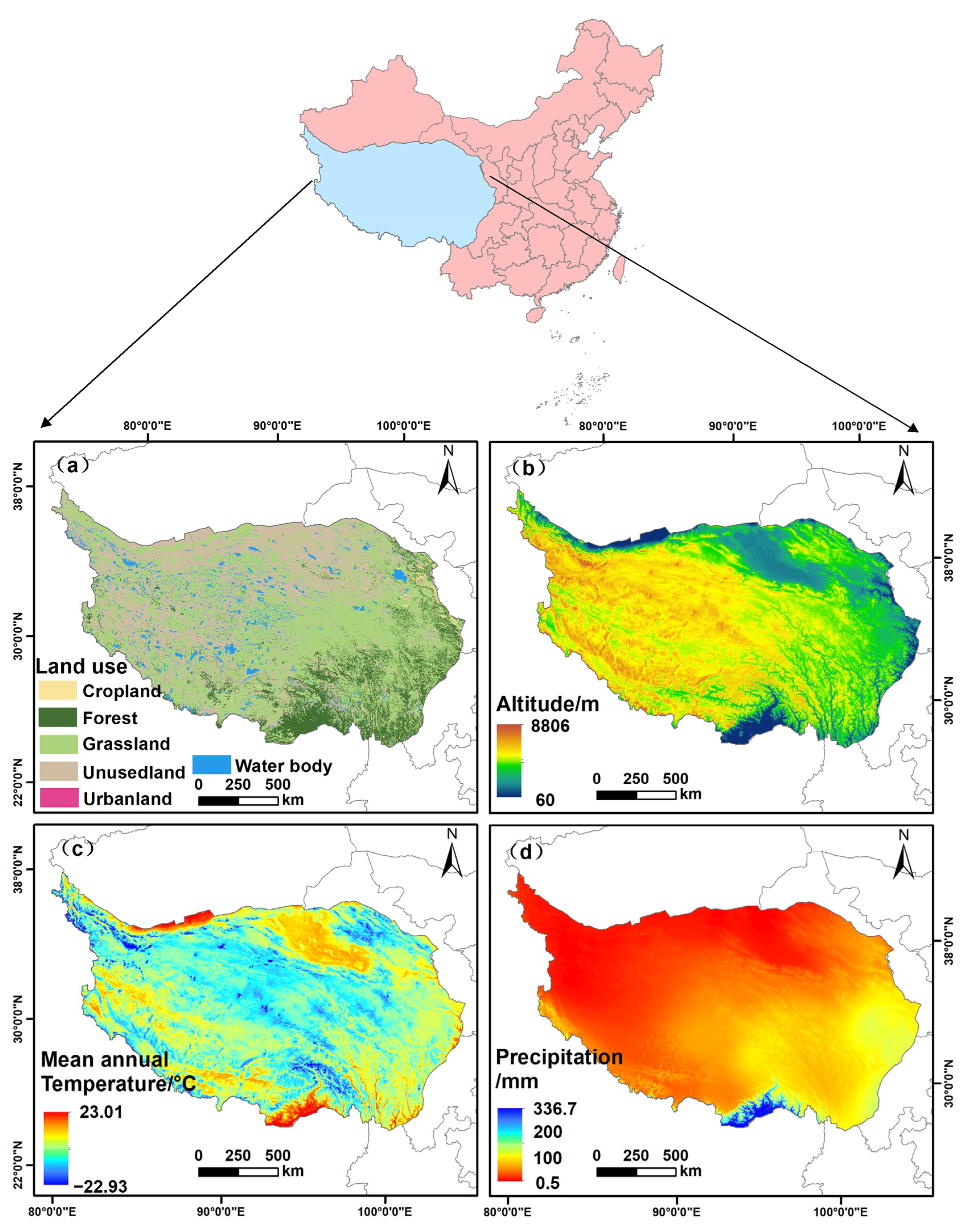
2.1. Overview of the Study Area

Located in southwestern China, the TP is renowned as the “Roof of the World” due to its exceptional elevation. Extending from 73°19′E to 104°47′E and 26°00′N to 39°47′N (Figure 1a), the TP has an average elevation exceeding 4000 m, making it the highest plateau on Earth [37]. The ecological environment is unique and fragile, comprising diverse ecosystems such as alpine meadows, grasslands, wetlands, lakes, and glaciers. Grasslands dominate the landscape, covering nearly 60% of the region (Figure 1b) [38]. The dominant soil types include subalpine meadow soils, alpine meadow soils, and subalpine grassland soils [39]. The plateau’s rugged topography forms high-altitude canyons, steep waterfalls, and deeply incised gorges, leading to rapid river flows and high water potential [40]. The climate is complex and strongly influenced by altitude and terrain. Figure 1c shows the distribution of annual average temperature, which reveals strong altitudinal gradients, with extremely cold winters and relatively mild summers. In addition, the TP experiences large diurnal temperature variation and intense solar radiation. Annual precipitation is less than 100 mm in parts of the northwestern TP, as highlighted by the color bar marker in Figure 1d. Most rainfall occurs in summer, while winters are typically dry [41].

2.2. Data Sources

Meteorological data were sourced from the China Meteorological Forcing Dataset (CMFD) [42,43,44], available at https://data.tpdc.ac.cn/zh-hans/data/8028b944-daaa-4511-8769-965612652c49/ (accessed on 1 June 2024). This dataset provides multiple atmospheric variables, including precipitation rate (PRE), surface air temperature (TEM, °C), water vapor pressure (hPa), and near-surface air pressure (Pa) [33,45]. It offers a temporal resolution of 3 h and a spatial resolution of 0.1°, covering the period from 1979 to 2018. For this study, we used data from 1982 to 2018.

Albedo data with a spatial resolution of 0.05° were obtained from the GLASS product (https://glass-product.bnu.edu.cn/ (accessed on 10 June 2024)). Specifically, we used GLASS02B05 for the period 1982–1999 and GLASS02B06 for 2000–2018.

Vapor Pressure Deficit (VPD, kPa) data at 0.5° resolution were obtained from the CRU TS v4.06 dataset (https://crudata.uea.ac.uk/ (accessed on 6 June 2024)), which spans from 1901 to 2023. In this study, we selected the period 1982–2018 for consistency with other data inputs [33].

The absorbed radiation dose (RAD), expressed in rad, is calculated using the following equation [6]:

$$R_{nshort}=(1-p)I_t$$

(1)

$$R_{nlong}=R_{ld}-R_{lu}$$

(2)

$$R_{lu}=\sigma T^4$$

(3)

In these formulas, $p$ denotes the surface albedo, $I_t$ refers to the incoming shortwave radiation, $R_{ld}$ and $R_{lu}$ represent the downward and upward longwave radiation, respectively. The symbol $\sigma$ stands for the Stefan–Boltzmann constant, with a value of 5.67 × 10⁻⁸ W·m⁻²·K⁻⁴. T corresponds to temperature measured in Kelvin (K) [46].

$$R_n=R_{nshort}-R_{nlong}$$

(4)

In this expression, $R_n$ denotes the net radiation, while $R_{nshort}$ and $R_{nlong}$ represent the net shortwave and net longwave radiation components, respectively [32].

$$R_{ns}=\left(R_{n}exp\right(-k_{R_n}LAI\left)\right)$$

(5)

$$R_{nc}=R_n-R_{ns}$$

(6)

Within this equation, $R_{ns}$ represents the fraction of net radiation transmitted to the soil surface, whereas $R_{nc}$ corresponds to the component absorbed by the canopy. The extinction coefficient, symbolized as $k_{R_n}$, is set to a constant value of 0.6 [32,45]. All radiation variables discussed here are quantified in watts per square meter (W·m⁻²).

For vegetation information, the Normalized Difference Vegetation Index (NDVI) was obtained from the GIMMS dataset (https://daac.ornl.gov/VEGETATION/guides/Global_Veg_Greenness_GIMMS_3G.html (accessed on 15 March 2024)). Monthly NDVI estimates were produced using 14–16 day compositing periods, derived from corrected and calibrated data acquired by the Advanced Very High Resolution Radiometer (AVHRR), AVHRR data were acquired from [NOAA/EUMETSAT], generated by the Advanced Very High Resolution Radiometer (AVHRR/3) manufactured by ITT Exelis (now L3Harris Technologies) in Rochester, NY, USA. This dataset provides global coverage from 1982 to 2022, with a spatial resolution of 0.0833° [45,47]. In this study, multiple vegetation variables were used to characterize vegetation dynamics and their influence on ET. Specifically, the Normalized Difference Vegetation Index (NDVI), Leaf Area Index (LAI), and Fractional Vegetation Cover (FVC) were included. NDVI and FVC were used to parameterize vegetation greenness and canopy fraction, respectively, while LAI was employed in the radiation and transpiration submodules of the PT-JPL model to modulate canopy conductance and interception evaporation. These variables jointly ensured a comprehensive representation of vegetation effects on ET. LAI and FVC data, with a spatial resolution of 0.05°, were sourced from the GLASS product (https://www.geodata.cn/thematicView/, accessed on 15 March 2024) on an annual basis [48].

Land use and land cover (LULC) data at 1 km resolution were obtained from the National Earth System Science Data Center (https://www.geodata.cn/). To meet the needs of this study, the original LULC classes were reclassified into five broader categories: forest, grassland, cropland, shrubland, and bare land.

To evaluate the accuracy of the model-simulated ET, we used two independent data sources for validation. First, ground-based ET data were obtained from three eddy covariance flux tower sites across the TP: Haibei Shrubland (CN-Ha2, 101.32°E, 37.61°N), Haibei Alpine Meadow (CN-HaM, 101.18°E, 37.37°N), and Dangxiong (CN-Dan, 102.59°E, 32.85°N). These datasets were accessed from the FLUXNET data portal (https://fluxnet.org/sites/site-list-and-pages/) [49]. Each site is equipped with a CSAT3 sonic anemometer (Campbell Scientific, Logan, UT, USA) and an LI-7500 infrared gas analyzer (LI-COR Biosciences, Lincoln, NE, USA), with a sampling frequency of 10 Hz and flux-averaging interval of 30 min. ET was calculated using the water balance method based on GC01 and GC07 soil moisture tables in combination with site-level precipitation observations. Second, we employed the Global Land Evaporation Amsterdam Model (GLEAM) version 3.5a dataset (https://www.gleam.eu) [33] to validate ET estimates at the regional scale. This version incorporates updated meteorological inputs and improved parameterization of evaporation components, making it suitable for long-term climatological assessment. Together, the FLUXNET and GLEAM datasets provided robust observational constraints to evaluate the performance of the PT-JPL model across different spatial scales.

Ultimately, the raster datasets mentioned previously were converted to a 0.25° spatial resolution for further analysis. To maintain the integrity and reliability of our data, stringent quality control and assurance measures were implemented. These measures are crucial for minimizing uncertainties and enhancing the precision of model simulations.

2.3. Research Methods

2.3.1. Evaluation of ET

We adopted the Priestley–Taylor Jet Propulsion Laboratory (PT-JPL) model [20] to simulate vegetation ET over the TP. The model was implemented in a GIS environment, integrating spatial datasets including land cover, albedo, vegetation indices (e.g., LAI, NDVI), radiation, and meteorological variables at the pixel level. Total ET is decomposed into three components:

$$ET={ET}_c+{ET}_s+{ET}_i$$

(7)

where ET_c is canopy transpiration, ET_s is soil evaporation, and ET_i is canopy interception evaporation. The individual fluxes are calculated as follows:

$${ET}_c=(1-f_{wet})f_g{f}_t{f}_m\alpha {\displaystyle \frac{\Delta }{\Delta +\gamma }}{R}_{nc}$$

(8)

$${ET}_s=(1-f_{wet}+f_{sm})(1-f_{wet})\alpha {\displaystyle \frac{\Delta }{\Delta +\gamma }}(R_{ns}-G)$$

(9)

$${ET}_i=f_{wet}\alpha {\displaystyle \frac{\Delta }{\Delta +\gamma }}{R}_{nc}$$

(10)

Here, α = 1.26 is the Priestley–Taylor coefficient, Δ is the slope of the saturation vapor pressure curve, and γ is the psychrometric constant (0.066 kPa·°C⁻¹). R_nc and R_ns are net radiation to the canopy and soil, respectively, and are estimated using an exponential decay function based on LAI.

To support reproducibility, key biophysical constraint variables (e.g., fwet, fg, ft, fm) were derived from remote sensing and meteorological datasets. The calculation details and data sources are summarized in

Table 1. Variables and functions used in the PT-JPL model.

Symbol	Description	Function/Formula	Data Source
$f_{wet}$	Surface wetness fraction	$f_{wet}=R{H}^4$	CMFD RH
$f_g$	Green canopy fraction	$f_g={\displaystyle \frac{f_{APAR}}{f_{IPAR}}}$	MODIS NDVI
$f_t$	Temperature constraint	$f_t=exp(-({\displaystyle \frac{T-T_{opt}}{T_{opt}^2}}{)}^2)$	CMFD Temperature
$f_m$	Moisture constraint	$f_m={\displaystyle \frac{f_{APAR}+1}{f_{APARmax+1}}}$	MODIS LAI
$f_{sm}$	Soil moisture constraint	$f_{sm}=R{H}^{VPD/\beta }$	CMFD RH, VPD
$f_{APAR}$	Fraction of absorbed PAR	$f_{APAR}=b_1\times (1-\exp (-k_1\times LAI\left)\right)$	MODIS LAI
$f_{IPAR}$	Fraction of intercepted PAR	$f_{IPAR}=b_2\times (1-\exp (-k_2\times LAI\left)\right)$	MODIS LAI

.

Model parameters (e.g., k₁, k₂, β) were calibrated by comparing simulated ET with GLEAM-based products and optimized for different land cover types. For instance, in forest areas, k₁ = 0.57, k₂ = 0.81, and β = 1.28, whereas in croplands, k₁ = 0.59, k₂ = 0.84, and β = 1.43. The optimal temperature $T_{opt}$ was set as the long-term growing-season mean surface temperature (1982–2018), derived from CMFD data.

Soil heat flux (G) was estimated as

$$G=R_n\left[{\mathit{\Gamma }}_c+\left(1-M\right)\left({\mathit{\Gamma }}_s-{\mathit{\Gamma }}_c\right)\right]$$

(11)

where Γ_c = 0.05, Γ_s = 0.325, and M is monthly vegetation coverage.

2.3.2. Metrics for Verifying PT-JPL Model Outcomes

To validate the performance of the PT-JPL model, we used three evaluation metrics: bias, root mean square error (RMSE), and the Pearson correlation coefficient (R). These indicators were calculated by comparing model-simulated ET values with ground-based observations and GLEAM estimates. Some flux tower observations were excluded from the monthly validation due to sensor malfunction, non-closure of the energy budget, or data quality control criteria (e.g., friction velocity threshold filtering during low-turbulence conditions). These exclusions slightly reduced the total number of valid monthly data points used in the evaluation.

The bias measures the average deviation between simulated and observed values and is calculated as

$$Bias={\displaystyle \frac{1}{n}}{\sum }_{i=1}^n (\mathit{Sim\_i}-\mathit{Obs\_i})$$

(12)

where $\mathit{Sim\_i}$ and $\mathit{Obs\_i}$ denote the simulated and observed ET values, respectively, and n is the number of matched data pairs. A negative bias indicates systematic underestimation, while a positive bias indicates overestimation.

The RMSE quantifies the overall error magnitude and is defined as

$$RMSE=\sqrt{{\displaystyle \frac{1}{n}}{\sum }_{i=1}^n {[\mathit{Sim\_i}-\mathit{Obs\_i}]}^2}$$

(13)

The Pearson correlation coefficient (R) assesses the strength of the linear relationship between simulated and observed values:

$$R={\displaystyle \frac{\sum (\mathit{Obs\_i}-\stackrel{\mathrm{―}}{\mathrm{O}\mathrm{b}\mathrm{s}})(\mathit{Sim\_i}-\stackrel{\mathrm{―}}{\mathrm{S}\mathrm{i}\mathrm{m}})}{\sqrt{\sum (\mathit{Obs\_i}-\stackrel{\mathrm{―}}{\mathrm{O}\mathrm{b}\mathrm{s}}{)}^2\sum (\mathit{Sim\_i}-\stackrel{\mathrm{―}}{\mathrm{S}\mathrm{i}\mathrm{m}}{)}^2}}}$$

(14)

A higher R value indicates a stronger agreement in temporal variation between the two datasets. All calculations follow standard practices in model validation [26,50,51,52].

2.3.3. Control Design of Vegetation Restoration in ET Assessment

To investigate the influence of vegetation dynamics on ET, the PT-JPL model was employed to simulate ET under two contrasting vegetation scenarios: one reflecting temporal changes in vegetation cover, and the other assuming static vegetation conditions. These simulations accounted for major land cover types, including forest, grassland, cropland, and shrubland.

The dynamic vegetation scenario captures ET evolution under natural progression and anthropogenic influences, while the static scenario assumes that vegetation cover remained unchanged throughout the study period. Specifically, for the static case, vegetation conditions in the study area were fixed at their 1982 levels, excluding the impacts of environmental change, climate variation, and ecological restoration policies implemented since that year.

By comparing ET estimates between the dynamic and static vegetation scenarios—i.e., subtracting the latter from the former—the net effect of vegetation change on ET in the TP from 1982 to 2018 was quantified.

2.3.4. Attribution Analysis

We examined the spatial and temporal dynamics of total ET and its three components—canopy transpiration (ET_c), interception evaporation (ET_i), and soil evaporation (ET_s)—alongside their primary environmental drivers: vegetation characteristics and climatic conditions, over the period 1982–2018. To detect significant trends in these variables, we applied the non-parametric Sen–Mann–Kendall test due to its robustness in environmental time series analysis [53].

After identifying trends, all variables—including ET, ET_c, ET_i, ET_s, precipitation (PRE), temperature (TMP), radiation (RAD), vapor pressure deficit (VPD), and LAI—were normalized to ensure comparability across datasets with differing units and magnitudes. The normalization formula is as follows:

$$X_i={\displaystyle \frac{x_i-x_{min}}{x_{max}-x_{min}}}$$

(15)

Subsequently, multiple linear regression (MLR) was performed to quantify the influence of different climatic and vegetation drivers on ET and its components. The regression model is given by

$$Y_{ET}=b_0+b_1{X}_1+b_2{X}_2+\dots +b_i{X}_i+\mu$$

(16)

In this equation, $Y_{ET}$ represents the normalized and detrended ET, $b_0$ is the intercept term, and μ is the error term. $X_i$ is the normalized predictor variables, and $b_i$ denotes their corresponding standardized regression coefficients. Separate MLR models were constructed for ET, ET_c, ET_i, ET_s to evaluate their respective driving factors [54].

To further determine the contribution of each driver to the long-term trend in ET [55], we used the following attribution equation:

$$W_{b{a}_i}={\displaystyle \frac{b_i{X}_{i\_trend}}{Y_{E{T}_{a\_trend}}}}{Y}_{E{T}_{n\_trend}}$$

(17)

Here, $W_{b{a}_i}$ denotes the contribution of driver i to the ET trend. $X_{i\_trend}$, $Y_{E{T}_{a\_trend}}$, and $Y_{E{T}_{n\_trend}}$ represent the temporal trends of the driver, actual ET, and normalized ET, respectively. All trend values are expressed in mm/year.

To identify the dominant driver in each grid cell, we adopted the method proposed by [56], where the variable with the largest positive contribution (among PRE, TMP, RAD, and VPD) is considered dominant if ET exhibits an increasing trend. Conversely, in areas of decreasing ET, the factor with the most negative contribution is classified as dominant [57]. To link the regression-based attribution analysis with spatial interpretation, we computed the contribution weight $W_{b{a}_i}$ for each driving variable at every pixel. These weights quantify the influence of each predictor’s trend on the ET trend, incorporating both the sensitivity (regression coefficient) and the magnitude of change (temporal trend) of the driver.

Subsequently, the dominant factor for each pixel was identified as the variable with the largest positive contribution to the increasing trend in ET. In pixels where ET trends were negative, the variable with the most negative contribution was assigned. This pixel-level attribution was applied separately for total ET, ET_c, ET_i, ET_s, producing spatial maps of dominant drivers.

3. Results

3.1. Double Verification of the Model

3.1.1. Validation of Flux Site Data

We recorded the monthly actual values for the three flux sites over the period from 2002 to 2005 and extracted the corresponding ET grid results from the PT-JPL model simulations, matched by the latitude and longitude coordinates of these sites. Subsequently, we used bias and RMSE to assess the accuracy of our simulation results. The monthly ET simulated by the PT-JPL model was evaluated against flux tower observations at three validation sites: Dan (Figure 2a), HaM (Figure 2b), and Ha2 (Figure 2c). The bias values obtained for these sites were 4.51, −0.22, and −9.85 mm/month, respectively. The coefficient of determination (R²) ranged from 0.81 at Dan to 0.86 at Ha2, while the root mean square error (RMSE) varied between 6.31 mm/month and 13.20 mm/month. These validation metrics indicate an acceptable agreement between the model-simulated ET and in situ flux observations, considering the spatial heterogeneity, complex terrain, and sparse flux tower distribution on the TP. The PT-JPL model captured the seasonal patterns and general magnitudes of ET reasonably well, although some bias remains in specific regions.

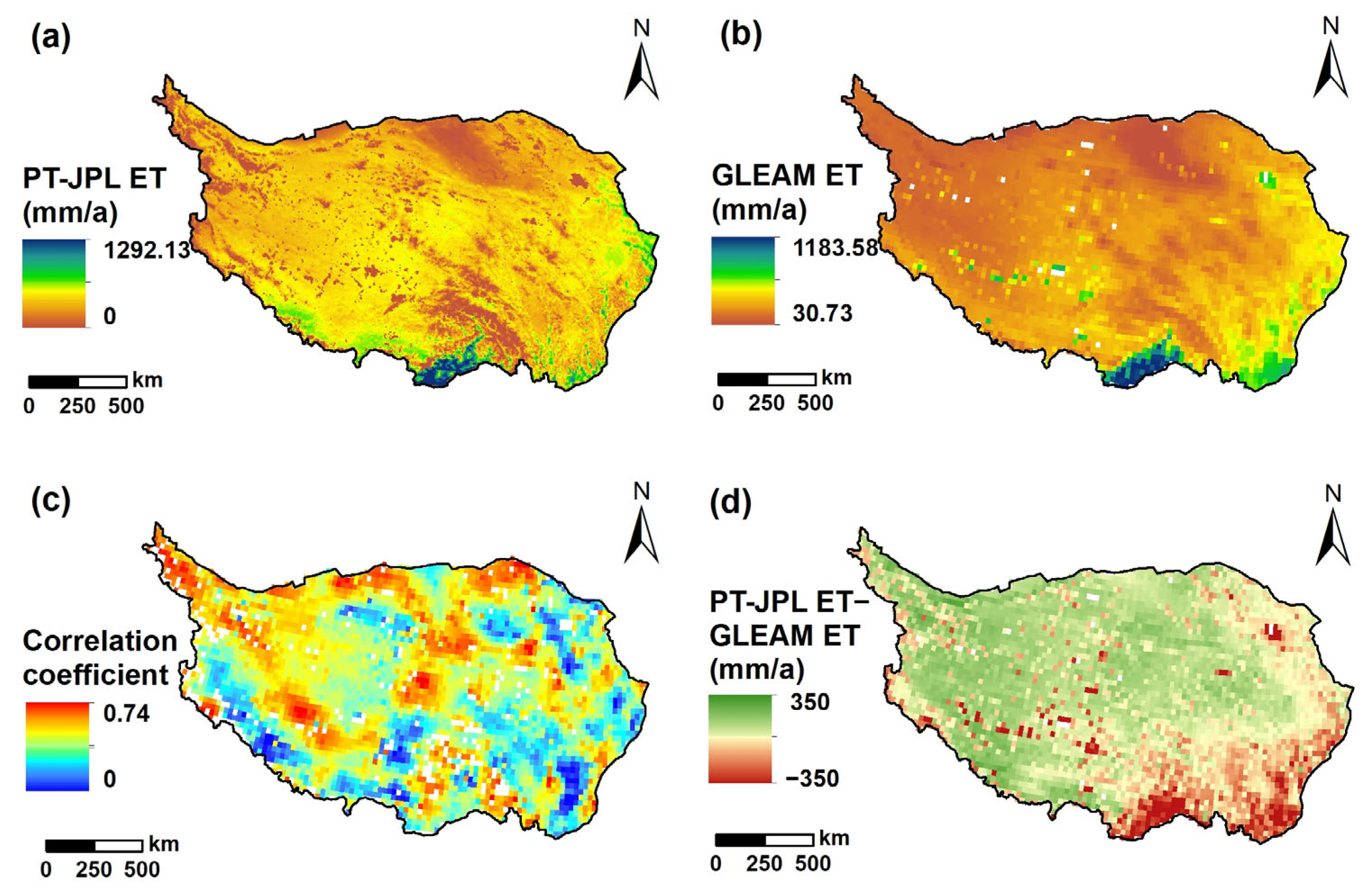
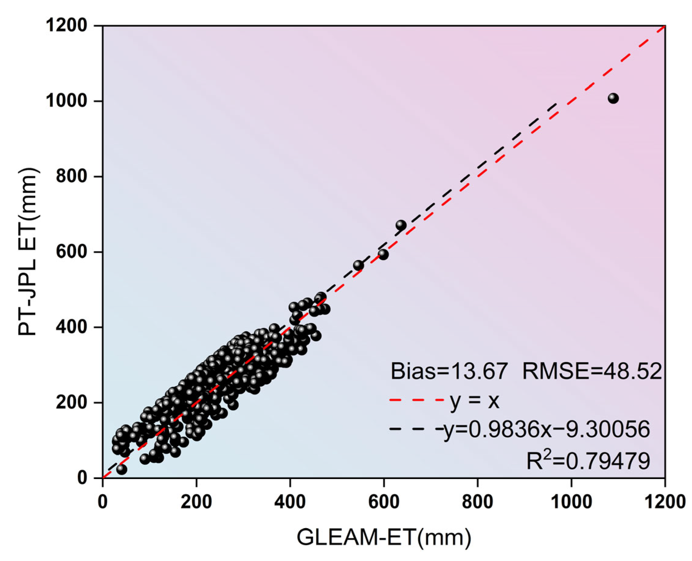
3.1.2. Validation of GLEAM ET

In addition to site-scale validation, we assessed the PT-JPL model’s performance at the regional level using the GLEAM ET dataset across the TP during 1982–2018. As shown in Figure 3, both models exhibit similar spatial patterns of long-term mean ET, with higher values in the southern and western regions of the TP and a north-to-south gradient.

However, notable differences in magnitude and correlation are evident. The spatial correlation coefficient between PT-JPL and GLEAM average ET products exceeds 0.6 in only 8.66% of the TP, and values greater than 0.3 are observed in 69.47% of the plateau, mostly in northern and low-ET regions (Figure 3c). This indicates that agreement varies considerably across land cover types and environmental gradients.

We further compared annual ET outputs from both models, resulting in a coefficient of determination (R²) of 0.79, a bias of 13.67 mm, and a root mean square error (RMSE) of 48.52 mm (Figure 4). While the general trends of ET are broadly consistent, the differences in magnitude and regional response suggest structural differences between the two models. PT-JPL does not account for root-zone soil moisture or complex hydrological memory effects as GLEAM does, which may lead to underestimation or spatial discrepancies in certain regions. These limitations are further discussed in Section 4.

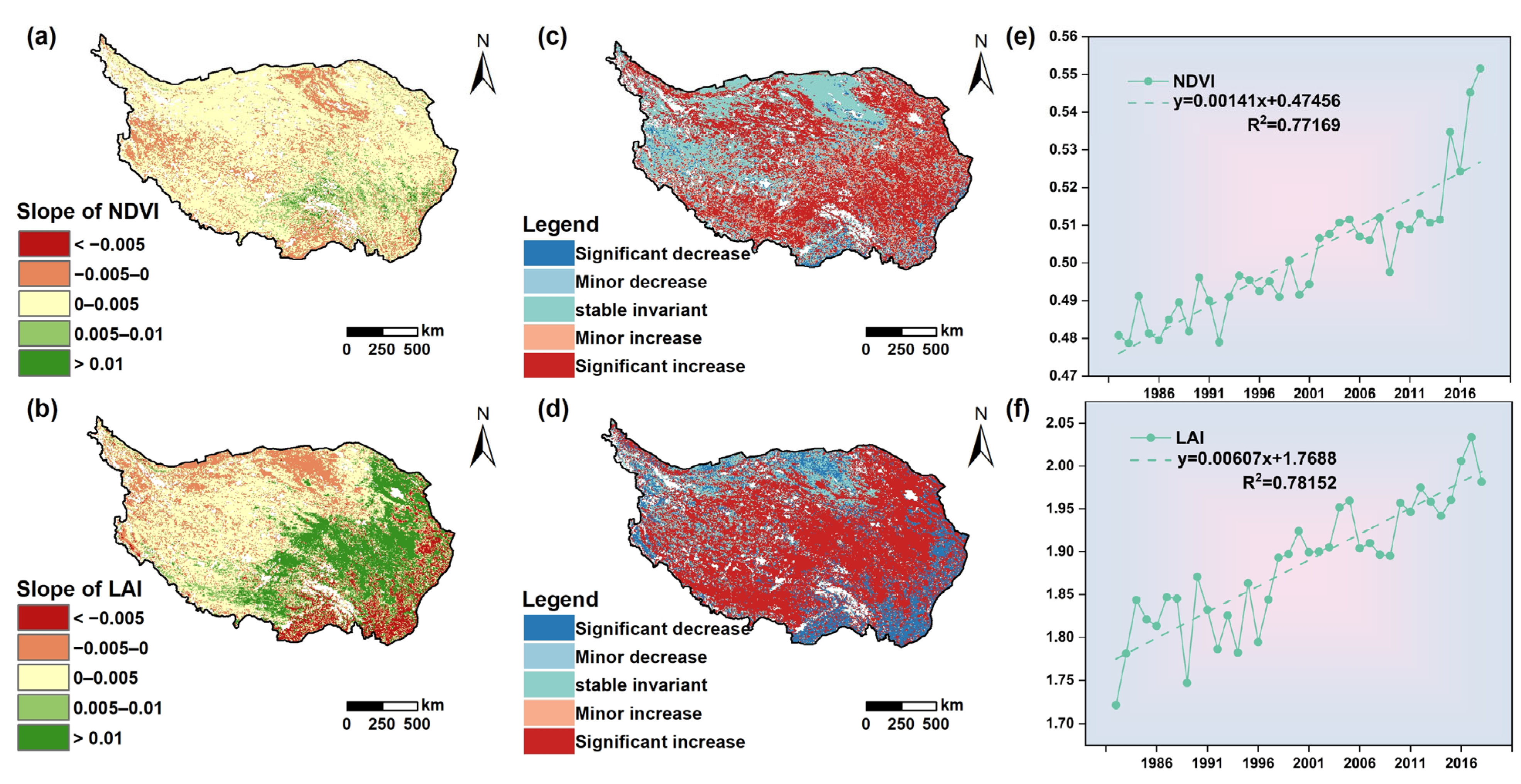
3.2. Spatiotemporal Dynamics of Vegetation Evolution

Statistically significant (p < 0.05) spatiotemporal trends in NDVI and LAI across the TP were identified for the period 1982–2018. As illustrated in Figure 5a, NDVI exhibited considerable spatial heterogeneity, revealing distinct biogeographical patterns across the plateau. These trends reflect the combined influence of climatic variability, ecological restoration, and land cover dynamics over recent decades. Approximately 72% of the plateau demonstrated positive vegetation growth patterns (Sen’s slope > 0), particularly in east–central grasslands (e.g., southern Qinghai and the source regions of the Yellow and Yangtze Rivers), where large-scale ecological restoration programs have been implemented. Contrastingly, 18% of northern and southeastern regions exhibited vegetation degradation (Sen’s slope < 0), primarily in ecologically vulnerable zones with sparse vegetation cover (<0.3 NDVI baseline). Climatological analysis indicates that stable NDVI/LAI values (|Sen’s slope| ≤ 0.001/yr) predominantly occurred in xeric grasslands (mean annual precipitation < 300 mm) at elevations below 3500 m. The most pronounced LAI declines (ΔLAI > −0.015/yr) clustered in underdeveloped southeastern valleys where topographic barriers (elevation differential > 1500 m relative to plateau average) obstruct monsoon penetration, resulting in vapor deficit conditions (RH < 55%). Temporal analysis (Figure 5e) documents a 20% NDVI enhancement over 37 years (0.001/yr, R² = 0.86), progressing from 0.5 (1982) to 0.6 (2018). The LAI trajectory (Figure 5f) demonstrates stronger growth dynamics—a 17.6% increase from 1.7 to 2.0 (0.01/yr, R² = 0.79) with decadal phase variations: rapid ascent pre-2000 (0.015/yr) followed by stabilization post-2010. This biphasic pattern correlates with documented climate regime shifts in TP meteorological records.

3.3. Simulation Results of ET and Its Components in Two Scenarios

The scenario-based simulation of vegetation change, as analyzed using the Sen–Mann–Kendall (Sen-MK) trend test, is presented in Figure 6a,e. Between 1982 and 2018, approximately 62.8% of the TP exhibited either a decline or a pronounced reduction in total ET. In contrast, areas showing significant increases in ET were confined to limited zones at the northern and southern edges of the TP. These regions are predominantly composed of bare soil and grasslands, with occasional patches of sparsely vegetated forest. Figure 6b,f display ETc trends derived from the same statistical test. A decrease or substantial decline in ETc was observed across 70.6% of the plateau during the study period. The areas experiencing notable increases largely coincided with those of total ET, primarily in the northern and southern margins, where vegetation cover remains relatively sparse. ETi trends, evaluated using the Mann–Kendall (MK) test, are illustrated in Figure 6c,g. Results show that 64.3% of the TP experienced an upward trend in ETi, with a significant increase observed over the 1982–2018 interval. In contrast, only minor sections in the western and southeastern regions displayed a downward trend. Notably, the areas with significant increases spread out from the central region of the TP in a web-like pattern, primarily encompassing grasslands and forested areas with more robust vegetation. Figure 6d,h present the changes in ETs based on the Sen-MK trend test. More than 58.1% of the TP area showed an increase or a significant increase in ETs from 1982 to 2018, while only a small portion of the northern and southern areas exhibited a decreasing trend. As shown in Figure 6h, regions with significant increases in ETs under the vegetation change scenario exhibit a web-like spatial distribution originating from the northwestern TP. This pattern appears more dispersed compared to the spatial trends observed in ETc (Figure 6f), ETi (Figure 6g), and total ET (Figure 6e).

All ET changes described in this section were derived from the Sen–Mann–Kendall (Sen-MK) trend test over the period 1982–2018. Figure 7a,e show total ET trends under the fixed-vegetation scenario, with 61.7% of the TP exhibiting decreasing or significantly decreasing trends. Regions of significant increase were more broadly distributed compared to the dynamic vegetation scenario and were concentrated in the western TP, particularly in areas of bare land and grassland. Figure 7b,f present ETc trends, where 57.2% of the plateau showed decreases. Areas with increasing ETc were more spatially concentrated than those for total ET. Figure 7c,g illustrate ETi trends, with over 56.7% of the TP experiencing decreases. The spatial distribution was similar to ETc but even more clustered. Figure 7d,h display ET trends, showing a roughly balanced pattern of increasing and decreasing regions. Notably, more than 82% of the significantly increasing ET areas were located in the northwestern TP.

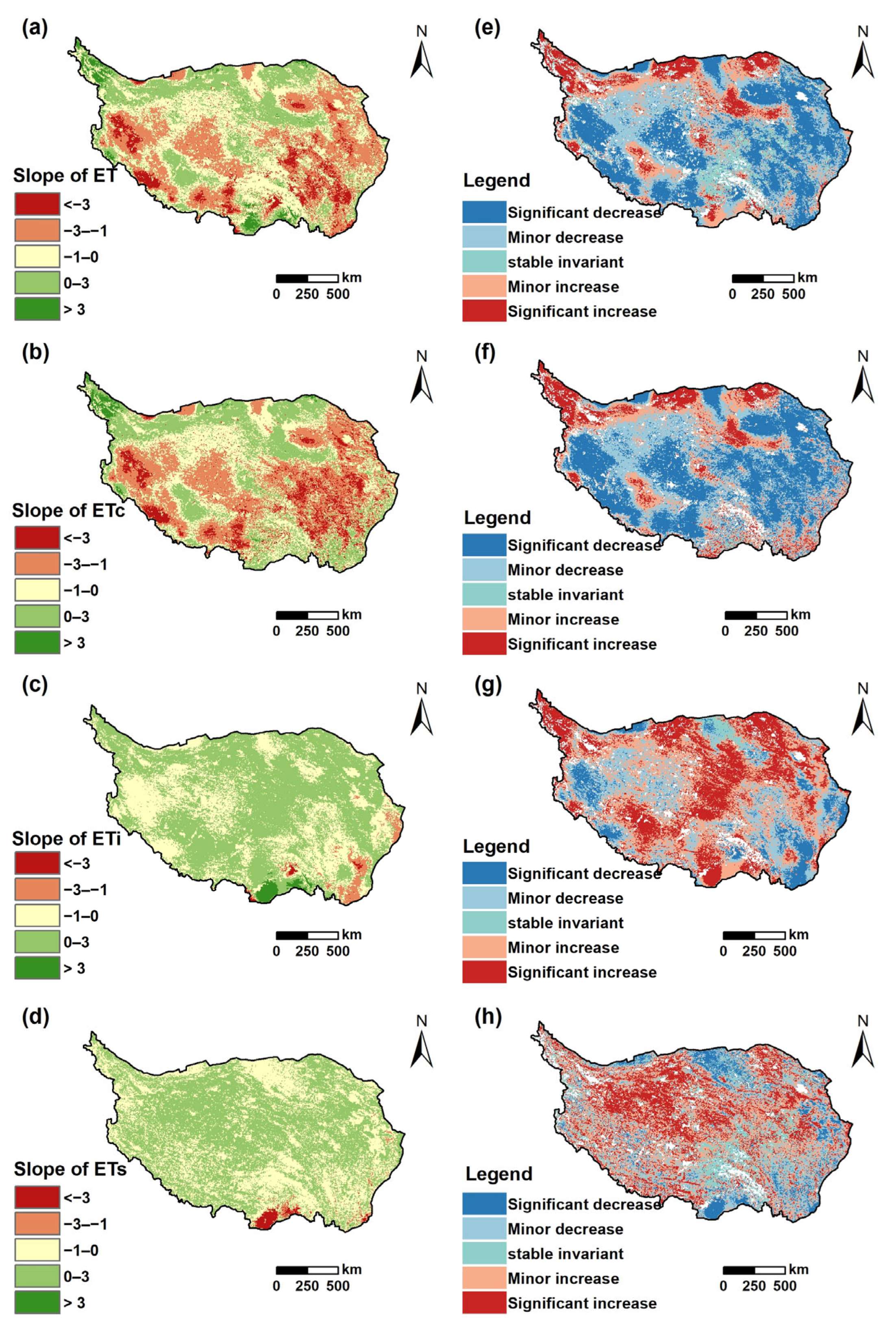
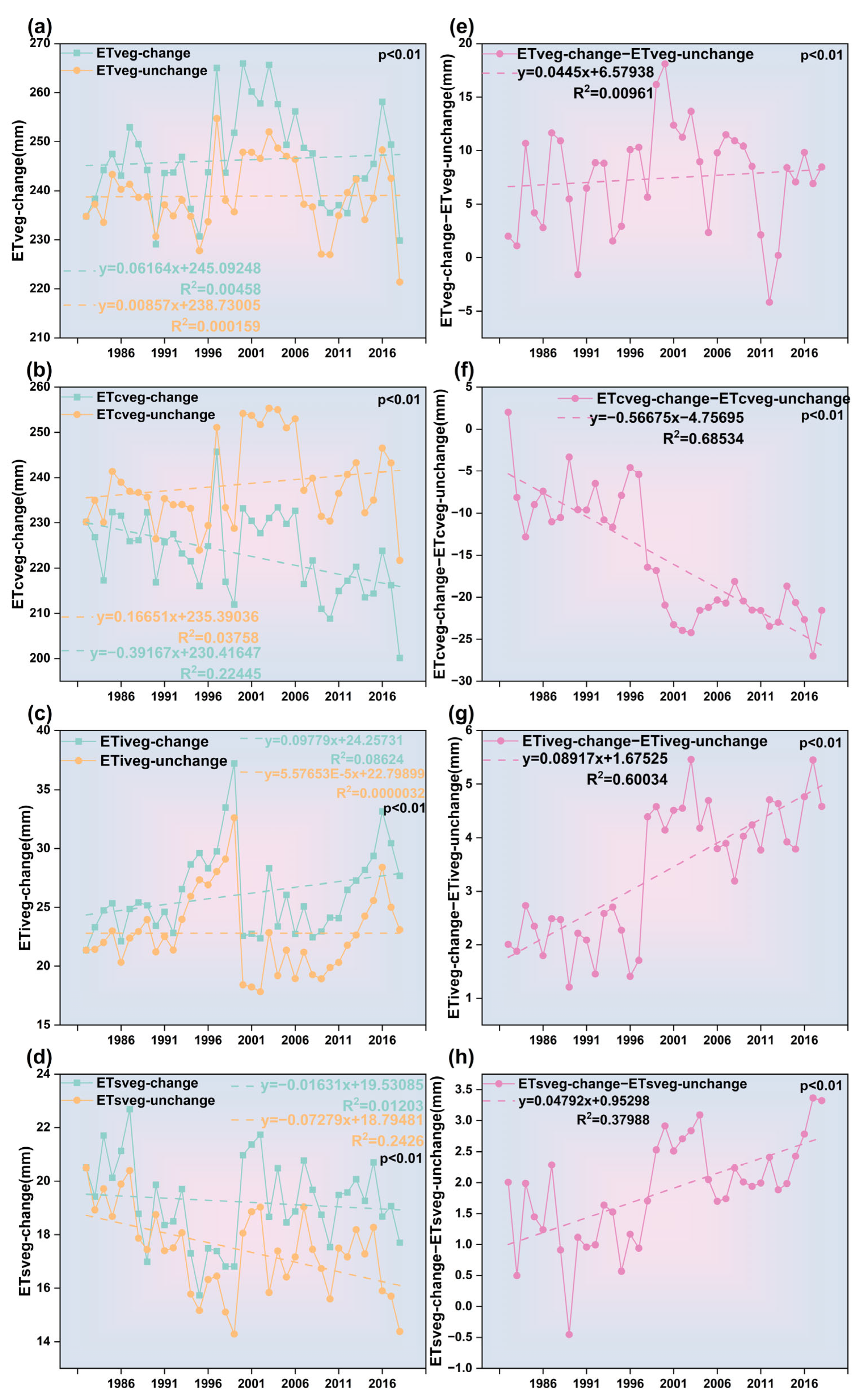
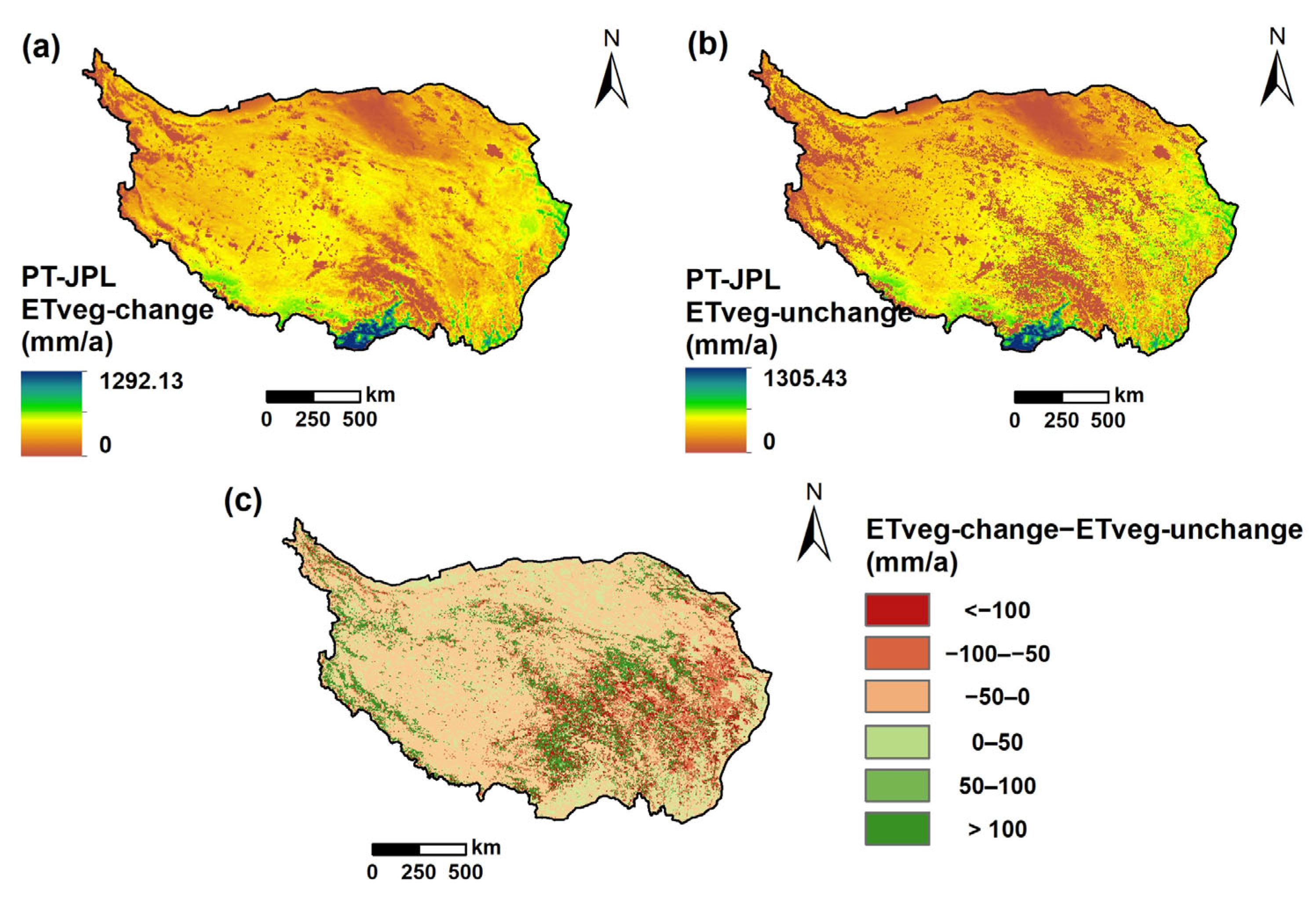
3.4. Net Effect of Vegetation Changes on ET and Its Components

Figure 8a depicts the interannual dynamics of ET across the TP under both vegetation change and static vegetation scenarios during 1982–2018. The results indicate that ET levels were generally elevated when vegetation change was considered, exhibiting a statistically significant average annual increase of 0.06 mm/year (p < 0.01); as shown in Figure 8a, this trend corresponds to the linear slope shown in Figure 8a (y = 0.06164x + 245.09). Between 1982 and 1987, ET rose gradually, followed by a notable decline from 1987 to 1990. A peak occurred in 1997, after which elevated ET values persisted for approximately five years. Throughout the study period, the mean annual difference between the two scenarios was 7.4 mm, with the largest gap of 18 mm observed around 2001. Exceptions occurred in 1990 and 2012, when the ET in the static vegetation scenario surpassed that of the changing vegetation scenario. For canopy transpiration (ETc), a consistent upward trend was observed under the vegetation change scenario, whereas the unchanged vegetation case displayed a more pronounced downward trajectory (p < 0.05). The divergence between the two progressively widened over time, reaching its lowest relative peak in 2017. Interception evaporation (ETi) increased in both scenarios prior to 2000, followed by a sharp decline thereafter. Although the overall difference in ETi was relatively small, the vegetation change scenario consistently yielded higher values, with the gap expanding at a rate of approximately 0.1 mm per year. Regarding soil evaporation (ETs), both scenarios exhibited a general downward trend across the 37-year period. Nevertheless, the ET values remained slightly higher under the vegetation change scenario, with the inter-scenario difference growing gradually at a rate of 0.04 mm per year—slightly less than that observed for ETi.

The divergent trends between the vegetation change and static vegetation scenarios, as shown in Figure 8, can be primarily attributed to the interplay between vegetation dynamics and climatic drivers. Regions exhibiting substantial greening (Figure 5) experienced notable increases in canopy transpiration (ETc), which elevated the total ET under the vegetation change scenario. In contrast, under static vegetation conditions, ET trends were more strongly controlled by climatic factors such as precipitation and vapor pressure deficit (VPD), leading to spatially heterogeneous ET responses.

Specifically, in areas where vegetation greening was pronounced and climatic conditions remained relatively stable, the increase in ETc dominated the ET trend, resulting in overall positive ET changes. Conversely, in regions where climatic stress intensified (e.g., rising VPD or declining precipitation), even with modest vegetation growth, the total ET did not increase substantially or even declined, highlighting the limitation of vegetation buffering under intensified climatic aridity.

Furthermore, the components of ET responded differently to vegetation and climate interactions. ETc was highly sensitive to changes in LAI and canopy greenness, while ETi (interception evaporation) was more influenced by precipitation patterns. Soil evaporation (ETs) exhibited complex behaviors, decreasing in severely water-limited regions and increasing where soil moisture availability was improved. These findings suggest that vegetation dynamics not only amplify transpiration but also modulate the sensitivity of different ET components to climatic variability.

Figure 9 displays the spatial distribution of multi-year mean ET across the TP from 1982 to 2018 under both vegetation change and static scenarios. Under the vegetation change condition, the southern TP recorded the highest ET levels, exceeding 800 mm, while ET sharply declined northward, falling below 300 mm in many areas. Notably, 95.2% of the TP exhibited mean ET values under 400 mm. In the vegetation-invariant scenario (Figure 9b), southern TP regions also experienced ET above 800 mm; however, only 9.3% of the total area exceeded 400 mm, indicating a more constrained spatial extent of high ET values. A south-to-north and periphery-to-center decreasing trend in ET was observed in both scenarios, yet areas with ET below 300 mm were more widespread in the vegetation change case. Figure 9c compares the two scenarios by mapping the difference in multi-year mean ET. The actual ET values, when vegetation change is accounted for, were lower than those simulated under the static scenario, particularly in forest-dominated regions, where differences exceeded 100 mm. Overall, 74.1% of the TP area showed lower ET under the vegetation change scenario, highlighting the spatially heterogeneous impacts of vegetation dynamics on long-term ET distribution. While most areas exhibit positive differences in ET under vegetation change, certain pixels present negative values. These reductions are primarily attributed to decreases in canopy transpiration (ETc), particularly in regions where vegetation dynamics were weak or negative. Such areas may include high-elevation zones or semi-arid patches where vegetation greening was minimal, and increased atmospheric demand (e.g., VPD) suppressed ET.

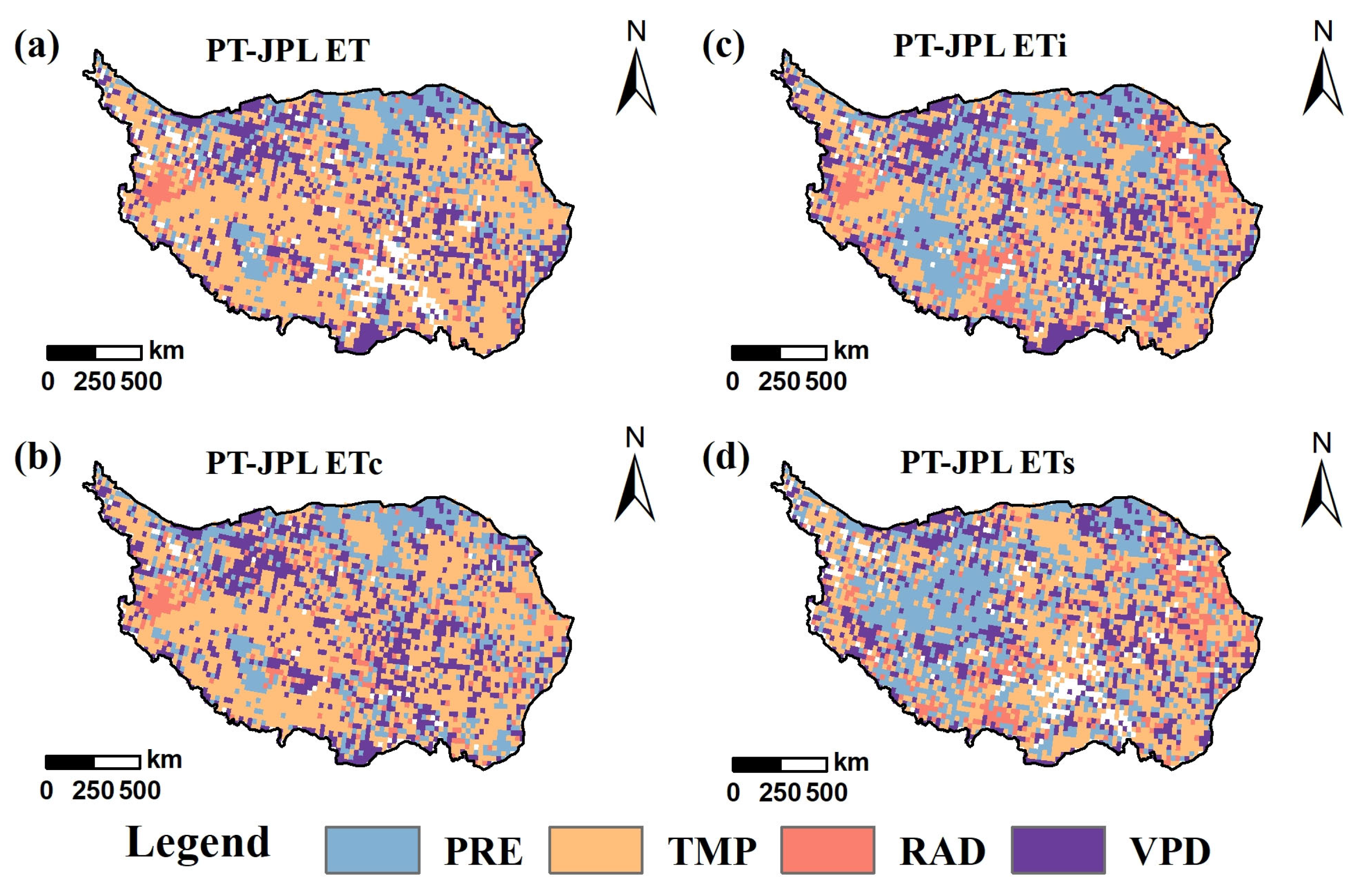
3.5. Spatiotemporal Trends of Climatic Drivers and Their Influence on ET

Changes in ET across the TP are influenced not only by vegetation dynamics but also by variations in atmospheric water availability and energy-related climatic drivers. While the previous sections have quantified the contribution of vegetation changes over the 37-year period, this section focuses on assessing the impact of climate variability on ET through a multiple regression framework. As illustrated in Figure 10, four key climatic variables—precipitation (PRE), temperature (TMP), radiation (RAD), and vapor pressure deficit (VPD)—exhibit distinct spatial and temporal trends across the TP. Figure 10a maps the Sen–Mann–Kendall (Sen-MK) trend in PRE, revealing that 99.7% of the region experienced a statistically significant increase, particularly evident in a southeast-to-northwest gradient. The interannual trend of PRE (Figure 10i) reflects a rise from 304.4 mm to 348.29 mm over the study period, corresponding to an average annual increase of 0.5 mm. Temperature trends (Figure 10b) derived from the Mann–Kendall (MK) test show that 72.2% of the TP underwent either moderate or significant warming. Spatially, a decreasing gradient in warming trends is observed from the central plateau toward peripheral regions. Annual TMP values increased from −3.2 °C to −2.3 °C (Figure 10j), with an average increment of 0.03 °C per year. Figure 10c presents RAD trends, where 78.2% of the TP exhibited significant increases, most notably originating from central areas. Despite the overall positive trend (86.8% of the area), a notable decline in RAD was observed in southern regions. Annual average RAD values rose from 63.1 to 64.5 W/m², with a mean yearly increase of 0.04 W/m² (Figure 10k). VPD trends, as shown in Figure 10d, reveal a more spatially heterogeneous pattern. Roughly 47.8% of the plateau showed increasing VPD values, characterized by a stepwise gradient from west to east. The line graph in Figure 10l shows a subtle rise in annual VPD, from 0.31 to 0.32 kPa, averaging an annual increase of 0.001 kPa/year.

Figure 11 presents the spatial distribution of contributions from four climatic variables—precipitation (PRE), temperature (TMP), radiation (RAD), and vapor pressure deficit (VPD)—to variations in total ET and its components (ETc, ETi, ETs) across the TP over the past 37 years. For total ET (Figure 11a–d), PRE emerged as the dominant positive contributor, with an average effect of +0.48 mm/year and localized values reaching up to +2 mm/year in the central TP. TMP and VPD exerted negative influences overall, averaging −0.13 mm/year and −0.05 mm/year, respectively. TMP contributed positively to ET in 35.9% of the region, primarily in central, western, and parts of southeastern TP, whereas stronger negative impacts (less than −3 mm/year) were concentrated in the southern TP. RAD exhibited a relatively modest influence, remaining within the range of −0.5 to +0.5 mm/year for 97.5% of the region. For canopy transpiration (ETc, Figure 11e–h), the average contributions of PRE, TMP, RAD, and VPD were +4.28, −5.30, +0.36, and −0.06 mm/year, respectively. TMP and VPD were the main suppressors of ETc, with widespread reductions observed across the plateau. While RAD showed a minor enhancing effect in northern and northwestern TP (0–3 mm/year), it had a weakening influence in the central regions, averaging around −0.5 mm/year. Regarding interception evaporation (ETi, Figure 11i–l), TMP had the strongest enhancing impact, with an average contribution of +1.27 mm/year, followed by PRE at +0.41 mm/year. These positive trends were observed in more than 62% of the TP, especially across eastern, southern, and central zones. RAD and VPD contributed marginally, with VPD still showing a weak negative influence (−0.23 mm/year on average). As for soil evaporation (ETs), climatic influences were comparatively weak. The mean contributions of PRE, TMP, RAD, and VPD were +0.004, −0.39, −0.01, and +0.03 mm/year, respectively. TMP’s role was more spatially variable, particularly across central and southwestern TP, while the other factors remained largely within the ±0.5 mm/year range. In summary, while RAD exhibited limited spatial impact across all components, the contributions from PRE, TMP, and VPD varied significantly in magnitude and direction, exerting dominant roles in shaping the long-term ET dynamics of the TP.

To better understand the climatic controls on ET and its components across the TP, we conducted a dominant factor analysis under the vegetation change scenario using the PT-JPL model. Specifically, four key climatic drivers—precipitation (PRE), temperature (TMP), radiation (RAD), and vapor pressure deficit (VPD)—were assessed for their relative influence on ET, canopy transpiration (ETc), interception evaporation (ETi), and soil evaporation (ETs). Unlike the multiple linear regression results presented in Figure 11, which quantify the continuous contribution of each climatic variable to ET trends, the dominant factor analysis shown in Figure 12 identifies the single most influential driver at each pixel. This classification was determined based on the variable with the highest standardized contribution value to the overall ET trend, using the method adapted from [58]. The approach allows for spatially explicit attribution of ET dynamics to dominant climate controls across the TP. As shown in Figure 12, TMP emerged as the leading driver of total ET variation, accounting for 53.5% of the TP’s area. VPD followed as the dominant factor over 23.0% of the region, with PRE and RAD influencing 18.0% and 5.5% of the area, respectively. For ETc, TMP continued to play the dominant role, though its spatial coverage declined slightly to 51.7%. In the case of ETi and ETs, the relative importance of TMP decreased more substantially, while the spatial extent dominated by RAD and PRE expanded markedly—by over 53.6% and 88.2%, respectively. VPD’s influence remained relatively stable, covering around 22% of the region for all components. Spatially, TMP dominated in most regions except for the northern and northeastern fringes of the TP. PRE exhibited dominance primarily in the northern and northeastern zones of the TP, while RAD exerted its strongest influence in the far western region, particularly around the Ali area. VPD showed a more fragmented distribution, with dominant patches scattered across various parts of the plateau.

4. Discussion

4.1. Evaluation of ET and Its Components Based on PT-JPL Simulations and Spatiotemporal Patterns

The simulated ET using the PT-JPL model demonstrates strong consistency with both flux tower observations at three representative sites and GLEAM-based ET estimates across the TP, as shown in Figure 2, Figure 3 and Figure 4. The model-estimated mean annual ET over the TP during 1982–2018 reached 246.3 mm, which is comparable to previously reported values [59]. The relatively low average ET value (246.3 mm/year) in our study compared to previous studies [60,61] can be attributed to several factors. First, our study covers the entire TP, including vast arid and sparsely vegetated areas with inherently low ET. Second, the PT-JPL model tends to yield conservative ET estimates in water-limited regions due to its simplified parameterization of soil evaporation and interception. Third, spatial resolution plays a critical role: our PT-JPL implementation uses inputs at 0.25°, which is already finer than many global products (e.g., GLEAM at 0.25° or coarser), but still coarse relative to the spatial heterogeneity of the TP. However, PT-JPL allows for flexible integration of higher-resolution remote sensing data (e.g., MODIS LAI, NDVI, albedo), making it more suitable for scaling up in future fine-resolution studies. In contrast, previous studies often focused on vegetation-dense subregions or used alternative models with more aggressive soil evaporation modules. For example, an average ET of 411.7 mm for 2001–2018 was estimated using the MEP model for the Three Rivers Source region, an area characterized by higher vegetation density in the eastern and southern TP [62]. This explains the higher regional value compared to our plateau-wide average. Differences among ET estimates across studies may stem from variability in input datasets, spatial resolutions, model configurations, and study periods [63]. Notably, in complex mountainous regions like the TP, model suitability is strongly tied to how well spatial heterogeneity can be resolved and parameterized. Recent advancements, such as the integration of physical constraints with machine learning frameworks, have shown promise in improving satellite-based ET estimates over the TP [64]. These approaches offer enhanced representation of nonlinear land–atmosphere interactions and may serve as valuable complements or alternatives to traditional physically based models like PT-JPL. For example, although specific ET values were not published, a modified MOD16-based simulation showed 8-day average values in 2010 (approximately 25 mm) that closely match our PT-JPL-derived result of 22 mm over the same period [59]. Furthermore, a downward trend in terrestrial water storage change (TWSC) across 80% of the S05 subregion—including the junction of the Bayankala and Tanggula Mountains—was identified using the random forest (RF) method [65], which is consistent with our simulated results for water availability changes. These comparisons underscore the reliability of the PT-JPL model in simulating ET and related hydrological dynamics across the TP. Its outputs are well-aligned with various independent studies, further supporting its robustness in representing long-term water balance shifts.

Overall, the modeled values of ET and its components (ETc, ETi, ETs) fall within a reasonable range, corroborated by previous findings [59,66,67]. However, minor discrepancies were observed when compared with GLEAM-derived ET, particularly in the magnitude of seasonal peaks. Two primary factors account for this divergence. First, although PT-JPL accounts for physiological and ecological drivers of ET, it provides limited consideration for soil moisture constraints. This may result in overestimated ET in arid areas where water availability is low [68]. In contrast, GLEAM explicitly incorporates soil moisture effects across three stratified layers—vegetated areas, sparsely vegetated regions, and bare soil—which allows for more nuanced ET estimation under heterogeneous land surface conditions [69,70]. Second, PT-JPL utilizes the Leaf Area Index (LAI) to partition net radiation into soil-absorbed (RAD-soil) and canopy-intercepted (RAD-c) components, whereas GLEAM does not differentiate these energy pathways [71]. Accordingly, the observed deviations between PT-JPL and GLEAM ET components likely reflect differences in both soil moisture coupling and energy balance representation.

4.2. Effects of Vegetation Dynamics and Climatic Drivers on ET and Its Component Processes

Our comparison between dynamic and static vegetation scenarios revealed that vegetation greening significantly enhanced ET across the TP. Over the study period (1982–2018), total ET under vegetation change conditions increased at a rate of approximately 0.06 mm/year, compared to only 0.01 mm/year under the static vegetation scenario (Figure 8a). The net water consumption effect of greening was quantified as an average increase of 0.04 mm/year (Figure 8e), with 74.1% of the TP exhibiting higher ET under dynamic vegetation, particularly in the central and western regions where the annual mean ET difference exceeded 100 mm. The average ET under dynamic vegetation reached 258.6 ± 120.9 mm, 2.9% higher than that under static conditions (251.2 ± 157.2 mm). These results suggest that enhanced vegetation cover promoted transpiration and interception processes, as also shown in the spatial patterns of ET components (Figure 6 and Figure 7).

Our findings align with previous studies emphasizing the importance of vegetation in regulating ET, though regional differences are evident. For instance, while studies in the Yellow River Basin attributed a 1.58 mm/year increase in ET to vegetation dynamics, they found soil evaporation (ETs) to be the dominant component, accounting for 77% of total ET [26,72]. In contrast, our analysis shows that canopy transpiration (ETc) is the major contributor on the TP, likely due to its high elevation and sparse surface moisture. These findings underscore the spatial heterogeneity of vegetation impacts on water fluxes across different ecological zones. Notably, Leaf Area Index (LAI) increased across 64.8% of the TP (Figure 5f), closely tied to ecological restoration policies implemented in recent decades [73].

Climatic drivers also played a crucial role in shaping ET dynamics. From 1982 to 2018, precipitation (PRE), temperature (TMP), radiation (RAD), and vapor pressure deficit (VPD) all exhibited upward trends, reflecting broader signals of climate warming, glacial retreat, and increasing atmospheric water demand [74]. Periods such as 1986–1996 showed synchronized declines in these variables, resulting in corresponding reductions in ET and its components—a pattern consistent with prior research [67]. Figure 11 shows that TMP exerted the strongest negative influence on ETc across most of the plateau, while PRE and RAD had more localized positive contributions. Dominant factor analysis (Figure 12) further revealed that TMP was the primary climatic control of ET in 53.5% of the TP, followed by VPD (23%), PRE (18%), and RAD (5.5%). Spatially, TMP dominated in western and central regions with limited vegetation, while PRE and RAD exhibited stronger influence in northern and northwestern zones such as Ali and Haixi. The spatial dominance of VPD and its increasing trend over the past four decades are consistent with the findings of Xu, et al. [75], who highlighted rising atmospheric evaporative demand as a major constraint on surface water availability in the TP.

Finally, the positive association between vegetation indices (NDVI, LAI) and ET trends across the central and eastern TP suggests that greening not only increased vegetation density but also enhanced the land–atmosphere water and energy exchanges [76]. Compared with previous estimates such as Ma and Zhang [60], who reported a higher mean ET (353 mm/year), our estimate (246.3 mm/year) was lower due to differences in model structure, spatial resolution, and study domain. Crucially, our study explicitly isolated the role of vegetation by comparing dynamic and static scenarios, whereas previous studies often integrated vegetation change implicitly. The inclusion of sparsely vegetated and arid areas in our analysis also contributed to the lower average values. Overall, these findings demonstrate that vegetation greening, combined with climatic shifts, has significantly modified ET patterns across the TP during the past four decades.

4.3. Ecological Insights and Strategic Recommendations for Vegetation Recovery and Water Management

This study highlights how grassland greening and climate dynamics together regulate ET, altering ecosystem functions, hydrological balance, and water availability. Previous research has demonstrated that changes in ET can substantially influence streamflow and groundwater recharge patterns, with direct implications for watershed-scale water security [77]. An observed long-term increase in ET across the TP, particularly over recent decades, has already begun to reshape basin-scale hydrological regimes [78]. These evolving patterns pose new challenges for the formulation and implementation of water governance frameworks.

Importantly, our results show that among the three ET components, canopy transpiration (ETc) was the dominant contributor to the increase in total ET under vegetation change scenarios, accounting for approximately **65%** of the net ET increase from 1982 to 2018. In contrast, soil evaporation (ETs) and canopy interception (ETi) contributed around **25%** and **10%**, respectively. This partitioning indicates that vegetation water use—primarily through transpiration—is increasingly responsible for water consumption in greening zones. Such trends suggest that continued vegetation restoration without water-adaptive strategies may exacerbate dry-season water shortages or alter baseflow dynamics, especially in semiarid and high-altitude regions where water availability is limited.

To address these issues, the following adaptive strategies are recommended: (1) Improve irrigation efficiency by adopting water-saving technologies and optimizing irrigation schedules, particularly in agricultural zones where water demand is high. (2) Expand water storage infrastructure, such as reservoirs and high-altitude ponds, to buffer against seasonal water scarcity and support dry-season supply stability. (3) Promote policy-driven conservation measures, including legal frameworks and public education campaigns aimed at fostering a culture of efficient and sustainable water use. These actions are expected to strengthen ecological resilience and contribute to long-term sustainability in the TP’s fragile alpine environment. Building on our results, we further recommend region-specific strategies for future afforestation and reforestation efforts. In relatively humid regions, particularly the southeastern TP, where water availability is more reliable, vegetation expansion can enhance ecosystem services without critically depleting water resources [16,64]. Conversely, in semi-arid and high-altitude zones in the northwestern TP, afforestation efforts should be approached cautiously, as excessive greening could exacerbate water scarcity due to the already limited precipitation and high evaporative demand [75]. Implementing water-adaptive management practices, such as selecting drought-tolerant species and optimizing planting density, will be essential in these vulnerable areas to balance ecological restoration goals with regional hydrological sustainability. Given the complex spatial and temporal patterns observed over the 1982–2018 period, continued monitoring and interdisciplinary research are vital. Establishing a robust, long-term observational network will support more accurate predictions and adaptive decision-making in the face of ongoing climate variability and ecological transformation.

4.4. Uncertainties and Limitations

Despite methodological advancements, a key limitation is the lack of rigorous quality control of input datasets, which introduces uncertainties. Our model isolated vegetation effects, though in reality, vegetation and meteorological factors interact [79,80]. During vegetation greening in some areas of TP, the original dynamic equilibrium between vegetation and water resources was disrupted because the principle of balancing vegetation greening with water supply and demand was not followed. Excessive vegetation greening has significantly depleted soil water resources, causing ecological issues such as soil drying and vegetation degradation. Simultaneously, vegetation changes and greening processes, such as afforestation, may alter soil properties by leading to the accumulation of leaf litter on the surface and the development of subsurface root systems [81]. And the simple use of dynamic vegetation parameters cannot accurately represent the complex changes of land use types. Further refinement of the PT-JPL model outputs remains essential to enhance simulation accuracy. A key limitation lies in the limited availability and uneven spatial distribution of flux tower-derived ET data, which hampers comprehensive model calibration and validation. To address this gap, expanding the flux tower network—particularly in regions sensitive to climatic and vegetation changes—is critical for improving the observational basis required for regional ET assessments. While our analysis focuses on annual-scale trends, we acknowledge that climatic drivers such as temperature, precipitation, and vapor pressure deficit exhibit pronounced seasonal variability. This seasonal heterogeneity may modulate ET dynamics in ways that are not fully captured by annual aggregates. Future research should therefore extend the current framework to explore seasonal patterns of ET and its components, improving our understanding of short-term ecosystem-climate interactions on the TP.

5. Conclusions

This study employed the PT-JPL model to estimate ET and its components—canopy transpiration (ETc), interception evaporation (ETi), and soil evaporation (ETs)—across the TP, assessing the respective contributions of vegetation greening and climatic changes from 1982 to 2018. The key findings are summarized as follows:

(1)

Model Performance and Vegetation-Induced Effects: The PT-JPL model successfully captured spatial and temporal variations in ET over the TP under vegetation change conditions. The estimated linear trends of ET, ETc, ETi, and ETs were 0.06, 0.39, 0.005, and 0.07 mm/year, respectively. Vegetation greening notably intensified ET, resulting in an annual ET increase of 2.9% compared to the scenario without vegetation change (258.6 ± 120.9 mm vs. 251.2 ± 157.2 mm), thereby indicating greater evaporative water consumption associated with enhanced vegetation cover.

(2)

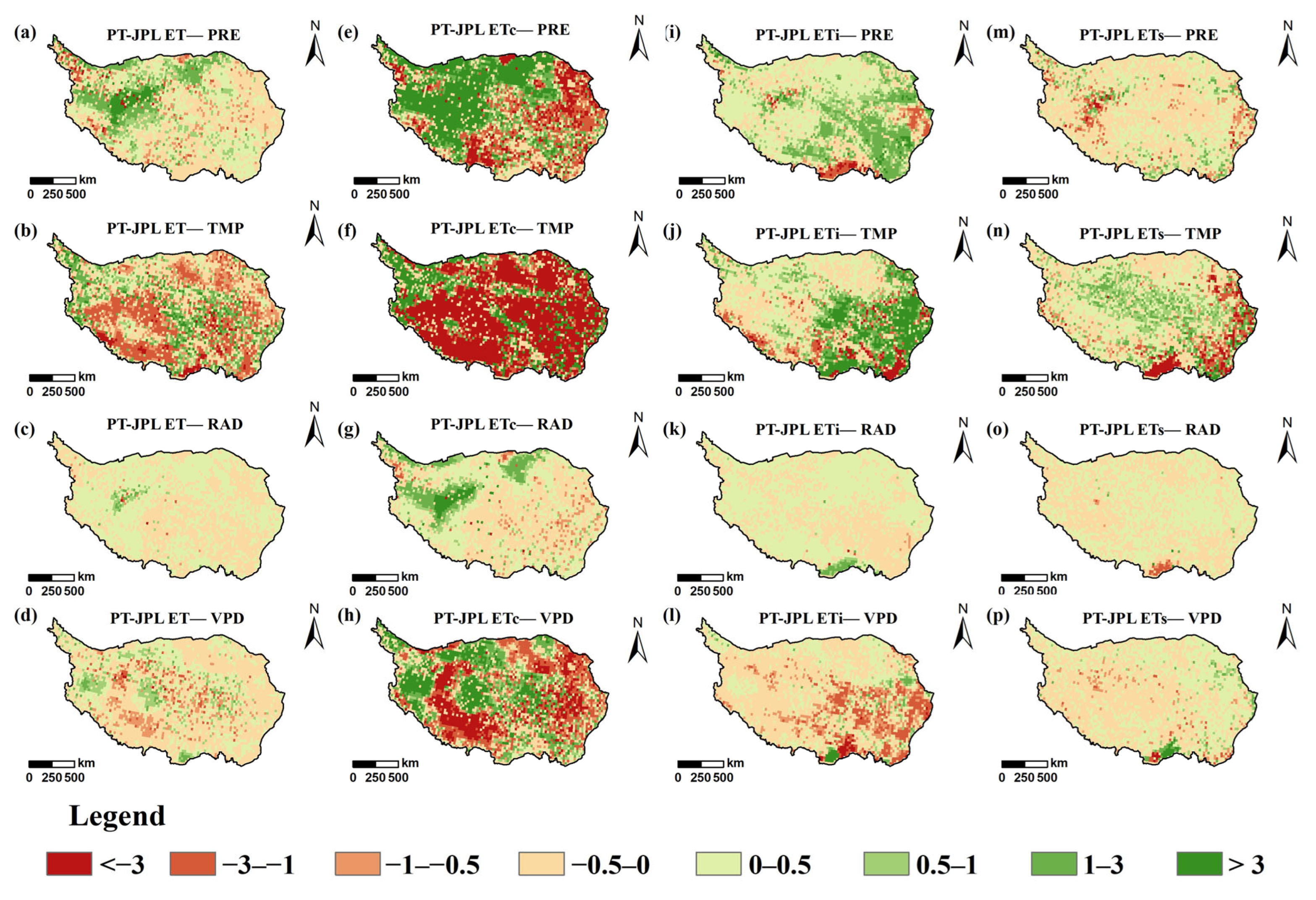
Climate Factors and Dominant Influences: Temperature (TMP) and vapor pressure deficit (VPD) were the primary climatic factors influencing ET and its components. The average contributions of PRE, TMP, RAD, and VPD to ET changes were 0.48, −0.13, 0.04, and −0.05 mm/year, respectively. TMP was the dominant factor affecting ET changes in 53.5% of the TP area, while VPD dominated in 23.0%, PRE in 18.0%, and RAD in 5.5%.

(3)

Implications for Water Resource Management: The results underscore the considerable influence of vegetation greening and climatic shifts on ET in the TP. These findings offer actionable guidance for sustainable vegetation restoration and regional water management. Priority should be given to adaptive measures such as improving irrigation efficiency, expanding water storage infrastructure, and promoting policy frameworks for water conservation.

In summary, this research delivers an integrated assessment of how vegetation dynamics and climate variability affect ET and its components in the TP. The outcomes not only advance scientific understanding of ecohydrological interactions in high-altitude environments but also serve as a foundation for formulating evidence-based strategies in future ecological management and policy development. Although this study provides robust insights into long-term vegetation and climate effects on ET, it does not resolve the seasonal variations of these drivers. Future studies should incorporate seasonal-scale analyses to elucidate how intra-annual climatic fluctuations shape ET dynamics and inform more precise water resource management strategies.

References

1. Suliman, M.; Scaini, A.; Manzoni, S.; Vico, G. Soil properties modulate actual evapotranspiration and precipitation impacts on crop yields in the USA. Sci. Total Environ. 2024, 949, 175172. [Google Scholar] [CrossRef] [PubMed]
2. García, A.G.; Di Bella, C.M.; Houspanossian, J.; Magliano, P.N.; Jobbágy, E.G.; Posse, G.; Fernández, R.J.; Nosetto, M.D. Patterns and controls of carbon dioxide and water vapor fluxes in a dry forest of central Argentina. Agric. For. Meteorol. 2017, 247, 520–532. [Google Scholar] [CrossRef]
3. Zeng, Z.; Peng, L.; Piao, S. Response of terrestrial evapotranspiration to Earth’s greening. Curr. Opin. Environ. Sustain. 2018, 33, 9–25. [Google Scholar] [CrossRef]
4. Fisher, J.B.; Melton, F.; Middleton, E.; Hain, C.; Anderson, M.; Allen, R.; McCabe, M.F.; Hook, S.; Baldocchi, D.; Townsend, P.A.; et al. The future of evapotranspiration: Global requirements for ecosystem functioning, carbon and climate feedbacks, agricultural management, and water resources. Water Resour. Res. 2017, 53, 2618–2626. [Google Scholar] [CrossRef]
5. Walker, G.R.; Hughes, M.W.; Allison, G.B.; Barnes, C.J. The movement of isotopes of water during evaporation from a bare soil surface. J. Hydrol. 1988, 97, 181–197. [Google Scholar] [CrossRef]
6. Lan, X.; Liu, Z.; Chen, X.; Lin, K.; Cheng, L. Trade-off between carbon sequestration and water loss for vegetation greening in China. Agric. Ecosyst. Environ. 2021, 319, 107522. [Google Scholar] [CrossRef]
7. Schlesinger, W.H.; Jasechko, S. Transpiration in the global water cycle. Agric. For. Meteorol. 2014, 189–190, 115–117. [Google Scholar] [CrossRef]
8. Wei, Z.; Yoshimura, K.; Wang, L.; Miralles, D.G.; Jasechko, S.; Lee, X. Revisiting the contribution of transpiration to global terrestrial evapotranspiration. Geophys. Res. Lett. 2017, 44, 2792–2801. [Google Scholar] [CrossRef]
9. Xu, S.; Yu, Z.; Yang, C.; Ji, X.; Zhang, K. Trends in evapotranspiration and their responses to climate change and vegetation greening over the upper reaches of the Yellow River Basin. Agric. For. Meteorol. 2018, 263, 118–129. [Google Scholar] [CrossRef]
10. Marimon-Junior, B.H.; Hay, J.D.V.; Oliveras, I.; Jancoski, H.; Umetsu, R.K.; Feldpausch, T.R.; Galbraith, D.R.; Gloor, E.U.; Phillips, O.L.; Marimon, B.S. Soil water-holding capacity and monodominance in Southern Amazon tropical forests. Plant Soil 2020, 450, 65–79. [Google Scholar] [CrossRef]
11. Cui, Y.; Jia, L. Estimation of evapotranspiration of “soil-vegetation” system with a scheme combining a dual-source model and satellite data assimilation. J. Hydrol. 2021, 603, 127145. [Google Scholar] [CrossRef]
12. Xue, Y.; Liang, H.; Zhang, H.; Yin, L.; Feng, X. Quantifying the policy-driven large scale vegetation restoration effects on evapotranspiration over drylands in China. J. Environ. Manag. 2023, 345, 118723. [Google Scholar] [CrossRef] [PubMed]
13. Yang, Z.; Bai, P.; Li, Y. Quantifying the effect of vegetation greening on evapotranspiration and its components on the Loess Plateau. J. Hydrol. 2022, 613, 128446. [Google Scholar] [CrossRef]
14. Zhou, H.; Ma, L.; Niu, X.; Xiang, Y.; Chen, J.; Su, Y.; Li, J.; Lu, S.; Chen, C.; Wu, Q. A novel hybrid model combined with ensemble embedded feature selection method for estimating reference evapotranspiration in the North China Plain. Agric. Water Manag. 2024, 296, 108807. [Google Scholar] [CrossRef]
15. Yu, L.; Liu, Y.; Liu, T.; Yan, F. Impact of recent vegetation greening on temperature and precipitation over China. Agric. For. Meteorol. 2020, 295, 108197. [Google Scholar] [CrossRef]
16. Yang, Y.; Roderick, M.L.; Guo, H.; Miralles, D.G.; Zhang, L.; Fatichi, S.; Luo, X.; Zhang, Y.; McVicar, T.R.; Tu, Z.; et al. Evapotranspiration on a greening Earth. Nat. Rev. Earth Environ. 2023, 4, 626–641. [Google Scholar] [CrossRef]
17. Łopucki, R.; Klich, D.; Kociuba, P. Detection of spatial avoidance between sousliks and moles by combining field observations, remote sensing and deep learning techniques. Sci. Rep. 2022, 12, 8264. [Google Scholar] [CrossRef]
18. Holland, S.; Heitman, J.L.; Howard, A.; Sauer, T.J.; Giese, W.; Ben-Gal, A.; Agam, N.; Kool, D.; Havlin, J. Micro-Bowen ratio system for measuring evapotranspiration in a vineyard interrow. Agric. For. Meteorol. 2013, 177, 93–100. [Google Scholar] [CrossRef]
19. Ghisi, T.; Fischer, M.; Nieto, H.; Kowalska, N.; Jocher, G.; Homolová, L.; Burchard-Levine, V.; Žalud, Z.; Trnka, M. Evaluation of the METRIC and TSEB remote sensing evapotranspiration models in the floodplain area of the Thaya and Morava Rivers. J. Hydrol. Reg. Stud. 2024, 53, 101785. [Google Scholar] [CrossRef]
20. Mondal, I.; Thakur, S.; De, A.; De, T.K. Application of the METRIC model for mapping evapotranspiration over the Sundarban Biosphere Reserve, India. Ecol. Indic. 2022, 136, 108553. [Google Scholar] [CrossRef]
21. Bečanová, J.; Komprdová, K.; Vrana, B.; Klánová, J. Annual dynamics of perfluorinated compounds in sediment: A case study in the Morava River in Zlín district, Czech Republic. Chemosphere 2016, 151, 225–233. [Google Scholar] [CrossRef] [PubMed]
22. O’Donncha, F.; Hu, Y.; Palmes, P.; Burke, M.; Filgueira, R.; Grant, J. A spatio-temporal LSTM model to forecast across multiple temporal and spatial scales. Ecol. Inform. 2022, 69, 101687. [Google Scholar] [CrossRef]
23. Fisher, J.B.; Tu, K.P.; Baldocchi, D.D. Global estimates of the land–atmosphere water flux based on monthly AVHRR and ISLSCP-II data, validated at 16 FLUXNET sites. Remote Sens. Environ. 2008, 112, 901–919. [Google Scholar] [CrossRef]
24. Elfarkh, J.; Johansen, K.; El Hajj, M.M.; Almashharawi, S.K.; McCabe, M.F. Evapotranspiration, gross primary productivity and water use efficiency over a high-density olive orchard using ground and satellite based data. Agric. Water Manag. 2023, 287, 108423. [Google Scholar] [CrossRef]
25. Li, X.; Zou, L.; Xia, J.; Zhang, L.; Wang, F.; Li, M. Response of blue-green water to climate and vegetation changes in the water source region of China’s South-North water Diversion Project. J. Hydrol. 2024, 634, 131061. [Google Scholar] [CrossRef]
26. Jiang, X.; Wang, Y.; Yinglan, A.; Wang, G.; Zhang, X.; Ma, G.; Duan, L.; Liu, K. Optimizing actual evapotranspiration simulation to identify evapotranspiration partitioning variations: A fusion of physical processes and machine learning techniques. Agric. Water Manag. 2024, 295, 108755. [Google Scholar] [CrossRef]
27. Kimball, B.A.; Thorp, K.R.; Boote, K.J.; Stockle, C.; Suyker, A.E.; Evett, S.R.; Brauer, D.K.; Coyle, G.G.; Copeland, K.S.; Marek, G.W.; et al. Simulation of evapotranspiration and yield of maize: An inter-comparison among 41 maize models. Agric. For. Meteorol. 2023, 333, 109396. [Google Scholar] [CrossRef]
28. Ehlers, T.A.; Chen, D.; Appel, E.; Bolch, T.; Chen, F.; Diekmann, B.; Dippold, M.A.; Giese, M.; Guggenberger, G.; Lai, H.-W.; et al. Past, present, and future geo-biosphere interactions on the Tibetan Plateau and implications for permafrost. Earth-Sci. Rev. 2022, 234, 104197. [Google Scholar] [CrossRef]
29. Dong, S.; Shang, Z.; Gao, J.; Boone, R. Enhancing the ecological services of the Qinghai-Tibetan Plateau’s grasslands through sustainable restoration and management in era of global change. Agric. Ecosyst. Environ. 2022, 326, 107756. [Google Scholar] [CrossRef]
30. Guo, Z.; Huang, N.; Dong, Z.; Van Pelt, R.S.; Zobeck, T.M. Wind Erosion Induced Soil Degradation in Northern China: Status, Measures and Perspective. Sustainability 2014, 6, 8951–8966. [Google Scholar] [CrossRef]
31. Wang, J.; Zhang, C.; Luo, P.; Yang, H.; Luo, C. Water yield response to plant community conversion caused by vegetation degradation and improvement in an alpine meadow on the northeastern Tibetan Plateau. Sci. Total Environ. 2023, 856, 159174. [Google Scholar] [CrossRef] [PubMed]
32. Shao, R.; Zhang, B.; Su, T.; Long, B.; Cheng, L.; Xue, Y.; Yang, W. Estimating the Increase in Regional Evaporative Water Consumption as a Result of Vegetation Restoration Over the Loess Plateau, China. J. Geophys. Res. Atmos. 2019, 124, 11783–11802. [Google Scholar] [CrossRef]
33. Han, P.; Yang, G.; Liu, Y.; Chen, X.; Wen, Z.; Shi, H.; Hu, E.; Xue, T.; Zhao, Y. Vegetation Restoration Enhanced Canopy Interception and Soil Evaporation but Constrained Transpiration in Hekou–Longmen Section During 2000–2018. Agronomy 2024, 14, 2606. [Google Scholar] [CrossRef]
34. Chen, X.; Yuan, L.; Ma, Y.; Chen, D.; Su, Z.; Cao, D. A doubled increasing trend of evapotranspiration on the Tibetan Plateau. Sci. Bull. 2024, 69, 1980–1990. [Google Scholar] [CrossRef]
35. Yongxiu, S.; Shiliang, L.; Fangning, S.; Yi, A.; Mingqi, L.; Yixuan, L. Spatio-temporal variations and coupling of human activity intensity and ecosystem services based on the four-quadrant model on the Qinghai-Tibet Plateau. Sci. Total Environ. 2020, 743, 140721. [Google Scholar] [CrossRef]
36. Guo, T.; Hou, Q.; Wu, Y.; Zhang, L. Spatial and Temporal Evolution of Vegetation Water Consumption in Arid and Semi-Arid Areas against the Background of Returning Farmland to Forestland. Sustainability 2022, 14, 4959. [Google Scholar] [CrossRef]
37. Ma, Y.; Zhong, L.; Jia, L.; Menenti, M. Land–Atmosphere Interactions and Effects on the Climate of the Tibetan Plateau and Surrounding Regions II. Remote Sens. 2023, 15, 4540. [Google Scholar] [CrossRef]
38. Ning, W.; Hu, Y.; Feng, S.; Cao, M.; Luo, J. Ecological risk assessment and transmission of soil heavy metals in pastoral areas of the Tibetan plateau based on network environment analysis. Sci. Total Environ. 2023, 905, 167197. [Google Scholar] [CrossRef]
39. Xu, M.; Wu, S.; Zhaoxiao, J.; Xu, L.; Li, M.; Bian, H.; He, N. Effect of pulse precipitation on soil CO2 release in different grassland types on the Tibetan Plateau. Eur. J. Soil Biol. 2020, 101, 103250. [Google Scholar] [CrossRef]
40. Liu, X.; Dong, Z.; Wei, T.; Wang, L.; Gao, W.; Jiao, X.; Li, F. Composition, distribution, and risk assessment of heavy metals in large-scale river water on the Tibetan Plateau. J. Hazard. Mater. 2024, 476, 135094. [Google Scholar] [CrossRef]
41. Wang, Y.; Liu, Y.; Chen, P.; Song, J.; Fu, B. Interannual precipitation variability dominates the growth of alpine grassland above-ground biomass at high elevations on the Tibetan Plateau. Sci. Total Environ. 2024, 931, 172745. [Google Scholar] [CrossRef] [PubMed]
42. Yang, K.; He, J.; Tang, W.; Qin, J.; Cheng, C.C.K. On downward shortwave and longwave radiations over high altitude regions: Observation and modeling in the Tibetan Plateau. Agric. For. Meteorol. 2010, 150, 38–46. [Google Scholar] [CrossRef]
43. Long, B.; Zhang, B.; He, C.; Shao, R.; Tian, W. Is There a Change from a Warm-Dry to a Warm-Wet Climate in the Inland River Area of China? Interpretation and Analysis Through Surface Water Balance. J. Geophys. Res. Atmos. 2018, 123, 7114–7131. [Google Scholar] [CrossRef]
44. Chen, Y.; Yang, K.; He, J.; Qin, J.; Shi, J.; Du, J.; He, Q. Improving land surface temperature modeling for dry land of China. J. Geophys. Res. Atmos. 2011, 116, 15921. [Google Scholar] [CrossRef]
45. Liu, Y.; Lin, Z.; Wang, Z.; Chen, X.; Han, P.; Wang, B.; Wang, Z.; Wen, Z.; Shi, H.; Zhang, Z.; et al. Discriminating the impacts of vegetation greening and climate change on the changes in evapotranspiration and transpiration fraction over the Yellow River Basin. Sci. Total Environ. 2023, 904, 166926. [Google Scholar] [CrossRef]
46. Allen, R.G. Crop evapotranspiration: Guidelines for computing crop water requirements. FAO Irrig. Drain 1998, 56, 147–151. [Google Scholar]
47. Pinzon, J.E.; Pak, E.W.; Tucker, C.J.; Bhatt, U.S.; Frost, G.V.; Macander, M.J. Global Vegetation Greenness (NDVI) from AVHRR GIMMS-3G+, 1981–2022; ORNL_DAAC: Oak Ridge, TN, USA, 2023. [Google Scholar] [CrossRef]
48. Niu, Z.; He, H.; Zhu, G.; Ren, X.; Zhang, L.; Zhang, K.; Yu, G.; Ge, R.; Li, P.; Zeng, N.; et al. An increasing trend in the ratio of transpiration to total terrestrial evapotranspiration in China from 1982 to 2015 caused by greening and warming. Agric. For. Meteorol. 2019, 279, 107701. [Google Scholar] [CrossRef]
49. Liu, S.M.; Xu, Z.W.; Wang, W.Z.; Jia, Z.Z.; Zhu, M.J.; Bai, J.; Wang, J.M. A comparison of eddy-covariance and large aperture scintillometer measurements with respect to the energy balance closure problem. Hydrol. Earth Syst. Sci. 2011, 15, 1291–1306. [Google Scholar] [CrossRef]
50. Zhang, L.; Marshall, M.; Nelson, A.; Vrieling, A. A global assessment of PT-JPL soil evaporation in agroecosystems with optical, thermal, and microwave satellite data. Agric. For. Meteorol. 2021, 306, 108455. [Google Scholar] [CrossRef]
51. Ćalasan, M.; Abdel Aleem, S.H.E.; Zobaa, A.F. On the root mean square error (RMSE) calculation for parameter estimation of photovoltaic models: A novel exact analytical solution based on Lambert W function. Energy Convers. Manag. 2020, 210, 112716. [Google Scholar] [CrossRef]
52. Gong, H.; Li, Y.; Zhang, J.; Zhang, B.; Wang, X. A new filter feature selection algorithm for classification task by ensembling pearson correlation coefficient and mutual information. Eng. Appl. Artif. Intell. 2024, 131, 107865. [Google Scholar] [CrossRef]
53. Marsick, A.; André, H.; Khelf, I.; Leclère, Q.; Antoni, J. Benefits of Mann–Kendall trend analysis for vibration-based condition monitoring. Mech. Syst. Signal Process. 2024, 216, 111486. [Google Scholar] [CrossRef]
54. Aguilos, M.; Sun, G.; Liu, N.; Zhang, Y.; Starr, G.; Oishi, A.C.; O’Halloran, T.L.; Forsythe, J.; Wang, J.; Zhu, M.; et al. Energy availability and leaf area dominate control of ecosystem evapotranspiration in the southeastern U.S. Agric. For. Meteorol. 2024, 349, 109960. [Google Scholar] [CrossRef]
55. Shi, F.; Zhang, F.; Shen, N.; Yang, M. Quantifying interactions between slope gradient, slope length and rainfall intensity on sheet erosion on steep slopes using Multiple Linear Regression. Sci. Total Environ. 2024, 908, 168090. [Google Scholar] [CrossRef]
56. Sun, S.; Liu, Y.; Chen, H.; Ju, W.; Xu, C.-Y.; Liu, Y.; Zhou, B.; Zhou, Y.; Zhou, Y.; Yu, M. Causes for the increases in both evapotranspiration and water yield over vegetated mainland China during the last two decades. Agric. For. Meteorol. 2022, 324, 109118. [Google Scholar] [CrossRef]
57. Sun, S.; Chen, H.; Sun, G.; Ju, W.; Wang, G.; Li, X.; Yan, G.; Gao, C.; Huang, J.; Zhang, F.; et al. Attributing the Changes in Reference Evapotranspiration in Southwestern China Using a New Separation Method. J. Hydrometeorol. 2017, 18, 777–798. [Google Scholar] [CrossRef]
58. Lu, W.; Yu, X.; Jia, G. Instantaneous and long-term CO2 assimilation of Platycladus orientalis estimated from 13C discrimination. Ecol. Indic. 2019, 104, 237–247. [Google Scholar] [CrossRef]
59. Chang, Y.; Qin, D.; Ding, Y.; Zhao, Q.; Zhang, S. A modified MOD16 algorithm to estimate evapotranspiration over alpine meadow on the Tibetan Plateau, China. J. Hydrol. 2018, 561, 16–30. [Google Scholar] [CrossRef]
60. Ma, N.; Zhang, Y. Increasing Tibetan Plateau terrestrial evapotranspiration primarily driven by precipitation. Agric. For. Meteorol. 2022, 317, 108887. [Google Scholar] [CrossRef]
61. Zheng, C.; Jia, L.; Hu, G.; Menenti, M.; Timmermans, J. How much water vapour does the Tibetan Plateau release into the atmosphere? Hydrol. Earth Syst. Sci. 2025, 29, 485–506. [Google Scholar] [CrossRef]
62. Zhuang, J.; Li, Y.; Bai, P.; Chen, L.; Guo, X.; Xing, Y.; Feng, A.; Yu, W.; Huang, M. Changed evapotranspiration and its components induced by greening vegetation in the Three Rivers Source of the Tibetan Plateau. J. Hydrol. 2024, 633, 130970. [Google Scholar] [CrossRef]
63. Modolo, R.; Hess, S.; Mancini, M.; Leblanc, F.; Chaufray, J.-Y.; Brain, D.; Leclercq, L.; Esteban-Hernández, R.; Chanteur, G.; Weill, P.; et al. Mars-solar wind interaction: LatHyS, an improved parallel 3-D multispecies hybrid model. J. Geophys. Res. Space Phys. 2016, 121, 6378–6399. [Google Scholar] [CrossRef]
64. Shang, K.; Yao, Y.; Di, Z.; Jia, K.; Zhang, X.; Fisher, J.B.; Chen, J.; Guo, X.; Yang, J.; Yu, R.; et al. Coupling physical constraints with machine learning for satellite-derived evapotranspiration of the Tibetan Plateau. Remote Sens. Environ. 2023, 289, 113519. [Google Scholar] [CrossRef]
65. Wang, L.; Wang, J.; Li, M.; Wang, L.; Li, X.; Zhu, L. Response of terrestrial water storage and its change to climate change in the endorheic Tibetan Plateau. J. Hydrol. 2022, 612, 128231. [Google Scholar] [CrossRef]
66. Jin, Z.; You, Q.; Zuo, Z.; Li, M.; Sun, G.; Pepin, N.; Wang, L. Weakening amplification of grassland greening to transpiration fraction of evapotranspiration over the Tibetan Plateau during 2001–2020. Agric. For. Meteorol. 2023, 341, 109661. [Google Scholar] [CrossRef]
67. Chang, Y.; Ding, Y.; Zhang, S.; Qin, J.; Zhao, Q. Variations and drivers of evapotranspiration in the Tibetan Plateau during 1982–2015. J. Hydrol. Reg. Stud. 2023, 47, 101366. [Google Scholar] [CrossRef]
68. Ha, S.; Sun, J. Impact of Soil Moisture Updates on Temperature Forecasting. Geophys. Res. Lett. 2024, 51, e2024GL110283. [Google Scholar] [CrossRef]
69. Trifonova, T.; Mishchenko, N.; Shoba, S.; Bykova, E.; Shutov, P.; Saveliev, O.; Repkin, R. Soil and Vegetation Cover and Biodiversity Transformation of Postagrogenic Soils of the Volga-Oka Interstream Area. Agronomy 2022, 12, 2444. [Google Scholar] [CrossRef]
70. Kotowska, D.; Skórka, P.; Pärt, T.; Auffret, A.G.; Żmihorski, M. Spatial scale matters for predicting plant invasions along roads. J. Ecol. 2024, 112, 305–318. [Google Scholar] [CrossRef]
71. Paca, V.H.; Espinoza-Dávalos, G.E.; da Silva, R.; Tapajós, R.; dos Santos Gaspar, A.B. Remote Sensing Products Validated by Flux Tower Data in Amazon Rain Forest. Remote Sens. 2022, 14, 1259. [Google Scholar] [CrossRef]
72. Wang, Y.; Wang, S.; Zhao, W.; Liu, Y. The increasing contribution of potential evapotranspiration to severe droughts in the Yellow River basin. J. Hydrol. 2022, 605, 127310. [Google Scholar] [CrossRef]
73. Li, X.; Xu, X.; Sonnenborg, T.O.; Andreasen, M.; He, C. Effect of ecological restoration on evapotranspiration and water yield in the agro-pastoral ecotone in northern China during 2000–2018. J. Hydrol. 2024, 638, 131531. [Google Scholar] [CrossRef]
74. Zhou, X.; Cheng, Y.; Liu, L.; Huang, Y.; Sun, H. Significant Increases in Water Vapor Pressure Correspond with Climate Warming Globally. Water 2023, 15, 3219. [Google Scholar] [CrossRef]
75. Xu, S.; Lettenmaier, D.P.; McVicar, T.R.; Gentine, P.; Beck, H.E.; Fisher, J.B.; Yu, Z.; Dong, N.; Koppa, A.; McCabe, M.F. Increasing atmospheric evaporative demand across the Tibetan plateau and implications for surface water resources. iScience 2025, 28, 111623. [Google Scholar] [CrossRef] [PubMed]
76. Luan, J.; Miao, P.; Tian, X.; Li, X.; Ma, N.; Abrar Faiz, M.; Xu, Z.; Zhang, Y. Estimating hydrological consequences of vegetation greening. J. Hydrol. 2022, 611, 128018. [Google Scholar] [CrossRef]
77. Ma, L.; Yu, G.; Chen, Z.; Yang, M.; Hao, T.; Zhu, X.; Zhang, W.; Lin, Q.; Liu, Z.; Han, L.; et al. Cascade effects of climate and vegetation influencing the spatial variation of evapotranspiration in China. Agric. For. Meteorol. 2024, 344, 109826. [Google Scholar] [CrossRef]
78. Chang, Y.; Ding, Y.; Zhang, S.; Shangguan, D.; Qin, J.; Zhao, Q. Contribution of climatic variables and their interactions to reference evapotranspiration changes considering freeze-thaw cycles in the Tibetan Plateau during 1960–2022. Atmos. Res. 2024, 305, 107425. [Google Scholar] [CrossRef]
79. Han, P.; Yang, G.; Wang, Z.; Liu, Y.; Chen, X.; Zhang, W.; Zhang, Z.; Wen, Z.; Shi, H.; Lin, Z.; et al. Driving Factors and Trade-Offs/Synergies Analysis of the Spatiotemporal Changes of Multiple Ecosystem Services in the Han River Basin, China. Remote Sens. 2024, 16, 2115. [Google Scholar] [CrossRef]
80. Liu, Y.; Jiang, Q.; Wang, Q.; Jin, Y.; Yue, Q.; Yu, J.; Zheng, Y.; Jiang, W.; Yao, X. The divergence between potential and actual evapotranspiration: An insight from climate, water, and vegetation change. Sci. Total Environ. 2022, 807, 150648. [Google Scholar] [CrossRef]
81. Feng, L.; Guo, M.; Wang, W.; Shi, Q.; Guo, W.; Lou, Y.; Zhu, Y.; Yang, H.; Xu, Y. Evaluation of the effects of long-term natural and artificial restoration on vegetation characteristics, soil properties and their coupling coordinations. Sci. Total Environ. 2023, 884, 163828. [Google Scholar] [CrossRef]
Figure 1. Geographic and environmental characteristics of the TP: (a) land cover from the National Earth System Science Data Center; (b) elevation data from Geospatial Data Cloud; (c) mean annual temperature; and (d) mean annual precipitation were from the China Meteorological Forcing Dataset.
Remotesensing 17 01658 g001
Figure 2. Validation of flux site data at three stations: (a) Dan Station (Dangxiong (CN-Dan)), (b) HaM Station (Haibei Alpine Tibet site (CN-HaM)), and (c) Ha2 Station (Haibei Shrubland (CN-Ha2)). Note: Fewer monthly data points are shown due to quality control filtering and occasional data gaps at flux tower sites.
Remotesensing 17 01658 g002
Figure 3. Spatial comparison between PT-JPL and GLEAM ET datasets across the TP during 1982–2018. (a) Mean annual ET estimated by the PT-JPL model; (b) mean annual ET from the GLEAM dataset; (c) spatial distribution of the Pearson correlation coefficient between PT-JPL and GLEAM ET time series; (d) spatial difference between PT-JPL and GLEAM mean ET values (PT-JPL ET minus GLEAM ET).
Remotesensing 17 01658 g003
Figure 4. Annual validation of PT-JPL-simulated ET against GLEAM-derived ET from 1982 to 2018.
Remotesensing 17 01658 g004
Figure 5. Interannual dynamics of the Normalized Difference Vegetation Index (NDVI) and Leaf Area Index (LAI) across the TP from 1982 to 2018. (a,b) Spatial and temporal trends in NDVI and LAI; (c,d) statistically significant areas of change (p < 0.05); (e,f) annual time series of NDVI and LAI averaged across the TP.
Remotesensing 17 01658 g005
Figure 6. Spatial trends in ET and its components under the vegetation change scenario from 1982 to 2018. (ad) Linear trend slopes of ET, canopy transpiration (ETc), interception evaporation (ETi), and soil evaporation (ETs); (eh) statistical significance (p < 0.05) of the corresponding slopes.
Remotesensing 17 01658 g006
Figure 7. Spatial trends in ET, ETc, ETi, and ETs under the vegetation static (unchanged) scenario for the period 1982–2018. (ad) Trend slopes of ET and its components; (eh) significance of slope estimates based on the Mann–Kendall test (p < 0.05).
Remotesensing 17 01658 g007
Figure 8. Net impact of vegetation change on ET and its components. (ad) Interannual series of ET, canopy transpiration (ETc), interception evaporation (ETi), and soil evaporation (ETs) under the vegetation change and static scenarios; (eh) differences in mean annual values of ET and its components between the two scenarios.
Remotesensing 17 01658 g008
Figure 9. Spatial distribution of multi-year mean ET across the TP under two vegetation scenarios during 1982–2018. (a,b) Mean annual ET under the vegetation change and static scenarios, respectively; (c) spatial difference in multi-year mean ET between the two scenarios.
Remotesensing 17 01658 g009
Figure 10. Spatiotemporal trends in four key climatic variables across the TP during 1982–2018: precipitation (PRE), temperature (TMP), radiation (RAD), and vapor pressure deficit (VPD). (ad) Spatial distribution of trend slopes; (eh) statistical significance of the detected trends (p < 0.05); (il) interannual time series of annual mean values.
Remotesensing 17 01658 g010
Figure 11. Spatial contributions of four climatic drivers—precipitation (PRE), temperature (TMP), radiation (RAD), and vapor pressure deficit (VPD)—to variations in ET and its components, based on multiple linear regression analysis. (ad) Total ET; (eh) canopy transpiration (ETc); (il) interception evaporation (ETi); (mp) soil evaporation (ETs).
Remotesensing 17 01658 g011
Figure 12. Spatial patterns of the ET, ETc, ETi and ETs’ dominant factors.
Remotesensing 17 01658 g012