Article

AFMUNet: Attention Feature Fusion Network Based on a U-Shaped Structure for Cloud and Cloud Shadow Detection

1
School of Automation, Nanjing University of Information Science and Technology, Nanjing 210044, China
2
Collaborative Innovation Center on Atmospheric Environment and Equipment Technology, Nanjing University of Information Science and Technology, Nanjing 210044, China
*
Author to whom correspondence should be addressed.
Remote Sens. 2024, 16(9), 1574; https://doi.org/10.3390/rs16091574
Submission received: 24 January 2024 / Revised: 19 March 2024 / Accepted: 19 April 2024 / Published: 28 April 2024
(This article belongs to the Special Issue Remote Sensing Image Classification and Semantic Segmentation)

Abstract

:
Cloud detection technology is crucial in remote sensing image processing. While cloud detection is a mature research field, challenges persist in detecting clouds on reflective surfaces like ice, snow, and sand. Particularly, the detection of cloud shadows remains a significant area of concern within cloud detection technology. To address the above problems, a convolutional self-attention mechanism feature fusion network model based on a U-shaped structure is proposed. The model employs an encoder–decoder structure based on UNet. The encoder performs down-sampling to extract deep features, while the decoder uses up-sampling to reconstruct the feature map. To capture the key features of the image, Channel Spatial Attention Module (CSAM) is introduced in this work. This module incorporates an attention mechanism for adaptive field-of-view adjustments. In the up-sampling process, different channels are selected to obtain rich information. Contextual information is integrated to improve the extraction of edge details. Feature fusion at the same layer between up-sampling and down-sampling is carried out. The Feature Fusion Module (FFM) facilitates the positional distribution of the image on a pixel-by-pixel basis. A clear boundary is distinguished using an innovative loss function. Finally, the experimental results on the dataset GF1_WHU show that the segmentation results of this method are better than the existing methods. Hence, our model is of great significance for practical cloud shadow segmentation.

1. Introduction

With the decade-long development of remote sensing technology, the Gaofen series of satellites has formed a “three-high” observation system with high spatial, temporal, and spectral resolution [1], which uses sensors to acquire images by obtaining information about the Earth over long distances. In the remote sensing image, the cloud shadow area is an important identification; through the identification of the cloud shadow position in the image, we can obtain the visible light, infrared rays, and other information on the ground, used to monitor the cloud coverage, the type of cloud, and the direction of cloud movement. This provides meteorologists and weather forecasters with critical data to help them predict the weather more accurately. However, merely identifying the location of cloud cover is insufficient. The presence of cloud shadows can obstruct analysis in precision agriculture and other fields, leading to biases in the results. Therefore, applications of cloud shadow detection are increasingly widespread in meteorological forecasting, environmental monitoring, and natural disaster detection. The cloud detection technology [2] is inadequate; thus, utilizing cloud and cloud shadow detection technology to accurately detect cloud cover from remote sensing images is a crucial preprocessing step for most satellite imagery. In this paper, we propose a segmentation algorithm for separating the three components of clouds, cloud shadows, and background in remote sensing images.
Traditional cloud shadow segmentation methods can be broadly categorized into the following five types: 1. thresholding-based methods; 2. morphology-based methods; 3. statistical-based methods; 4. texture feature-based methods; and 5. machine learning-based methods. The thresholding method uses various physical methods, such as AVHRR and NIR images, to set feature thresholds such as luminance, chromaticity, etc., to detect the cloud shadows in the image. Early on in this research, people used fixed thresholds to distinguish clouds from other parts. For instance, Saunders and Kriebel [3] processed the NOAA-9 dataset over a week by determining thresholds for a range of physical parameters including cloud-top temperatures, optical depths, and liquid water content. While the fixed threshold method is straightforward and user-friendly, it lacks the adaptability needed to accommodate various meteorological conditions, lighting scenarios, geographical regions, and times of day. Additionally, it often necessitates manual threshold adjustments, which pose numerous shortcomings and limitations. Later, many researchers proposed improvements by using dynamic thresholding for cloud detection [4,5,6,7]. The dynamic thresholding method adjusts thresholds based on environmental conditions through the construction of diverse physical models, thereby enhancing the accuracy of automatic cloud analysis. However, for complex cloud and feature types, this method can be challenging to apply to the background, and it also incurs significant computational costs. Secondly, the morphological method based on set theory proposes a series of operations, such as expansion, erosion, open and close operations, and hit–hit–miss transformations for images. Danda and Xiang Liu et al. [8,9] constructed skeleton features to help analyze the morphology of the cloud and thus separate it from other regions by using a gray-level morphological edge extraction method. Moreover, Tom et al. [10] established a common method based on morphological data to create an efficient computational paradigm for the combination of simple nonlinear grayscale operations such that the cloud detection filter exhibits spatial high-pass properties, emphasizes cloud shadow regions in the data, and suppresses all other clutter. A series of methods regarding morphology are more effective for the case of blurred cloud edges and complex shapes, but they are difficult to apply directly to multispectral images. Thirdly, statistical methods use various statistical and analytical tools to establish regression equations for differences in reflectance, brightness, or temperature between picture pixels in satellite data to detect clouds. For example, Amato et al. [11] used PCA and nonparametric density estimation applied to the SEVIRI sensor dataset, and Wylie et al. [12] combined time-series analyses of more than 20 years of polar-orbiting satellite cloud data to predict future cloud trends. However, since the sample data used in regression models are historical, this type of method is not widely used and is limited to specific times and regions. Fourthly, the texture feature method identifies cloudy and non-cloudy regions by extracting the texture features of images. For example, Abuhussein et al. [13,14] conducted segmentation by analyzing the GLCM (Gray-Level Co-occurrence Matrix) to capture spatial relationships and covariance frequencies between pixels of varying gray levels in the image. This process enables the extraction of crucial information regarding the image texture. Reiter and Changhui et al. [15,16,17] completed segmentation by using the wavelet transform to detect texture features and edge information in the image at different spatial scales and to decompose the cloud image into details at different scales to obtain local and global features of the cloud, while Surya et al. [18] used a clustering algorithm to group texture regions similar to the cloud shadow. This method works better for texture-rich cloud shadow images. To overcome the limitations of the first four traditional methods, machine learning algorithms are proposed to realize cloud shadow segmentation by training classifiers. Support vector machines, random forests, and neural networks are typical classifiers. For instance, Li et al. [19] proposed a classifier based on support vector machines to detect clouds in images, while Ishida et al. [20] quantitatively guided the support vector machines with the help of classification effect metrics to improve the feature space used for detecting cloud shadows and to reduce the frequency of erroneous results. Fu et al. [21] combined the ensemble thresholding method and random forest for the FY-2G image set to improve the meteorological satellite cloud detection technique, and Jin et al. [22] established a BP neural network backpropagation model for the MODIS dataset, which improved the learning model to a certain extent. Although these methods are indeed more effective, they necessitate manual feature engineering to select suitable labels for training and testing a large volume of data annotations. Furthermore, the quality of the model is directly influenced by the features selected.
To overcome the shortcomings of manual feature engineering, deep convolutional neural networks (CNN) gradually emerged; a variety of convolutional neural networks were proposed for remote sensing image segmentation tasks, and semantic segmentation algorithms based on deep learning began to gradually become mainstream. Long et al. [23] first proposed a fully convolutional neural network, FCN, for semantic segmentation in 2015, which can directly realize end-to-end pixel-by-pixel classification. Mohajerani et al. [24] applied the FCN network to the remote sensing image Landsat dataset cloud detection technique in 2018, which dramatically improved the efficiency of the target classification of remote sensing images; however, the results obtained were still not fine enough and not sensitive enough for the detailed parts of the image. Since then, there has been a surge in deep learning networks, with numerous CNN frameworks continuously being proposed. In 2015, Badrinarayanan et al. [25] introduced SegNet, a segmentation network based on an encoder–decoder structure, utilizing up-sampling with the unpooling operation. Subsequently, in 2019, Lu et al. [26] adapted the SegNet network model for cloud recognition in remote sensing images. Their approach improved the accuracy of cloud recognition by preserving positional indices during the pooling process, thus retaining image details through a symmetrical parallel structure. Although it demonstrated some ability in cloud–snow differentiation, its training time was found to be excessively long and inefficient. In 2016, Chen et al. [27] designed an inflated convolutional network called DeepLab, aimed at expanding the sensory field by introducing voids in the convolutional kernel. DeepLab enhances the robustness of image segmentation. However, it imposes specific requirements on the size of the segmented target. It excels in segmenting foreground targets within the general size range. Nonetheless, when faced with extreme size variations in the target, such as very small or very large targets, DeepLab exhibits poor performance and suffers from segmentation instability. In 2015, Ronneberger et al. [28] proposed the UNet image segmentation network, named because the network framework is shaped like the letter U. The contextual information is fused through feature splicing in the channel dimension during the up-sampling process to achieve a more fine-grained segmentation, which is suitable for highly detailed segmentation tasks. In 2017, Zhao et al. [29] designed a pyramidal scene parsing network structure, PSPNet, which integrates contextual information from different regions, applies convolutional kernels of different sizes, and employs a multi-scale sensory field to efficiently combine local and global cues. In 2022, Zhang et al. [30] proposed a dual pyramidal network, DPNet, inspired by PSPNet. This multi-scale feature captures features of the image from different scales, thus enhancing the network’s capability in feature extraction, but it also incurs greater computational cost, making training and prediction slower.
Although existing CNNs perform better in remote sensing image segmentation tasks, there is still a general problem: due to the down-sampling nature of the convolutional operation, the network is prone to lose critical detail information during feature extraction and scale reduction, which leads to many problems, such as inaccuracy and blurred edges in segmentation results. Many studies have demonstrated that combining low-level and high-level semantic information can significantly improve model performance [31]. However, traditional feature fusion methods are usually too simple and do not pay enough attention to edge information and image features to effectively restore lost information, especially for tasks with complex backgrounds, which may lead to missed detection of fine targets and edge blurring. To address these challenges in semantic segmentation, we propose a new approach for cloud shadow segmentation—an attention mechanism feature fusion network based on the UNet framework. The encoder–decoder architecture of UNet effectively extracts and restores feature information across various scales, making it particularly suitable for smaller-scale datasets. Therefore, we adopt this U-shaped network structure as our baseline and integrate the channel attention mechanism and spatial attention mechanism module into it. This integration allows for adaptive attention to different channels of the image and feature map information, with the goal of enhancing the fine detection of cloud shadows. The addition of the new feature fusion module can effectively fuse the low-level and high-level features, restore the lost information, and segment the fine features more accurately in such a complex context as the cloud shadow segmentation task. The AFMUNet network framework is shown in Figure 1. After inputting the image, the high-level image features are initially extracted through down-sampling. Subsequently, during the up-sampling process and enhancement of feature map resolution, we progressively enhance the receptive field adaptively and employ different channel operations. In addition, the feature fusion module is utilized in each layer to integrate contextual information more accurately and fuse low-level and high-level information. Furthermore, an innovative loss function is employed during the training process, and classification results are outputted after multiple samplings. Through the combined effect of the above modules, the detection accuracy of our network was substantially improved. The main contributions of this paper’s work are as follows:
  • An integrated module of channel space attention mechanism, suitable for cloud shadow segmentation tasks within a U-shaped structure, is proposed. This model facilitates dynamic adjustment of feature map weights, enhancing the ability to capture crucial image features and thereby improving segmentation accuracy.
  • The feature fusion operation of the original network is updated, which helps to better understand the target and background in the image, segment the image using information from different scales, and deal with cloud shadow targets of different sizes and shapes.
  • An innovative weighted loss function is developed for the dataset, which improves the accuracy of model learning and optimizes the model performance to some extent.
  • A network that integrates the above three features and combines them with a feature extraction network is proposed to segment high-resolution remote sensing images.

2. Methodology

Since the purpose of the cloud–shadow segmentation task is to match labels on a pixel-by-pixel basis on an image to distinguish between clouds, cloud shadows, and backgrounds, the task can be regarded as a semantic segmentation task for triple categorization. Recently, CNNs have achieved great success in the field of computer vision, especially in image segmentation tasks. As pointed out in Section 1, due to the diversity of cloud layers, irregular shapes, and variations in lighting conditions and shooting locations, cloud shadow segmentation tasks often require highly accurate models to cope with these complexities. Nevertheless, traditional machine learning algorithms may face challenges in meeting the stringent accuracy demands of cloud shadow segmentation tasks, particularly in scenarios involving snowy mountainous terrain or under low-light conditions [32]. When dealing with the cloud shadow segmentation task, we need an efficient network structure that can fully capture the detailed features of clouds while preserving the surface information. To fulfill this requirement, we choose the UNet structure as the backbone network framework, which is appropriately modified to incorporate CSAM and FFM improvement modules to further improve the performance of the model in capturing the complex structure and irregular shape of cloud shadows.

2.1. UNet—A Network Based on Encoder–Decoder Architecture (Related Work)

UNet is a classical deep-learning architecture especially suited for image segmentation tasks. It is designed as an encoder–decoder structure with special skip connections to better capture features and details at different scales in segmentation tasks. The following are the main features and working principles of UNet:
1. Encoder Part: The encoder part of UNet consists of multiple convolutional layers that gradually halve the size of the feature map while increasing the number of feature channels. This helps to extract high-level feature representations of the image and capture semantic information at different scales. The encoder part usually includes operations such as convolutional layers, pooling layers, etc.
2. Jump concatenation: UNet introduces jump concatenation to concatenate the feature maps of the encoder with the feature maps of the decoder to include more detailed information in the decoder. This helps to overcome the problem of information loss that may be introduced by pooling operations and improves the performance of the segmentation model.
3. Decoder Part: The decoder part of UNet consists of multiple convolutional and up-sampling layers that gradually recover the spatial resolution of the feature map through operations such as inverse convolution. The decoder part restores the low-resolution feature map to the size of the original input image through the up-sampling operation and, at the same time, performs feature extraction through the convolution operation.
4. Output Layer: The output layer of UNet is usually a convolutional layer whose output is a segmentation mask indicating the class or segmentation result of each pixel in the image. The number of channels in the output layer is usually equal to the number of categories in the task.
The UNet architecture has achieved excellent performance in a variety of fields, such as medical image segmentation, remote sensing image analysis, and automated driving, where it can efficiently capture semantic information and details in an image while maintaining high resolution. In our study, only the basic architecture of UNet is retained, based on which innovations and modifications are made.

2.2. CSAM (Channel Spatial Attention Module)

To better understand the key features and structures in an image and to improve the segmentation of complex scenes, we introduce the attention mechanism. The concept of attention mechanism originated in the field of natural language processing. It serves to emphasize words at different positions within an input sentence, thereby facilitating improved translation into the target language [33,34]. For instance, in machine translation, the attention mechanism helps the model focus on relevant parts of the input sentence when generating each word of the translation. This allows for more accurate and contextually appropriate translations, especially in cases where the input sentence is long or complex. Similarly, in text summarization, the attention mechanism aids in identifying important sentences or phrases to include in the summary, resulting in more concise and informative summaries. Now, we apply it to image semantic segmentation tasks to help process image information more efficiently by focusing attention on key regions in the image while suppressing irrelevant information. This is an approach that mimics the human visual and cognitive system, which is similar to how the human cerebral cortex achieves efficient analysis by focusing on specific parts when processing image and video information in complex scenes. In general, the attention mechanism can be categorized into four dimensions—channeling, spatial, temporal, and branching [35]—which play different roles in different computer vision tasks.
As shown in Figure 2 below, we add the CSAM module to the basic structure of UNet after the end of each sample in the up-sampling phase, which skillfully combines the channel and spatial attention mechanisms. For a given feature map, the CSAM module is capable of generating feature map information in the channel and spatial dimensions [36] and multiplying them with the original input feature map to perform adaptive feature adjustment and correction. Eventually, the CSAM module outputs feature maps, adjusted by the attention mechanism, with stronger semantic information and adaptability. This module enhances our ability to focus on the channel information of the image during cloud shadow segmentation tasks, thereby improving cloud perception and segmentation accuracy.

2.2.1. CAB (Channel Attention Block)

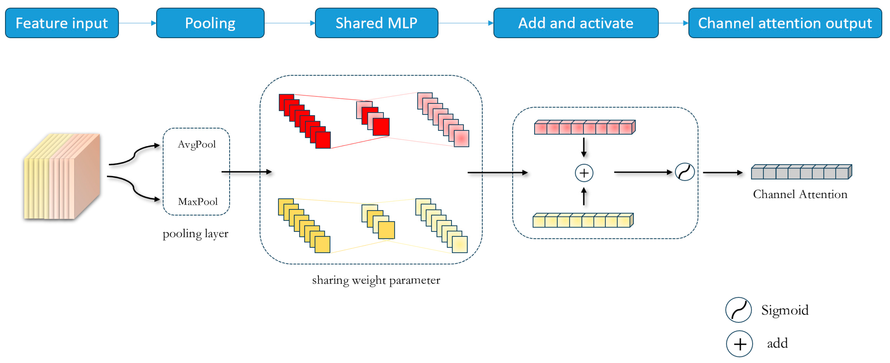
CAB is an important component of the CSAM module. It focuses on weighting attention given to the channel dimensions in the feature map [37,38]. The goal of the channel attention mechanism is to enhance the attention given to different channels by dynamically adjusting the weights between channels. This is crucial to improve the model’s ability to perceive different features in the image. The CAB module works as follows:
The steps of the CAB module are shown in Figure 3 below. Step 1: Firstly, the input feature map F i n is subjected to global average and maximum pooling operations, and the input information is compressed and downgraded to obtain two 1 × 1 average pooled features, F avg c , and maximum pooled features, F max c . Step 2: Then, they are fed into a weight-sharing two-layer neural network, MLP. Step 3: Finally, the MLP output features are subjected to an element-by-element summation operation, which is applied to the input feature map after activation by the Sigmoid function to generate the final Channel Attention Feature, M c . The above computational process is expressed as Equation (1), shown below:
M c ( F i n ) = σ ( M L P ( A v g P o o l ( F i n ) ) + M L P ( M a x P o o l ( F i n ) ) ) = σ ( W 1 ( W 0 ( F a v g c ) ) + W 1 ( W 0 ( F m a x c ) ) ) σ ( x ) = s i g m o i d ( x ) = 1 1 + e x
where σ ( ) is the sigmoid function and W 0 / W 1 represents the weights of the hidden/output layer. The parameters of W 0 and W 1 are shared in MLP.
Attention weights on the channel dimensions, indicating the contribution of different channels to the final feature representation, were generated by CAB, and these weights were applied to the original input feature map to generate features for the input spatial attention mechanism module. Channel-level feature tuning is achieved by weighting each channel’s features. This means that the model can better focus on the channel features that are important to the task at hand, improving the representation of semantic information.

2.2.2. SAB (Spatial Attention Block)

Unlike CAB, the SAB module focuses on the spatial dimension of the feature map. Its goal is to enhance the focus on different regions in the image by adjusting the weights of different spatial locations to improve the model’s perception of global contextual information. The SAB module works in Figure 4 as follows:
Step 1: First, the feature map output from the CAB module is used as the input of this module, F i n , and global maximum pooling and average pooling are done on the channel dimensions; then, these two results are used in a splicing operation. Step 2: Next, a 7 × 7 convolution kernel is chosen to perform a convolution operation on the splicing result, and the channel dimensions are reduced to 1. Step 3: Finally, after the Sigmoid activation function maps the weights between 0 and 1 to represent the order of importance of each position, these spatial attention weights are applied to the inputs to generate the feature map of the spatial channel attention mechanism, M s . The above computational process is expressed as Equation (2), shown below.
M s ( F i n ) = σ ( f 7 × 7 ( [ A v g P o o l ( F i n ) ; M a x P o o l ( F i n ) ] ) ) = σ ( f 7 × 7 ( F a v g s ; F m a x s ) )
where 7 × 7 is the kernel of convolution. This size performs better than others.
SAB generates attention weights in the spatial dimension through a series of convolutional operations and activation functions that indicate the contribution of different locations to the final feature representation. This means that the model can better focus on key regions in the image, thus improving the perception of global contextual information. The SAB module helps us to more accurately capture the contours and structure of objects in tasks such as semantic segmentation.

2.3. FFM (Feature Fusion Module)

The introduction of the FFM module [39,40,41] plays a key role in the process of feature fusion of information from different feature maps obtained from deeper and shallower layers when jump connections in the original network structure are involved. The FFM module allows us to efficiently fuse features of different scales and resolutions in order to capture the complex structure and irregular shapes of cloud shadows.
The steps of the FFM module are depicted in Figure 5. Step 1: Accept two feature maps with different resolutions from the encoder and decoder sections as input. Step 2: Perform a series of operations such as splicing, convolution, and so on, to fuse them into an enhanced hybrid feature map, which strengthens the representation of the hybrid features and makes them more suitable for subsequent processing. Step 3: Perform a global averaging of the hybrid feature map pooling to reduce the spatial dimension to 1 × 1 to obtain global channel statistics. Step 4: Introduce two consecutive 1 × 1 convolution operations via Relu and Sigmoid activation functions in order to enhance the nonlinearity and show the importance of each channel. Step 5: Multiply the channel attention weights with the element-by-element hybrid feature map obtained from Step 2 to perform the mul operation to obtain a weighted feature map. Step 6: Finally, the weighted feature map obtained from Step 5 is subjected to element-by-element add-sum operation with the hybrid feature map obtained from Step 2, to produce the final fused feature map. The above computational process is expressed as Equation (3), shown below.
F c o n v = C o n v ( C o n c a t ( F 1 , F 2 ) ) α = r e l u ( f 1 × 1 ( A v g P o o l ( F c o n v ) ) ) M F ( F 1 , F 2 ) = F c o n v + F c o n v σ ( f 1 × 1 ( α ) ) r e l u ( x ) = m a x ( 0 , x )
where F c o n v is the fusion of the input from shallow and deep layers and α represents the enhanced nonlinear result as an intermediate variable.
The FFM module is a well-designed feature fusion mechanism that effectively integrates feature maps from shallow and deep layers by means of utilizing channel complementarity, adaptively adjusting the weights of the channel features dynamically to better fuse information from different scales and semantic levels. This innovative fusion module offers an effective tool for our research and improves the performance of the capture and segmentation tasks of feature statistics.

2.4. Loss Function

The loss function is an important component in various segmentation network models based on deep learning [42]. It is used to measure the difference between the prediction and true values of the network and guide the model to make more accurate predictions. In the segmentation task, the reasonable selection, optimization, and innovation of the loss function can enhance the learning process of the model to achieve better segmentation results [43] as well as portability and application to other networks; thus, the study of the loss function selection is particularly important. The commonly used loss functions [44] are as follows:
1. Cross Entropy Loss Function
L = 1 N i = 1 N j = 1 N [ y i j log ( p i j ) + ( 1 y i j ) log ( 1 p i j ) ]
where N denotes the number of samples, and M denotes the number of categories. As the most commonly used loss function in image segmentation, which can be used in a large number of semantic segmentation tasks, the cross-entropy loss can help the network to correct categorization of the pixels after judging how good or bad the model is for the dataset.
2. Weighted Cross-Entropy Loss Function
L w = 1 N i = 1 N j = 1 N [ w j y i j log ( p i j ) + ( 1 y i j ) log ( 1 p i j ) ]
Despite being similar to the cross-entropy loss function, multiplying all positive samples by a coefficient for weighting allows the model to focus more on a smaller number of samples, thus mitigating the problem of the imbalanced number of categories.
3. Focal Loss
L F = 1 N i = 1 N j = 1 N [ ( 1 p i j ) y i j log ( p i j ) + p i j γ ( 1 y i j ) log ( 1 p i j ) ]
In addition to the imbalance in the number of samples from different categories, the problem of imbalance in the number of easily recognized samples and hard-to-recognize samples is often encountered, and the Focal Loss can help the network to better deal with the imbalance in the distribution of samples.
4. Dice Loss
L D = 1 2 X Y X + Y
where X Y is the intersection between samples X and Y, X represents the number of X samples, and Y stands for the number of Y samples.
Unlike the weighted cross-entropy loss function, the Dice Loss does not require category reweighting; it calculates the loss directly from the Dice coefficients, which can help the network better handle overlaps and boundaries between categories.
5. IOU Loss
L I = 1 X Y X Y
where X Y depicts the union between samples X and Y.
The IOU loss measures how similar the predicted segmentation results are to the true segmentation, and it helps to optimize the spatial consistency of the segmentation.
In summary, since the cloud shadows in the image are prone to overlap, and it is desired to distinguish the boundary between the two more accurately, L and LD are selected in this experiment for proper weighting to derive an innovative loss function applicable to the task of the dataset in this paper.
L o s s = α L + β L D
From Table 1, it is evident that the last row, which utilizes different weight proportions in the loss function weighted combination, achieves the best performance. This finding aligns with our initial conjecture. The Dice Loss effectively distinguishes between overlap regions and boundaries, aiding in completing the classification task more effectively. Moreover, continuous training is essential for further enhancing the model’s classification accuracy.

3. Experimental Analysis

3.1. Dataset

To further validate the generalization performance of the proposed model, we employed the GF1_WHU cloud shadow dataset created by Li et al. [45] as a generalization dataset. This dataset utilizes high-resolution GF-1 Wide Field of View (WFV) images with a spatial resolution of 16 m and covers four multispectral bands, spanning from visible to near-infrared spectral regions. The dataset consists of 108 GF-1 WFV 2a-level scene images, manually labeled by experts in remote sensing image interpretation at the SENDIMAGE laboratory of Wuhan University. These images encompass five main land cover types, including water, vegetation, urban areas, snow and ice, and barren land, representing different regions worldwide. During the model training process, we cropped the images to 256 × 256 pixels, removing black borders and unclear images, resulting in a total of 5428 images used for training and 1360 images for validation and testing, to evaluate the model’s training results, detection accuracy, and generalization performance. To illustrate the dataset effectively, we selected images from different scenes, as shown in Figure 6.
Each original image is captured by three channels of RGB: white represents clouds, gray represents cloud shadows, and black is the background. In addition, to prevent overfitting and to enhance the robustness of the model, we also augmented the dataset by randomly flipping, clipping, rotating, scaling, and panning the images as well as adding noise interference to the images.

3.2. Experimental Details

In this section, using the Legion Y740 laptop sourced from Lenovo in Beijing, China, we harness PyTorch 2.0 to train and test all models on its GeForce RTX 2080Ti graphics card based on the dataset introduced in the preceding dataset section. This comprehensive evaluation aims to assess the efficiency and accuracy of our proposed network model for cloud shadow segmentation. Through a series of ablation experiments and comparison experiments, we thoroughly evaluated our model from both qualitative and quantitative perspectives [46,47]. The quantitative metrics pixel accuracy (PA), precision (PC), recall (RC), mean intersection over union (MIoU), reconciliation average (F1), and frequency weighted intersection over union (FWIoU) are calculated as follows:
PA = TP + TN TP + TN + FP + FN
PC = TP TP + FP
RC = TP TP + FN
MIoU = TP TP + FP + FN
F 1 = 2 × PC × RC PC + RC
FWIoU = TP + FN TP + FP + TN + FN × TP TP + FP + FN
In Equations (10)–(15) above, TP represents true positives, which correspond to the number of pixels correctly identified as positive samples. Similarly, FP denotes false positives, indicating the number of pixels incorrectly classified as positive samples. TN refers to true negatives, representing the number of pixels accurately identified as negative samples. Lastly, FN signifies false negatives, indicating the number of pixels incorrectly classified as negative samples.
In this section, we provide a comprehensive evaluation of our proposed algorithm, verifying the efficiency and sophistication of our algorithm for the task of remote sensing image change detection through ablation experiments and comparison experiments. Our experiments are conducted on the GF1_WHU dataset, with an initial learning rate of 0.001. The number of samples used in each round is 4, the number of training samples is 5428, the number of training times is 150, and the quantitative metrics used are PR, RC, MIoU and F1.

3.3. Ablation Experiment

In conducting the ablation experiments, changes in the results are observed by censoring part of the network architecture and testing the effect of different modules on the whole model. Since UNet is the basic framework of our network, UNet is used as the starting point for comparison, where we use metrics such as PA, RC, F1, and MIoU to evaluate the performance of the model. As can be seen in Table 2 below, the combination of all components achieves the optimization of the model’s performance.
In order to enhance deep feature extraction, alleviate information loss resulting from constant down-sampling, and effectively capture multi-scale contextual information, as indicated by the ablation results of the deep feature sampling process, the CSAM Attention Mechanism Module proves beneficial for information recovery to capture detailed information. Additionally, the FFM module aids in better integrating contextual information, facilitating the fusion of features from different scales. Table 2 demonstrates a significant improvement in model performance following the introduction of these modules. Notably, the introduction of the Feature Fusion Module alone does not yield substantial improvements to the original model.

3.4. Comparison Experiment

In this experiment, the core of the cloud–shadow segmentation task is semantic segmentation, so our proposed network is compared with other semantic segmentation algorithms. PA, FWIoU, F1, and MIoU are selected as the evaluation metrics to comprehensively evaluate the performance of the model, as shown in Table 3.
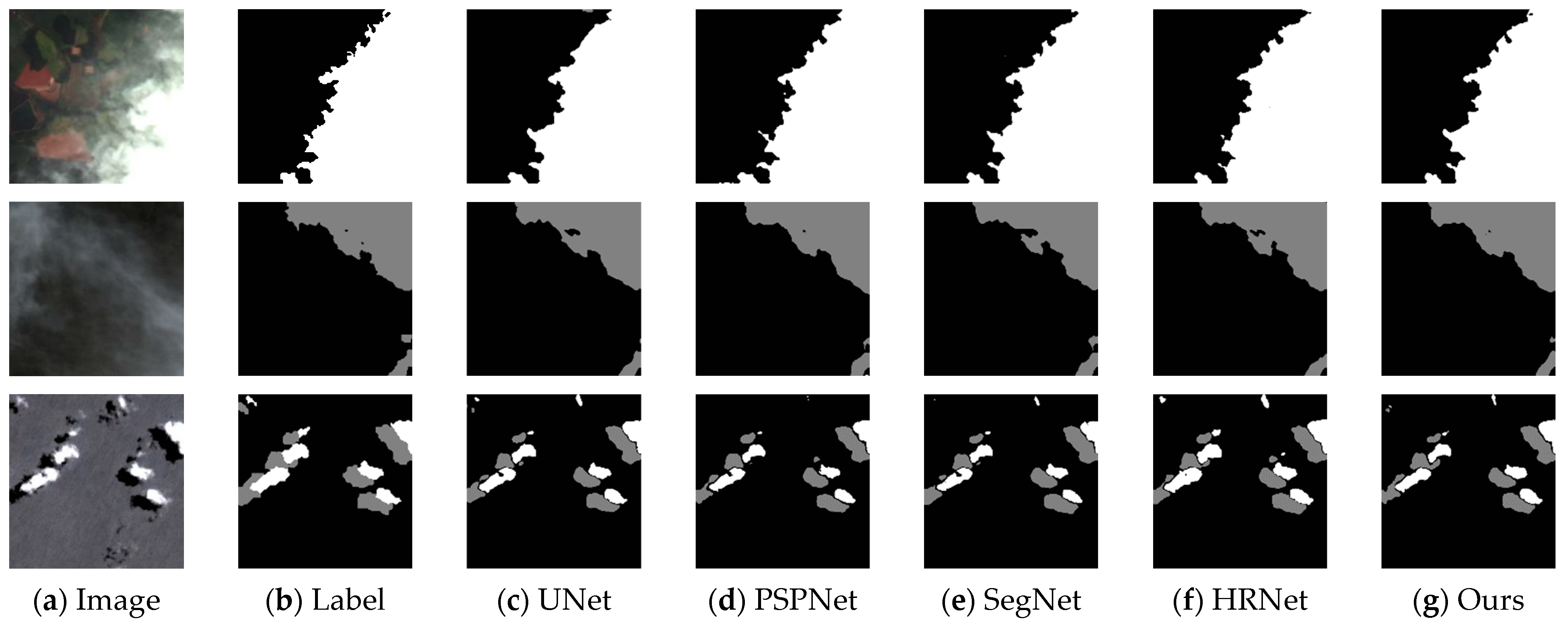
From the comparison results of different methods in the experimental setting in Table 3, it can be seen that our proposed algorithm outperforms the current traditional segmentation methods in all five metrics and is also basically better than the latest methods. Among all the networks considered, SegNet and FCN8 exhibit the poorest performance in terms of the metrics evaluated. While the metrics of the other models show improvement over successive iterations, they still fall short of the performance achieved by the models proposed in this paper. According to Table 3, we found that the above methods can achieve high-precision segmentation of cloud shadow datasets; to further visualize the effectiveness of our methods, Figure 7 shows the visualization experiment results of cloud shadow segmentation.
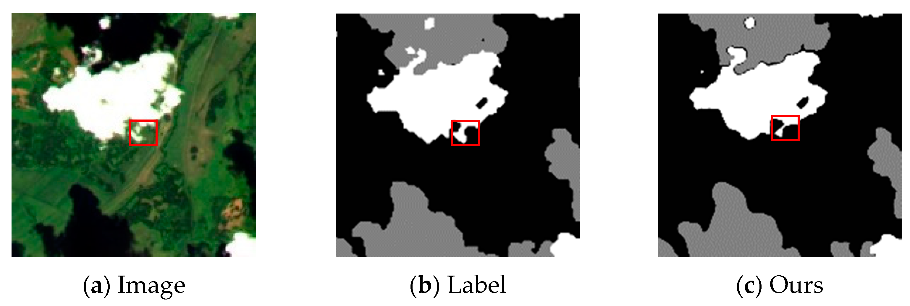
Figure 7 shows the visualization effect of different methods for image segmentation in the cloud shadow dataset. Eight examples are selected to demonstrate the segmentation effect. It can be observed that the proposed method is more accurate for cloud segmentation, especially in the segmentation of the edge region of the cloud. However, the performance is poor for cloud shadows and thin or unclear clouds. The segmentation effect of the Segnet model is relatively rough, the edge information is incompletely obtained, and too much information is lost in the feature extraction stage. It can be found from Figure 7 that it does not perform well at the boundary of the cloud and loses a lot of shape-striped feature information. When the texture is slightly complex, PSPNet cannot completely segment the boundary of clouds and cloud shadows. HRNet, on the other hand, slightly improves the effect compared to the above two models, with more delicate processing of the edges, but still has shortcomings compared to our model. UNet is a classic segmentation network known for its superior performance in training on smaller datasets and producing smoother segmentation edges. However, it still requires improvement in processing details. Our model addresses this limitation to some extent, effectively recognizing cloud and cloud shadow boundaries while enhancing detail processing. Nonetheless, further refinement is needed to effectively handle very low light or thin cloud bodies. In summary, from a qualitative point of view, our method performs better in different environments compared with other methods, which proves the importance and effectiveness of the model proposed in this paper.
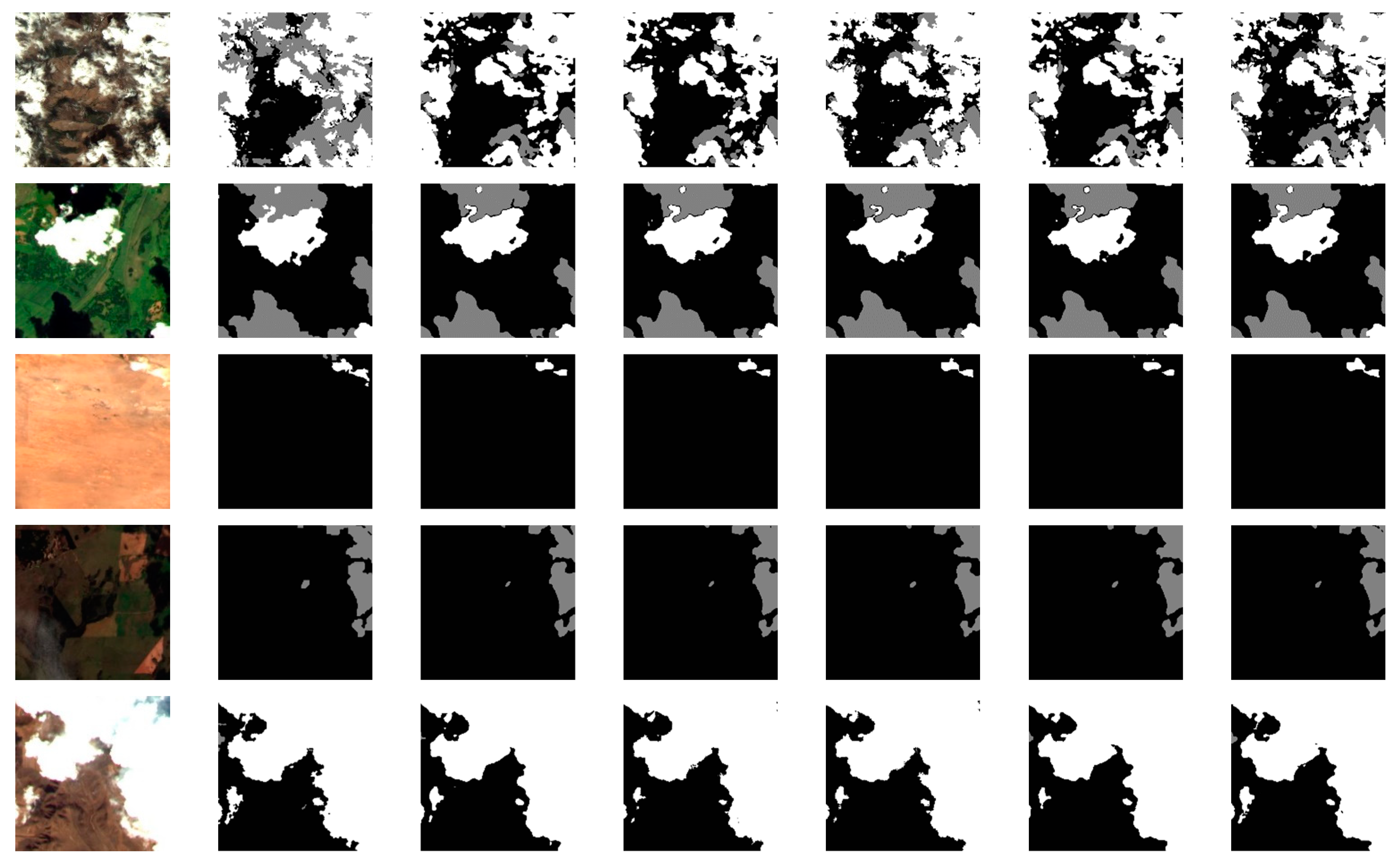
In order to better illustrate the model generalization and effectiveness of the model in the face of different environmental backgrounds, as shown in Figure 8 above, we chose vegetation, land, desert, barren, and snowy mountainous areas for model testing. For the images in the green vegetation environment in the first group, all are able to segment the general outline of the clouds well, but the details in the middle and background overlapping region are poor, and our model segments the edges of the clouds and the boundary well. In the second group, PSPNet, SegNet, and HRNet perform poorly for the shallow, scattered, and complex clouds, while UNet shows some improvement and recognizes the information of some thin clouds but still demonstrates a large deficiency compared to our model. By observing the third and fourth sets of images, it is not difficult to find that our model smoothly distinguishes the neighboring regions of clouds and cloud shadows and handles the edge information more naturally compared with other models. When confronted with remote sensing images containing significant noise interference, the performance of UNet, SegNet, and HRNet models is deemed insufficient. Instances of omission and misdetection, such as in the snowy mountain zones depicted in the comparative images, are observed. These models encounter challenges in accurately distinguishing between ice, snow, and clouds. Although the PSPNet segmentation effect offers some improvement, the texture features of the clouds are lost, and the boundary cannot be clearly reflected. None of the aforementioned models are suitable for the challenging task of cloud shadow segmentation across diverse and complex environments. In contrast, the algorithm proposed in this paper adeptly addresses cloud shadow segmentation in various situations and scenarios. By optimizing deeper features and leveraging the enhanced channel and feature fusion capabilities enabled by the spatial attention mechanism module, our algorithm effectively recovers high-definition remote sensing images.
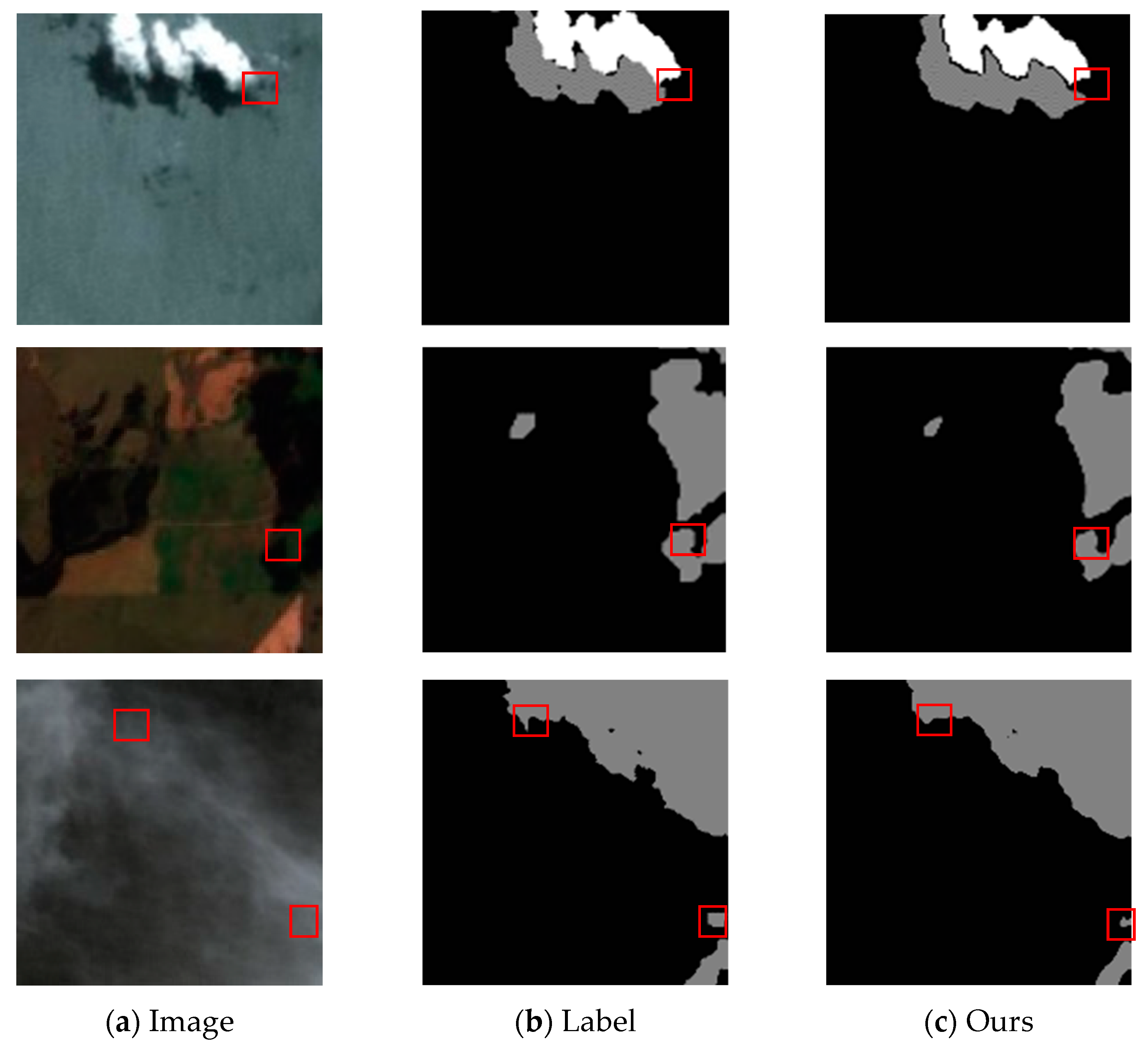
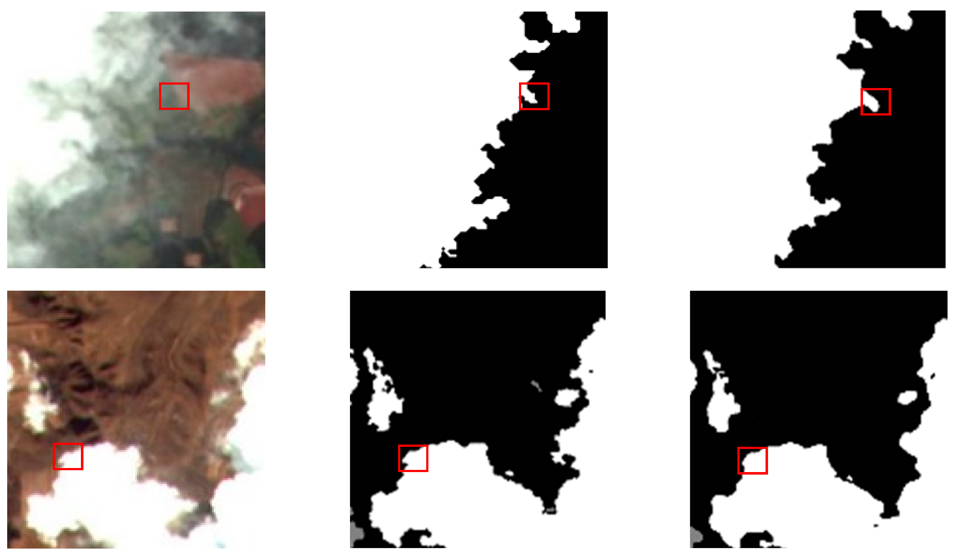
To further analyze our algorithm, we compared the segmentation results of different types of clouds, as shown in Figure 9 and Figure 10. It can be observed that our proposed model performs well in segmenting both thin and thick clouds, effectively delineating the overall contours of the clouds and shadows and clearly distinguishing them from the background. However, upon comparing the third row on the left with the second row on the right, it is evident that AFMUNet exhibits superior segmentation performance for thick clouds compared to thin clouds. Thick clouds only lose some fine texture details, while thin clouds tend to lose fragmented point cloud and shadow information during segmentation.

4. Conclusions

In remote sensing images, the accurate segmentation of cloud shadow regions is of great practical significance for practical tasks such as meteorological prediction, environmental monitoring, and natural disaster detection. In this paper, an attention mechanism feature aggregation algorithm is proposed for cloud shadow segmentation, fully leveraging the advantages of convolutional neural networks in deep learning. UNet is selected as the backbone network, an innovative loss function is employed, and two auxiliary modules, CSAM and FFM, are introduced. Our proposed model initiates constant down-sampling to extract high-level features. Adaptive improvement of sensory fields and selection of different channel operations are introduced during each up-sampling process to increase the resolution of feature maps, enabling the acquisition of rich contextual information. This facilitates the accurate fusion of low- and high-level information within each layer’s feature fusion module, ultimately restoring the classification and localization of high-resolution remote sensing images. Compared with previous deep learning and segmentation methods, our approach achieves significant improvement in accuracy in cloud shadow segmentation tasks. Experiments demonstrate the remarkable noise resistance and identification capabilities of this method. It accurately locates cloud shadows and segments fine cloud crevices in complex environments, while also producing smoother edge segmentation. Particularly noteworthy is its performance in the task of identifying thick clouds. However, there are still some shortcomings in cloud shadow segmentation: (1) under the influence of light, some inconspicuous cloud seams may be incorrectly segmented into other features and thus recognized as background; (2) refinement is still needed for the segmentation of thin clouds to capture the fragmented information of cloud shadows; (3) to be better adapted to practical applications, in the future, we also need to appropriately compress and simplify the model while maintaining the accuracy and reduce the segmentation result time to improve the training speed of the network. In the future, augmented learning can be implemented by incorporating a pre-training phase into the model, aiming to enhance segmentation accuracy and reduce training time. Additionally, efforts will be made to explore its application in other domains, including river segmentation and medical tumor segmentation.

Author Contributions

Conceptualization, Z.F.; methodology, W.D. and Z.F.; validation, W.D., Y.Y. and R.Y.; writing—original draft preparation, W.D. and J.L.; writing—review and editing, Y.Y.; visualization, J.L.; supervision, R.Y. All authors have read and agreed to the published version of the manuscript.

Funding

This research received no external funding.

Data Availability Statement

The data and the code of this study are available from the corresponding author upon request ([email protected]). The data are not publicly available due to restrictions (e.g., privacy, legal or ethical reasons).

Conflicts of Interest

The authors declare no conflicts of interest.

References

  1. Xiong, J.H.; Wu, H.; Gao, Y.; Cai, S.; Liang, D.; Yu, W.P. Ten years of remote sensing science: NSFC program fundings, progress, and challenges. Natl. Remote Sens. Bull. 2023, 27, 821–830. [Google Scholar] [CrossRef]
  2. Mahajan, S.; Fataniya, B. Cloud detection methodologies: Variants and development—A review. Complex Intell. Syst. 2020, 6, 251–261. [Google Scholar] [CrossRef]
  3. Saunders, R.W.; Kriebel, K.T. An improved method for detecting clear sky and cloudy radiances from AVHRR data. Int. J. Remote Sens. 1988, 9, 123–150. [Google Scholar] [CrossRef]
  4. Hutchinson, K.D.; Hardy, K.R. Threshold functions for automated cloud analyses of global meteorological satellite imagery. Int. J. Remote Sens. 1995, 16, 3665–3680. [Google Scholar] [CrossRef]
  5. Xiong, Q.; Wang, Y.; Liu, D.; Ye, S.; Du, Z.; Liu, W.; Huang, J.; Su, W.; Zhu, D.; Yao, X.; et al. A cloud detection approach based on hybrid multispectral features with dynamic thresholds for GF-1 remote sensing images. Remote Sens. 2020, 12, 450. [Google Scholar] [CrossRef]
  6. Derrien, M.; Farki, B.; Harang, L.; LeGléau, H.; Noyalet, A.; Pochic, D.; Sairouni, A. Automatic cloud detection applied to NOAA-11/AVHRR imagery. Remote Sens. Environ. 1993, 46, 246–267. [Google Scholar] [CrossRef]
  7. Clothiaux, E.E.; Miller, M.A.; Albrecht, B.A.; Ackerman, T.P.; Verlinde, J.; Babb, D.M.; Peters, R.M.; Syrett, W.J. An evaluation of a 94-GHz radar for remote sensing of cloud properties. J. Atmos. Ocean. Technol. 1995, 12, 201–229. [Google Scholar] [CrossRef]
  8. Danda, S.; Challa, A.; Sagar BS, D. A morphology-based approach for cloud detection. In Proceedings of the 2016 IEEE International Geoscience and Remote Sensing Symposium (IGARSS), Beijing, China, 10–15 July 2016; pp. 80–83. [Google Scholar] [CrossRef]
  9. Liu, X.; Shen, J.P.; Huang, Y. Cloud automatic detection in high-resolution satellite images based on morphological features. In Proceedings of the Eleventh International Conference on Graphics and Image Processing (ICGIP 2019), Hangzhou, China, 12–14 October 2019; SPIE: Bellingham, WA, USA, 2020; Volume 11373, pp. 159–166. [Google Scholar] [CrossRef]
  10. Tom, V.T.; Peli, T.; Leung, M.; Bondaryk, J.E. Morphology-based algorithm for point target detection in infrared backgrounds. In Proceedings of the Signal and Data Processing of Small Targets 1993, Orlando, FL, USA, 12–14 April 1993; SPIE: Bellingham, WA, USA, 1993; Volume 1954, pp. 2–11. [Google Scholar] [CrossRef]
  11. Amato, U.; Antoniadis, A.; Cuomo, V.; Cutillo, L.; Franzese, M.; Murino, L.; Serio, C. Statistical cloud detection from SEVIRI multispectral images. Remote Sens. Environ. 2008, 112, 750–766. [Google Scholar] [CrossRef]
  12. Wylie, D.; Jackson, D.L.; Menzel, W.P.; Bates, J.J. Trends in global cloud cover in two decades of HIRS observations. J. Clim. 2005, 18, 3021–3031. [Google Scholar] [CrossRef]
  13. Abuhussein, M.; Robinson, A. Obscurant Segmentation in Long Wave Infrared Images Using GLCM Textures. J. Imaging 2022, 8, 266. [Google Scholar] [CrossRef]
  14. Shao, L.; He, J.; Lu, X.; Hei, B.; Qu, J.; Liu, W. Aircraft Skin Damage Detection and Assessment from UAV Images Using GLCM and Cloud Model. IEEE Trans. Intell. Transp. Syst. 2023, 25, 3191–3200. [Google Scholar] [CrossRef]
  15. Reiter, P. Cloud Detection Through Wavelet Transforms in Machine Learning and Deep Learning. arXiv 2020, arXiv:2007.13678. [Google Scholar]
  16. Gupta, R.; Panchal, P. Cloud detection and its discrimination using Discrete Wavelet Transform in the satellite images. In Proceedings of the 2015 International Conference on Communications and Signal Processing (ICCSP), Melmaruvathur, India, 2–4 April 2015; pp. 1213–1217. [Google Scholar] [CrossRef]
  17. Changhui, Y.; Yuan, Y.; Minjing, M.; Menglu, Z. Cloud detection method based on feature extraction in remote sensing images. Int. Arch. Photogramm. Remote Sens. Spat. Inf. Sci. 2013, 40, 173–177. [Google Scholar] [CrossRef]
  18. Surya, S.R.; Rahiman, M.A. Cloud detection from satellite images based on Haar wavelet and clustering. In Proceedings of the 2017 International Conference on Nextgen Electronic Technologies: Silicon to Software (ICNETS2), Chennai, India, 23–25 March 2017; pp. 163–167. [Google Scholar] [CrossRef]
  19. Li, P.; Dong, L.; Xiao, H.; Xu, M. A cloud image detection method based on SVM vector machine. Neurocomputing 2015, 169, 34–42. [Google Scholar] [CrossRef]
  20. Ishida, H.; Oishi, Y.; Morita, K.; Moriwaki, K.; Nakajima, T.Y. Development of a support vector machine based cloud detection method for MODIS with the adjustability to various conditions. Remote Sens. Environ. 2018, 205, 390–407. [Google Scholar] [CrossRef]
  21. Fu, H.; Shen, Y.; Liu, J.; He, G.; Chen, J.; Liu, P.; Qian, J.; Li, J. Cloud detection for FY meteorology satellite based on ensemble thresholds and random forests approach. Remote Sens. 2018, 11, 44. [Google Scholar] [CrossRef]
  22. Jin, Z.; Zhang, L.; Liu, S.; Yi, F. Cloud detection and cloud phase retrieval based on BP neural network. Opt. Optoelectron. Technol. 2016, 14, 74–77. [Google Scholar]
  23. Long, J.; Shelhamer, E.; Darrell, T. Fully convolutional networks for semantic segmentation. In Proceedings of the IEEE Conference on Computer Vision and Pattern Recognition, San Juan, PR, USA, 17–19 June 2015; pp. 3431–3440. [Google Scholar]
  24. Mohajerani, S.; Krammer, T.A.; Saeedi, P. Cloud detection algorithm for remote sensing images using fully convolutional neural networks. arXiv 2018, arXiv:1810.05782. [Google Scholar]
  25. Badrinarayanan, V.; Kendall, A.; Cipolla, R. Segnet: A deep convolutional encoder-decoder architecture for image segmentation. IEEE Trans. Pattern Anal. Mach. Intell. 2017, 39, 2481–2495. [Google Scholar] [CrossRef] [PubMed]
  26. Lu, J.; Wang, Y.; Zhu, Y.; Ji, X.; Xing, T.; Li, W.; Zomaya, A.Y. P_SegNet and NP_SegNet: New neural network architectures for cloud recognition of remote sensing images. IEEE Access 2019, 7, 87323–87333. [Google Scholar] [CrossRef]
  27. Chen, L.-C.; Papandreou, G.; Kokkinos, I.; Murphy, K.; Yuille, A.L. Deeplab: Semantic image segmentation with deep convolutional nets, atrous convolution, and fully connected crfs. IEEE Trans. Pattern Anal. Mach. Intell. 2017, 40, 834–848. [Google Scholar] [CrossRef] [PubMed]
  28. Ronneberger, O.; Fischer, P.; Brox, T. U-net: Convolutional networks for biomedical image segmentation. In Proceedings of the Medical Image Computing and Computer-Assisted Intervention–MICCAI 2015: 18th International Conference, Munich, Germany, 5–9 October 2015; Proceedings, Part III 18. Springer International Publishing: Berlin/Heidelberg, Germany, 2015; pp. 234–241. [Google Scholar] [CrossRef]
  29. Zhao, H.; Shi, J.; Qi, X.; Wang, X.; Jia, J. Pyramid scene parsing network. In Proceedings of the IEEE Conference on Computer Vision and Pattern Recognition, Honolulu, HI, USA, 21–26 July 2017; pp. 2881–2890. [Google Scholar]
  30. Zhang, Z.; Yang, S.; Liu, S.; Cao, X.; Durrani, T.S. Ground-based remote sensing cloud detection using dual pyramid network and encoder–decoder constraint. IEEE Trans. Geosci. Remote Sens. 2022, 60, 1–10. [Google Scholar] [CrossRef]
  31. Tsotsos, J.K. Analyzing vision at the complexity level. Behav. Brain Sci. 1990, 13, 423–445. [Google Scholar] [CrossRef]
  32. Ding, L.; Xia, M.; Lin, H.; Hu, K. Multi-level attention interactive network for cloud and snow detection segmentation. Remote Sens. 2023, 16, 112. [Google Scholar] [CrossRef]
  33. Sutskever, I.; Vinyals, O.; Le, Q.V. Sequence to sequence learning with neural networks. Adv. Neural Inf. Process. Syst. 2014, 27. [Google Scholar] [CrossRef]
  34. Hu, K.; Li, Y.; Zhang, S.; Wu, J.; Gong, S.; Jiang, S.; Weng, L. FedMMD: A Federated weighting algorithm considering Non-IID and Local Model Deviation. Expert Syst. Appl. 2024, 237, 121463. [Google Scholar] [CrossRef]
  35. Guo, M.-H.; Xu, T.-X.; Liu, J.-J.; Liu, Z.-N.; Jiang, P.-T.; Mu, T.-J.; Zhang, S.-H.; Martin, R.R.; Cheng, M.-M.; Hu, S.-M. Attention mechanisms in computer vision: A survey. Comput. Vis. Media 2022, 8, 331–368. [Google Scholar] [CrossRef]
  36. Liu, Y.; Shao, Z.; Hoffmann, N. Global attention mechanism: Retain information to enhance channel-spatial interactions. arXiv 2021, arXiv:2112.05561. [Google Scholar]
  37. Hu, K.; Zhang, D.; Xia, M.; Qian, M.; Chen, B. LCDNet: Light-weighted cloud detection network for high-resolution remote sensing images. IEEE J. Sel. Top. Appl. Earth Obs. Remote Sens. 2022, 15, 4809–4823. [Google Scholar] [CrossRef]
  38. Ji, H.; Xia, M.; Zhang, D.; Lin, H. Multi-supervised feature fusion attention network for clouds and shadows detection. ISPRS Int. J. Geo-Inf. 2023, 12, 247. [Google Scholar] [CrossRef]
  39. Yu, C.; Wang, J.; Peng, C.; Gao, C.; Yu, G.; Sang, N. Bisenet: Bilateral segmentation network for real-time semantic segmentation. In Proceedings of the European Conference on Computer Vision (ECCV), Munich, Germany, 8–14 September 2018; pp. 325–341. [Google Scholar]
  40. Hu, K.; Zhang, E.; Dai, X.; Xia, M.; Zhou, F.; Weng, L.; Lin, H. MCSGNet: A Encoder–Decoder Architecture Network for Land Cover Classification. Remote Sens. 2023, 15, 2810. [Google Scholar] [CrossRef]
  41. Wang, Z.; Xia, M.; Weng, L.; Hu, K.; Lin, H. Dual encoder-decoder network for land cover segmentation of remote sensing image. IEEE J. Sel. Top. Appl. Earth Obs. Remote Sens. 2023, 17, 2372–2385. [Google Scholar] [CrossRef]
  42. Wang, Q.; Ma, Y.; Zhao, K.; Tian, Y. A comprehensive survey of loss functions in machine learning. Ann. Data Sci. 2020, 9, 187–212. [Google Scholar] [CrossRef]
  43. Hu, K.; Weng, C.; Shen, C.; Wang, T.; Weng, L.; Xia, M. A multi-stage underwater image aesthetic enhancement algorithm based on a generative adversarial network. Eng. Appl. Artif. Intell. 2023, 123, 106196. [Google Scholar] [CrossRef]
  44. Ma, J. Segmentation loss odyssey. arXiv 2020, arXiv:2005.13449. [Google Scholar] [CrossRef]
  45. Li, Z.; Shen, H.; Li, H.; Xia, G.; Gamba, P.; Zhang, L. Multi-feature combined cloud and cloud shadow detection in GaoFen-1 wide field of view imagery. Remote Sens. Environ. 2017, 191, 342–358. [Google Scholar] [CrossRef]
  46. Ren, H.; Xia, M.; Weng, L.; Hu, K.; Lin, H. Dual Attention-Guided Multiscale Feature Aggregation Network for Remote Sensing Image Change Detection. IEEE J. Sel. Top. Appl. Earth Obs. Remote Sens. 2024, 17, 4899–4916. [Google Scholar] [CrossRef]
  47. Jiang, S.; Dong, R.; Wang, J.; Xia, M. Credit card fraud detection based on unsupervised attentional anomaly detection network. Systems 2023, 11, 305. [Google Scholar] [CrossRef]
  48. Fu, J.; Liu, J.; Tian, H.; Li, Y.; Bao, Y.; Fang, Z.; Lu, H. Dual attention network for scene segmentation. In Proceedings of the IEEE/CVF Conference on Computer Vision and Pattern Recognition, Long Beach, CA, USA, 15–20 June 2019; pp. 3146–3154. [Google Scholar]
  49. Yu, C.; Gao, C.; Wang, J.; Yu, G.; Shen, C.; Sang, N. Bisenet v2: Bilateral network with guided aggregation for real-time semantic segmentation. Int. J. Comput. Vis. 2021, 129, 3051–3068. [Google Scholar] [CrossRef]
  50. Wang, J.; Sun, K.; Cheng, T.; Jiang, B.; Deng, C.; Zhao, Y.; Liu, D.; Mu, Y.; Tan, M.; Wang, X.; et al. Deep high-resolution representation learning for visual recognition. IEEE Trans. Pattern Anal. Mach. Intell. 2020, 43, 3349–3364. [Google Scholar] [CrossRef]
  51. Qu, Y.; Xia, M.; Zhang, Y. Strip pooling channel spatial attention network for the segmentation of cloud and cloud shadow. Comput. Geosci. 2021, 157, 104940. [Google Scholar] [CrossRef]
  52. Hu, K.; Zhang, D.; Xia, M. CDUNet: Cloud detection UNet for remote sensing imagery. Remote Sens. 2021, 13, 4533. [Google Scholar] [CrossRef]
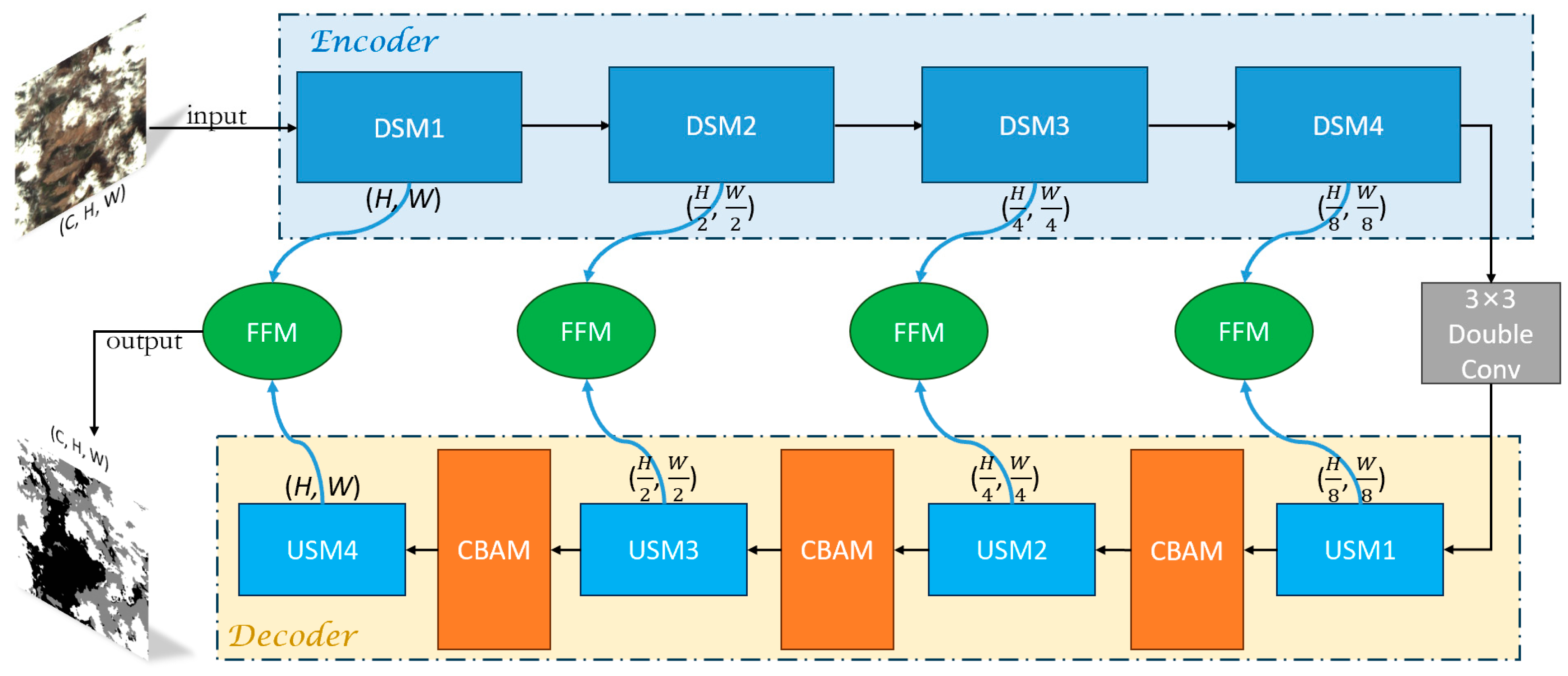
Figure 1. Attention mechanism feature fusion network framework based on U-shaped structure.
Remotesensing 16 01574 g001
Figure 2. Channel space attention mechanism module.
Remotesensing 16 01574 g002
Figure 3. Channel attention block.
Remotesensing 16 01574 g003
Figure 4. Spatial attention block.
Remotesensing 16 01574 g004
Figure 5. Feature fusion module.
Remotesensing 16 01574 g005
Figure 6. Examples from GF1_WHU Wuhan University cloud shadow dataset: (a) water; (b) vegetation; (c) snow; (d) ice; (e) barren.
Remotesensing 16 01574 g006
Figure 7. Comparison of visualization results for different models: (a) the original image; (b) the corresponding label; (c) the prediction of UNet; (d) the prediction of PSPNet; (e) the prediction of SegNet; (f) the prediction of HRNet; (g) the prediction of the proposed AFMUNet.
Remotesensing 16 01574 g007aRemotesensing 16 01574 g007b
Figure 8. Fine comparison of different models in different contexts: (a) the original image; (b) the corresponding label; (c) the prediction of UNet; (d) the prediction of PSPNet; (e) the prediction of SegNet; (f) the prediction of HRNet; (g) the prediction of the proposed AFMUNet. (Red boxes indicate better segmentation results, while green boxes segment poorer results).
Remotesensing 16 01574 g008
Figure 9. Results of thin cloud segmentation: (a) the original image; (b) the corresponding label; (c) the prediction of the proposed AFMUNet. (Red boxes indicate noteworthy edge details of the result).
Remotesensing 16 01574 g009
Figure 10. Results of thick cloud segmentation: (a) the original image; (b) the corresponding label; (c) the prediction of the proposed AFMUNet. (Red boxes indicate better segmented edge details).
Remotesensing 16 01574 g010aRemotesensing 16 01574 g010b
Table 1. Effect of different combinations of weight coefficients on segmentation results.
α β MPA (%)MIoU (%)
0.20.865.9358.69
0.30.771.9758.79
0.40.677.0465.77
0.50.576.5965.07
0.60.481.8678.22
0.70.387.3286.30
0.80.296.8893.02
Table 2. Performance comparison of different combinations of modules in the model.
MethodPA (%)RC (%)PC (%)F1 (%)MIoU (%)
UNet95.2789.7293.2492.0391.30
UNet + CSAM96.48 (↑)94.3295.0293.4192.89
UNet + FFM95.3294.8393.6291.8291.33
UNet + CSAM + FFM96.93 (↑)95.8294.9793.7593.21
UNet + CSAM + FFM + Loss
AFMUNet (Ours)
97.1296.0393.2193.9093.42
The arrow means this kind of combination improves the performance of model. The bold indicates the highest value in the column.
Table 3. Results on GF1_WHU dataset testing set.
MethodPA (%)MPA (%)MIoU (%)F1 (%)FWIoU (%)
SegNet94.8093.9088.2890.7790.16
UNet96.3395.4991.3293.2192.80
FCN8s95.2094.8490.5892.9292.36
PSPNet96.5195.7891.7693.8993.31
DANet [48]94.8294.1389.2591.7091.32
DeepLab V3Plus96.2795.4291.1893.1192.56
BiseNet V2 [49]95.7694.8590.2792.3491.87
HRNet [50]96.8795.7392.0293.9393.40
SP_CSANet [51]97.3396.0191.3493.1292.63
CDUNet [52]97.2196.5393.3395.0394.58
AFMUNet (Ours)97.4096.6293.2895.1094.43
Disclaimer/Publisher’s Note: The statements, opinions and data contained in all publications are solely those of the individual author(s) and contributor(s) and not of MDPI and/or the editor(s). MDPI and/or the editor(s) disclaim responsibility for any injury to people or property resulting from any ideas, methods, instructions or products referred to in the content.