Abstract
Crop yield forecasting during an ongoing season is crucial to ensure food security and commodity markets. For this reason, here, a scalable approach to forecast corn yields at the field-level using machine learning and satellite imagery from Sentinel-2 and Landsat missions is proposed. The model, evaluated on 1319 corn fields in the U.S. Corn Belt from 2017 to 2022, integrates biophysical parameters from Sentinel-2, Land Surface Temperature (LST) from Landsat, and agroclimatic data from ERA5 reanalysis dataset. Resampling the time series over thermal time significantly enhances predictive performance. The addition of LST to our model further improves in-season yield forecasting, through its capacity to detect early drought, which is not immediately visible to optical sensors such as the Sentinel-2. Finally, we propose a new two-stage machine learning strategy to mitigate early season partially available data. It consists in extending the current time series on the basis of complete historical data and adapting the model inference according to the crop progress.
1. Introduction
Monitoring and predicting crop phenology, growth, and yield is crucial for global food security, market dynamics, policy making, and decision making [1]. Accurate early season estimations of crop yield provides farmers with an estimate of their production, enabling them to assess risks, determine insurance premiums, and evaluate input costs [2]. In addition to supporting individual farmers, it contributes to a broader understanding of the complex interplay between environmental factors and management practices in agriculture [3]. This understanding facilitates the development of more effective and flexible within-season management strategies [4,5] and enables the anticipation of market demand by forecasting supply [6].
Traditional methods such as manual sampling and field campaigns are labor-intensive, and provide limited insights into the spatial variability of crop yield. These limitations have led to the development of alternative approaches for estimating yields during the growing season [7]. Using advanced technologies and data-driven methods, these yield forecasts not only reduce the work and time spent on measurements, but also improve the spatial coverage and accuracy of the obtained information [1]. In recent years, there have been remarkable advances in yield forecasting methods that use Earth Observation (EO) data, satellite remote sensing imagery, acquired via modern missions. This technology has become a valuable source of information for monitoring agricultural practices. By exploiting EO data, within-season (or early season) crop yield forecasts can now be provided, enabling farmers and stakeholders to make informed decisions leading to optimal production [8]. This advancement primarily stems from the availability of near real-time data (NRT) EO datasets from open sources with optical instruments on satellites like SPOT, MODIS, PROBA-V, and Landsat which have played a crucial role in such operational crop monitoring [9]. These instruments offer several benefits, including daily revisit cycles, global coverage, long-term data archives, and low- or no-cost accessibility. However, there is a quest for generic time series analysis methods for crop mapping and monitoring that can be deployed at a large scale, taking advantage of the global coverage, with high spatial and temporal resolution, provided by modern Earth observation missions.
The launch of Sentinel-2A (S2A) in late 2015 and Sentinel-2B (S2B) in early 2017 has significantly enhanced crop monitoring capabilities. S2A provides a 10-day revisit time period over Europe and Africa, and 20 days elsewhere, while S2B ensures a 5-day revisit time period worldwide since February 2018 [10]. This unprecedented revisit time is particularly suitable for in-season crop monitoring. Unlike previous Earth Observation (EO) missions, Sentinel-2 enables the derivation of red-edge-based vegetation indices, which exhibit stronger correlations with agronomic parameters compared to red-based indices [11]. The combination of Copernicus’ free and open access policy with the high resolution of Sentinel-2 images allows for the construction of dense and consistent time series throughout the crop growth cycle in most regions of the world [12]. Consequently, Sentinel-2 satellite imagery, with its spectral bands (visible, near infrared, red-edge, and short-wave infrared) and spatial resolutions (10 m, 20 m, and 60 m), has been successfully exploited in recent years for modeling crop grain yield at field and within-field scales [1,13,14].
Before the advent of Sentinel-2, Landsat satellite data played a crucial role in accurately mapping crop types and predicting yields at the field level in agricultural landscapes, worldwide [15]. With a temporal resolution of 8 days, Landsat 7 and 8 (before 2022) and Landsat 8 and 9 (after 2022) images offer a tangible advantage in crop monitoring when coupled with Sentinel-2, fully enriching the latter with the information provided by Landsat thermal bands [16]. The Landsat missions are currently the only constellation equipped with thermal bands, provided at an adequate spatial resolution (100 meters), for precise monitoring at the scale of individual fields. Land surface temperature (LST), derived from these thermal bands, is used to monitor heat stress and drought, which can explain some of the variability in yields between years [2,17]. Indeed, relying solely on early season optical remote sensing data can make it difficult to detect the onset of drought, which mainly captures information on the upper canopy. This is because drought symptoms tend to appear earlier in the lower leaves, potentially underestimating the negative effects of drought on yield [18]. At the county scale, studies have shown a negative correlation between MODIS diurnal LST and mid-summer corn yield forecasts [2]. However, in satellite-based agricultural modeling, studies mainly focus on vegetation indices in the visible and near-infrared part of the electromagnetic spectrum, and potential data related to Land Surface Temperature are often neglected [19]. We therefore considered it important to evaluate LST as an input variable in our task of early season crop yield prediction.
When it comes to yield estimation methods, mechanistic crop growth models are the standard choice, as they are designed and calibrated to simulate yield formation processes using soil information, climate and farm management practices. They enable crop yields to be predicted at any time and in any place [5], but the need for extensive (and often costly) data on field-specific biotic and abiotic factors limits the large-scale deployment of these approaches over the ongoing season [2,15,20]. In contrast, machine learning (ML) algorithms can handle complex relationships between predictors and the target variables, leading to their increased use in the agriculture domain [21,22,23].
A key limitation of ML methods for crop yield prediction is their dependence on data acquired under specific local conditions, which may result in inaccurate forecasts when confronted with data acquired under unseen conditions not included in the model’s training data [24]. This may be partly explained by possible differences in crop progress and climate/environmental condition changes from season to season, or from location to location, where these seasonal changes in phenology are primarily influenced by temperature and water regimes [25]. To face such generalization issues affecting modern ML approaches, in the context of yield prediction, a possible solution is to resample remote sensing satellite image data over periods calculated over thermal time, i.e., the number of growing degrees–days accumulated from the sowing date, rather than calendar time [26], with the aim of mitigating possible shifts in crop phenology at a given date, due to different temperature regimes.
The research is founded upon a cut-off date of mid-August, approximately two months prior to the corn harvest. This timeframe corresponds to the initial stages of maize reproduction, including heading and pollination, with regional variations influenced by planting dates [27]. At this juncture, grain filling commences, during which kernel size begins to develop, while the kernel count has already been established in prior stages. Consequently, pre-stage crop conditions and weather patterns can significantly impact yield potential. The objective of this study is to contribute to the comprehension of utilizing remote sensing data for estimating in-season corn yield through the application of machine learning methodologies.
From a methodological point of view, our approach is based on a real-life deployment scenario of a machine learning framework. In this framework, a model is trained using reference data collected during previous seasons. With regard to the selection and processing of predictors, our methodology includes (1) the incorporation of thermal time to account for the various phenological advances of crops, which depend on temperature regimes rather than a fixed number of days, (2) the integration of Land Surface Temperature (LST) and agroclimatic stress indicators to address the limitation of optical imagery which does not reach its full potential during the growing season, and (3) the exploitation of comprehensive historical information covering the whole season to improve predictions for the current early season forecasting task.
In this study, a multi-year proprietary dataset is utilized, comprising data from 1319 corn production fields predominantly situated across 29 counties within the U.S. Corn Belt spanning the years 2017 to 2022. The dataset includes the average yield of each field, and for evaluation purposes, each year is assessed independently, with the remaining years serving as the training dataset for the model.
2. Materials
2.1. Corn Yield Dataset
The research site is primarily located in the U.S. Corn Belt, the largest corn-producing states in the United States. A total of 1319 corn fields are available, of which 849 fields were located in Nebraska, 423 in Iowa, 29 in Illinois, and 21 in Wisconsin.
The yield dataset utilized in this study, provided by Syngenta (Syngenta is an international leading science-based agtech company https://www.syngenta.com/en/company (accessed on 10 October 2023)), comprises direct measurements of corn yield obtained from seed production fields. These fields are utilized for crossbreeding two corn varieties, consisting of male and female plants. During harvesting, only the female plants are collected, as the male plants are sterile. Therefore, the yield data is obtained solely from the harvested female acres. The measurements are derived from the weight of harvested corn, adjusted for moisture content to 15.5% and measured in green bushels per female acre (GB/FA).
The size of the fields ranged from 3.9 to 276 female acres. Female parental lines were on average planted on day of the year 137 (±9.3) and harvested on day 263 (±9.8), and the average length of the growing was 126 days (±9.1). The distribution of yield across different years is depicted in Figure 1b. In Figure 2, the average yield data at the county level across all historical records is depicted to assess spatial heterogeneity. For data confidentiality, the yield values were scaled between 0 and 1 using min–max normalization across all fields.

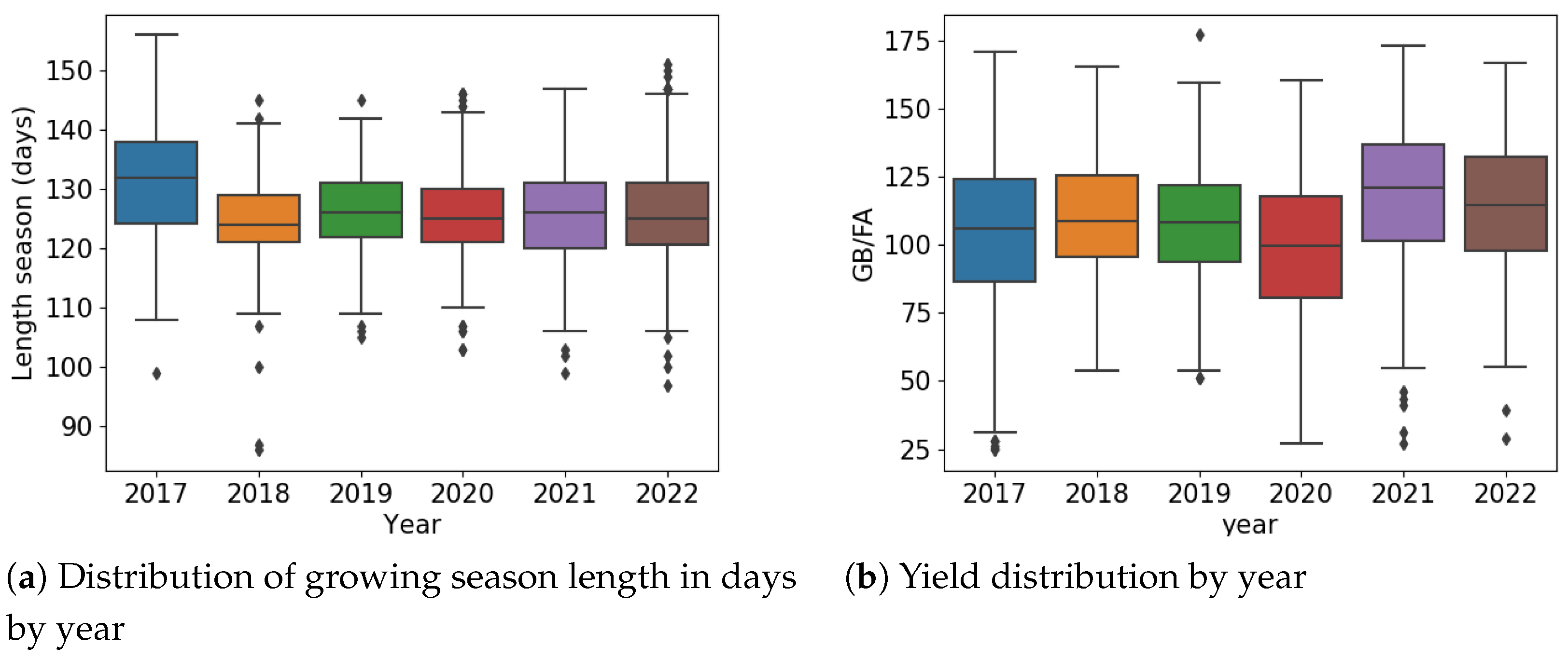
Figure 1.
The boxplots illustrate the strong disparities in distribution observed between years, indicating significant heterogeneity in our data. Seasonal durations (a) ranged from 110 to 150 days from sowing to harvest, with a median duration of around 125 days. As for crop yields (b), they ranged from 25 to 175 bushels per acre, highlighting significant year-to-year variability. For example, the median yield in 2020 was 100 bushels, while it was 125 bushels in 2021. All data points, including those outside the boxplot whiskers, are retained in this study as they represent genuine measurements.
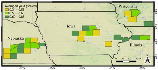
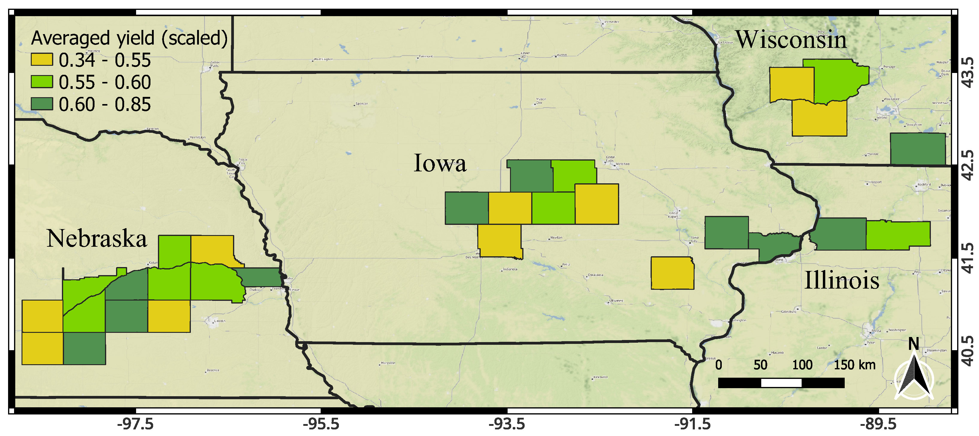
Figure 2.
Seed production fields are spatially distributed over 29 counties in eastern Nebraska, Iowa, Illinois and Wisconsin.
In this study, the machine learning model utilized some in situ features, namely the corn cultivar duration (FAO maturity groups) of the female parental lines, whether the field was irrigated or not, and the geographic coordinates (expressed in decimal degrees and rounded off by a factor of 1), to integrate information from the local environment and the farming practices.
2.2. Satellite Data
2.2.1. Acquisition
Raw data from the Sentinel-2 and Landsat missions were collected using the open-source eo-learn Python library developed by Sinergise (https://github.com/sentinel-hub/eo-learn, accessed on 10 October 2023). This framework provides a Python client for downloading and pre-processing level 2A atmosphere-corrected data from the SentinelHub cloud platform. The raw band pixels were resampled to a 10-meter reference grid using nearest neighbor interpolation. Within each image, pixels identified as saturated, shaded, or cloudy using the scene classification map (SLC) obtained from sen2cor [28] were excluded from subsequent analyses. Then, the percentage of pixels previously identified as invalid relative to the total number of pixels within the field bounding box was calculated. Only acquisition dates with more than 50% valid pixels were retained for the analysis.
To ensure the model receives adequate data for accurate predictions during the growing season, specific rules were established to select observations from the whole set of data. More precisely, a minimum of four Sentinel-2 and Landsat 7/8/9 images was required between the beginning of May and the end of July, with at least one image needed in the first half of August. Challenges arose from limited image availability, particularly in 2017, where only Sentinel-2A was accessible, averaging eight images between May and September (Table 1). Additionally, in 2019, a technical issue with the Landsat-8 satellite temporarily reduced the number of exploitable Landsat images. Termed as a “degraded image quality” event, this issue occurred in May 2019, resulting in a decreased number of exploitable images for that season.

Table 1.
Summary statistics in-situ data. The values reported are mean ± standard deviation.
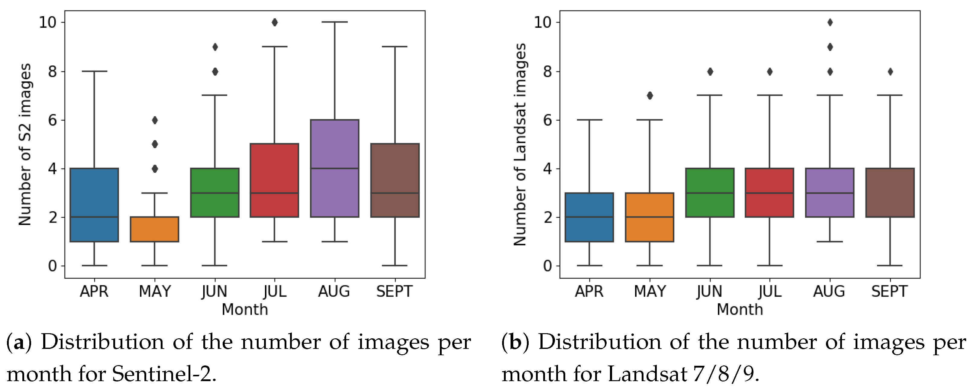
Figure 3a,b depict the distribution of the number of Sentinel-2 and Landsat 7/8/9 images from April to September, aggregated over all considered years. August emerges with the highest number of associated images, with a median of four Sentinel-2 images and three Landsat images. However, in May, a maximum of only two available Sentinel-2 images was observed, indicating potential systematic cloud coverage over our study area during this period.
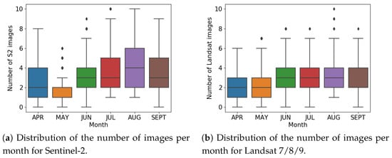
Figure 3.
Distribution of the number of images per month for Sentinel-2 and Landsat 7/8/9 data between 2017 and 2022. Points outside the boxplot whiskers correspond to fields lying on two relative orbits.
2.2.2. Biophysical Parameters
The estimation of Leaf Area Index (LAI) and Leaf Chlorophyll Content () was facilitated using an Artificial Neural Network (ANN) pre-trained on the raw Sentinel-2 bands accessible within the Sentinel Application Platform (SNAP) [29]. These biophysical parameters are of particular interest due to their ability to enhance the signal-to-noise ratio compared to raw bands and/or vegetation indices when predicting maize yield for a new season using Sentinel-2 data [26].
The time series were linearly interpolated and smoothed using the Savitzky–Golay filter, which is commonly used to smooth noisy signals [30,31]. A half-width size of 15 was used for the smooth window, and a third-degree polynomial was used to set the weighting coefficient.
2.2.3. Land Surface Temperature
Land Surface Temperature (LST) was derived by applying the single-channel algorithm [32] to Landsat 8 Band 10 and Landsat 7 Band 6. For consistency, all raw band pixels were resampled to a 50-meter reference grid using nearest neighbor interpolation. Additionally, a binary erosion of radius 1 was applied to eliminate border pixels around the field. In subsequent analyses, pixels identified as cloud and shadow masks, based on thresholding the quality assessment (QA) band, were discarded. The percentage of identified invalid pixels was then calculated relative to the total number of pixels within the field bounding box. Only acquisition dates with more than 50% valid pixels were retained for the analysis.
The time series underwent linear interpolation and smoothing using the Savitzky–Golay filter [30]. Outliers were masked out initially by applying an empirical threshold of 10 °C between day of the year 100 and day of the year 300.
2.3. Agroclimatic Data
In addition to Sentinel-2 optical imagery to monitor seasonal changes and Land Surface Temperature (LST) for drought assessment, our objective was to develop early stress indicators impacting future yield potential. This involved assessing extreme weather conditions like drought, hail, floods, frost, high temperatures, and strong winds, known to have a considerable impact on corn productivity [33].
Previous research has highlighted precipitation and air temperature during the growing season, particularly during the late vegetative and early reproductive stages, as possible influence factors for corn yield deviations [34]. Excessive heat can negatively impact physiological processes, including water stress, root growth, flowering, and lead to premature maturity and senescence [35]. Temperature was found to be more influential than rainfall in estimating corn yield, with rainfall during May and August being relatively less important [36]. Moreover, Johnson [2] showed that precipitations have no correlation with corn yields regardless of the seasonality for midsummer corn yield forecasting at the county level. Given these contradictions and the inclusion of both irrigated and rainfed fields in the study, integration of information related to crop water requirements was avoided.
In order to comprehensively capture temperature dynamics throughout the study period, additional agrometeorological information was incorporated. This included daily means, minimums and maximums, as well as the number of days with temperatures above 30 °C (86 °F) and the accumulated number of Growing Degree Days (GDD). These temperature-related variables were selected because of their proven influence on maize growth and development [25].
ERA5, a high-resolution reanalysis dataset (https://www.sciencedirect.com/topics/engineering/reanalysis, accessed on 10 October 2023) produced by ECMWF (European Centre for Medium-Range Weather Forecasts), was used to obtain historical weather data. However, these data has a time lag of approximately two months and is not available in real-time. To ensure timely forecasts and to place themselves in a operational scenario, we used ERA5T, which is an initial release data available with a time lag of around 5 days.
Table 2 presents a summary of the variables considered to address the early season forecasting of corn yield at the field-level. These variables were derived from daily time series data, which were aggregated into periods, as detailed in Section 3.1.
Table 2.
Variables used in crop yield forecasting during 2017–2022.
3. Methods
In this section, the established early season yield prediction strategy is presented. Yield forecasting is performed for an ongoing season in which harvest data are not yet available, i.e., extrapolating yield to test samples using machine learning methods trained on data from other years.
Section 3.1 briefly introduces the temporal resampling of the time series used in this study, based on thermal rather than calendar time. In Section 3.2.1, the proposal is made to adapt the model inference according to the number of periods available, rather than imputing or deleting missing observations as a baseline. Then, it is suggested to enrich the partially available early season dataset from the full dataset, in terms of time period, available from other years (e.g. historical data). To this end, Section 3.2.2 introduces the workflow to predict an extra period for each field, which will then be used as an observation for the inference phase.
3.1. Temporal Resampling
To resample the time series data based on different temporal criteria, two approaches were adopted. Firstly, for calendar time, the data was divided into fixed 9-day periods starting from the crop fields’ sowing date.
Thermal time offers the advantage of mitigating potential temporal shifts across seasons or locations [37]. Measured in growing-degree days (GDDs), thermal time accumulates mean daily air temperatures at 2 meters above the ground, surpassing a crop-specific threshold. While the accumulation of GDDs over the growing season can vary by location and year, the thermal time required for corn plants to reach specific developmental stages remains relatively constant [38]. This computation can be expressed as follows:
where and denote the minimum and maximum daily temperatures for a given day i, respectively, and represents the base temperature for corn, conventionally set at 10 °C to account for limited growth below this threshold. The upper threshold temperature was typically fixed at 30 °C, assuming a relatively consistent development rate between these two thresholds.
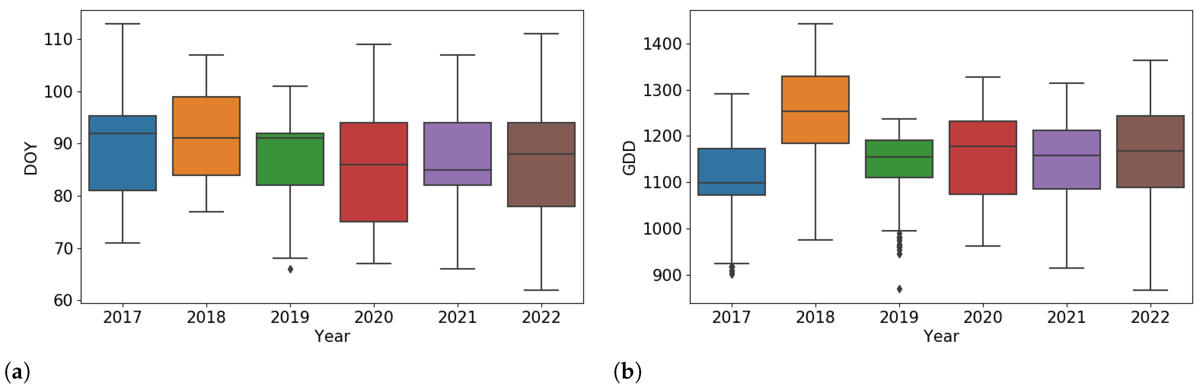
The time series data was aggregated at intervals corresponding to the accumulation of 120 GDDs, as suggested in [26]. Figure 4 displays the distribution of elapsed days and accumulated Growing Degree Days (GDDs) since planting. Generally, the variability in time units between sowing and the cut-off date (August 15th) was less pronounced than that of GDDs.
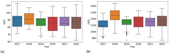
Figure 4.
Distribution of the number of days (calendar or thermal) (a) and accumulated Growing Degree Days (GDDs) between the planting date and the 15th of August across different years (b). These boxplots illustrate the variability in the dataset distribution throughout the growing season, providing insights into the temporal patterns of crop development.
The final period was retained if it covered at least 80% of the chosen time unit before mid-August. This translated to a minimum duration of 7 days and an accumulation of 95 Growing Degree Days (GDDs) for both calendar and thermal time analyses, respectively. This completeness rule applied solely to fields in the current season for which yield forecasting was conducted, as the entire season’s data were available from the training years. Figure 5a,b illustrate the percentage of fields in the dataset that reached the final periods for both calendar and thermal time analyses, corresponding to periods 7 through 10.
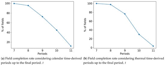
Figure 5.
Percentage of fields reaching a certain period after resampling of time series (calendar (a) or thermal time (b)) at 15 August.
3.2. Yield Estimation Methods
3.2.1. Adapting to Field Progress with Multiple Random Forest Models
In the previous subsection, the issue of missing periods for early season forecasting was addressed, stemming from later sowing dates (calendar time) or lower temperature regimes (thermal time). A straightforward solution would involve deleting the periods for which values are missing. However, this approach would discard part of the available information. To maximize the use of the available data, we propose a strategy to accommodate the number of periods for each field.
Regarding the choice of the machine learning algorithm, Random Forest (RF) [39] has demonstrated considerable successful in predicting corn yield using Sentinel-2 data [13] and Landsat data [5,24]. The scikit-learn package [40] was employed for implementation, with all models empirically parameterized with 500 trees and a maximum depth of 7, while all other parameters were set to their default values. Figure 6 depicts our early season inference strategy, wherein Random Forest (RF) machine learning methods trained on data from previous years are tested. We evaluated early season yield forecasting for each year independently, training the model on data from the years excluding the one being predicted, thereby treating each season as an independent entity.
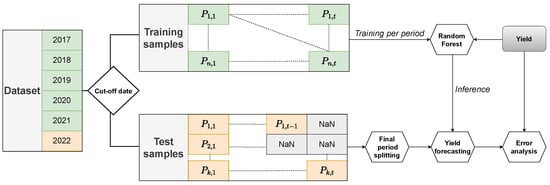
Figure 6.
Training and inference procedure during a new season (e.g., 2022). A cut-off date is applied to the test samples, resulting in missing periods P as each field progresses. We retain all periods in the training samples that correspond to the most advanced period observed in the test samples. Individual models are then calibrated for each of the last periods observed in the test samples (e.g., ). Training years are shown in green, while the test year is shown in orange.
3.2.2. Forecasting Seasonal Trajectories Using Comprehensive Historical Data
The forecasting of was proposed as it has been shown to be the best yield predictor derived from Sentinel-2 data [26]. All available information prior to the cut-off date, derived from Sentinel-2 (S2), crop stress indices (CS) from agroclimatic data, and Land Surface Temperature (LST) from Landsat, was considered. This multivariate approach was preferred over a univariate method that would neglect potential stress factors that could later influence the temporal trajectories of , such as earlier and more abrupt senescence. In previous work, statistical models based on climatic factors such as precipitation and temperature have been applied to predict the seasonal trajectories of the NDVI vegetation index [41,42,43].
A Deep Neural Network (DNN), integrating a Long Short-Term Memory (LSTM) layer [44] to model the inputs with a time dimension was proposed. LSTM layers are designed to model information from long time periods and effectively mitigate the issue of vanishing gradients. Additionally, a data augmentation strategy was considered, in which time series profiles of the 15% and 85% quantiles derived from Sentinel-2 data aggregated to the field level were included, together with the median values previously obtained. This approach aims to leverage additional factors and predict a potential accelerated decrease in the trajectory after the reproductive stage, capturing dynamic changes induced by potential stressors that the model can get profit on.
The output of the DNN was specifically designed to predict the M periods ahead that can be forecasted along the trajectory at period t. These predicted periods are denoted by . Our objective was to capture the contextual information of the seasonal trajectory more effectively through their temporal dependencies by considering a wider forecast horizon than the available one. This would allow the model to gain a deeper understanding of the underlying dynamics, resulting in more accurate and reliable forecasts for the initially desired forecast horizon. The forecast value for , denoted as , can be expressed as follows:
In the DNN architecture (Figure 7), "static" data are incorporated into the training dataset, referring to data with fixed values throughout the season. This includes important information such as the relative maturity of the variety, which can impact the observed phenology during the season, characterized indirectly by the time series of . To incorporate these data, a two-branch approach was employed. One branch consists of Dense (or Fully Connected) layers dedicated to processing the static inputs, while the other branch utilizes an LSTM layer to handle the time-dependent inputs. Merging or combining the internal representations of the two data types in subsequent dense layers via concatenation allows static and temporal information to be integrated, enabling the model to leverage the full set of available information to forecast the seasonal trajectory.
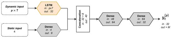
Figure 7.
DNN architecture with LSTM and dense layers. Concatenation of dynamic and static paths. Node dimensions indicated. Each dense hidden layer is followed by batch normalization and ReLU activation function with a dropout rate of 0.5. DNN was trained over 100 epochs with a batch size of 32, learning rate of 10e−4 using the Adam optimizer. Implemented through the Tensorflow library [45].
The Huber loss function was chosen [46]. This loss is characterized by a threshold (the threshold) to allow a transition between mean absolute error (MAE) and mean squared error (MSE), with the aim to handle both outliers and small errors in the prediction model. If denotes the corresponding real value, the loss can be defined as follows:
4. Results and Discussion
In this section, the results of our different preprocessing techniques and early season yield estimation strategies, constituting our contribution as outlined in Section 3.2, are presented. Two evaluation metrics, R-squared () and MAPE (Mean Absolute Percentage Error), were utilized to assess the performance of the methods.
In Section 4.1, an evaluation of the two temporal resampling techniques for time series observations (calendar and thermal time) is presented using the method. Then, in Section 4.2, the impact of different data sources on the evaluation metrics of the early season model was examined. Then, in Section 4.3, the results of the yield prediction model are presented, where the first step involves predicting one period of ahead for the test samples, which are then used in model inference during the season. In Section 4.4, detailed results are provided for predicting the yield for each season independently in mid-August with the most effective strategy we have designed. Finally, in Section 4.5.2, we draw possible future perspectives, taking into account the conclusions drawn from the analyses described earlier.
4.1. Comparison between Calendar and Thermal Time Temporal Resampling
For accurate results with the early season strategy outlined in Section 3.2.1, the model was employed. This model trains a separate RF model for each period and utilizes the last observed period as a rule for inference in the test samples. Resampling the time series over thermal time has led to a reduction in the mean absolute percentage error from 17.02% to 16.25% and an increase in the proportion of yield variability explained by the model () from 0.25 to 0.30 (Table 3).
Table 3.
MAPE and evaluation metrics around the 15 August. The values reported are mean ± standard deviation.
4.2. Contribution of Different Data Sources to Early Season Forecasting
In Table 2, various data sources were compared: biophysical variables from Sentinel-2 (S2), a combination of Sentinel-2 data with Land Surface Temperature (LST) (S2 + LST), and the integration of these sources with crop stress indices (CS) from agroclimatic data (S2 + LST + CS). Additionally, end-of-season metrics () were presented, utilizing a total of 14 periods for both training and testing. This allowed for the assessment of the early season forecasting strategy against predictions made with comprehensive data. The aim was to determine if the identified variables were beneficial solely for early season crop yield forecasting or had broader applicability for strategies informed at the end of the season.
Table 4 and Table 5 provide the average and standard deviations of the MAPE and scores, respectively. Considering Land Surface Temperature (LST) as a data source resulted in a reduction of the MAPE error for the model from 16.54% to 16.39% and a significant increase in the proportion of variance explained, from 0.26 to 0.29. Subsequent addition of agroclimatic crop stress indices (CS) further improved the results, leading to a MAPE of 16.25%. These findings confirm the effectiveness of LST and CS in detecting early stress during the growing season. However, there was no observed improvement in the performance of the model with the inclusion of these factors, suggesting that the optical data alone were sufficient for end-of-season forecasting.
Table 4.
MAPE evaluation metric per data source. The values reported are mean ± standard deviation.
Table 5.
evaluation metric per data source. The values reported are mean ± standard deviation.
4.3. Leverage Out-of-Year Data to Refine Early Season Yield Forecasts
Chlorophyll-a and b (C) values were forecasted one period ahead for each test sample using the DNN method. These forecasts were then integrated into corn yield forecasting with , aiming to expand the early season time series. During inference, RF models were determined based on the last predicted period. Evaluation measures for this approach, labeled DNN, are presented in Table 6.
Table 6.
and MAPE evaluation metrics when using whose period breakdown depends on the last period observed at the cut-off date plus a period predicted by DNN. The values reported are mean ± standard deviation.
Our strategy, that consists in the use of the DNN to impute the next period of a test sample from a given year, showed the most promising performance among all the evaluated methods. It achieved an MAPE of 16.09%. These results confirm the potential of using out-of-year (e.g. historical data) after the cut-off date to extend data acquired during the ongoing season for the early season yield forecasting task. Figure 8 presents a bar chart of the MAPE and evaluation metrics by year. It is evident that a systematic improvement, across all seasons, exists thus, resulting in increased values or decreased MAPE, except for 2019 where we observed a slight degradation in results. This could be attributed, in part, to the limited availability of Landsat images used for estimating LST during that season.
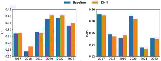
Figure 8.
Model performance evaluation for early season yield forecasting in an independent test year, illustrated by R-squared (left) and MAPE (right). The baseline method (blue) is compared with , incorporating an additional period predicted by DNN, for period breakdown (orange).
4.4. Fine Evaluation of the Best Early Season Strategy
4.4.1. Impact of Available Images on Accuracy
The correlation between the number of available images and the mean absolute error (in percentage) for in-season yield forecasts, generated at the cut-off date of 15 August using evaluation data from years not included in model training, was investigated. In Figure 9, the number of S2 images between May and July was categorized into four bins, and the mean error was calculated, with the standard deviation illustrating the variability across years. A clear correlation between the number of available images and model performance was observed. Specifically, a significant improvement was noted when the number of images exceeded 12 during this period, indicating an average of at least one image per week.

Figure 9.
Mean Absolute Percentage Error (MAPE) computed across different total ranges of Sentinel-2 images available from May to August. The standard deviation, calculated across multiple years, is represented by the bars.
4.4.2. Visual Inspection
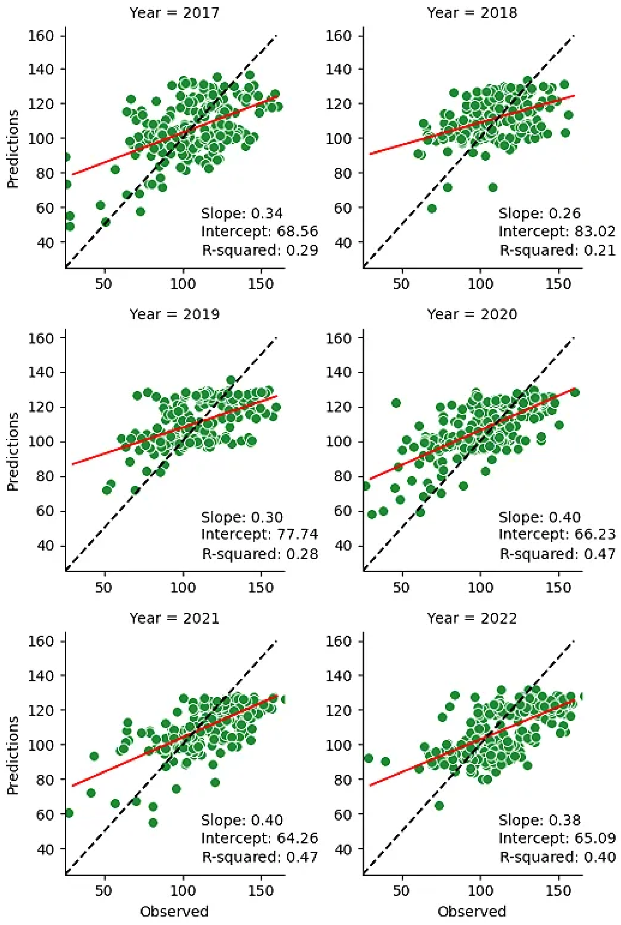
To quantitatively and qualitatively assess the yield forecasts, the extent to which the predicted and observed yields aligned with the 45° line passing through the origin (representing a perfect correspondence between predicted and observed) was examined. In Figure 10, scatter plots of observed corn yields against predicted yields are presented. The alignment of predicted and observed yields on the 45° line through the origin was satisfactory for 2020, 2021, and 2022. However, for 2017 and 2018, the predicted values were positively correlated but struggled to explain much of the variance around the observed mean values of corn yields. These results suggest the ability to predict a trend in maize yields averaged over at field scale.
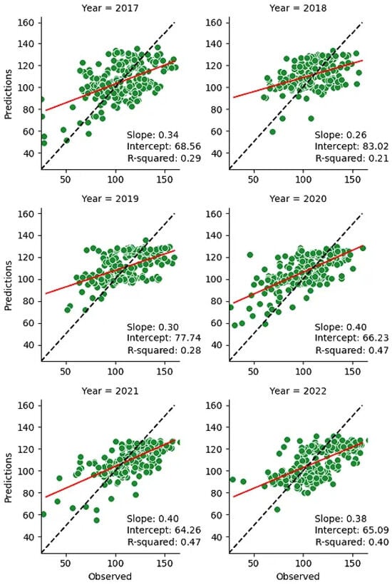
Figure 10.
These scatter plots depict the correlation between observed (x-axis) and predicted (y-axis) yield values obtained using DNN (Deep Neural Network) models. The black dashed line represents the ideal 45° line of perfect prediction, while the red line indicates the linear regression fit of the scatter plot, accompanied by the fitting metric reported.
4.5. Limitations and Perspectives
4.5.1. Limitations
Satellite-derived data covers only a portion of the spectrum of actual crop yield variation. Optical data primarily reflects the photosynthetically active biomass within fields but may not fully capture grain yield, which depends on multiple factors [47]. Despite this limitation, our approach to early season yield prediction using freely available remote sensing data offers valuable advantages for monitoring crop growth and development throughout the season at the field scale. Emphasizing the use of imagery acquired up to the first half of August, the scalable nature of our framework enables extensive monitoring at field scale, thus potentially providing benefits to farmers and other stakeholders involved in farm management.
Another inherent limitation of our approach concerns data availability. Although our method assumes the presence of at least one image during the first half of August, practical implementation can be affected by variations in image availability, which can affect forecast accuracy. Data limitation also applies to the use of meteorological data from ERA5T, which only provides weather information up to five days before the current date. This time constraint may lead to delays in providing larger-scale forecasts, as our approach requires a lead time of around five days.
4.5.2. Future Work
There are several ways to further advance the forecasting of maize yield. One approach is to incorporate soil surface temperature (LST) into the Soil Surface Energy Balance Algorithm (SEBAL) [48] for more effective early season yield prediction and drought monitoring. LST data provides insights into energy flows and water stress in agricultural systems, enhancing estimates of evapotranspiration and crop water requirements. Integrating indicators of cumulative drought [5] or crop water requirements into the forecasting models would compensate for the limitations of optical satellite data, which primarily measure canopy surface potential and may underestimate the negative impacts of drought on yield [18]. This approach would be the most appropriate if we had precise information on irrigation dates and doses throughout the season. Additionally, utilizing finer-scale weather data, such as PRISM (https://prism.oregonstate.edu/, accessed on 10 October 2023), tailored to specific regions in the United States, could improve the accuracy and localization of yield predictions.
Secondly, from a methodological point of view, investigations of alternative machine learning methods can bring some additional values. In [26], the authors concluded that no single machine learning regression model emerged as a clear winner in predicting yield values for a new season, and performance can vary depending on the year. The authors suggested using a Stacked Averaging Ensemble (SAE) that combines multiple models could potentially outperform individual models, necessitating the optimization of hyperparameters using a leave-one-year-out validation strategy. This is particularly important for sensitive models like Support Vector Machines (SVM) or Extreme Gradient Boosting (XGBoost).
5. Conclusions
This study analyzed and compared the performance of data-driven methods for early season corn yield forecasting (mid-August) from ground-based data in the U.S. using Sentinel-2, Landsat 7/8/9, agroclimatic and in-situ data. The capacity of estimating yield based on out-of-year corn yield seeds production dataset was shown to be influenced by various aspects, namely: (1) the way in which temporal dynamic is considered (thermal or calendar); (2) the way we take into account the progress of the field based on thermal time by inferring a different model regarding the last period available; (3) how we could exploit the full seasonal trajectory information derived from Sentinel-2 data available in the training years to better infer the current season by forecasting the next period for the test samples. By resampling the time series over thermal time, building a per-period model based on expected field advancement, and predicting the short-term seasonal trend of using a DNN, our early season yield estimation approach explained 31% of the yield variation, with an associated MAPE of 16.1%. This early season result (estimated around mid-August) remains more than comparable to the MAPE achieved at the end of the season (Mid-October) that is estimated to 15.2%. This result suggests that valuable yield crop estimation (comparable to end of season) can be obtained early in the season, possibly providing farmers with an estimate of their production two months before the harvest time.
Author Contributions
J.D.: Conceptualization, Methodology, Software, Validation, Formal analysis, Investigation, Data Curation, Writing—Original Draft, Writing—Review and Editing, Visualization. D.I.: Conceptualization, Methodology, Writing—Review and Editing, Supervision, Project Administration, Resources, Funding Acquisition. A.B.: Validation, Supervision, Project Administration, Resources, Funding Acquisition. All authors have read and agreed to the published version of the manuscript.
Funding
This research was funded by the French National Association of Research and Technology through the Convention Industrielle de Formation par la REcherche (CIFRE refered as 2019/1993) Ph.D. Grant.
Data Availability Statement
The original contributions presented in the study are included in the article, further inquiries can be directed to the corresponding author.
Acknowledgments
The authors would like to thank the European Space Agency (ESA), France for sponsoring the SentinelHub account as part of the Network of Resources (NoR) program, and Syngenta Production and Supply for making its agronomic data available.
Conflicts of Interest
The authors J.D. and A.B were employed by the company Syngenta. The remaining author D.I. declares that the research was conducted in the absence of any commercial or financial relationships that could be construed as a potential conflict of interest.
Abbreviations
The following abbreviations are used in this manuscript:
| ANN | Artficial Neural Network |
| Leaf Chlorophyll Content (g/cm−2) | |
| DNN | Deep Neural Network |
| ERA5 | ECMWF ReAnalysis 5 |
| GDD | Growing Degree Days |
| LST | Land Surface Temperature |
| LSTM | Long Short Term Memory |
| MAPE | Mean Absolute Percentage Error |
| NDVI | Normalized Difference Vegetation Index |
| RF | Random Forest |
| S2 | Sentinel-2 |
| SNAP | Sentinel Application Platform |
References
- Zhao, Y.; Potgieter, A.B.; Zhang, M.; Wu, B.; Hammer, G.L. Predicting wheat yield at the field scale by combining high-resolution Sentinel-2 satellite imagery and crop modelling. Remote Sens. 2020, 12, 1024. [Google Scholar] [CrossRef]
- Johnson, D.M. An assessment of pre-and within-season remotely sensed variables for forecasting corn and soybean yields in the United States. Remote Sens. Environ. 2014, 141, 116–128. [Google Scholar] [CrossRef]
- Beres, B.L.; Hatfield, J.L.; Kirkegaard, J.A.; Eigenbrode, S.D.; Pan, W.L.; Lollato, R.P.; Hunt, J.R.; Strydhorst, S.; Porker, K.; Lyon, D.; et al. Toward a Better Understanding of Genotype × Environment × Management Interactions—A Global Wheat Initiative Agronomic Research Strategy. Front. Plant Sci. 2020, 11, 89–93. [Google Scholar] [CrossRef] [PubMed]
- Tewes, A.; Hoffmann, H.; Krauss, G.; Schäfer, F.; Kerkhoff, C.; Gaiser, T. New approaches for the assimilation of LAI measurements into a crop model ensemble to improve wheat biomass estimations. Agronomy 2020, 10, 446. [Google Scholar] [CrossRef]
- Shuai, G.; Basso, B. Subfield maize yield prediction improves when in-season crop water deficit is included in remote sensing imagery-based models. Remote Sens. Environ. 2022, 272, 112938. [Google Scholar] [CrossRef]
- Carletto, C.; Jolliffe, D.; Banerjee, R. From tragedy to renaissance: Improving agricultural data for better policies. J. Dev. Stud. 2015, 51, 133–148. [Google Scholar] [CrossRef]
- Van Klompenburg, T.; Kassahun, A.; Catal, C. Crop yield prediction using machine learning: A systematic literature review. Comput. Electron. Agric. 2020, 177, 105709. [Google Scholar] [CrossRef]
- FAO. Handbook for Defining and Setting up a Food Security Information and Early Warning System (FSIEWS); FAO: Rome, Italy, 2000. [Google Scholar]
- Chipanshi, A.; Zhang, Y.; Kouadio, L.; Newlands, N.; Davidson, A.; Hill, H.; Warren, R.; Qian, B.; Daneshfar, B.; Bedard, F.; et al. Evaluation of the Integrated Canadian Crop Yield Forecaster (ICCYF) model for in-season prediction of crop yield across the Canadian agricultural landscape. Agric. For. Meteorol. 2015, 206, 137–150. [Google Scholar] [CrossRef]
- Johnson, D.M.; Mueller, R. Pre-and within-season crop type classification trained with archival land cover information. Remote Sens. Environ. 2021, 264, 112576. [Google Scholar] [CrossRef]
- Kanke, Y.; Tubana, B.; Dalen, M.; Harrell, D. Evaluation of red and red-edge reflectance-based vegetation indices for rice biomass and grain yield prediction models in paddy fields. Precis. Agric. 2016, 17, 507–530. [Google Scholar] [CrossRef]
- Gascon, F.; Bouzinac, C.; Thépaut, O.; Jung, M.; Francesconi, B.; Louis, J.; Lonjou, V.; Lafrance, B.; Massera, S.; Gaudel-Vacaresse, A.; et al. Copernicus Sentinel-2A calibration and products validation status. Remote Sens. 2017, 9, 584. [Google Scholar] [CrossRef]
- Kayad, A.; Sozzi, M.; Gatto, S.; Marinello, F.; Pirotti, F. Monitoring Within-Field Variability of Corn Yield using Sentinel-2 and Machine Learning Techniques. Remote Sens. 2019, 11, 2873. [Google Scholar] [CrossRef]
- Li, F.; Miao, Y.; Chen, X.; Sun, Z.; Stueve, K.; Yuan, F. In-Season Prediction of Corn Grain Yield through PlanetScope and Sentinel-2 Images. Agronomy 2022, 12, 3176. [Google Scholar] [CrossRef]
- Kang, Y.; Özdoğan, M. Field-level crop yield mapping with Landsat using a hierarchical data assimilation approach. Remote Sens. Environ. 2019, 228, 144–163. [Google Scholar] [CrossRef]
- Wang, Q.; Blackburn, G.A.; Onojeghuo, A.O.; Dash, J.; Zhou, L.; Zhang, Y.; Atkinson, P.M. Fusion of Landsat 8 OLI and Sentinel-2 MSI data. IEEE Trans. Geosci. Remote Sens. 2017, 55, 3885–3899. [Google Scholar] [CrossRef]
- Khanal, S.; Fulton, J.; Shearer, S. An overview of current and potential applications of thermal remote sensing in precision agriculture. Comput. Electron. Agric. 2017, 139, 22–32. [Google Scholar] [CrossRef]
- Thelen, K. Assessing Drought Stress Effects on Corn Yield. Field Crop Advisory Team Alert Newsletter. Michigan State Univ. 2007. Available online: http://msue.anr.msu.edu/news/assessing (accessed on 10 October 2023).
- Pede, T.; Mountrakis, G.; Shaw, S.B. Improving corn yield prediction across the US Corn Belt by replacing air temperature with daily MODIS land surface temperature. Agric. For. Meteorol. 2019, 276, 107615. [Google Scholar] [CrossRef]
- Palosuo, T.; Kersebaum, K.C.; Angulo, C.; Hlavinka, P.; Moriondo, M.; Olesen, J.E.; Patil, R.H.; Ruget, F.; Rumbaur, C.; Takáč, J.; et al. Simulation of winter wheat yield and its variability in different climates of Europe: A comparison of eight crop growth models. Eur. J. Agron. 2011, 35, 103–114. [Google Scholar] [CrossRef]
- Behmann, J.; Mahlein, A.K.; Rumpf, T.; Römer, C.; Plümer, L. A review of advanced machine learning methods for the detection of biotic stress in precision crop protection. Precis. Agric. 2015, 16, 239–260. [Google Scholar] [CrossRef]
- Schwalbert, R.; Amado, T.; Nieto, L.; Corassa, G.; Rice, C.; Peralta, N.; Schauberger, B.; Gornott, C.; Ciampitti, I. Mid-season county-level corn yield forecast for US Corn Belt integrating satellite imagery and weather variables. Crop Sci. 2020, 60, 739–750. [Google Scholar] [CrossRef]
- Ma, Y.; Zhang, Z.; Yang, H.L.; Yang, Z. An adaptive adversarial domain adaptation approach for corn yield prediction. Comput. Electron. Agric. 2021, 187, 106314. [Google Scholar] [CrossRef]
- Deines, J.M.; Patel, R.; Liang, S.Z.; Dado, W.; Lobell, D.B. A million kernels of truth: Insights into scalable satellite maize yield mapping and yield gap analysis from an extensive ground dataset in the US Corn Belt. Remote Sens. Environ. 2021, 253, 112174. [Google Scholar] [CrossRef]
- Duveiller, G.; Frederic, B.; Defourny, P. Using Thermal Time and Pixel Purity for Enhancing Biophysical Variable Time Series: An Interproduct Comparison. IEEE Trans. Geosci. Remote Sens. 2013, 51, 2119–2127. [Google Scholar] [CrossRef]
- Desloires, J.; Ienco, D.; Botrel, A. Out-of-year corn yield prediction at field-scale using Sentinel-2 satellite imagery and machine learning methods. Comput. Electron. Agric. 2023, 209, 107807. [Google Scholar] [CrossRef]
- Van Donk, S.J.; Petersen, J.L.; Davison, D.R. Effect of amount and timing of subsurface drip irrigation on corn yield. Irrig. Sci. 2013, 31, 599–609. [Google Scholar] [CrossRef]
- Main-Knorn, M.; Pflug, B.; Louis, J.; Debaecker, V.; Müller-Wilm, U.; Gascon, F. Sen2Cor for Sentinel-2. In Proceedings of the Image and Signal Processing for Remote Sensing XXIII, Warsaw, Poland, 11–13 September 2017; 10427, p. 3. [Google Scholar]
- Weiss, M.; Baret, F. S2ToolBox Level 2 Products: LAI, FAPAR, FCOVER; Institut National de la Recherche Agronomique (INRA): Avignon, France, 2016. [Google Scholar]
- Savitzky, A.; Golay, M.J.E. Smoothing and Differentiation of Data by Simplified Least Squares Procedures. Anal. Chem. 1964, 36, 1627–1639. [Google Scholar] [CrossRef]
- Shao, Y.; Lunetta, R.S.; Wheeler, B.; Iiames, J.S.; Campbell, J.B. An evaluation of time-series smoothing algorithms for land-cover classifications using MODIS-NDVI multi-temporal data. Remote Sens. Environ. 2016, 174, 258–265. [Google Scholar] [CrossRef]
- Jiménez-Muñoz, J.C.; Sobrino, J.A. A single-channel algorithm for land-surface temperature retrieval from ASTER data. IEEE Geosci. Remote Sens. Lett. 2009, 7, 176–179. [Google Scholar] [CrossRef]
- Ortez, O.A.; McMechan, A.J.; Hoegemeyer, T.; Ciampitti, I.A.; Nielsen, R.L.; Thomison, P.R.; Abendroth, L.J.; Elmore, R.W. Conditions potentially affecting corn ear formation, yield, and abnormal ears: A review. Crop Forage Turfgrass Manag. 2022, 8, e20173. [Google Scholar] [CrossRef]
- Teasdale, J.R.; Cavigelli, M.A. Meteorological fluctuations define long-term crop yield patterns in conventional and organic production systems. Sci. Rep. 2017, 7, 688. [Google Scholar] [CrossRef]
- Schauberger, B.; Archontoulis, S.; Arneth, A.; Balkovič, J.; Ciais, P.; Deryng, D.; Elliott, J.; Folberth, C.; Khabarov, N.; Müller, C.; et al. Consistent negative response of US crops to high temperatures in observations and crop models. Nat. Commun. 2017, 8, 13931. [Google Scholar] [CrossRef] [PubMed]
- Joshi, V.R.; Kazula, M.J.; Coulter, J.A.; Naeve, S.L.; Garcia y Garcia, A. In-season weather data provide reliable yield estimates of maize and soybean in the US central Corn Belt. Int. J. Biometeorol. 2021, 65, 489–502. [Google Scholar] [CrossRef] [PubMed]
- Atwell, B.; Kriedemann, P.; Turnbull, C. Plants in Action: Adaption in Nature, Performance in Cultivation, 1st ed.; Macmillan Education: Melbourne, Australia, 1999. [Google Scholar]
- Nleya, T.; Chungu, C.; Kleinjan, J. Corn Growth and Development; North Dakota State University: Bismarck, ND, USA, 2019; pp. 5–8. [Google Scholar]
- Breiman, L. Random Forests. Mach. Learn. 2001, 45, 5–32. [Google Scholar] [CrossRef]
- Pedregosa, F.; Varoquaux, G.; Gramfort, A.; Michel, V.; Thirion, B.; Grisel, O.; Blondel, M.; Prettenhofer, P.; Weiss, R.; Dubourg, V.; et al. Scikit-learn: Machine learning in Python. J. Mach. Learn. Res. 2011, 12, 2825–2830. [Google Scholar]
- Propastin, P.A.; Kappas, M. Reducing uncertainty in modeling the NDVI-precipitation relationship: A comparative study using global and local regression techniques. GISci. Remote Sens. 2008, 45, 47–67. [Google Scholar] [CrossRef]
- Fernández-Manso, A.; Quintano, C.; Fernández-Manso, O. Forecast of NDVI in coniferous areas using temporal ARIMA analysis and climatic data at a regional scale. Int. J. Remote Sens. 2011, 32, 1595–1617. [Google Scholar] [CrossRef]
- Gao, P.; Du, W.; Lei, Q.; Li, J.; Zhang, S.; Li, N. NDVI Forecasting Model Based on the Combination of Time Series Decomposition and CNN–LSTM. Water Resour. Manag. 2023, 37, 1481–1497. [Google Scholar] [CrossRef]
- Hochreiter, S.; Schmidhuber, J. Long short-term memory. Neural Comput. 1997, 9, 1735–1780. [Google Scholar] [CrossRef] [PubMed]
- Abadi, M.; Barham, P.; Chen, J.; Chen, Z.; Davis, A.; Dean, J.; Devin, M.; Ghemawat, S.; Irving, G.; Isard, M.; et al. Tensorflow: A system for large-scale machine learning. In Proceedings of the 12th {USENIX} Symposium on Operating Systems Design and Implementation ({OSDI} 16), Savannah, GA, USA, 2–4 November 2016; pp. 265–283. [Google Scholar]
- Huber, P.J. Robust Estimation of a Location Parameter. Ann. Stat. 1964, 53, 73–101. [Google Scholar] [CrossRef]
- Rudorff, B.; Batista, G. Spectral response of wheat and its relationship to agronomic variables in the tropical region. Remote Sens. Environ. 1990, 31, 53–63. [Google Scholar] [CrossRef]
- Laipelt, L.; Kayser, R.H.B.; Fleischmann, A.S.; Ruhoff, A.; Bastiaanssen, W.; Erickson, T.A.; Melton, F. Long-term monitoring of evapotranspiration using the SEBAL algorithm and Google Earth Engine cloud computing. ISPRS J. Photogramm. Remote Sens. 2021, 178, 81–96. [Google Scholar] [CrossRef]

Disclaimer/Publisher’s Note: The statements, opinions and data contained in all publications are solely those of the individual author(s) and contributor(s) and not of MDPI and/or the editor(s). MDPI and/or the editor(s) disclaim responsibility for any injury to people or property resulting from any ideas, methods, instructions or products referred to in the content. |
© 2024 by the authors. Licensee MDPI, Basel, Switzerland. This article is an open access article distributed under the terms and conditions of the Creative Commons Attribution (CC BY) license (https://creativecommons.org/licenses/by/4.0/).