Article

Wheat Yield Robust Prediction in the Huang-Huai-Hai Plain by Coupling Multi-Source Data with Ensemble Model under Different Irrigation and Extreme Weather Events

National Engineering and Technology Center for Information Agriculture, Key Laboratory for Crop System Analysis and Decision Making, Jiangsu Collaborative Innovation Center for Modern Crop Production, Nanjing Agricultural University, 1 Weigang Road, Nanjing 210095, China
*
Author to whom correspondence should be addressed.
These authors contributed equally to this work.
Remote Sens. 2024, 16(7), 1259; https://doi.org/10.3390/rs16071259
Submission received: 4 March 2024 / Revised: 25 March 2024 / Accepted: 29 March 2024 / Published: 2 April 2024
(This article belongs to the Special Issue Within-Season Agricultural Monitoring from Remotely Sensed Data)

Abstract

:
The timely and robust prediction of wheat yield is very significant for grain trade and food security. In this study, the yield prediction model was developed by coupling an ensemble model with multi-source data, including vegetation indices (VIs) and meteorological data. The results showed that green chlorophyll vegetation index (GCVI) is the optimal remote sensing (RS) variable for predicting wheat yield compared with other VIs. The accuracy of the adaptive boosting- long short-term memory (AdaBoost-LSTM) ensemble model was higher than the LSTM model. AdaBoost-LSTM coupled with optimal input data had the best performance. The AdaBoost-LSTM model had strong robustness for predicting wheat yield under different irrigation and extreme weather events in general. Additionally, the accuracy of AdaBoost-LSTM for rainfed counties was higher than that for irrigation counties in most years except extreme years. The yield prediction model developed with the characteristic variables of the window from February to April had higher accuracy and smaller data requirements, which was the best prediction window. Therefore, wheat yield can be accurately predicted by the AdaBoost-LSTM model one to two months of lead time before maturity in the HHHP. Overall, the AdaBoost-LSTM model can achieve accurate and robust yield prediction in large-scale regions.

1. Introduction

Huang-Huai-Hai Plain (HHHP) is an important grain production base in China, with wheat production accounting for over 35% of the country’s total output [1]. Studies on growth monitoring and yield prediction of wheat are beneficial to the accurate grasp of grain production status and the set of government agricultural policies [2,3]. Remote sensing (RS) data can cover a large area and reflect sufficient surface information, with high timeliness and low cost, which provides a new technical method for the fast and precise acquisition of crop growth information [4,5,6].
A traditional yield estimation method combined with RS data directly developed statistical models to predict yield based on the relationship between RS variables (e.g., vegetation indices, VIs) and crop yield [7,8]. However, crop yield formation exhibited nonlinear responses to extreme environment conditions, which may result in a poor performance of previous linear regression models [9,10]. Machine learning (ML) was an advanced method for crop yield estimation and widely used in agriculture-related domains [11,12]. Compared with linear analysis, ML algorithms can capture nonlinear relationships between crops and their external environmental variables. Feng et al. [13] found that the prediction model coupling with an ML algorithm could perform better in wheat yield prediction than that coupling with the multiple linear regression (MLR) algorithm. In recent years, there have been an increasing number of studies on crop yield prediction using ML algorithms in a large-scale region. Cai et al. [14] showed that the prediction model for wheat yield based on the combination of enhanced vegetation index (EVI) and climate variables performed well in southeastern and southwestern Australia. Han et al. [15] developed a county-level wheat yield prediction model based on ML and multi-source data in China and obtained good results. Deep learning (DL) was a more advanced ML algorithm, which was widely applied in crop yield prediction [16,17,18]. As compared with the ML algorithm, DL had better performance in crop yield prediction [19,20]. Zhang et al. [21] found that the yield prediction model using long short-term memory (LSTM) to integrate climate data and vegetation indices outperforms light gradient boosting machine (LightGBM) and least absolute shrinkage and selection operator (LASSO). However, with a limited training dataset, both ML and DL were prone to overfitting [22,23,24,25]. The ensemble model can combine the prediction of several weak learners to make the final prediction, which can obtain better prediction performance [26,27,28,29]. Li et al. [30] integrated multiple ML models with a Bayesian average model to improve the prediction accuracy of maize yield in Northeast China. The adaptive boosting (AdaBoost) algorithm was the more practical boosting algorithm and widely used to improve the performance of weak learners [31,32]. Sun et al. [33] proposed the AdaBoost-LSTM ensemble learning model to predict financial time series, while the AdaBoost-LSTM model outperformed other single prediction models and ensemble models. However, the performance of the AdaBoost-LSTM in crop yield prediction has not been well investigated.
On the other hand, the selection of RS variables had a great influence on the precision of yield prediction. Son et al. [34] found that EVI-based models were slightly more accurate than those from NDVI-based models in the rice yield prediction. Some studies used solar-induced chlorophyll fluorescence (SIF) to predict crop yield [35,36]. Zhou et al. [37] found that SIF had better prediction for yield than traditional VIs (e.g., EVI and NDVI). However, the spatial resolution of existing SIF products was coarse and had much noise [14,38]. This would increase the uncertainty in yield prediction. Recently, near-infrared reflectance (NIRv) has been suggested as the effective substitution of SIF after theoretical derivations and radiative transfer simulations [39], which has been used to estimate GPP, phenology and yield [40,41,42]. Moreover, kernel NDVI (kNDVI) exhibited a stronger correlation than the NDVI and NIRv in some independent products (e.g., GPP and SIF) [43], while there was a marked correlation between the green chlorophyll vegetation index (GCVI) and leaf area index (LAI) [44,45]. The selection of optimal RS variables was very important for the accuracy and robustness of yield prediction.
Given the trade-off between temporal resolution and spatial resolution, complicated phenological information was usually obtained from MODIS images, GLASS LAI data or other low spatial resolution data [46,47]. Nevertheless, plenty of mixed pixels in the classification map would exist due to the status. Accurate acquisition of spatial crop spatial distribution was a prerequisite for growth monitoring and yield prediction [48]. Furthermore, the prediction model generally had different performance under irrigation conditions. Compared with irrigated fields, yield prediction in rainfed fields maybe more accurate [8]. Some researchers will delete samples with irrigation records when conducting yield-related studies [49,50]. The performance of yield prediction models under extreme weather conditions was also noteworthy [14]. Additionally, few studies had systematically analyzed the roles of different input characteristic variable and prediction windows in the yield prediction model.
In this study, the aims were to (1) combine the threshold method with ML algorithm to obtain high-resolution wheat planting area maps at 30 m resolution in the HHHP; (2) use the AdaBoost-LSTM ensemble model to obtain robust prediction of wheat yield in the HHHP under extreme weather events and different irrigation conditions; (3) compare the effects of different VIs and select the optimal VI in yield prediction; and (4) evaluate the optimal prediction window for wheat yield prediction.

2. Data Sources and Methods

2.1. Study Area

There are seven provincial-level administrative regions (Hebei, Shandong, Henan, Anhui, Jiangsu, Beijing and Tianjin) in the HHHP (Figure 1), and 427 counties in the HHHP were selected as the study area. The main cropping system in the study area is the double-cropping system of wheat/maize or wheat/rice, while winter wheat is usually planted in mid-to-late October and harvested in early June. In the study area, the northern region is irrigated agriculture, and the southern region is rainfed agriculture [51]. The region has a warm temperate monsoon climate, while most precipitation appears from July to September.

2.2. Data Sources

The data mainly included satellite data, meteorological data, county-level statistics of wheat planting area and yield and phenology from agro-meteorological stations (Table 1).

2.2.1. Satellite Data

The images from Landsat 5/7/8 and MODIS products used in this study can be obtained on the Google Earth Engine (GEE) platform (Table 1). We can process satellite images by using the immense computing power of Google and improve the efficiency of research in a large-scale region on the GEE platform, which has been widely used in many research fields [52,53]. The temporal resolution and spatial resolution of Landsat images were 16 d and 30 m, respectively. The temporal resolution and spatial resolution of MOD09GA EVI images were 1 d and 500 m, while the temporal resolution and spatial resolution of MOD09A1 images were 8 d and 500 m. According to previous studies, three VIs of satellite images including normalized difference vegetation index (NDVI), normalized difference building index (NDBI) and modified normalized difference water index (MNDWI) were chosen for crop classification. The NDVI is an important parameter reflecting crop growth and is widely used in related fields [54,55,56]. The NDBI and MNDWI were used to distinguish non-crop areas such as buildings and water bodies, respectively [57,58,59,60]. Additionally, the NDVI and other four VIs (including the EVI, kNDVI, GCVI and NIRv) were selected to develop the model for comparison of performance in predicting yield. The relevant calculation formulas were as follows:
NDVI = NIR RED / NIR + RED
NDBI = SWIR 1 NIR / SWIR 1 + NIR
MNDWI = GREEN SWIR 1 / GREEN + SWIR 1
GCVI = NIR GREEN 1
EVI = 2.5 × NIR RED / NIR + 6 × RED 7.5 × BLUE + 1
NIRv = NDVI 0.08 × NIR
kNDVI = tanh NDVI 2
where BLUE, GREEN, RED, NIR and SWIR1 represented blue band, green band, red band, near infrared band and short-wave infrared reflectance band, respectively.

2.2.2. Meteorological Data

The precipitation (Pr), short-wave radiation (Srad), maximum temperature (Tmax), evapotranspiration (ET), minimum temperature (Tmin) and vapor pressure deficit (VPD) data used in this study were obtained from TerraClimate dataset on GEE platform. The TerraClimate dataset was a monthly, ~4 km spatial resolution climate dataset generated by combining the mean climate variables at high spatial resolution from the WorldClim dataset with temporal data at coarse resolution from other data sources. Compared with other climate datasets at coarse spatial resolution, the overall mean absolute error of the dataset was significantly reduced, and the ability to capture spatial features was improved [61].
In addition, given the impact of soil topsoil layer on crop growth [62,63,64], soil moisture (SM) was used as input variables for the wheat yield prediction. SM used in the study was derived from the TerraClimate dataset generated by using a one-dimensional soil water balance model. Therefore, SM was divided into meteorological data for discussion.

2.2.3. Crop Data

Crop data mainly included county-level statistics and field data at experimental stations. County-level statistics mainly referred to the planting area and yield data for wheat, which can be obtained from the China Agricultural Statistical Yearbook. County-level wheat planting data were mainly used to estimate the precision of the wheat planting area extracted in this study, while yield data was used to train and test the yield prediction model. The field data at experimental stations mainly included the phenological information of wheat, which was obtained from China’s Meteorological Administration.

2.3. Methods

A flow chart of this study is shown in Figure 2 and includes two steps: the extraction of the wheat planting area and the development of the wheat yield prediction model.

2.3.1. Extraction of Planting Area

Extraction of the wheat planting area was divided into two steps. Firstly, green up-date (GD) and heading date (HD) of wheat were determined based on MOD09GA images using the dynamic threshold method [65,66] and maximum method [67,68], respectively. The maximum and minimum values of GD and HD were determined according to the phenological characteristics of wheat in the study area, while pixels higher than the maximum value or lower than the minimum value were eliminated. Then the preliminary extraction of the wheat planting area was achieved.
Secondly, cloud-free images from Landsat were unified as monthly intervals (from October to the following May), and MOD09A1 images were processed using bilinear resampling to fill gaps of monthly images due to the limitation of satellite images from Landsat. Then the time series of satellite images during the wheat growth period was reconstructed using the Savitzky–Golay (S–G) filter. Finally, the preliminary extraction results were used to filter out sample points selected according to the phenological information and location information of agro-meteorological stations. Relevant studies showed that five years is the minimum time interval to provide sufficient images for time aggregation [69]. Therefore, wheat planting area maps for 2000, 2005, 2010, 2015 and 2020 were generated by combining the time series images, filtered sample points and random forest (RF) algorithm [70,71]. The statistical data of the wheat planting area at the county level was used to estimate the precision.

2.3.2. Development of Wheat Yield Prediction Model

Firstly, all input data with coarse spatial resolution (e.g., meteorological data) were resampled to 30 m resolution using bilinear resampling. Then satellite images and meteorological data were masked using the extraction of the wheat planting area and then aggregated mean variables at the county level. Given that HHHP was a traditional wheat planting region, the wheat planting area will not change significantly in five years. Therefore, wheat planting area maps for 2000, 2005, 2010, 2015 and 2020 were used to mask input data for 2001–2002, 2003–2007, 2008–2012, 2013–2017 and 2018–2020, respectively. Finally, satellite images and meteorological data during the wheat growth period (from October to the following May) were applied in the wheat yield prediction model. To explore the best VI in predicting yield, input data (including the GCVI, EVI, NDVI, NIRv and kNDVI) were divided into five groups: (1) EVI and meteorological data (EVI); (2) GCVI and meteorological data (GCVI); (3) kNDVI and meteorological data (kNDVI); (4) NDVI and meteorological data (NDVI); and (5) NIRv and meteorological data (NIRv).
The LSTM algorithm is a special kind of recurrent neural network (RNN). On the basis of RNN, LSTM can solve the short-term memory problem of RNN by adding gates, which would make LSTM better applied in the study of time series prediction [72]. The AdaBoost algorithm is a boosting method that combines several weak learners into a strong learner, which reduces the risk of overfitting and improves the performance of the model [31,32]. To avoid the overfitting problem of LSTM, the AdaBoost-LSTM ensemble model was developed by Sun et al. [33]. The technical flowchart of the AdaBoost-LSTM ensemble model is shown in Figure 3. Among them, k (k = 1, 2, …, i) is the number of iterations. In this study, the LSTM model consisted of two hidden layers with 50 neurons each. The adam_v2.Adam was set as the optimizer, and the learning rate was set as 0.001. The randomly split validation was that all data samples (n = 8132) during 2001–2020 were randomly split into 70% (n = 5692) for training and 30% (n = 2440) for validation. The ten-fold cross validation was used to optimize parameters of the AdaBoost-LSTM ensemble model based on the randomly split training dataset (n = 5692) from 2001 to 2020, and the most effective parameters were incorporated into the prediction models.
In this study, the effects of different VIs, different prediction methods (including the LSTM model and the AdaBoost-LSTM model) were compared based on a randomly split validation dataset (7:3) (n = 2440). Then the performances of the optimal model under different meteorological conditions and irrigation treatments were demonstrated using “Leave one year out”. “Leave one year out” was that data from each independent year during 2001–2020 were used as the validation dataset, while data from other years were used as the training dataset. For example, when data in 2020 were used as the validation dataset, data in other years (2001–2019) were used as the training dataset. The counties where the effective irrigated area accounts for more than 50% of the cultivated land area were defined as irrigation counties, and the other counties were rainfed counties. Moreover, performances and data demand of yield prediction models combined with input variables at different wheat growth periods were compared to identify the best prediction window for wheat yield. Eventually, the RF algorithm was used to analyze the importance of input characteristic variables at different periods.

2.4. Assessment of Model Performance

In this study, the accuracy of the wheat planting area maps was validated by calculating the root mean square error (RMSE) and coefficient of determination (R2) values between the estimated and statistical data. On the other hand, the performance of yield prediction model was also validated by calculating the RMSE, R2 values between the estimated and statistical data. First, five input combinations and two regression models (the LSTM model and AdaBoost-LSTM model) were evaluated to determine the optimal VI and regression model based on random splitting validation data (7:3). Then “Leave one year out” was used to test the performance of the optimal model under different irrigation and extreme weather events. Finally, the input variables during different periods were used to develop a yield prediction model to determine the best prediction window. In addition, in order to study the contribution of different input variables at different periods to the yield prediction model, the importance values of input characteristic variables were analyzed based on the RF algorithm using random splitting validation data, which has been used to analyze the importance in many studies [73,74].

3. Results

3.1. Wheat Planting Map at 30 m Spatial Resolution

Comparisons of the wheat planting area at county level between the estimated and statistical data in 2000, 2005, 2010, 2015 and 2020 are shown in Figure 4. The R2 values for 2010, 2015 and 2020 were above 0.85, while the R2 values for 2000 and 2005 were 0.75 and 0.78, respectively. This is largely due to the availability and quality of satellite images at different periods. According to the spatial distribution characteristics of the estimated data from RS data in five periods (2000, 2005, 2010, 2015 and 2020) (Figure 5), the change range of wheat planting areas in the HHHP from 2000 to 2020 was small. In Hebei, Beijing and Tianjin, the wheat planting area was delimitated in the north by Yanshan Mountain and in the west by Taihang Mountain, which was the traditional wheat production area. The planting area in Henan province was the largest and distributed in the whole province except for the western and southern mountainous areas. In Shandong province, wheat was mainly concentrated in the west and south. Wheat in Anhui province was mainly distributed north of the Huaihe River, but less so south of the Huaihe River. Wheat in Jiangsu province was mainly concentrated in the northern and central regions of Jiangsu province, while the distribution of wheat in southern regions was relatively less dense and more fragmented. The statistical data showed that the planting areas of wheat in the HHHP ranged from 14,000 to 17,000 kha, while the wheat planting area extracted from satellite images was from 15,000 to 19,000 kha. Moreover, the classification results showed relatively detailed spatial distribution information of the wheat planting area maps (Figure 5f–i). In general, the spatial distribution patterns of the wheat planting area extracted by satellite images in each period maintained good consistency with the statistical data of the wheat planting area at the county level.

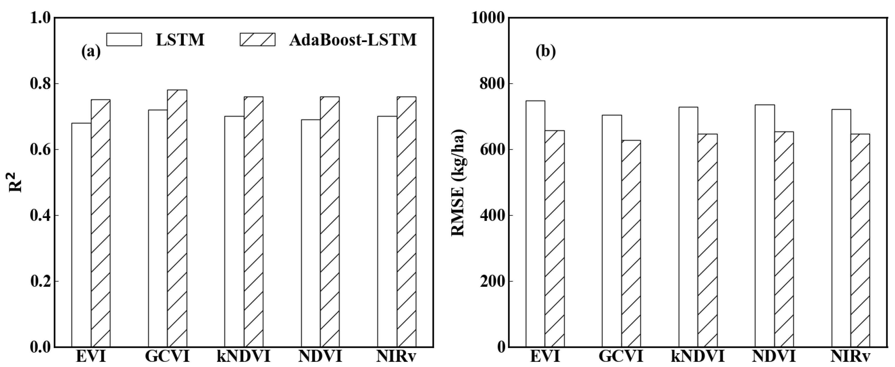
3.2. Performances of Different Yield Prediction Models

Performances of yield prediction models developed by different input characteristic variables and statistical regression algorithms are shown in Figure 6. Among them, the accuracy metrics were generated through the random splitting validation (7:3) using the validation samples (validation data: 2440 samples) from 2001 to 2020. The performance of the yield prediction model developed with the GCVI and meteorological data (R2 ranged from 0.72 to 0.78, RMSE ranged from 627 kg/ha to 703 kg/ha) was better than that developed with other VIs and meteorological data (R2 ranged from 0.68 to 0.76, RMSE ranged from 646 kg/ha to 747.8 kg/ha) (Figure 6). The GCVI has more advantages in predicting yield compared with other VIs.
The AdaBoost-LSTM model developed in this study had the best performance compared with the LSTM model. The R2 and RMSE values of the AdaBoost-LSTM model based on multi-source input data (including the GCVI and meteorological data) reached 0.78 and 627 kg/ha, respectively, which indicated that the AdaBoost-LSTM model has a good application prospect in yield prediction on a regional scale.

3.3. Performance of the Optimal Model under Different Irrigation and Extreme Weather Events

The meteorological conditions in the HHHP during 2001–2020 are shown in Figure 7. According to Figure 7, low temperature events in 2003, 2005, 2010, 2011 and 2013, drought events in 2010 and high temperature events in 2007, 2017 and 2020 were relatively severe. Therefore, these years were defined as extreme years, and the other years were defined as normal years.
The “leave-one-year-out” method was used to test the performance of the AdaBoost-LSTM model under different irrigation and meteorological conditions. As is shown in Figure 8, the AdaBoost-LSTM model generally performed better in rainfed (R2 was 0.73, RMSE was 639 kg/ha) and irrigation (R2 was 63, RMSE was 635.1 kg/ha) counties in all years. In normal years, the accuracy of the AdaBoost-LSTM model in rainfed counties was higher than that in irrigation counties. Relatively speaking, the error of AdaBoost-LSTM model in irrigation counties was lower than that in rainfed counties in extreme years. In general, the AdaBoost-LSTM model can achieve acceptable predictions under different irrigation and extreme weather events.

3.4. The Optimal Prediction Window for Wheat Yield Prediction in the HHHP

Performances of the AdaBoost-LSTM model combined with input characteristic variables of different growth periods from 2001 to 2020 indicated that the performances were significantly improved with the accumulation of input characteristic variables at multiple growth periods (Figure 9). The R2 values for the prediction model only developed with characteristic variables in October was 0.35. The performance for the prediction model developed with characteristic variables from October to the following February was improved, but R2 was still lower than 0.62. During the above period, wheat was in the early growth period, and meteorological variables played an important role in the yield prediction model, such as Tmin in December, Tmax in January and Pr in February (Figure 10). However, the spatial difference of VIs was insignificant, and the ability to reflect the space information was poor, which affected the accuracy of the yield prediction model. Wheat growth accelerated with the rise in temperature in February, and the spatial information reflected by the GCVI greatly increased, and the importance of the GCVI in April and May increased significantly (Figure 10a). The prediction ability of models developed with characteristic variables in the prediction window from October to the following April or May was further improved, while the R2 held steady above 0.76. However, considering the large amount of data processing in large-scale regions, shortening of the prediction window and reduction of data demand must be noted. In summary, the yield prediction model developed with characteristic variables of the prediction window from February to April (roughly from GD to HD) had similar prediction accuracy and small data demand and can achieve the yield prediction in one to two months of lead time before maturity, which is the optimal prediction window.

4. Discussion

Due to the lack of a classification map of specific crops, the crop yield prediction model in some studies was developed using the cropland map as mask data to mask input variables such as satellite images and climate data [11,49,75]. This often led to the confusion between target crop and other crops and increased the uncertainty of the crop yield prediction model, though these studies achieved the target of yield prediction to a certain extent. The classification maps of specific crops (e.g., maize and rice) at 1 km resolution were used as mask data to develop yield prediction models in some studies [35,76]. However, crop maps at coarse resolution were affected by mixed pixels, and input variables masked based on this data would have a large deviation compared with the standard observations. Therefore, relatively accurate crop maps at high resolution can reduce errors in RS data and climate data masked by crop maps and can further improve the model prediction precision [77]. In this study, the wheat planting area at 30 m resolution was extracted in the HHHP, which reduced the impact of mixed pixels on the yield prediction to some extent.
The response of crop growth to external environmental conditions was nonlinear because of the complexity in the crop growth system. ML models can explore the effective information of multi-source and multidimensional datasets, reduce the error of prediction and have great potential for crop yield prediction in a large-scale region [49,71]. In addition, compared with a single model, the ensemble model can further reduce the error of the prediction model and improve the model performance [26,27,28]. In this study, as compared with the LSTM model, the AdaBoost-LSTM model combined with the AdaBoost and LSTM algorithm had the highest accuracy and robustness in wheat yield prediction. However, a lack of training samples led to a large deviation for the prediction in high-yield and low-yield counties, which increased the uncertainty of prediction model [19]. In the future, the data-processing ability of ML algorithms can function at full capacity by obtaining more sample data, and the accuracy and robustness of the prediction model can be improved.
VIs had different performances in crop yield prediction [41]. The emerging VIs (e.g., kNDVI and NIRv) had good performance in the evaluation of plant traits and GPP [39,43,78]. Performances of the emerging and traditional VIs were systematically compared in this study in the prediction of crop yield. The results of this study showed that the prediction model developed with the GCVI outperformed models developed with other VIs, including the NDVI, EVI, kNDVI and NIRv. There was a significant correlation between the GCVI and the LAI, and the GCVI can improve the sensitivity to high biomass compared with the NDVI [45,79]. Therefore, the GCVI was used as the yield predictor for multiple crops in many previous studies [51,80,81].
Irrigation and rainfed agriculture coexisted, and agricultural management measures were very complicated in the HHHP [82]. The irrigation measures will be different according to conditions and the subjective judgment of farmers [83,84], which will increase the uncertainty of crop yield prediction. The accuracy of yield prediction in irrigation and rainfed agriculture was quite different [8]. However, the yield prediction model developed by combining the ensemble model and multi-source data in this study obtained acceptable accuracy in both irrigation and rainfed counties (R2 was between 0.63 and 0.73, RMSE was between 635.1 kg/ha and 639 kg/ha), and the difference in model performance for irrigation and rainfed agriculture was not prominent.
Extreme temperature and drought stress had adverse effects on crop growth and yield formation [50,85], which will affect the accuracy of yield prediction. Cai et al. [14] showed that their prediction model had low performance for predicting wheat yield in Australia in 2006 with extreme drought. Jiang et al. [49] found that the error of the LSTM model for predicting corn yield in the US Corn Belt under extreme weather events is higher than that in normal years. In this study, the AdaBoost-LSTM model had strong robustness for predicting wheat yield in normal years (R2 was 0.73, RMSE was 638 kg/ha) and extreme years (R2 was 0.71, RMSE was 633.9 kg/ha) generally.
The performance of the yield prediction model combined with input variables at different growth periods exhibited great differences. This was mainly because input characteristic variables at different periods have different levels of importance in the yield prediction model [15]. A suitable prediction time window can not only obtain excellent yield prediction but can also reduce the need for training data. The importance of RS information, such as Vis, in the yield prediction model was significantly lower than that of climate variables in the early growth periods for wheat, while VIs can reflect more information about crop growth, and its importance in yield prediction model increased rapidly after entering the peak growth period [14,86]. In this study, meteorological variables (e.g., Tmin in December, Tmax in January and Pr in February) in the early growth stage of wheat were of high importance in the yield prediction model. However, the importance of the VI in the middle and late period of wheat growth (from April to May) was far more important than other input variables and occupied a dominant position. Considering the appropriate shortening of the prediction time window and the reduction in training data demand, the window from February to April was recommended as the best yield prediction time window.
However, there were some limitations to this study. First, the prediction accuracy of the wheat yield using the AdaBoost-LSTM model in irrigation counties was lower than that in rainfed counties in most years. Obtaining the dataset about irrigation management practices may be a way to improve the model prediction performance in irrigation counties. On the other hand, using the AdaBoost-LSTM model to obtain high-resolution crop yield maps in large-scale areas also faces the challenge of computational efficiency. In the future, with more input variables and further improvement of the AdaBoost-LSTM model, the model will have great potential in crop yield prediction.

5. Conclusions

In this study, AdaBoost-LSTM was developed to predict wheat yield based on multi-source data, such as VIs and meteorological data. The results showed that the GCVI is the optimal RS variable for wheat yield prediction compared with other VIs (including emerging VIs). Compared with the LSTM model, the AdaBoost-LSTM model had the best performance. In general, the AdaBoost-LSTM model with the GCVI as input data had strong robustness for predicting wheat yield in irrigation and rainfed counties in extreme years. The window from February to April was the best prediction time window for wheat yield prediction, which can realize the yield prediction with one to two months of lead time before maturity with less input data. The results can provide a method of support for large-scale regional crop yield prediction. However, the structure of the AdaBoost-LSTM model was more complex, resulting in a large amount of calculation, and it was difficult to apply in a large number of pixels. In the future, we hope to obtain high spatial-resolution crop yield maps by simplifying or improving the AdaBoost-LSTM model.

Author Contributions

Conceptualization, methodology, software, validation, formal analysis, investigation, writing—original draft, Y.Z. (Yanxi Zhao); conceptualization, methodology, software, validation, formal analysis, J.H.; writing—review and editing, visualization, funding acquisition, Y.T., X.Y., T.C., Y.Z. (Yan Zhu) and W.C. All authors have read and agreed to the published version of the manuscript.

Funding

This work was supported by the National Natural Science Foundation of China (No. 32371990), the Innovative Research Group Project of the National Natural Science Foundation of China (32021004) and Jiangsu Provincial Key R&D plan (BE2023368).

Data Availability Statement

Data will be made available upon request.

Conflicts of Interest

The authors declare no conflicts of interest.

References

  1. Kong, X.; Lal, R.; Li, B.; Liu, H.; Li, K.; Feng, G.; Zhang, Q.; Zhang, B. Fertilizer Intensification and Its Impacts in China’s HHH Plains. In Advances in Agronomy; Sparks, D.L., Ed.; Academic Press: Cambridge, MA, USA, 2014; Volume 125, pp. 135–169. [Google Scholar]
  2. Becker-Reshef, I.; Vermote, E.; Lindeman, M.; Justice, C. A generalized regression-based model for forecasting winter wheat yields in Kansas and Ukraine using MODIS data. Remote Sens. Environ. 2010, 114, 1312–1323. [Google Scholar] [CrossRef]
  3. Tao, F.; Zhang, L.; Zhang, Z.; Chen, Y. Designing wheat cultivar adaptation to future climate change across China by coupling biophysical modelling and machine learning. Eur. J. Agron. 2022, 136, 126500. [Google Scholar] [CrossRef]
  4. Vintrou, E.; Desbrosse, A.; Bégué, A.; Traoré, S.; Baron, C.; Lo Seen, D. Crop area mapping in West Africa using landscape stratification of MODIS time series and comparison with existing global land products. Int. J. Appl. Earth. Obs. 2012, 14, 83–93. [Google Scholar] [CrossRef]
  5. Benami, E.; Jin, Z.; Carter, M.R.; Ghosh, A.; Hijmans, R.J.; Hobbs, A.; Kenduiywo, B.; Lobell, D.B. Uniting remote sensing, crop modelling and economics for agricultural risk management. Nat. Rev. Earth Environ. 2021, 2, 140–159. [Google Scholar] [CrossRef]
  6. Zhou, K.; Cao, L.; Shen, X.; Wang, G. Novel spectral indices for enhanced estimations of 3-dimentional flavonoid contents for Ginkgo plantations using UAV-borne LiDAR and hyperspectral data. Remote Sens. Environ. 2023, 299, 113882. [Google Scholar] [CrossRef]
  7. Satir, O.; Berberoglu, S. Crop yield prediction under soil salinity using satellite derived vegetation indices. Field Crops Res. 2016, 192, 134–143. [Google Scholar] [CrossRef]
  8. Jeffries, G.R.; Griffin, T.S.; Fleisher, D.H.; Naumova, E.N.; Koch, M.; Wardlow, B.D. Mapping sub-field maize yields in Nebraska, USA by combining remote sensing imagery, crop simulation models, and machine learning. Precis. Agric. 2019, 21, 678–694. [Google Scholar] [CrossRef]
  9. Feng, P.; Wang, B.; Liu, D.L.; Waters, C.; Yu, Q. Incorporating machine learning with biophysical model can improve the evaluation of climate extremes impacts on wheat yield in south-eastern Australia. Agric. For. Meteorol. 2019, 275, 100–113. [Google Scholar] [CrossRef]
  10. Li, Y.; Guan, K.; Yu, A.; Peng, B.; Zhao, L.; Li, B.; Peng, J. Toward building a transparent statistical model for improving crop yield prediction: Modeling rainfed corn in the U.S. Field Crops Res. 2019, 234, 55–65. [Google Scholar] [CrossRef]
  11. Kamir, E.; Waldner, F.; Hochman, Z. Estimating wheat yields in Australia using climate records, satellite image time series and machine learning methods. ISPRS. J. Photogramm. 2020, 160, 124–135. [Google Scholar] [CrossRef]
  12. Oliveira, R.A.; Näsi, R.; Niemeläinen, O.; Nyholm, L.; Honkavaara, E. Machine learning estimators for the quantity and quality of grass swards used for silage production using drone-based imaging spectrometry and photogrammetry. Remote Sens. Environ. 2020, 246, 111830. [Google Scholar] [CrossRef]
  13. Feng, P.; Wang, B.; Liu, D.L.; Waters, C.; Xiao, D.; Shi, L.; Yu, Q. Dynamic wheat yield forecasts are improved by a hybrid approach using a biophysical model and machine learning technique. Agric. For. Meteorol. 2020, 285–286, 107922. [Google Scholar] [CrossRef]
  14. Cai, Y.; Guan, K.; Lobell, D.; Potgieter, A.B.; Wang, S.; Peng, J.; Xu, T.; Asseng, S.; Zhang, Y.; You, L.; et al. Integrating satellite and climate data to predict wheat yield in Australia using machine learning approaches. Agric. For. Meteorol. 2019, 274, 144–159. [Google Scholar] [CrossRef]
  15. Han, J.; Zhang, Z.; Cao, J.; Luo, Y.; Zhang, L.; Li, Z.; Zhang, J. Prediction of winter wheat yield based on multi-source data and machine learning in China. Remote Sens. 2020, 12, 236. [Google Scholar] [CrossRef]
  16. Cai, Y.; Guan, K.; Peng, J.; Wang, S.; Seifert, C.; Wardlow, B.; Li, Z. A high-performance and in-season classification system of field-level crop types using time-series Landsat data and a machine learning approach. Remote Sens. Environ. 2018, 210, 35–47. [Google Scholar] [CrossRef]
  17. LeCun, Y.; Bengio, Y.; Hinton, G. Deep learning. Nature 2015, 521, 436–444. [Google Scholar] [CrossRef] [PubMed]
  18. Khaki, S.; Pham, H.; Wang, L. Simultaneous corn and soybean yield prediction from remote sensing data using deep transfer learning. Sci. Rep. 2021, 11, 11132. [Google Scholar] [CrossRef] [PubMed]
  19. Ma, Y.; Zhang, Z.; Kang, Y.; Özdoğan, M. Corn yield prediction and uncertainty analysis based on remotely sensed variables using a Bayesian neural network approach. Remote Sens. Environ. 2021, 259, 112408. [Google Scholar] [CrossRef]
  20. Tian, H.; Wang, P.; Tansey, K.; Zhang, J.; Zhang, S.; Li, H. An LSTM neural network for improving wheat yield estimates by integrating remote sensing data and meteorological data in the Guanzhong Plain, PR China. Agric. For. Meteorol. 2021, 310, 108629. [Google Scholar] [CrossRef]
  21. Zhang, L.; Zhang, Z.; Luo, Y.; Cao, J.; Xie, R.; Li, S. Integrating satellite-derived climatic and vegetation indices to predict smallholder maize yield using deep learning. Agric. For. Meteorol. 2021, 311, 108666. [Google Scholar] [CrossRef]
  22. Feng, L.; Zhang, Z.; Ma, Y.; Du, Q.; Williams, P.; Drewry, J.; Luck, B. Alfalfa Yield Prediction Using UAV-Based Hyperspectral Imagery and Ensemble Learning. Remote Sens. 2020, 12, 2028. [Google Scholar] [CrossRef]
  23. Fu, B.; He, X.; Yao, H.; Liang, Y.; Deng, T.; He, H.; Fan, D.; Lan, G.; He, W. Comparison of RFE-DL and stacking ensemble learning algorithms for classifying mangrove species on UAV multispectral images. Int. J. Appl. Earth Obs. 2022, 112, 102890. [Google Scholar] [CrossRef]
  24. Long, X.; Li, X.; Lin, H.; Zhang, M. Mapping the vegetation distribution and dynamics of a wetland using adaptive-stacking and Google Earth Engine based on multi-source remote sensing data. Int. J. Appl. Earth. Obs. 2021, 102, 102453. [Google Scholar] [CrossRef]
  25. Ma, J.-W.; Nguyen, C.-H.; Lee, K.; Heo, J. Regional-scale rice-yield estimation using stacked auto-encoder with climatic and MODIS data: A case study of South Korea. Int. J. Remote Sens. 2019, 40, 51–71. [Google Scholar] [CrossRef]
  26. Feng, L.; Li, Y.; Wang, Y.; Du, Q. Estimating hourly and continuous ground-level PM2.5 concentrations using an ensemble learning algorithm: The ST-stacking model. Atmos. Environ. 2020, 223, 117242. [Google Scholar] [CrossRef]
  27. Jiang, Z.; Yang, S.; Smith, P.; Pang, Q. Ensemble machine learning for modeling greenhouse gas emissions at different time scales from irrigated paddy fields. Field Crops Res. 2023, 292, 108821. [Google Scholar] [CrossRef]
  28. Su, B.; Huang, J.; Mondal, S.K.; Zhai, J.; Wang, Y.; Wen, S.; Gao, M.; Lv, Y.; Jiang, S.; Jiang, T.; et al. Insight from CMIP6 SSP-RCP scenarios for future drought characteristics in China. Atmos. Res. 2021, 250, 105375. [Google Scholar] [CrossRef]
  29. Yu, W.; Yang, G.; Li, D.; Zheng, H.; Yao, X.; Zhu, Y.; Cao, W.; Qiu, L.; Cheng, T. Improved prediction of rice yield at field and county levels by synergistic use of SAR, optical and meteorological data. Agric. For. Meteorol. 2023, 342, 109729. [Google Scholar] [CrossRef]
  30. Li, M.; Zhao, J.; Yang, X. Building a new machine learning-based model to estimate county-level climatic yield variation for maize in Northeast China. Comput. Electron. Agric. 2021, 191, 106557. [Google Scholar] [CrossRef]
  31. Freund, Y.; Schapire, R.E. A Decision-Theoretic Generalization of On-Line Learning and an Application to Boosting. J. Comput. Syst. Sci. 1997, 55, 119–139. [Google Scholar] [CrossRef]
  32. Hu, D.; Zhang, C.; Cao, W.; Lv, X.; Xie, S. Grain Yield Predict Based on GRA-AdaBoost-SVR Model. J. Big Data 2021, 3, 65–76. [Google Scholar] [CrossRef]
  33. Sun, S.; Wei, Y.; Wang, S. AdaBoost-LSTM Ensemble Learning for Financial Time Series Forecasting. In Computational Science–ICCS 2018; Shi, Y., Fu, H., Tian, Y., Krzhizhanovskaya, V.V., Lees, M.H., Dongarra, J., Sloot, P.M.A., Eds.; Springer International Publishing: Cham, Switzerland, 2018; pp. 590–597. [Google Scholar]
  34. Son, N.T.; Chen, C.F.; Chen, C.R.; Minh, V.Q.; Trung, N.H. A comparative analysis of multitemporal MODIS EVI and NDVI data for large-scale rice yield estimation. Agric. For. Meteorol. 2014, 197, 52–64. [Google Scholar] [CrossRef]
  35. Cao, J.; Zhang, Z.; Tao, F.; Zhang, L.; Luo, Y.; Zhang, J.; Han, J.; Xie, J. Integrating multi-source data for rice yield prediction across China using machine learning and deep learning approaches. Agric. For. Meteorol. 2021, 297, 108275. [Google Scholar] [CrossRef]
  36. Li, Z.; Ding, L.; Xu, D. Exploring the potential role of environmental and multi-source satellite data in crop yield prediction across Northeast China. Sci. Total Environ. 2022, 815, 152880. [Google Scholar] [CrossRef]
  37. Zhou, W.; Liu, Y.; Ata-Ul-Karim, S.T.; Ge, Q.; Li, X.; Xiao, J. Integrating climate and satellite remote sensing data for predicting county-level wheat yield in China using machine learning methods. Int. J. Appl. Earth Obs. Geoinf. 2022, 111, 102861. [Google Scholar] [CrossRef]
  38. Guan, K.; Berry, J.A.; Zhang, Y.; Joiner, J.; Guanter, L.; Badgley, G.; Lobell, D.B. Improving the monitoring of crop productivity using spaceborne solar-induced fluorescence. Glob. Change Biol. 2016, 22, 716–726. [Google Scholar] [CrossRef]
  39. Badgley, G.; Field, C.B.; Berry, J.A. Canopy near-infrared reflectance and terrestrial photosynthesis. Sci. Adv. 2017, 3, e1602244. [Google Scholar] [CrossRef]
  40. Wang, S.; Zhang, Y.; Ju, W.; Qiu, B.; Zhang, Z. Tracking the seasonal and inter-annual variations of global gross primary production during last four decades using satellite near-infrared reflectance data. Sci. Total Environ. 2021, 755, 142569. [Google Scholar] [CrossRef]
  41. Li, L.; Wang, B.; Feng, P.; Li Liu, D.; He, Q.; Zhang, Y.; Wang, Y.; Li, S.; Lu, X.; Yue, C.; et al. Developing machine learning models with multi-source environmental data to predict wheat yield in China. Comput. Electron. Agric. 2022, 194, 106790. [Google Scholar] [CrossRef]
  42. Zhang, J.; Xiao, J.; Tong, X.; Zhang, J.; Meng, P.; Li, J.; Liu, P.; Yu, P. NIRv and SIF better estimate phenology than NDVI and EVI: Effects of spring and autumn phenology on ecosystem production of planted forests. Agric. For. Meteorol. 2022, 315, 108819. [Google Scholar] [CrossRef]
  43. Camps-Valls, G.; Campos-Taberner, M.; Moreno-Martínez, Á.; Walther, S.; Duveiller, G.; Cescatti, A.; Mahecha, M.D.; Muñoz-Marí, J.; García-Haro, F.J.; Guanter, L.; et al. A unified vegetation index for quantifying the terrestrial biosphere. Sci. Adv. 2021, 7, eabc7447. [Google Scholar] [CrossRef]
  44. Gitelson, A.A.; Viña, A.; Arkebauer, T.J.; Rundquist, D.C.; Keydan, G.; Leavitt, B. Remote estimation of leaf area index and green leaf biomass in maize canopies. Geophys. Res. Lett. 2003, 30, 1248. [Google Scholar] [CrossRef]
  45. Nguy-Robertson, A.; Gitelson, A.; Peng, Y.; Viña, A.; Arkebauer, T.; Rundquist, D. Green leaf area index estimation in maize and soybean: Combining vegetation indices to achieve maximal sensitivity. Agron. J. 2012, 104, 1336–1347. [Google Scholar] [CrossRef]
  46. Pan, Y.; Li, L.; Zhang, J.; Liang, S.; Zhu, X.; Sulla-Menashe, D. Winter wheat area estimation from MODIS-EVI time series data using the Crop Proportion Phenology Index. Remote Sens. Environ. 2012, 119, 232–242. [Google Scholar] [CrossRef]
  47. Luo, Y.; Zhang, Z.; Li, Z.; Chen, Y.; Zhang, L.; Cao, J.; Tao, F. Identifying the spatiotemporal changes of annual harvesting areas for three staple crops in China by integrating multi-data sources. Environ. Res. Lett. 2020, 15, 074003. [Google Scholar] [CrossRef]
  48. Yang, G.; Yu, W.; Yao, X.; Zheng, H.; Cao, Q.; Zhu, Y.; Cao, W.; Cheng, T. AGTOC: A novel approach to winter wheat mapping by automatic generation of training samples and one-class classification on Google Earth Engine. Int. J. Appl. Earth. Obs. 2021, 102, 102446. [Google Scholar] [CrossRef]
  49. Jiang, H.; Hu, H.; Zhong, R.; Xu, J.; Xu, J.; Huang, J.; Wang, S.; Ying, Y.; Lin, T. A deep learning approach to conflating heterogeneous geospatial data for corn yield estimation: A case study of the US Corn Belt at the county level. Glob. Change Biol. 2020, 26, 1754–1766. [Google Scholar] [CrossRef] [PubMed]
  50. Lobell, D.B.; Deines, J.M.; Tommaso, S.D. Changes in the drought sensitivity of US maize yields. Nat. Food. 2020, 1, 729–735. [Google Scholar] [CrossRef] [PubMed]
  51. Zhao, Y.; Tao, H.; He, P.; Yao, X.; Cheng, T.; Zhu, Y.; Cao, W.; Tian, Y. Annual 30 m winter wheat yield mapping in the Huang-Huai-Hai plain using crop growth model and long-term satellite images. Comput. Electron. Agric. 2023, 214, 108335. [Google Scholar] [CrossRef]
  52. Huang, H.; Chen, Y.; Clinton, N.; Wang, J.; Wang, X.; Liu, C.; Gong, P.; Yang, J.; Bai, Y.; Zheng, Y.; et al. Mapping major land cover dynamics in Beijing using all Landsat images in Google Earth Engine. Remote Sens. Environ. 2017, 202, 166–176. [Google Scholar] [CrossRef]
  53. Liu, X.; Hu, G.; Chen, Y.; Li, X.; Xu, X.; Li, S.; Pei, F.; Wang, S. High-resolution multi-temporal mapping of global urban land using Landsat images based on the Google Earth Engine Platform. Remote Sens. Environ. 2018, 209, 227–239. [Google Scholar] [CrossRef]
  54. Tucker, C.J. Red and photographic infrared linear combinations for monitoring vegetation. Remote Sens. Environ. 1979, 8, 127–150. [Google Scholar] [CrossRef]
  55. Teluguntla, P.; Thenkabail, P.S.; Oliphant, A.; Xiong, J.; Gumma, M.K.; Congalton, R.G.; Yadav, K.; Huete, A. A 30-m landsat-derived cropland extent product of Australia and China using random forest machine learning algorithm on Google Earth Engine cloud computing platform. ISPRS. J. Photogramm. 2018, 144, 325–340. [Google Scholar] [CrossRef]
  56. Zhang, Y.; Qi, Y.; Shen, Y.; Wang, H.; Pan, X. Mapping the agricultural land use of the North China plain in 2002 and 2012. J. Geogr. Sci. 2019, 29, 909–921. [Google Scholar] [CrossRef]
  57. Zha, Y.; Ni, S.; Yang, S. An effective approach to automatically extract urban land-use from TM imagery. J. Remote Sens. 2003, 7, 37–41. [Google Scholar]
  58. Xu, H. A study on information extraction of water body with the modified normalized difference water index (MNDWI). J. Remote Sens. 2005, 9, 589–595. [Google Scholar]
  59. Li, K.; Chen, Y. A genetic algorithm-based urban cluster automatic threshold method by combining VIIRS DNB, NDVI, and NDBI to monitor urbanization. Remote Sens. 2018, 10, 277. [Google Scholar] [CrossRef]
  60. Titolo, A. Use of Time-Series NDWI to Monitor Emerging Archaeological Sites: Case Studies from Iraqi Artificial Reservoirs. Remote Sens. 2021, 13, 786. [Google Scholar] [CrossRef]
  61. Abatzoglou, J.T.; Dobrowski, S.Z.; Parks, S.A.; Hegewisch, K.C. TerraClimate, a high-resolution global dataset of monthly climate and climatic water balance from 1958–2015. Sci. Data 2018, 5, 170191. [Google Scholar] [CrossRef]
  62. Bushong, J.T.; Mullock, J.L.; Miller, E.C.; Raun, W.R.; Klatt, A.R.; Arnall, D.B. Development of an in-season estimate of yield potential utilizing optical crop sensors and soil moisture data for winter wheat. Precis. Agric. 2016, 17, 451–469. [Google Scholar] [CrossRef]
  63. Babaeian, E.; Paheding, S.; Siddique, N.; Devabhaktuni, V.K.; Tuller, M. Estimation of root zone soil moisture from ground and remotely sensed soil information with multisensor data fusion and automated machine learning. Remote Sens. Environ. 2021, 260, 112434. [Google Scholar] [CrossRef]
  64. Fang, Q.; Wang, Y.; Uwimpaye, F.; Yan, Z.; Li, L.; Liu, X.; Shao, L. Pre-sowing soil water conditions and water conservation measures affecting the yield and water productivity of summer maize. Agric. Water Manag. 2021, 245, 106628. [Google Scholar] [CrossRef]
  65. Jonsson, P.; Eklundh, L. Seasonality extraction by function fitting to time-series of satellite sensor data. IEEE Trans. Geosci. Remote Sens. 2002, 40, 1824–1832. [Google Scholar] [CrossRef]
  66. Wu, W.; Yang, P.; Tang, H.; Shibasaki, R.; Zhou, Q.; Zhang, L. Monitoring spatial patterns of cropland phenology in North China based on NOAA NDVI data. Sci. Agric. Sin. 2009, 42, 552–560. [Google Scholar]
  67. Luo, Y.; Zhang, Z.; Chen, Y.; Li, Z.; Tao, F. ChinaCropPhen1km: A high-resolution crop phenological dataset for three staple crops in China during 2000–2015 based on leaf area index (LAI) products. Earth Syst. Sci. Data 2020, 12, 197–214. [Google Scholar] [CrossRef]
  68. Sakamoto, T.; Wardlow, B.D.; Gitelson, A.A.; Verma, S.B.; Suyker, A.E.; Arkebauer, T.J. A Two-Step Filtering approach for detecting maize and soybean phenology with time-series MODIS data. Remote Sens. Environ. 2010, 114, 2146–2159. [Google Scholar] [CrossRef]
  69. Carrasco, L.; Fujita, G.; Kito, K.; Miyashita, T. Historical mapping of rice fields in Japan using phenology and temporally aggregated Landsat images in Google Earth Engine. ISPRS. J. Photogramm. 2022, 191, 277–289. [Google Scholar] [CrossRef]
  70. Breiman, L. Random forest. Mach. Learn. 2001, 45, 5–32. [Google Scholar] [CrossRef]
  71. Hunt, M.L.; Blackburn, G.A.; Carrasco, L.; Redhead, J.W.; Rowland, C.S. High resolution wheat yield mapping using Sentinel-2. Remote Sens. Environ. 2019, 233, 111410. [Google Scholar] [CrossRef]
  72. Hochreiter, S.; Schmidhuber, J. Long Short-Term Memory. Neural Comput. 1997, 9, 1735–1780. [Google Scholar] [CrossRef]
  73. Song, X.-P.; Li, H.; Potapov, P.; Hansen, M.C. Annual 30 m soybean yield mapping in Brazil using long-term satellite observations, climate data and machine learning. Agric. For. Meteorol. 2022, 326, 109186. [Google Scholar] [CrossRef]
  74. Cao, J.; Zhang, Z.; Luo, Y.; Zhang, L.; Zhang, J.; Li, Z.; Tao, F. Wheat yield predictions at a county and field scale with deep learning, machine learning, and google earth engine. Eur. J. Agron. 2021, 123, 126204. [Google Scholar] [CrossRef]
  75. Johnson, D.M. An assessment of pre- and within-season remotely sensed variables for forecasting corn and soybean yields in the United States. Remote Sens. Environ. 2014, 141, 116–128. [Google Scholar] [CrossRef]
  76. Zhang, L.; Zhang, Z.; Luo, Y.; Cao, J.; Tao, F. Combining optical, fluorescence, thermal satellite, and environmental data to predict county-level maize yield in China using machine learning approaches. Remote Sens. 2020, 12, 21. [Google Scholar] [CrossRef]
  77. Guan, K.; Li, Z.; Rao, L.N.; Gao, F.; Xie, D.; Hien, N.T.; Zeng, Z. Mapping paddy rice area and yields over Thai Binh province in Viet Nam from MODIS, Landsat, and ALOS-2/PALSAR-2. IEEE J.-Stars 2018, 11, 2238–2252. [Google Scholar] [CrossRef]
  78. Wang, Q.; Moreno-Martínez, Á.; Muñoz-Marí, J.; Campos-Taberner, M.; Camps-Valls, G. Estimation of vegetation traits with kernel NDVI. ISPRS. J. Photogramm. 2023, 195, 408–417. [Google Scholar] [CrossRef]
  79. Lobell, D.B.; Thau, D.; Seifert, C.; Engle, E.; Little, B. A scalable satellite-based crop yield mapper. Remote Sens. Environ. 2015, 164, 324–333. [Google Scholar] [CrossRef]
  80. Azzari, G.; Jain, M.; Lobell, D.B. Towards fine resolution global maps of crop yields: Testing multiple methods and satellites in three countries. Remote Sens. Environ. 2017, 202, 129–141. [Google Scholar] [CrossRef]
  81. Jin, Z.; Azzari, G.; Lobell, D.B. Improving the accuracy of satellite-based high-resolution yield estimation: A test of multiple scalable approaches. Agric. For. Meteorol. 2017, 247, 207–220. [Google Scholar] [CrossRef]
  82. Xiao, L.; Wang, G.; Zhou, H.; Jin, X.; Luo, Z. Coupling agricultural system models with machine learning to facilitate regional predictions of management practices and crop production. Environ. Res. Lett. 2022, 17, 114027. [Google Scholar] [CrossRef]
  83. Ren, C.; Zhou, X.; Wang, C.; Guo, Y.; Diao, Y.; Shen, S.; Reis, S.; Li, W.; Xu, J.; Gu, B. Ageing threatens sustainability of smallholder farming in China. Nature 2023, 616, 96–103. [Google Scholar] [CrossRef] [PubMed]
  84. Wang, H.; Ren, H.; Zhang, L.; Zhao, Y.; Liu, Y.; He, Q.; Li, G.; Han, K.; Zhang, J.; Zhao, B.; et al. A sustainable approach to narrowing the summer maize yield gap experienced by smallholders in the North China Plain. Agric. Syst. 2023, 204, 103541. [Google Scholar] [CrossRef]
  85. Bailey-Serres, J.; Parker, J.E.; Ainsworth, E.A.; Oldroyd, G.E.D.; Schroeder, J.I. Genetic strategies for improving crop yields. Nature 2019, 575, 109–118. [Google Scholar] [CrossRef] [PubMed]
  86. Cao, J.; Zhang, Z.; Tao, F.; Zhang, L.; Luo, Y.; Han, J.; Li, Z. Identifying the contributions of multi-source data for winter wheat yield prediction in China. Remote Sens. 2020, 12, 750. [Google Scholar] [CrossRef]
Figure 1. The study area and boundary of the 427 counties in the HHHP.
Remotesensing 16 01259 g001
Figure 2. Flow chart of the extraction of wheat planting area and the development of yield prediction model.
Remotesensing 16 01259 g002
Figure 3. The technical flowchart of AdaBoost-LSTM ensemble model.
Remotesensing 16 01259 g003
Figure 4. Comparisons of planting area at county level between the estimated and statistical data collected in 2000, 2005, 2010, 2015 and 2020. Red lines are the linear regression fit. Dashed lines represent the 1:1 lines.
Remotesensing 16 01259 g004
Figure 5. (ae) show the spatial patterns of wheat planting area in the HHHP for 2000, 2005, 2010, 2015, 2020; (f,h) are the close-up views of two randomly selected example locations in the wheat map (2020); (g,i) are the corresponding original satellite images from Landsat (2020).
Remotesensing 16 01259 g005
Figure 6. Performances of yield prediction model developed using different combinations of input variables and regression algorithms. Accuracy metrics ((a) R2; (b) RMSE) were generated through the random splitting validation (7:3) using the validation samples (validation data: 2440 samples) from 2001 to 2020.
Remotesensing 16 01259 g006
Figure 7. The meteorological conditions in the HHHP during 2001–2020. (a) Tmax; (b) Tmin; (c) Pr.
Remotesensing 16 01259 g007
Figure 8. Performance of AdaBoost-LSTM model based on GCVI and meteorological data in irrigation and rainfed counties under different meteorological conditions during 2001–2020. Accuracy metrics were generated based on “leave-one-year-out” method. Dashed lines represent the 1:1 lines.
Remotesensing 16 01259 g008
Figure 9. Performances of yield prediction model combined with input variables during different growth periods. Accuracy metrics were generated through the random splitting validation method in which the samples (n = 8132) from 2001 to 2020 were randomly split into 70% for training (n = 5692) and 30% for validation (n = 2440).
Remotesensing 16 01259 g009
Figure 10. The mean importance of important input characteristic variables at different periods based on RF algorithm using random splitting validation data (7:3) from 2001 to 2020.
Remotesensing 16 01259 g010
Table 1. Data used in this study.
DataVariableSource
Satellite dataNDBI,
MNDWI,
NDVI,
EVI,
GCVI,
kNDVI,
NIRv
Landsat5/7/8,
MOD09A1,
MOD09GA
Meteorological dataPr
Srad
Tmin
Tmax
VPD
ET
SM
TerraClimate
Crop dataphenologyChina’s Meteorological Administration
planting areaChina Agricultural Statistical Yearbook
yield
Disclaimer/Publisher’s Note: The statements, opinions and data contained in all publications are solely those of the individual author(s) and contributor(s) and not of MDPI and/or the editor(s). MDPI and/or the editor(s) disclaim responsibility for any injury to people or property resulting from any ideas, methods, instructions or products referred to in the content.

