
Identification of Ecological Sources Using Ecosystem Service Value and Vegetation Productivity Indicators: A Case Study of the Three-River Headwaters Region, Qinghai–Tibetan Plateau, China


Abstract
1. Introduction
2. Study Area and Datasets
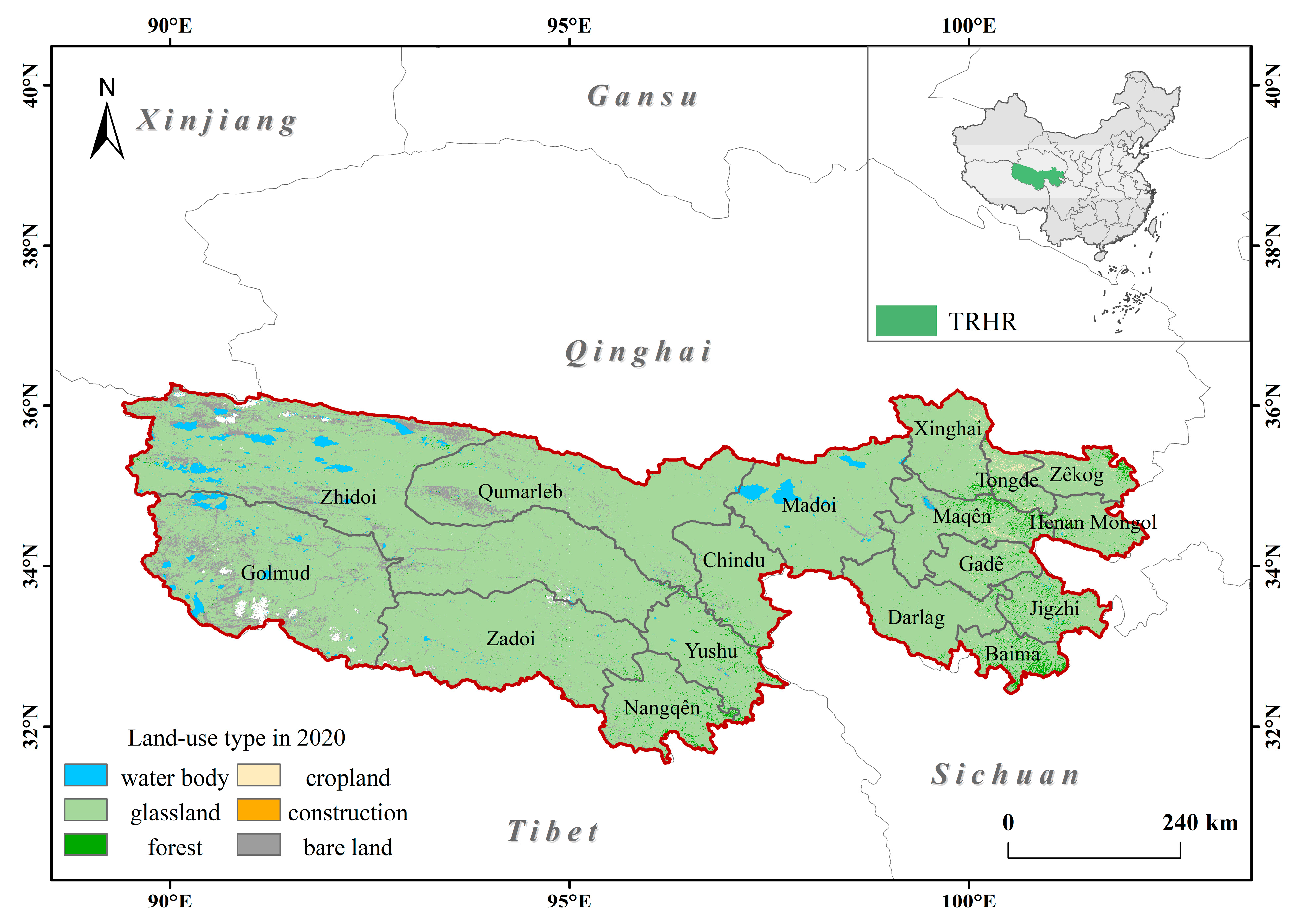
2.1. Study Area
2.2. Data Source and Processing
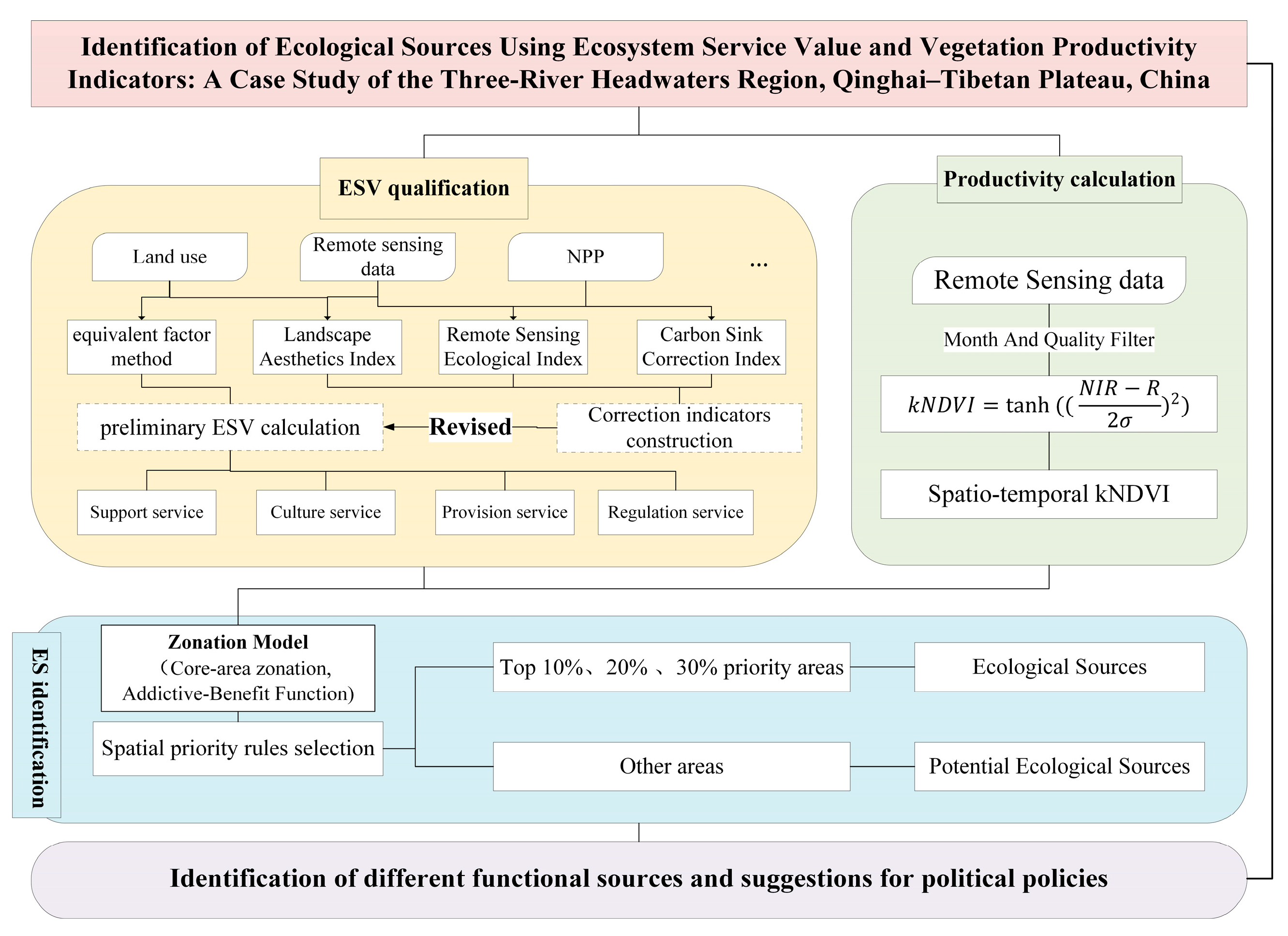
3. Methodology
3.1. Ecosystem Service Value Assessments
3.1.1. Quantification of the Ecosystem Services
3.1.2. Revision of the ESV
3.1.3. Revised ESV Calculation
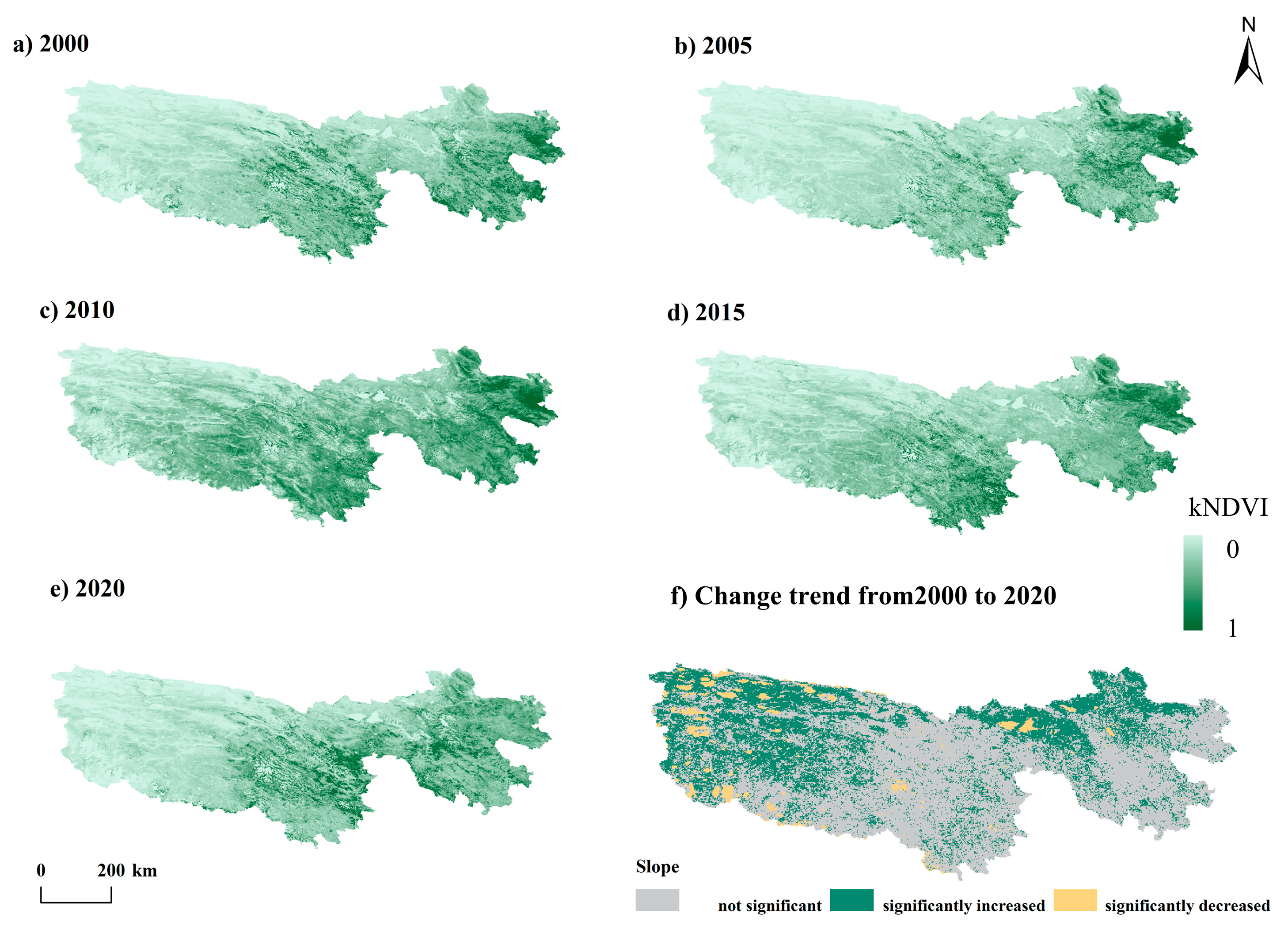
3.2. Kernel Normalized Difference Vegetation Index Calculation
3.3. Ecological Source Identification
4. Results
4.1. ESV and KNDVI of the TRHR Present Significant Spatial Heterogeneity
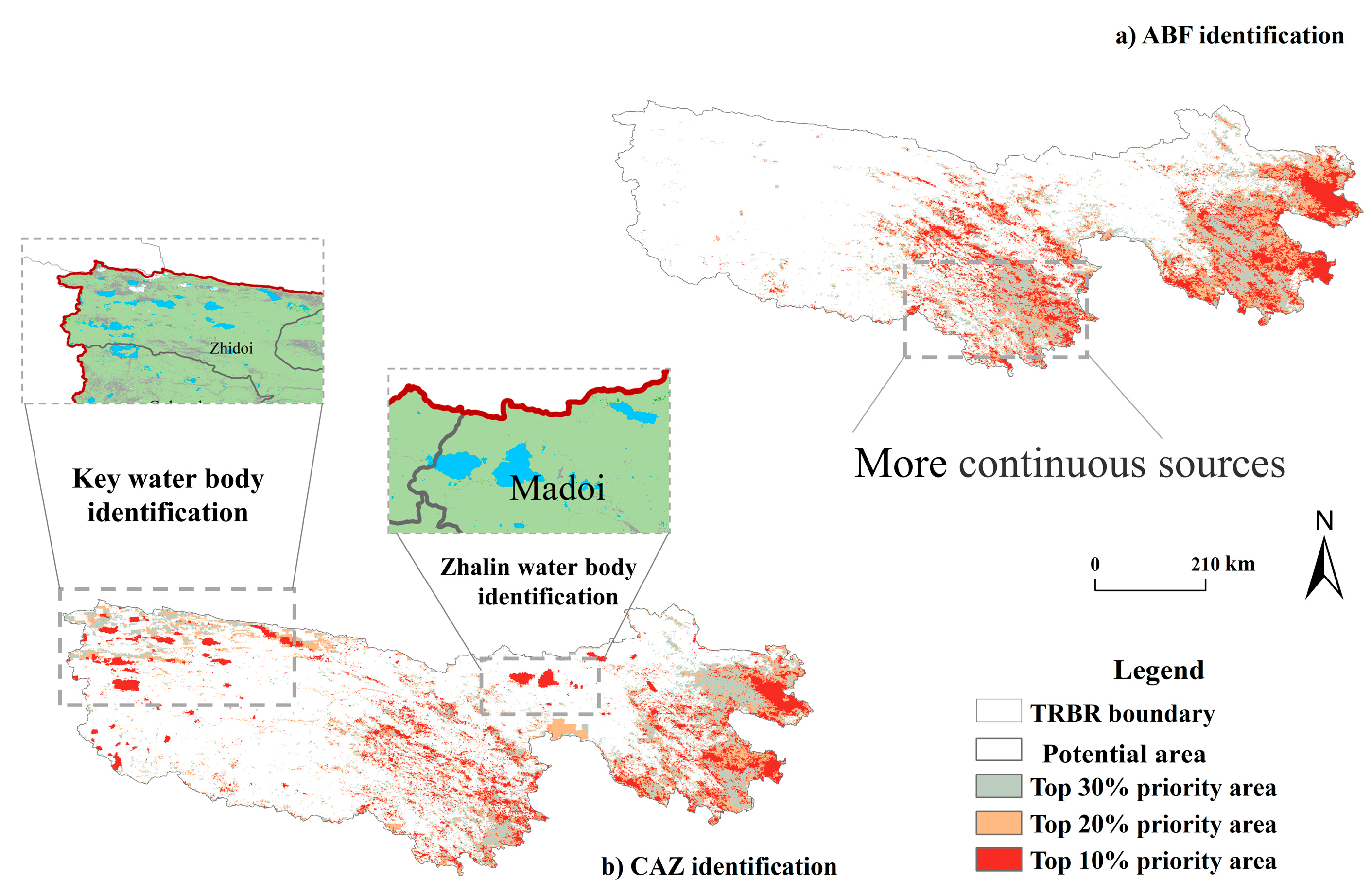
4.2. Ecological Source Identification Model Performance Analysis
5. Discussion
5.1. Implications of the Ecological Source Identification Framework
5.2. Comparison of the Proposed Method and Previous Methods
5.3. Management Implications Based on the Identified Ecological Sources
5.4. Limitations and Future Work
6. Conclusions
Author Contributions
Funding
Data Availability Statement
Acknowledgments
Conflicts of Interest
References
- Fan, S.; Axmacher, J.C.; Shu, H.; Liu, Y. Ecological Network Design Based on Optimizing Ecosystem Services:Case Study in the Huang-Huai-Hai Region, China. Ecol. Indic. 2023, 150, 110264. [Google Scholar] [CrossRef]
- Gu, Z.; Gong, J.; Wang, Y. Construction and Evaluation of Ecological Networks among Natural Protected Areas Based on “Quality-Structure–Function”: A Case Study of the Qinghai-Tibet Area. Ecol. Indic. 2023, 151, 110228. [Google Scholar] [CrossRef]
- Guan, H.; Bai, Y.; Tang, Y.; Zhang, C.; Zou, J. Spatial Identification and Optimization of Ecological Network in Desert-Oasis Area of Yellow River Basin, China. Ecol. Indic. 2023, 147, 109999. [Google Scholar] [CrossRef]
- Dai, L.; Liu, Y.; Luo, X. Integrating the MCR and DOI Models to Construct an Ecological Security Network for the Urban Agglomeration around Poyang Lake, China. Sci. Total Environ. 2021, 754, 141868. [Google Scholar] [CrossRef]
- Tsavdaridou, A.I.; Doxa, A.; Mazaris, A.D. Towards Achieving a Twenty-Fold Increase in the Coverage of Freshwater Species Distributions within Protected Areas in Europe. Biol. Conserv. 2023, 285, 110233. [Google Scholar] [CrossRef]
- Jalkanen, J.; Toivonen, T.; Moilanen, A. Identification of Ecological Networks for Land-Use Planning with Spatial Conservation Prioritization. Landsc. Ecol. 2020, 35, 353–371. [Google Scholar] [CrossRef]
- Wu, W.; Zhao, S.; Guo, J.; Ou, M.; Ding, G. Construction and Optimization of Ecological Security Pattern Based on the Circuit Theory: A Case Study of Hohhot City. Environ. Sci. Pollut. Res. 2023, 30, 89597–89615. [Google Scholar] [CrossRef]
- Jin, L.; Xu, Q.; Yi, J.; Zhong, X. Integrating CVOR-GWLR-Circuit Model into Construction of Ecological Security Pattern in Yunnan Province, China. Environ. Sci. Pollut. Res. 2022, 29, 81520–81545. [Google Scholar] [CrossRef] [PubMed]
- Zhang, D.; Ren, H.; Sun, P.; Jing, P.; Guo, B. Construction of Multi-Level Ecological Security Network in Fragmented Nature Landscape Using the Three-Dimensional Framework of Ecological Adaptability. Ecol. Indic. 2023, 157, 111229. [Google Scholar] [CrossRef]
- Xu, X.; Wang, S.; Rong, W. Construction of Ecological Network in Suzhou Based on the PLUS and MSPA Models. Ecol. Indic. 2023, 154, 110740. [Google Scholar] [CrossRef]
- Hu, C.; Wang, Z.; Wang, Y.; Sun, D.; Zhang, J. Combining MSPA-MCR Model to Evaluate the Ecological Network in Wuhan, China. Land 2022, 11, 213. [Google Scholar] [CrossRef]
- Kang, J.; Li, C.; Li, M.; Zhang, T.; Zhang, B. Identifying Priority Areas for Conservation in the Lower Yellow River Basin from an Ecological Network Perspective. Ecosyst. Health Sustain. 2022, 8, 2105751. [Google Scholar] [CrossRef]
- Xia, J.; Ren, D.; Wang, X.; Xu, B.; Zhong, X.; Fan, Y. Ecosystem Quality Assessment and Ecological Restoration in Fragile Zone of Loess Plateau: A Case Study of Suide County, China. Land 2023, 12, 1131. [Google Scholar] [CrossRef]
- Préau, C.; Dubos, N.; Lenormand, M.; Denelle, P.; Le Louarn, M.; Alleaume, S.; Luque, S. Dispersal-Based Species Pools as Sources of Connectivity Area Mismatches. Landsc. Ecol. 2022, 37, 729–743. [Google Scholar] [CrossRef]
- Miranda, L.D.S.; Awade, M.; Jaffé, R.; Costa, W.F.; Trevelin, L.C.; Borges, R.C.; Brito, R.M.D.; Tambosi, L.R.; Giannini, T.C. Combining Connectivity and Species Distribution Modeling to Define Conservation and Restoration Priorities for Multiple Species: A Case Study in the Eastern Amazon. Biol. Conserv. 2021, 257, 109148. [Google Scholar] [CrossRef]
- Qiu, S.; Fang, M.; Yu, Q.; Niu, T.; Liu, H.; Wang, F.; Xu, C.; Ai, M.; Zhang, J. Study of Spatialtemporal Changes in Chinese Forest Eco-Space and Optimization Strategies for Enhancing Carbon Sequestration Capacity through Ecological Spatial Network Theory. Sci. Total Environ. 2023, 859, 160035. [Google Scholar] [CrossRef] [PubMed]
- Huang, K.; Peng, L.; Wang, X.; Deng, W.; Liu, Y. Incorporating Circuit Theory, Complex Networks, and Carbon Offsets into the Multi-Objective Optimization of Ecological Networks: A Case Study on Karst Regions in China. J. Clean. Prod. 2023, 383, 135512. [Google Scholar] [CrossRef]
- Zhang, Y.; Zhao, Z.; Fu, B.; Ma, R.; Yang, Y.; Lü, Y.; Wu, X. Identifying Ecological Security Patterns Based on the Supply, Demand and Sensitivity of Ecosystem Service: A Case Study in the Yellow River Basin, China. J. Environ. Manag. 2022, 315, 115158. [Google Scholar] [CrossRef] [PubMed]
- Liu, L.; Chen, M.; Luo, P.; Duan, W.; Hu, M. Quantitative Model Construction for Sustainable Security Patterns in Social-Ecological Links Using Remote Sensing and Machine Learning. Remote Sens. 2023, 15, 3837. [Google Scholar] [CrossRef]
- Qiao, Q.; Zhen, Z.; Liu, L.; Luo, P. The Construction of Ecological Security Pattern under Rapid Urbanization in the Loess Plateau: A Case Study of Taiyuan City. Remote Sens. 2023, 15, 1523. [Google Scholar] [CrossRef]
- Liu, H.; Wang, Z.; Zhang, L.; Tang, F.; Wang, G.; Li, M. Construction of an Ecological Security Network in the Fenhe River Basin and Its Temporal and Spatial Evolution Characteristics. J. Clean. Prod. 2023, 417, 137961. [Google Scholar] [CrossRef]
- Chen, Z.; Lin, J.; Huang, J. Linking Ecosystem Service Flow to Water-Related Ecological Security Pattern: A Methodological Approach Applied to a Coastal Province of China. J. Environ. Manag. 2023, 345, 118725. [Google Scholar] [CrossRef] [PubMed]
- Zhou, G.; Huan, Y.; Wang, L.; Zhang, R.; Liang, T.; Han, X.; Feng, Z. Constructing a Multi-Leveled Ecological Security Pattern for Improving Ecosystem Connectivity in the Asian Water Tower Region. Ecol. Indic. 2023, 154, 110597. [Google Scholar] [CrossRef]
- Li, C.; Su, K.; Liang, X.; Jiang, X.; Wang, J.; You, Y.; Wang, L.; Chang, S.; Wei, C.; Zhang, Y.; et al. Identification of Priority Areas to Provide Insights for Ecological Protection Planning: A Case Study in Hechi, China. Ecol. Indic. 2023, 154, 110738. [Google Scholar] [CrossRef]
- Hansen, A.J.; Noble, B.P.; Veneros, J.; East, A.; Goetz, S.J.; Supples, C.; Watson, J.E.M.; Jantz, P.A.; Pillay, R.; Jetz, W.; et al. Toward Monitoring Forest Ecosystem Integrity within the Post-2020 Global Biodiversity Framework. Conserv. Lett. 2021, 14, e12822. [Google Scholar] [CrossRef]
- Yang, M.; Gao, X.; Siddique, K.H.M.; Wu, P.; Zhao, X. Spatiotemporal Exploration of Ecosystem Service, Urbanization, and Their Interactive Coercing Relationship in the Yellow River Basin over the Past 40 Years. Sci. Total Environ. 2023, 858, 159757. [Google Scholar] [CrossRef] [PubMed]
- Wang, H.; Wang, L.; Jiang, A.; Wei, B.; Song, C. Assessing Impact of Land Use Change on Ecosystem Service Value in Dasi River Basin of China Based on an Improved Evaluation Model. Environ. Sci. Pollut. Res. 2023, 30, 6965–6985. [Google Scholar] [CrossRef] [PubMed]
- Long, H.; Yuan, L.; Yin, Z.; Wu, X. Spatiotemporal of Ecosystem Service Values Response to Land Use/Cover Change Based on Geo-Informatic Tupu—A Case Study in Tianjin, China. Ecol. Indic. 2023, 154, 110511. [Google Scholar] [CrossRef]
- Yang, W.; Ye, H. Identification of Ecological Networks in the Guangdong-Hong Kong-Macao Greater Bay Area Based on Habitat Quality Assessment. Acta Ecol. Sin. 2023, 43, 10430–10442. [Google Scholar]
- Zhang, D.; Zhao, Y.; Wu, J. Assessment of Carbon Balance Attribution and Carbon Storage Potential in China’s Terrestrial Ecosystem. Resour. Conserv. Recycl. 2023, 189, 106748. [Google Scholar] [CrossRef]
- Yin, C.; Zhao, W.; Ye, J.; Muroki, M.; Pereira, P. Ecosystem Carbon Sequestration Service Supports the Sustainable Development Goals Progress. J. Environ. Manag. 2023, 330, 117155. [Google Scholar] [CrossRef] [PubMed]
- Huynh, L.T.M.; Gasparatos, A.; Su, J.; Dam Lam, R.; Grant, E.I.; Fukushi, K. Linking the Nonmaterial Dimensions of Human-Nature Relations and Human Well-Being through Cultural Ecosystem Services. Sci. Adv. 2022, 8, eabn8042. [Google Scholar] [CrossRef] [PubMed]
- Yao, C.; He, Y.; Cheng, J.; Zhang, T.; Pan, H.; Ma, H. Evaluation of Ecological Security Pattern and Optimization Suggestions in Minjiang River Basin Based on MCR Model and Gravity Model. Acta Ecol. Sin. 2023, 43, 7083–7096. [Google Scholar]
- Jiang, M.; Zhao, X.; Wang, R.; Yin, L.; Zhang, B. Assessment of Conservation Effectiveness of the Qinghai–Tibet Plateau Nature Reserves from a Human Footprint Perspective with Global Lessons. Land 2023, 12, 869. [Google Scholar] [CrossRef]
- Xu, B.; Li, J.; Pei, X.; Yang, H. Decoupling the Response of Vegetation Dynamics to Asymmetric Warming over the Qinghai-Tibet Plateau from 2001 to 2020. J. Environ. Manag. 2023, 347, 119131. [Google Scholar] [CrossRef] [PubMed]
- Wang, Y.; Qu, Z.; Zhong, Q.; Zhang, Q.; Zhang, L.; Zhang, R.; Yi, Y.; Zhang, G.; Li, X.; Liu, J. Delimitation of Ecological Corridors in a Highly Urbanizing Region Based on Circuit Theory and MSPA. Ecol. Indic. 2022, 142, 109258. [Google Scholar] [CrossRef]
- Zhao, H.; Wu, R.; Hu, J.; Yang, F.; Wang, J.; Guo, Y.; Zhou, J.; Wang, Y.; Zhang, C.; Feng, Z. The Contrasting East-West Pattern of Vegetation Restoration under the Large-Scale Ecological Restoration Programmes in Southwest China. Land Degrad. Dev. 2020, 31, 1688–1698. [Google Scholar] [CrossRef]
- Xie, X.; Zhao, W.; Yin, G. TAVIs: Topographically Adjusted Vegetation Index for a Reliable Proxy of Gross Primary Productivity in Mountain Ecosystems. IEEE Trans. Geosci. Remote Sens. 2024, 62, 4400412. [Google Scholar] [CrossRef]
- Gao, X.; Huete, A.; Ni, W.; Miura, T. Optical-Biophysical Relationships of Vegetation Spectra without Background Contamination. Remote Sens. Environ. 2000, 74, 609–620. [Google Scholar] [CrossRef]
- Camps-Valls, G.; Campos-Taberner, M.; Moreno-Martinez, A.; Walther, S.; Duveiller, G.; Cescatti, A.; Mahecha, M.D.; Munoz-Mari, J.; Javier Garcia-Haro, F.; Guanter, L.; et al. A Unified Vegetation Index for Quantifying the Terrestrial Biosphere. Sci. Adv. 2021, 7, eabc7447. [Google Scholar] [CrossRef]
- Wang, X.; Biederman, J.A.; Knowles, J.F.; Scott, R.L.; Turner, A.J.; Dannenberg, M.P.; Köhler, P.; Frankenberg, C.; Litvak, M.E.; Flerchinger, G.N.; et al. Satellite Solar-Induced Chlorophyll Fluorescence and near-Infrared Reflectance Capture Complementary Aspects of Dryland Vegetation Productivity Dynamics. Remote Sens. Environ. 2022, 270, 112858. [Google Scholar] [CrossRef]
- Zhang, Z.; Xiong, J.; Fan, M.; Tao, M.; Wang, Q.; Bai, Y. Satellite-Observed Vegetation Responses to Aerosols Variability. Agric. For. Meteorol. 2023, 329, 109278. [Google Scholar] [CrossRef]
- Yapp, G.; Walker, J.; Thackway, R. Linking Vegetation Type and Condition to Ecosystem Goods and Services. Ecol. Complex. 2010, 7, 292–301. [Google Scholar] [CrossRef]
- Liu, G.; Shao, Q.; Fan, J.; Ning, J.; Huang, H.; Liu, S.; Zhang, X.; Niu, L.; Liu, J. Spatio-Temporal Changes, Trade-Offs and Synergies of Major Ecosystem Services in the Three-River Headwaters Region from 2000 to 2019. Remote Sens. 2022, 14, 5349. [Google Scholar] [CrossRef]
- Duan, H.; Xue, X.; Wang, T.; Kang, W.; Liao, J.; Liu, S. Spatial and Temporal Differences in Alpine Meadow, Alpine Steppe and All Vegetation of the Qinghai-Tibetan Plateau and Their Responses to Climate Change. Remote Sens. 2021, 13, 669. [Google Scholar] [CrossRef]
- Hu, Y.; Zhong, L.; Qi, W. Identification and Analysis of Conservation Gap of National Nature Reserves in China. Ecol. Indic. 2024, 158, 111525. [Google Scholar] [CrossRef]
- Zhao, D.; Guo, C.; Guo, Y.; Liu, L.; Gao, X.; Zhang, J.; Zhu, Y.; Zhang, X. Effects of Climate Change on Major Ecological Projects of Mountains-Rivers-Forests-Farmlands-Lakes-Grasslands. Acta Ecol. Sin. 2019, 39, 8780–8788. [Google Scholar]
- Mo, S.; Zhang, M.; Cheng, W.; Tan, Y.; Xiao, F.; Wu, H. Major Environmental Effects of the Tibetan Plateau. Prog. Geogr. 2004, 23, 88–96. [Google Scholar]
- Xue, J.; Li, Z.; Feng, Q.; Gui, J.; Zhang, B. Construction of Ecological Conservation Pattern Based on Ecosystem Services of Three River Headwaters, Western China. Glob. Ecol. Conserv. 2023, 44, e02491. [Google Scholar] [CrossRef]
- Zhang, X.; Liu, L.; Chen, X.; Gao, Y.; Xie, S.; Mi, J. GLC_FCS30: Global Land-Cover Product with Fine Classification System at 30 m Using Time-Series Landsat Imagery. Earth Syst. Sci. Data 2021, 13, 2753–2776. [Google Scholar] [CrossRef]
- Peng, S. 1-Km Monthly Precipitation Dataset for China (1901–2022); National Tibetan Plateau Data Center: Qinghai, China, 2020. [Google Scholar]
- Wu, B. Aboveground Biomass and Vegetation Cover Data of Qinghai-Tibet Plateau (1990–2020); National Tibetan Plateau Data Center: Qinghai, China, 2022. [Google Scholar]
- Tang, H.; Peng, J.; Jiang, H.; Lin, Y.; Dong, J.; Liu, M.; Meersmans, J. Spatial Analysis Enables Priority Selection in Conservation Practices for Landscapes That Need Ecological Security. J. Environ. Manag. 2023, 345, 118888. [Google Scholar] [CrossRef] [PubMed]
- Shen, R.; Xiao, G. Evaluation of Ecosystem Service Value of Wuyishan National Park. Ecol. Sci. 2023, 42, 58–65. [Google Scholar]
- Assessment, M.; Munasinghe, M. Ecosystems and Human Well-Being–Framework for Assessment; Island Press: Washington, DC, USA, 2003; ISBN 1-55963-403-0. [Google Scholar]
- Xie, G.; Zhen, L.; Lu, C.; Xiao, Y.; Chen, C. Expert Knowledge Based Valuation Method of Ecosystem Services in China. J. Nat. Resour. 2008, 23, 911–919. [Google Scholar]
- Impacts of Land Use Evolution on Ecosystem Service Value of National Parks: Take Sanjiangyuan National Park as an Example-All Databases. Available online: https://www.webofscience.com/wos/alldb/full-record/CSCD:7307317 (accessed on 2 January 2024).
- Liu, L.; Zhang, H.; Zhang, Y.; Li, F.; Chen, X.; Wang, Y.; Wang, Y. Spatiotemporal Heterogeneity Correction in Land Ecosystem Services and Its Value Assessment: A Case Study of the Loess Plateau of China. Environ. Sci. Pollut. Res. 2023, 30, 47561–47579. [Google Scholar] [CrossRef]
- Xu, H. A Remote Sensing Urban Ecological Index and Its Application. Acta Ecol. Sin. 2013, 33, 7853–7862. [Google Scholar]
- Huang, H.; Chen, W.; Zhang, Y.; Qiao, L.; Du, Y. Analysis of Ecological Quality in Lhasa Metropolitan Area during 1990-2017 Based on Remote Sensing and Google Earth Engine Platform. J. Geogr. Sci. 2021, 31, 265–280. [Google Scholar] [CrossRef]
- Wang, Y.; Zhao, Y.; Wu, J. Dynamic Monitoring of Long Time Series of Ecological Quality in Urban Agglomerations Using Google Earth Engine Cloud Computing: A Case Study of the Guangdong-Hong Kong-Macao Greater Bay Area, China. Acta Ecol. Sin. 2020, 40, 8461–8473. [Google Scholar]
- Zhang, Z.; Cai, H.; Zhang, P.; Wang, Z.; Li, T. A GEE-Based Study on the Temporal and Spatial Variations in the Carbon Source/Sink Function of Vegetation in the Three-River Headwaters Region. Remote Sens. Nat. Resour. 2023, 35, 231–242. [Google Scholar]
- Xia, H.; Yuan, S.; Prishchepov, A.V. Spatial-Temporal Heterogeneity of Ecosystem Service Interactions and Their Social-Ecological Drivers: Implications for Spatial Planning and Management. Resour. Conserv. Recycl. 2023, 189, 106767. [Google Scholar] [CrossRef]
- Frank, S.; Fuerst, C.; Koschke, L.; Witt, A.; Makeschin, F. Assessment of Landscape Aesthetics-Validation of a Landscape Metrics-Based Assessment by Visual Estimation of the Scenic Beauty. Ecol. Indic. 2013, 32, 222–231. [Google Scholar] [CrossRef]
- Qi, S.; Zhang, H.; Zhang, M. Net Primary Productivity Estimation of Terrestrial Ecosystems in China with Regard to Saturation Effects and Its Spatiotemporal Evolutionary Impact Factors. Remote Sens. 2023, 15, 2871. [Google Scholar] [CrossRef]
- Wang, Q.; Moreno-Martínez, Á.; Muñoz-Marí, J.; Campos-Taberner, M.; Camps-Valls, G. Estimation of Vegetation Traits with Kernel NDVI. ISPRS J. Photogramm. Remote Sens. 2023, 195, 408–417. [Google Scholar] [CrossRef]
- Luo, F.; Liu, Y.; Peng, J.; Wu, J. Assessing Urban Landscape Ecological Risk through an Adaptive Cycle Framework. Landsc. Urban Plan. 2018, 180, 125–134. [Google Scholar] [CrossRef]
- Kim, J.; Song, Y. Integrating Ecosystem Services and Ecological Connectivity to Prioritize Spatial Conservation on Jeju Island, South Korea. Landsc. Urban Plan. 2023, 239, 104865. [Google Scholar] [CrossRef]
- Moilanen, A. Zonation—User Manual; C-BIG Conservation Biology Informatics Group Department of Biosciences University of Helsinki: Helsinki, Finland, 2014; pp. 29–30. [Google Scholar]
- Wang, L.; Zhao, J.; Lin, Y.; Chen, G. Exploring Ecological Carbon Sequestration Advantage and Economic Responses in an Ecological Security Pattern: A Nature-Based Solutions Perspective. Ecol. Model. 2024, 488, 110597. [Google Scholar] [CrossRef]
- Moilanen, A.; Anderson, B.J.; Eigenbrod, F.; Heinemeyer, A.; Roy, D.B.; Gillings, S.; Armsworth, P.R.; Gaston, K.J.; Thomas, C.D. Balancing Alternative Land Uses in Conservation Prioritization. Ecol. Appl. 2011, 21, 1419–1426. [Google Scholar] [CrossRef]
- Lin, L.; Liu, Y.; Yan, Y.; Kang, B. Optimizing Efficiency and Resilience of No-Take Marine Protected Areas for Fish Conservation under Climate Change along the Coastlines of China Seas. Conserv. Biol. 2023, 38, e14174. [Google Scholar] [CrossRef] [PubMed]
- Mikkonen, N.; Leikola, N.; Lehtomäki, J.; Halme, P.; Moilanen, A. National High-Resolution Conservation Prioritisation of Boreal Forests. For. Ecol. Manag. 2023, 541, 121079. [Google Scholar] [CrossRef]
- Moilanen, A. Landscape Zonation, Benefit Functions and Target-Based Planning: Unifying Reserve Selection Strategies. Biol. Conserv. 2007, 134, 571–579. [Google Scholar] [CrossRef]
- Luo, Q.; Xu, Q.; Chen, F.; Hu, D. Evaluation of Resource and Environment Carrying Capacity of Ezhou City from the Perspective of National Territory Spatial Planning. Eng. J. Wuhan Univ. 2023, 56, 807–816. [Google Scholar] [CrossRef]
- Li, S.; Yu, D.; Huang, T.; Hao, R. Identifying Priority Conservation Areas Based on Comprehensive Consideration of Biodiversity and Ecosystem Services in the Three-River Headwaters Region, China. J. Clean Prod. 2022, 359, 132082. [Google Scholar] [CrossRef]
- Jia, Z.; Wang, X.; Feng, X.; Ma, J.; Wang, X.; Zhang, X.; Zhou, J.; Sun, Z.; Yao, W.; Tu, Y. Exploring the Spatial Heterogeneity of Ecosystem Services and Influencing Factors on the Qinghai Tibet Plateau. Ecol. Indic. 2023, 154, 110521. [Google Scholar] [CrossRef]
- Xu, X.; Wang, L.; Li, J.; Cai, H. Analysis of the Grassland Restoration Trend and Degradation Situation in the “Three-River Headwaters” Region since the Implementation of the Ecological Project. J. Geo-Inf. Sci. 2017, 19, 50–58. [Google Scholar]
- Ning, X.; Zhu, N.; Liu, Y.; Wang, H. Quantifying Impacts of Climate and Human Activities on the Grassland in the Three-River Headwater Region after Two Phases of Ecological Project. Geogr. Sustain. 2022, 3, 164–176. [Google Scholar] [CrossRef]
- Gao, M.; Li, C.; Zhao, J.; Zhao, H. Identification of Ecological Security Pattern Based on Ecosystem Service Supply and Demand in the Yangtze River Delta, China. Geocarto Int. 2023, 38, 2252787. [Google Scholar] [CrossRef]
- Liu, G.; Shao, Q.; Fan, J.; Huang, H.; Liu, J.; He, J. Assessment of Restoration Degree and Restoration Potential of Key Ecosystem-Regulating Services in the Three-River Headwaters Region Based on Vegetation Coverage. Remote Sens. 2023, 15, 523. [Google Scholar] [CrossRef]
- Xu, Q.; Wang, W.; Mo, L. Evaluation of Landscape Stability in Beijing-Tianjin-Hebei Region. Acta Ecol. Sin. 2018, 38, 4226–4233. [Google Scholar]
- Liu, Y.; Lu, C.; Fu, B.; Yu, B. Terrestrial Ecosystem Classification and Its Spatiotemporal Changes in China during Last 20 Years. Acta Ecol. Sin. 2021, 41, 3975–3987. [Google Scholar]
- Zhang, T. Dataset of Wild Animal Distribution Investigation in Three River Source National Park (2017); National Tibetan Plateau Data Center: Qinghai, China, 2019. [Google Scholar]
- Shi, F.; Liu, S.; An, Y.; Sun, Y.; Zhao, S.; Liu, Y.; Li, M. Climatic Factors and Human Disturbance Influence Ungulate Species Distribution on the Qinghai-Tibet Plateau. Sci. Total Environ. 2023, 869, 161681. [Google Scholar] [CrossRef] [PubMed]
- Zhang, F.-X.; Yang, L.-H.; Wang, C.-J.; Zhang, C.-H.; Wan, J.-Z. Distribution and Conservation of Plants in the Northeastern Qinghai–Tibet Plateau under Climate Change. Diversity 2022, 14, 956. [Google Scholar] [CrossRef]
- Sievers, M.; Brown, C.J.; McGowan, J.; Turschwell, M.P.; Buelow, C.A.; Holgate, B.; Pearson, R.M.; Adame, M.F.; Andradi-Brown, D.A.; Arnell, A.; et al. Co-Occurrence of Biodiversity, Carbon Storage, Coastal Protection, and Fish and Invertebrate Production to Inform Global Mangrove Conservation Planning. Sci. Total Environ. 2023, 904, 166357. [Google Scholar] [CrossRef]
- Moilanen, A.; Lehtinen, P.; Kohonen, I.; Jalkanen, J.; Virtanen, E.A.; Kujala, H. Novel Methods for Spatial Prioritization with Applications in Conservation, Land Use Planning and Ecological Impact Avoidance. Methods Ecol. Evol. 2022, 13, 1062–1072. [Google Scholar] [CrossRef]
- Gong, C.; Lyu, F.; Wang, Y. Spatiotemporal Change and Drivers of Ecosystem Quality in the Loess Plateau Based on RSEI: A Case Study of Shanxi, China. Ecol. Indic. 2023, 155, 111060. [Google Scholar] [CrossRef]
- Wang, Z.; Shi, Z.; Huo, J.; Zhu, W.; Yan, Y.; Ding, N. Construction and Optimization of an Ecological Network in Funiu Mountain Area Based on MSPA and MCR Models, China. Land 2023, 12, 1529. [Google Scholar] [CrossRef]
- Liu, W.; Li, B.; Yuan, Y.; Li, Y.; Jiang, Y.; Li, R.; Zhai, D.; Xu, J. Artificial Grassland Mapping Using Artificial Grassland Detection Index of Vegetation Growth in the Three-River Headwaters Region. Ecol. Indic. 2023, 154, 110869. [Google Scholar] [CrossRef]
- Cui, Y.; Yang, G.; Zhou, Y.; Zhao, C.; Pan, Y.; Sun, Q.; Gu, X. AGTML: A Novel Approach to Land Cover Classification by Integrating Automatic Generation of Training Samples and Machine Learning Algorithms on Google Earth Engine. Ecol. Indic. 2023, 154, 110904. [Google Scholar] [CrossRef]
- Liang, L.; Geng, D.; Yan, J.; Qiu, S.; Shi, Y.; Wang, S.; Wang, L.; Zhang, L.; Kang, J. Remote Sensing Estimation and Spatiotemporal Pattern Analysis of Terrestrial Net Ecosystem Productivity in China. Remote Sens. 2022, 14, 1902. [Google Scholar] [CrossRef]
- Jing, M.; Cai, F.; Wang, X.; Zhao, X.; Su, Y. The Vegetation Coverage Spatial Characteristics in the Three-River Source Region. J. Arid Land Resour. Environ. 2020, 34, 141–147. [Google Scholar]


| Dataset | Resolution | Dataset Name | Sources |
|---|---|---|---|
| Land Use [50] | 30 m | Global 30 m land-cover products with a fine classification system from 2000 to 2020 | https://data.casearth.cn/ (accessed on 24 March 2023) |
| Yearly Net Primary Productivity Data | 500 m | MOD17A3HGF | USGS EROS center https://www.usgs.gov/ (accessed on 15 January 2023) |
| Precipitation Data [51] | 1 km | 1 km monthly precipitation dataset for China (1901–2021) | https://poles.tpdc.ac.cn/ (accessed on 15 January 2023) |
| Fraction Vegetation Coverage Data [52] | 500 m | Aboveground biomass and vegetation cover data for the Qinghai–Tibet Plateau (1990–2020) | https://data.tpdc.ac.cn/ (accessed on 1 February 2023) |
| Remote Sensing Data | 30 m | MOD13A1V6, MOD11A2V6, MOD09A1 | Based on the GEE platform |
| Socioeconomic Data | - | «Qinghai Statistical Yearbook» «National Compilation of Agricultural Product Prices» «China Agricultural Yearbook» | http://tjj.qinghai.gov.cn/ http://www.stats.gov.cn/sj/ndsj/ (accessed on 15 January 2023) |
| Point of Interest Data | - | - | Gaode Open Platform |
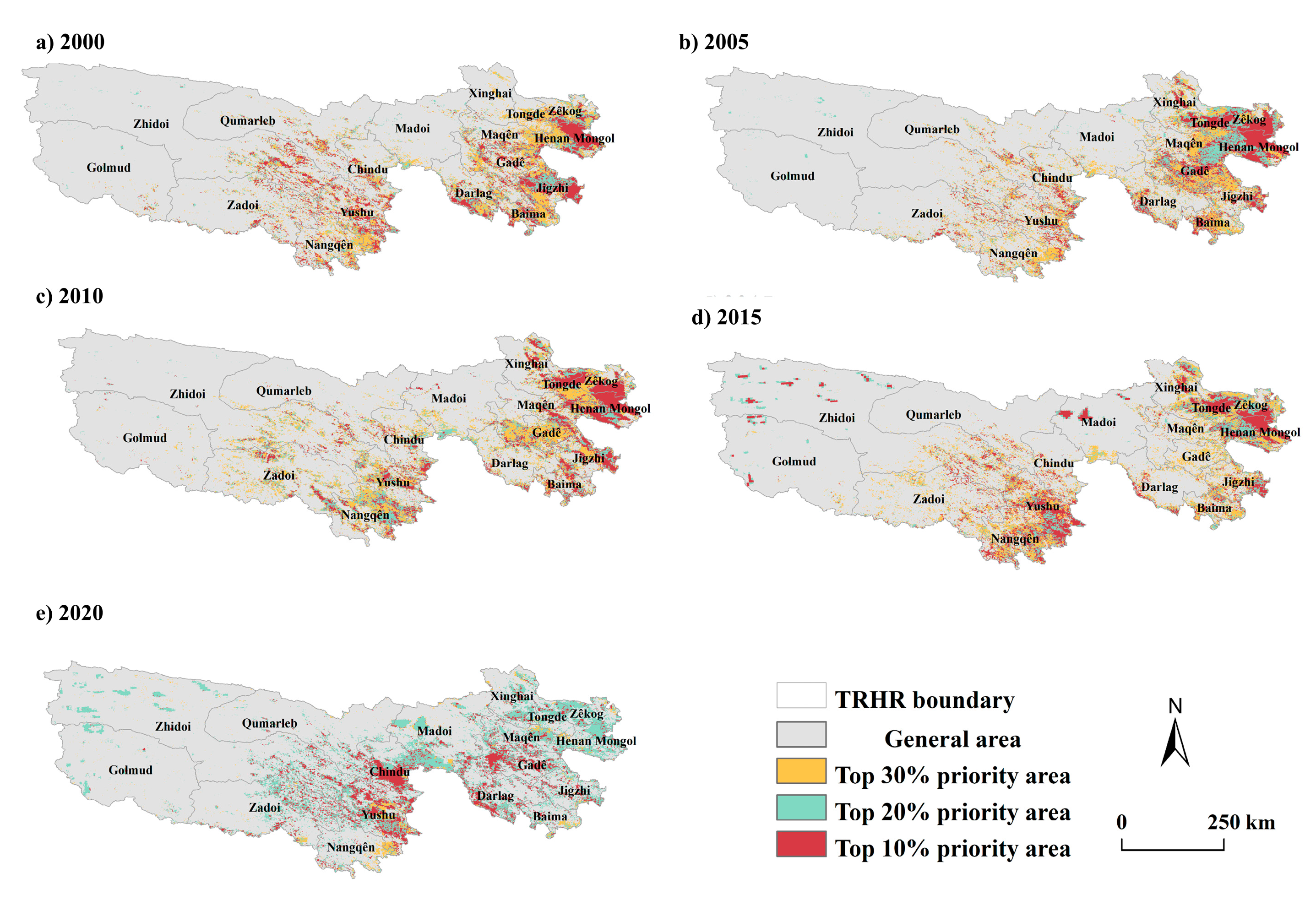
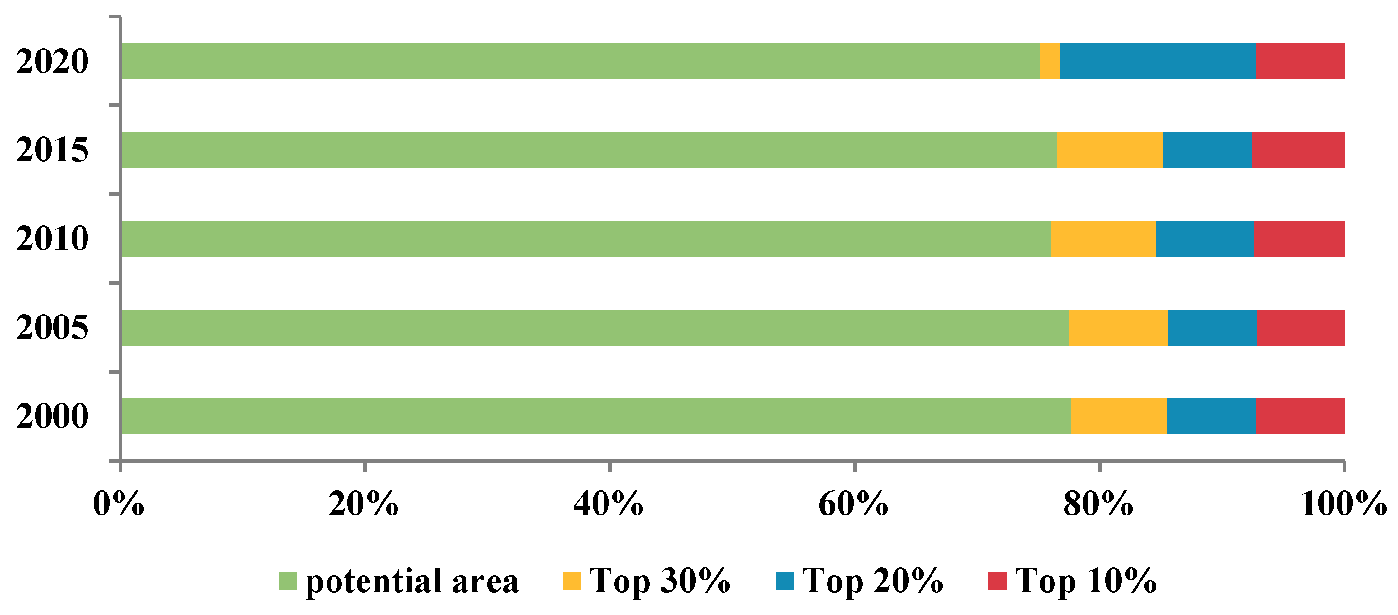
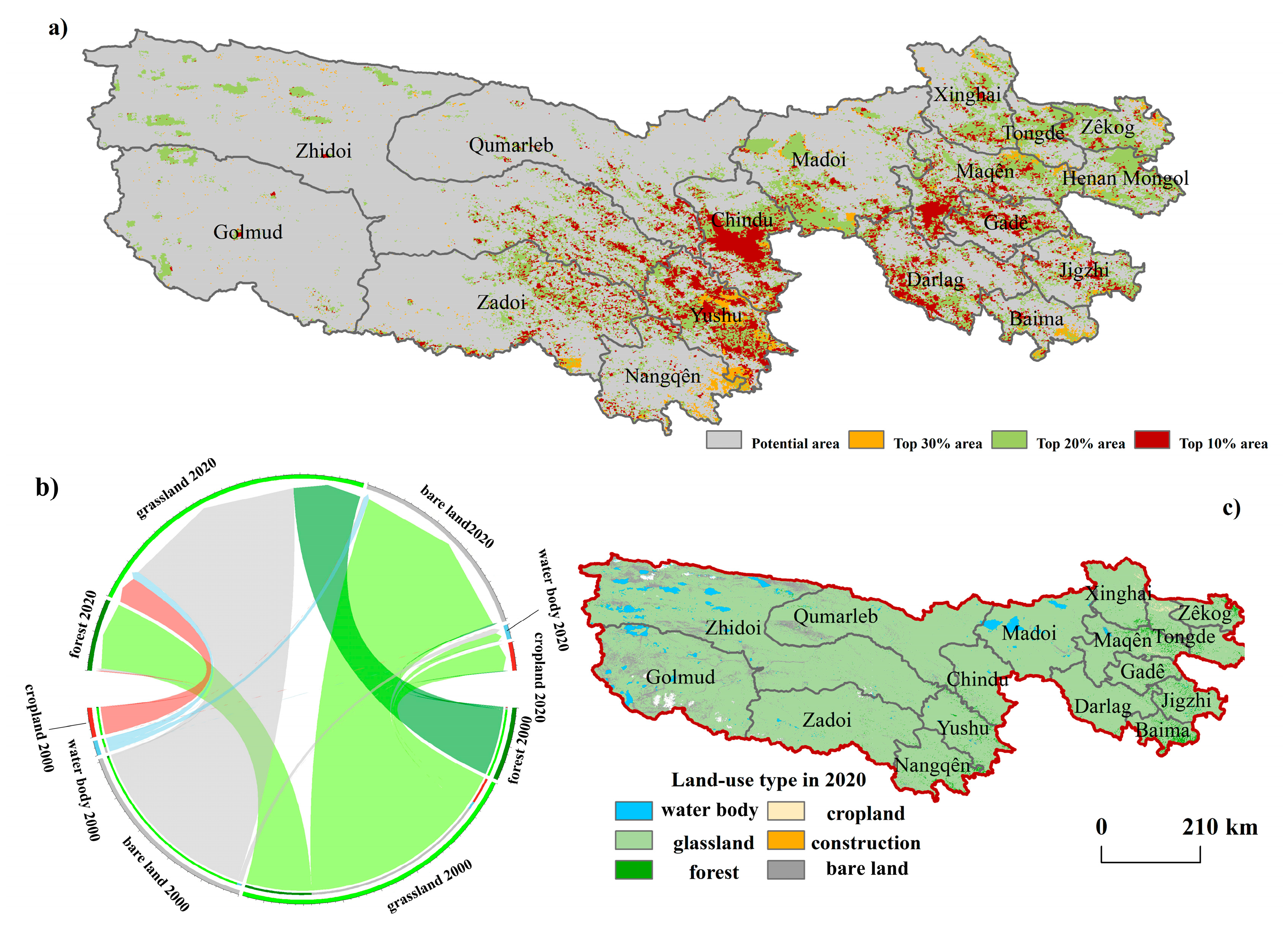
| Year | Potential Area (km2) | Top 30% Area (km2) | Top 20% Area (km2) | Top 10% Area (km2) |
|---|---|---|---|---|
| 2000 | 319,917 | 32,061 | 29,836 | 29,775 |
| 2005 | 318,850 | 33,349 | 30,081 | 29,288 |
| 2010 | 312,863 | 35,624 | 32,622 | 30,480 |
| 2015 | 315,171 | 35,437 | 30,018 | 30,963 |
| 2020 | 309,338 | 39,993 | 32,415 | 29,749 |
| Acronym | Full Name | Explanation | References |
|---|---|---|---|
| ES | ecological source | Ecological source areas represent continuum patches that are important for biodiversity, ecosystem services, and regional ecological security, or they have important radiative functions. | [1] |
| ESV | ecosystem service value | The direct and indirect benefits to human welfare offered by ecosystems. | [28] |
| RSEI | Remote Sensing Ecological Index | A composite ecological indicator that incorporates four key parameters—greenness, humidity, dryness, and heat—to evaluate the ecosystem quality. | [89] |
| MSPA | Morphological Spatial Pattern Analysis | An imaging method based on grid pixels of land use in the study area for calculation, identification, and segmentation | [10,90] |
| kNDVI | kernel Normalized Difference Vegetation Index | A vegetation index based on kernel methods expressed in terms of the spectral channels. | [40] |
| TRHR | Three-River Headwaters Region | The source of the Yangtze River, the Yellow River, and the Lantsang River. | [91] |
| GEE | Google Earth Engine | An image dataset processing cloud platform | [92] |
| CSI | Carbon Sink Index | A carbon sink revision index | - |
| LAI | Landscape Aesthetics Index | A landscape aesthetics revision index that consists of naturalness, the Shannon–Wiener diversity index, and the Euclidean distance to places of interest. | [63] |
| NEP | Net Ecosystem Productivity | The difference between net primary productivity (NPP) and soil heterotrophic respiration (Rh). | [93] |
| VFC | Vegetation Fraction Coverage | One of the most important indicators for measuring surface vegetation cover. | [94] |
| CAZ | Core-area zonation | A spatial priority rule that tries to retain core areas of all species. | [69] |
| ABF | Addictive–Benefit Function | A spatial priority rule that tries to retain core areas of all species. | [69] |
| NRs | Nature reserves | Pillars of biodiversity conservation. | [34] |
Disclaimer/Publisher’s Note: The statements, opinions and data contained in all publications are solely those of the individual author(s) and contributor(s) and not of MDPI and/or the editor(s). MDPI and/or the editor(s) disclaim responsibility for any injury to people or property resulting from any ideas, methods, instructions or products referred to in the content. |
© 2024 by the authors. Licensee MDPI, Basel, Switzerland. This article is an open access article distributed under the terms and conditions of the Creative Commons Attribution (CC BY) license (https://creativecommons.org/licenses/by/4.0/).
Share and Cite
Feng, X.; Huang, H.; Wang, Y.; Tian, Y.; Li, L. Identification of Ecological Sources Using Ecosystem Service Value and Vegetation Productivity Indicators: A Case Study of the Three-River Headwaters Region, Qinghai–Tibetan Plateau, China. Remote Sens. 2024, 16, 1258. https://doi.org/10.3390/rs16071258
Feng X, Huang H, Wang Y, Tian Y, Li L. Identification of Ecological Sources Using Ecosystem Service Value and Vegetation Productivity Indicators: A Case Study of the Three-River Headwaters Region, Qinghai–Tibetan Plateau, China. Remote Sensing. 2024; 16(7):1258. https://doi.org/10.3390/rs16071258
Chicago/Turabian StyleFeng, Xinyi, Huiping Huang, Yingqi Wang, Yichen Tian, and Liping Li. 2024. "Identification of Ecological Sources Using Ecosystem Service Value and Vegetation Productivity Indicators: A Case Study of the Three-River Headwaters Region, Qinghai–Tibetan Plateau, China" Remote Sensing 16, no. 7: 1258. https://doi.org/10.3390/rs16071258
APA StyleFeng, X., Huang, H., Wang, Y., Tian, Y., & Li, L. (2024). Identification of Ecological Sources Using Ecosystem Service Value and Vegetation Productivity Indicators: A Case Study of the Three-River Headwaters Region, Qinghai–Tibetan Plateau, China. Remote Sensing, 16(7), 1258. https://doi.org/10.3390/rs16071258