Article

Fusion of Hyperspectral and Multispectral Images with Radiance Extreme Area Compensation

1
Xi’an Institute of Optics and Precision Mechanics, Chinese Academy of Sciences, Xi’an 710119, China
2
Institute of Image Processing and Pattern Recognition, School of Information and Communications Engineering, Xi’an Jiaotong University, Xi’an 710049, China
3
University of Chinese Academy of Sciences, Beijing 100049, China
4
State Key Laboratory of Satellite Ocean Environment Dynamics, Second Institute of Oceanography, Ministry of Natural Resources, Hangzhou 310012, China
5
State Key Laboratory of Tropical Oceanography, South China Sea Institute of Oceanology, Chinese Academy of Sciences, Guangzhou 510301, China
*
Author to whom correspondence should be addressed.
Remote Sens. 2024, 16(7), 1248; https://doi.org/10.3390/rs16071248
Submission received: 22 February 2024 / Revised: 28 March 2024 / Accepted: 29 March 2024 / Published: 31 March 2024

Abstract

:
Although the fusion of multispectral (MS) and hyperspectral (HS) images in remote sensing has become relatively mature, and different types of fusion methods have their own characteristics in terms of fusion effect, data dependency, and computational efficiency, few studies have focused on the impact of radiance extreme areas, which widely exist in real remotely sensed scenes. To this end, this paper proposed a novel method called radiance extreme area compensation fusion (RECF). Based on the architecture of spectral unmixing fusion, our method uses the reconstruction of error map to construct local smoothing constraints during unmixing and utilizes the nearest-neighbor multispectral data to achieve optimal replacement compensation, thereby eliminating the impact of overexposed and underexposed areas in hyperspectral data on the fusion effect. We compared the RECF method with 11 previous published methods on three sets of airborne hyperspectral datasets and HJ2 satellite hyperspectral data and quantitatively evaluated them using 5 metrics, including PSNR and SAM. On the test dataset with extreme radiance interference, the proposed RECF method achieved well in the overall evaluation results; for instance, the PSNR metric reached 47.6076 and SAM reached 0.5964 on the Xiong’an dataset. In addition, the result shows that our method also achieved better visual effects on both simulation and real datasets.

1. Introduction

Hyperspectral (HS) remote sensing can obtain rich spectral information of ground objects and have broad application prospects in the fields of object detection [1], fine classification [2], and character attribute inversion [3]. However, due to limitations inherent in its imaging mechanism, hyperspectral remote sensing does not achieve the same level of spatial resolution as multispectral remote sensing, resulting in the loss of spatial texture information. The most common solution is to fuse hyperspectral data with multispectral (MS) data of a higher spatial resolution [4]. In recent years, hyperspectral remote sensing has developed rapidly, bringing a large number of hyperspectral remote sensing data sources and operationalization requirements for massive hyperspectral data fusion tasks [5]. Recently, Italy launched the PRecursore IperSpettrale della Missione Applicativa (PRISMA) earth observation satellite in March 2019 [6]; Germany launched the Environmental Mapping and Analysis Program (EnMAP) hyperspectral satellite in April 2022 [7,8]; and China launched GF-5 [9], ZY-1 02D [10], and HJ-2 A/B [11] satellites from 2018 to 2020 which carry different types of optical remote sensing payloads, including a hyperspectral camera. Simultaneous observation data from multiple sources in single satellite mission bring benefits to hyperspectral data fusion tasks with high spatial resolution data, which avoid the effects of atmospheric radiation transmission and changes in ground objects over time.
The main methods for the fusion of HS and MS images (his and MSI) can be divided into three categories: pan-sharpening-based methods, machine learning-based methods, and deep learning-based methods. The pan-sharpening methods extend the fusion approach of panchromatic images and MS images to the fusion of hyperspectral and multispectral data. They mainly include component substitution (CS)-based methods [12] and multi-resolution analysis (MRA)-based methods [13]. CS-based methods decompose the spatial and spectral information of hyperspectral and multispectral data and then replace the low-resolution (LR) spatial information of HS data with that of MS data to fuse into high-resolution (HR) hyperspectral data, as exemplified by the methods used in [14,15]. MRA-based methods use multiscale decomposition to obtain MS spatial detail information, which is then fused into the corresponding spectral bands of HS to obtain enhanced hyperspectral resolution, as seen in the methods used in [16,17]. Pan-sharpening methods, while able to achieve good spatial information results, suffer from more severe spectral distortion.
The machine learning-based method approach is to construct a mathematical model for HS and MS data fusion-based on machine learning theory, which mainly includes methods based on Bayesian theory, matrix decomposition, and tensor representation. Bayesian theory methods uses prior knowledge to establish a posterior distribution, providing an intuitive explanation for the fusion process [18,19,20]. Wei et al. adopted a Bayesian model based on sparse coding and dictionary learning to address fusion problems by introducing a maximum a posteriori (MAP) estimator [21]. Bayesian fusion methods achieve regularization through the prior distributions added by fusing scene data, such as l2-Gaussian priors, total variation priors, sparse priors, and low-rank priors [22,23,24]. Matrix decomposition methods utilize the spectral unmixing theory to decompose HS and MS data into endmember matrices and abundance matrices. High-resolution hyperspectral fusion is achieved by recombining the endmember matrix of HS data with the abundance matrix of MS data [25,26,27,28,29]. Yokoya et al. used coupled non-negative matrix factorization (CNMF) to extract the endmember matrices and abundance matrices of HS and MS data for image fusion [25]. Nezhad et al. combined sparse representation with image unmixing theory to acquire information reorganization between images [30]. Tensor representation methods treats hyper-spectral data as tensors, which can better preserve the spatial–spectral structure of image data compared to matrix decomposition methods [31,32,33]. Dian et al. [31] proposed a non-local sparse tensor decomposition method for HS data super-resolution. This method decomposes HSIs into sparse core tensors and dictionary estimates, where the dictionary and core tensors can be learned from LR-HSI and HR-MSI. Zhang et al. [34] proposed a low-rank Tucker decomposition model combined with two graphs to fuse HSI and MSI. Li et al. [35] treated HR-HSI as a three-dimensional tensor and proposed to solve the fusion problem by estimating the core tensor and dictionary along three modes. The machine learning-based methods make full use of the prior factors of images, such as sparsity, low rank, and global similarity, and have good interpretability and theoretical basis. They are commonly used in engineering practice. However, their ability to describe nonlinear factors in the fusion process is poor, and the fusion effect of abnormal areas in the image also needs to be improved.
Due to their advantages in solving nonlinear problems, deep learning-based methods are widely used in remote sensing applications such as target recognition, terrain classification, and attribute inversion [36,37,38]. Increasingly, researchers have begun to utilize deep learning for HS data fusion studies. Palsson et al. [39] introduced a three-dimensional convolutional neural network (3D-CNN) fusion approach to compensate for the potential loss of spatial information when processing three-dimensional HS data in two dimensions. Yang et al. [40] proposed a two-branch convolutional neural network (Two-CNN) method to extract spectral information from HS images and spatial information from MS images, fusing the features through a fully connected layer. Zhou et al. [41] developed a CNN-based pyramid fusion model consisting of an encoder and a pyramid fusion subnet. Xue et al. [42] proposed a variational fusion network, where the degradation model and data priors are implicitly represented by deep learning networks and jointly learned from training data. Su et al. [43] proposed a novel unsupervised Generative Adversarial Network (GAN) to address the HSI and MSI fusion problem with arbitrary point spread function (PSF) and spectral response function (SRF). Although deep learning methods can achieve better fusion results, they require a large amount of training data and suffer from issues such as overfitting and limited generalization ability [44].
Although existing hyperspectral and multispectral fusion algorithms have accomplished a good performance on well-preprocessed publicly available HS datasets. We found that extreme radiance areas widely exist in real hyperspectral remote sensing data, resulting in severe distortion of spectral information, which will have a significant impact on fusion results, as shown in Figure 1. These abnormal regions can be classified into two categories: overexposed regions and underexposed regions (low radiance). Both are unavoidable due to the imaging principles of hyperspectral cameras. For the high quantification requirements, hyperspectral cameras usually adopt fixed-gain imaging. Even if the gain setting ensures that the brightness of most ground objects is within the dynamic range, there will still be a small number of targets with specular reflection and other overexposure due to factors such as the surface material of the ground objects and the observation angle, which is reflected in the hyperspectral image as spike noise in certain bands. For low-reflectance ground objects such as water bodies or shadowed areas, the detector receives low energy from the ground objects, leading to a decrease in the signal-to-noise ratio when the detector’s background noise remains unchanged. Despite the fact that the abnormal regions only occupy a small portion of the hyperspectral data in terms of area, they are often the focus of attention for hyperspectral applications such as target recognition, change detection, and anomaly detection.
To enhance the effectiveness of hyperspectral fusion in radiance extreme areas, this paper proposes a hyperspectral and multispectral fusion algorithm architecture called RECF, which is based on radiance extreme compensation. This idea is built upon the architecture of spectral unmixing fusion methods. Based on the global iterative unmixing of hyperspectral and multispectral data in existing methods, the approach proposes utilizing local information constraints to process underexposed areas and utilizing multispectral data for replacement compensation in overexposed areas. Firstly, the overexposed regions are extracted (based on distinct characteristics) for subsequent processing. The Piecewise Smooth Non-Negative Matrix Factorization (PSNMF) is adopted as the data unmixing method, which can effectively suppress noise in both spatial and spectral dimensions. Then, during the iterative unmixing process, the HS data are reconstructed using the endmember and abundance matrices. By comparing the original HS data, error maps based on Spectral Angle Mapper (SAM) and Root Mean Square Error (RMSE) are derived to extract regions with a low signal-to-noise ratio (SNR). The constraint term of PSNMF is updated for regions with low SNR and regions with low average spectral band energy. Finally, the hyperspectral endmembers and multispectral abundances are combined to form the fused high-resolution hyperspectral data. For overexposed regions, compensation is achieved by replacing the multispectral abundances with those from non-overexposed regions with similar SAM values. The main contributions of this paper are as follows:
(1)
The novel RECF method is the first to focus on the impact of radiance extreme regions on hyperspectral fusion and explicitly proposes a solution framework.
(2)
To address the underexposed areas, effective region extraction is achieved through the reconstruction error map. By utilizing piecewise constrained non-negative matrix factorization, the influence of spectral noise caused by underexposed areas on fusion is effectively suppressed.
(3)
For overexposed regions, optimal replacement compensation is calculated with the help of multispectral data.
(4)
RECF is an unsupervised method that can be applied to the fusion of HS and MS remote sensing data in real-world applications. Through experiments with simulated and real data, its fusion effect on overexposed and underexposed regions is significantly better compared to the current advanced methods.
The remainder of this paper is organized as follows. Section 2 describes the spectral unmixing fusion model, constrained non-negative matrix factorization and the impact of targets in extreme brightness regions on fusion. Section 3 formulates the proposed fusion algorithm and optimization strategy. Section 4 elaborates the experimental results from both simulated and real data and provides an analysis of these results. Finally, the conclusion is given in Section 5.

2. Materials and Methods

2.1. Unmixing-Based Fusion Model

The hyperspectral and multispectral fusion task can be regarded as the recovery and reconstruction of high-spectral-resolution hyperspectral data (HH ∈ ℝLh×Nm) from low-spatial-resolution hyperspectral remote sensing observation data (HS ∈ ℝLh×Nh) and low-spectral-resolution multispectral remote sensing observation data (MS ∈ ℝLm×Nm). Lh and Lm represent the number of HS and MS bands, and Nh and Nm represent the number of pixels of the whole HS and MS data. The relationship between the observed HS and HH can be expressed as Equation (1), where S is the point spread function (PSF), and nh represents the noise and model error, including Truncation noise from overexposure and spectral noise from low response. The relationship between the observed MS and HH can be expressed as Equation (2), where R is the spectral response function (SRF), and nm represents the noise and model error. In practical applications, S is obtained through the registration estimation of the two types of data to be fused or approximated using an interpolation model, while R is derived from the radiometric calibration of the two types of data or estimated approximately, such as the method adopted in [45].
H S = H H S + n h
M S = R H H + n m
According to the Linear Mixing Model (LMM), each pixel in an HS image is composed of a linear combination of spectra from several endmembers [46]. For an HS image, all the endmember spectra constitute its endmember matrix, E = (E1, E2, ..., EK)L × K, where L is the number of spectral bands, and K is the number of endmembers. The linear combination coefficients of all pixels form the abundance matrix, A = (A1, A2, ..., AN)K × N, where K corresponds to the number of endmembers in the endmember matrix, and N is the total number of pixels. Therefore, the original hyperspectral data HS can be approximately represented as the product of its endmember matrix, Eh, and abundance matrix, Ah. Similarly, the original multispectral data MS can be approximately represented as the product of its endmember matrix, Em, and abundance matrix, Am. The fused high-resolution hyperspectral data can be approximately represented as the product of Eh and Am, as shown in Equation (3). Combining Equations (1) and (2), Ah can be seen as the convolution of Am with S, and Em can be seen as the convolution of Eh with R, as shown in Equations (4) and (5).
H H E h A m
H S H H S = E h A m S = E h A h
M S R H H = R E h A m = E m A m
Non-negative matrix factorization (NMF) is a commonly used spectral unmixing algorithm, characterized by the fact that all matrix elements after decomposition are non-negative [47,48]. The objective of fusing HS and MS data based on NMF is to minimize the expression shown in Equation (6), where Eh and Am are the targets that need to be iteratively optimized, and ‖·‖F represents the Frobenius norm. In addition to constraining Eh and Am to be non-negative, it is usually required that the sum of the column vectors in the abundance matrix, Am, is 1.
arg min E h , A m 1 2 E h A h H S F 2 + E m A m M S F 2 , s . t .   E h 0 , A m 0 , 1 K T A m = 1 N T

2.2. Piecewise Smoothness Constrained Non-Negative Matrix Factorization

Due to the inherent non-convexity of the NMF algorithm, there exist infinitely many solutions for non-negative matrix factorization, and it is not easy to converge to the global optimum. Therefore, apart from the non-negativity and sum-to-one constraints, other constraints on the endmember matrix and abundance matrix are also widely used. Among them, Piecewise Smoothness Constrained Non-Negative Matrix Factorization (PSNMF) incorporates piecewise smoothness constraints into NMF [49]. Smoothness is an inherent property of natural objects, describing their continuity and homogeneity in spatial and spectral dimensions. Therefore, smoothness is a commonly used constraint in spectral unmixing. Piecewise smoothness, as opposed to overall smoothness, allows for abrupt changes in certain areas, providing an advantage in preserving the spatial texture and spectral features of objects. This algorithm imposes smoothness constraints on both the endmember and abundance matrices, with the objective function as Equation (7).
arg min E , A 1 2 E A H S F 2 + α E g E E N + α A g A A N
where EN and AN represent the local neighborhoods of the endmember matrix, E, and abundance matrix, A, respectively; and αE and αA are the corresponding regularization coefficients. The function g() is a smoothing function both acting on E and A that adopts a discontinuous adaptive Markov Random Field model [49], as shown in Equations (8) and (9). Ei is an endmember spectrum in E, and Ni = (I − 1, i + 1) is its fixed wavelength range neighborhood. Apk represents the abundance located at position (p, k) in A, and Nijp = ((I − 1)j, (i + 1)j, i(j − 1), i(j + 1))) is its neighborhood. The positive parameter γ determines the shape of the function g(), and the γ for the spectral correlation (denoted as γE) and spatial correlation (denoted as γA) should have different values.
g E i E N i = i N i g E i E i = i N i e ( E i E i ) 2 / γ E + 1
g A p k A N p k = i j N i j p g A _ i j p A _ i j p = i j N i j p e ( A _ i j p A _ i j p ) 2 / γ A + 1

2.3. The Impact of Radiance Extreme Areas on Fusion

During the real-world process of hyperspectral remote sensing imaging via satellites, due to factors such as the performance of the hyperspectral camera itself, observation angles, atmospheric radiation transmission, and the reflection characteristics of ground objects, the acquired hyperspectral remote sensing data often suffer from quality degradation. In hyperspectral remote sensing images, this manifests as the presence of overexposed or underexposed regional targets, as shown in Figure 1.
The overexposed regions in hyperspectral remote sensing images are usually caused by specular reflections from highly reflective ground objects or due to special observation angles. Because of the need for quantitative remote sensing, hyperspectral remote sensing cameras typically use a fixed gain during imaging, and it is difficult to ensure that, within a wide spectral range, ground objects do not experience overexposure in any spectral band. In contrast, multispectral remote sensing has fewer spectral bands and more flexible gain settings, so overexposure is less common. The overexposed regions in hyperspectral remote sensing images have obvious characteristics: the full spectrum or partial spectral bands reach the maximum or zero value of the DN (Digital Number) quantization, leading to distortion of the hyperspectral curve.
The overly dark regions in hyperspectral remote sensing images are usually caused by low-reflectance ground objects, objects located in shadowed areas, or low solar altitude angles during imaging. Due to the low incident energy on the regional target, and the fact that hyperspectral cameras distribute this energy across various spectral bands, the effective signal energy for a single spectral band of the regional target is low. In contrast, multispectral remote sensing has fewer spectral bands but a wider spectral range for each band, so the same regional target has higher effective signal energy. The overly dark regions in hyperspectral remote sensing images manifest as increased noise, leading to false peak and valley features in the spectral curve of the regional target. Both overexposed and overly dark regions, if not specifically addressed during hyperspectral fusion, can degrade the fusion effect in those areas, particularly affecting the fusion of small targets.

3. Proposed Method

3.1. Idea of RECF

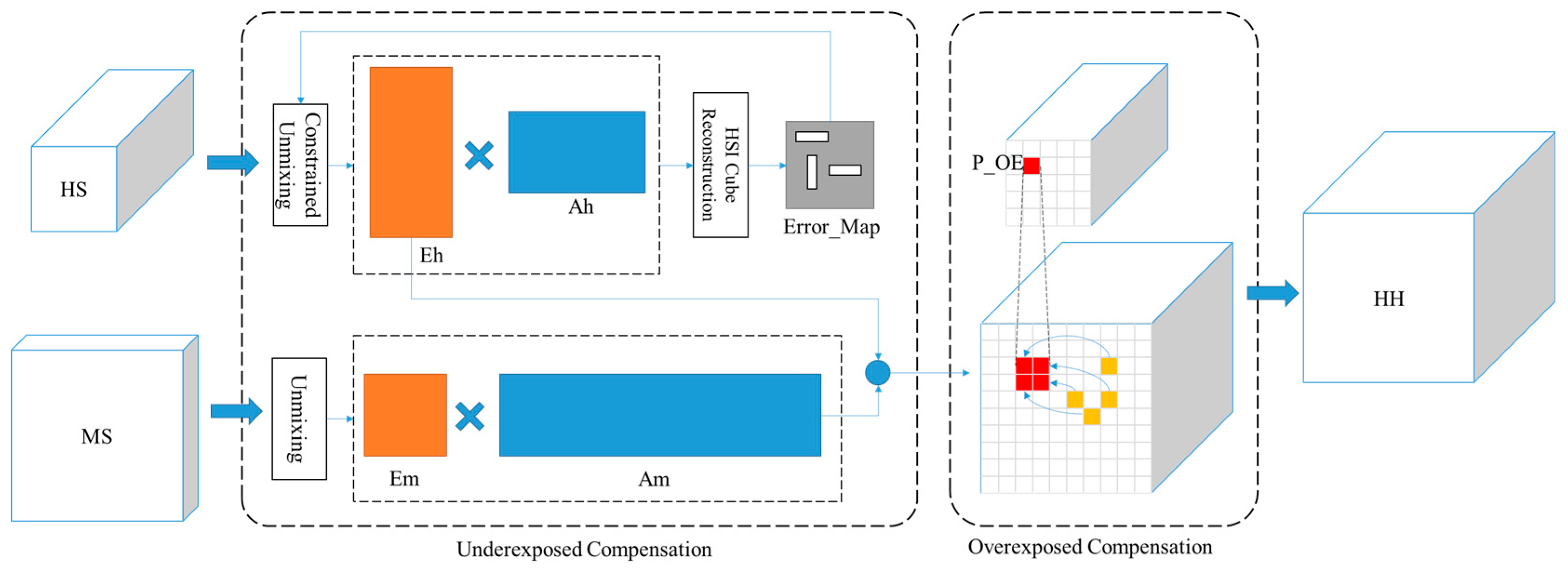
For the fusion of HS and MS data in real remote sensing scenarios, effectively dealing with extreme radiance areas of overexposure and underexposure is a practical problem to be solved. Based on the above motivation, we propose the RECF hyperspectral fusion algorithm with extreme radiance compensation, as shown in Figure 2. Eh and Ah represent the endmember and abundance matrices of HS data, Em and Am represent the endmember and abundance matrices of MS data, P_OE represents the overexposed pixels in hyperspectral data, and HH is the fused high-spatial-resolution hyperspectral data.
Based on the traditional unmixing-based HS/MS fusion architecture, RECF innovatively adds three processing steps specifically for extreme radiance areas.
Firstly, during the iterative unmixing process of hyperspectral data, a reconstruction error map characterizing the effect of spectral fusion is calculated. Typically, regions with low-hyperspectral signal-to-noise ratios have larger reconstruction errors, allowing for the extraction of overly dark regions during the iterative unmixing process through the error map.
Secondly, we use non-negative matrix factorization with local smoothing constraints for the iterative unmixing of HS data. The local smoothing constraints are applied separately to the hyperspectral endmember matrix and the hyperspectral abundance matrix. The local neighborhood range for the endmember matrix is determined using the energy distribution of each spectral band in the HS data, while the local neighborhood range for the abundance matrix is determined using the mask from the error map.
Lastly, for overexposed regions in the HS image, their spectral information is already distorted and cannot be used for fusion, requiring separate processing. After iterative unmixing and fusion in non-overexposed regions, optimal replacement compensation for the fused data in the overexposed regions is achieved using MS data.

3.2. Error Map

The error map represents the difference between the reconstructed HS data and the original HS data during the iterative unmixing process, specifically involving the endmember matrix and abundance matrix. In this paper, a combined configuration error map is constructed using the Spectral Angle Mapper (SAM) and Root Mean Square Error (RMSE), as shown in Equation (10). HSorg represents the original HS data, while Eh and Ah are the HS endmember matrix and HS abundance matrix obtained through iterative unmixing, respectively.
E r r o r M a p = ρ SAM ( H S o r g , E h A h ) + ( 1 ρ ) RMSE ( H S o r g , E h A h )
As shown in Figure 3, the SAM error characterizes differences in spectral curve features. Typically, regions with low signal-to-noise ratios or small target areas can lead to increased SAM errors in reconstructed HS data. The RMSE error characterizes differences in spectral energy intensity. Usually, regions with abnormal distributions of radiance energy intensity can cause an increase in RMSE errors (Figure 3). The construction of the error map should comprehensively consider both the SAM and RMSE. Based on the different focal objectives of fusion compensation, the weight parameters, ρ, can be empirically set. By binarizing the error map using methods such as Otsu’s method [50], regions with large reconstruction errors can be extracted through a binary mask, providing a local neighborhood range for subsequent smoothing constraints on the abundance matrix.

3.3. Local Smoothing Constraint for the Abundance Matrix

The smoothness of abundance originates from the spatial correlation of remote sensing ground objects. Adding a smoothness constraint to the abundance matrix during hyperspectral unmixing essentially utilizes the spatial correlation of adjacent ground objects to reduce the impact of HS data noise on fusion. The PSNMF [49] method uses a fixed template to calculate the abundance matrix local neighborhood, AN, in Section 2.2, which is represented as Nijp = ((I − 1)j, (i + 1)j, i(j − 1), i(j + 1))) in Equation (9). While fixed templates are computationally simple, they can introduce interference from different types of ground objects when processing the edges of similar ground objects, thereby reducing the spectral accuracy of the fused data at the edges.
Therefore, in this paper, the result of the convolving binary error map with a fixed template is used as the local neighborhood, Nijp, for the current position i, j of the abundance matrix, as shown in Figure 4. Here, the fixed template adopts a 3 × 3 pixel template, represented as Nijp = ((i − 1)(j − 1), (i − 1)j, (i − 1)(j + 1); i(j − 1), ij, i(j + 1); (i + 1)(j − 1), (i + 1)j, (i + 1)(j + 1)). By utilizing the error map to construct the local neighborhood of the abundance matrix, this approach achieves two main benefits. Firstly, it applies smoothing only to regions with large reconstruction errors, avoiding the impact of nearby ground objects on the original spectral features of other regions. Secondly, compared to a fixed local neighborhood template, this method enables fusion at the edges of similar ground objects to be free from the influence of different types of nearby ground objects.

3.4. Local Smoothing Constraint for the Endmember Matrix

The smoothness of endmember spectra originates from the correlation between spectral bands of ground objects. Adding a smoothness constraint to the endmember matrix during hyperspectral unmixing essentially utilizes the similarity between adjacent spectral bands in the spectral dimension to reduce the impact of hyperspectral data noise on fusion. The PSNMF [49] method also uses a fixed endmember matrix local neighborhood, EN, in Section 2.2, which is represented as Ni = (i − 1, i + 1) in Equation (8). While imposing a smoothing constraint on the endmember spectra can achieve noise suppression in the spectral dimension, it also weakens spectral features to some extent. Therefore, the local neighborhood range for smoothing should be carefully set.
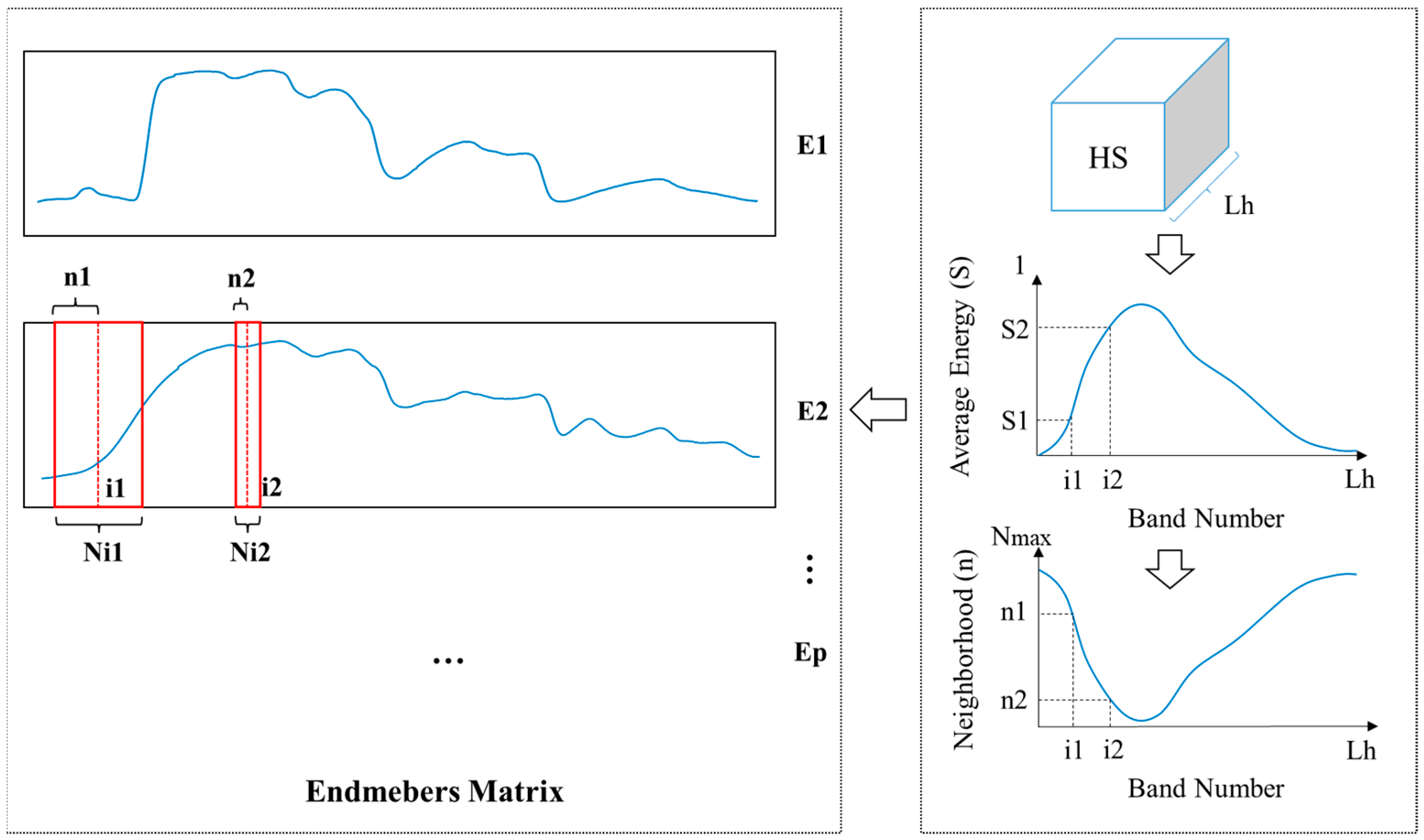
The HS data noise is proportional to signal energy, and the size of the local neighborhood range is inversely proportional to the average energy of each band in each endmember spectrum, i.e., Ni = (i − ni, i + ni). In this paper, a simple linear model is adopted, where ni = Nmax × (1 − Si), with Nmax being the maximum neighborhood range value, and Si being the normalized average energy of i-th band of HS data, as shown in Figure 5. This approach allows for a more dynamic and adaptive smoothing process that takes into account the varying noise levels and spectral characteristics of the hyperspectral data.

3.5. The Iterative Update Rule for PSNMF Fusion

We adopt the multiplicative update rules method used in [25] to iteratively update the HS and MS endmember and abundance matrices Eh, Ah, Em, and Am during the fusion process. For updating Eh and Ah, we use the iterative update rules of PSNMF [49], with the addition of a local smoothness constraint regularization term, as shown in Equations (11)–(14).
E h E h . H S A h T + α E E h . h E h E hN g E h E hN . /           E h A h A h T + α E E h . h E h E hN
A h A h . E h T H S + α A A h . h A h A hN g A h A hN . /           E h T E h A h + α A A h . h A h A hN
E m E m . M S A m T . / E m A m A m T
A m A m . E m T M S . / E m T E m A m

3.6. Compensation for Overexposed Areas

For the overexposed areas in the original HS data, prominent features of the overexposed data are extracted and excluded from the aforementioned unmixing and fusion process to prevent distorted spectral information from affecting the iterative optimization of the endmember and abundance matrices. After the unmixing and fusion steps, the hyperspectral endmember matrix, Eh, and the multispectral abundance matrix, Am, constitute the fused high-resolution hyperspectral data, HH. The location R_OE_MS corresponding to the overexposed area R_OE_HS of the original hyperspectral data is found in Am. Assuming that the multispectral data are not overexposed and that similar remote sensing objects also exist outside the overexposed area, the point (i′, j′) with the closest spectrum to the current overexposed area R_OE_MS pixel position (i, j) is searched for in the normally illuminated area R_MS. The spectral information at position (i, j) in the fused HH is then compensated for using the hyperspectral endmember matrix, Eh, and the abundance information of point (i′,j′), as shown in Equations (13) and (14). Here, ri,j represents the radiance intensity difference factor between objects (i, j) and (i′, j′), and it is calculated using Equation (17).
H H i , j = r i , j E h A m , i , j
arg min i , j SAM E m A m , i , j , E m A m , i , j i , j R _ M S _ O E i , j R _ M S
r i , j = i = 1 L m E m A m , i , j / i = 1 L m E m A m , i , j
Furthermore, the details of algorithm flowchart are described in Table 1. The value range of αE, αA, γE, γA, and ρ is from 0 to 1; they are selected as 0.5, 0.1, 0.01, 0.5, and 0.8 in this article, respectively.

4. Experiments

4.1. Experimental Data

To validate the effectiveness of the RECF method, we conducted controlled experiments using three airborne hyperspectral datasets from Pavia University, Chikusei, and Xiong’an, as well as hyperspectral and multispectral remote sensing images obtained from the HJ-2 satellite, as shown in Table 2.
(1)
Pavia University Datasets:
The Pavia University database contains a portion of hyperspectral data captured by the German airborne Reflective Optics System Imaging Spectrometer (ROSIS-03) over the city of Pavia, Italy, in 2003. The spectrometer continuously imaged 115 bands within the wavelength range of 0.43–0.86 μm, resulting in images with a spatial resolution of 1.3 m. The dataset measures 610 × 340 pixels and includes 9 classes of ground objects, such as trees, asphalt roads, bricks, and meadows, among others.
(2)
Chikusei Datasets:
The Chikusei database was captured by the Headwall Hyperspec-VNIR-C sensor in Chikusei, Japan, on 29 July 2014. This dataset contains 128 bands ranging from 343 to 1018 nanometers, with a size of 2517 × 2335 and a spatial resolution of 2.5 m. There are a total of 19 categories of ground objects, including urban and rural areas. This dataset was created and made publicly available by Dr. Naoto Yokoya and Prof. Akira Iwasaki from the University of Tokyo.
(3)
Xiong’an Datasets:
The Xiong’an dataset was collected by the full-spectrum multi-modal imaging spectrometer of the high-resolution aerial system developed by the Shanghai Institute of Technical Physics, Chinese Academy of Sciences. The spectral range covers 400–1000 nm with 250 bands, and the image size is 3750 × 1580 pixels. There are a total of 19 categories of ground objects, including rice stubble, grassland, elm, ash tree, etc.
(4)
HJ-2 satellite hyperspectral and multispectral data
The Environmental Disaster Reduction Satellites 2A and 2B are optical remote sensing satellites jointly developed and constructed by China’s Ministry of Ecology and Environment and Ministry of Emergency Management. They were launched on 27 September 2020 and have continuously produced remote sensing data products since then. They are equipped with four types of optical payloads: multispectral cameras, hyperspectral imagers, infrared cameras, and atmospheric correction instruments. Among them, the multispectral camera can collect multispectral data from five spectral bands, ranging from blue to near-infrared, with a spatial resolution of 16 m and a swath width of 800 km. The hyperspectral imager can collect visible HS data from 100 spectral bands with a spectral range of 450–900 nm, a spatial resolution of 48 m, and a swath width of 100 km. Since the collected HS and MS data are simultaneous and from the same perspective, there is no need to consider the impact of changes in the spectral and atmospheric lighting conditions of the ground objects due to time. At the same time, hyperspectral and multispectral data can also achieve high geometric registration accuracy.
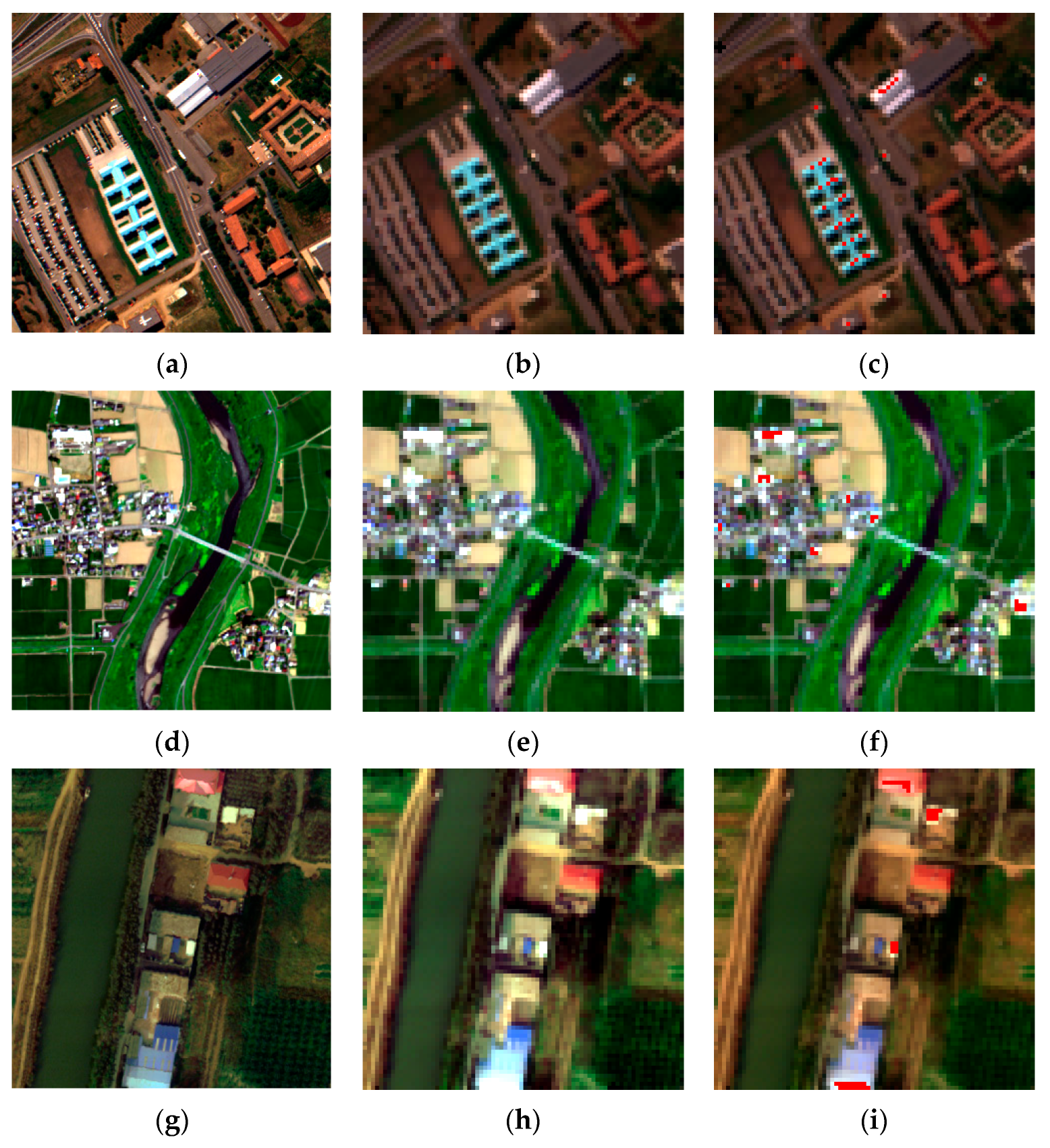
To compare the methods more intuitively and effectively, we performed uniform preprocessing operations on the airborne HS data. From each of the three HS datasets, we extracted a 320 × 320 pixel area with rich ground object types as the hyperspectral reference data. The hyperspectral reference data were downsampled by a factor of 4, using Gaussian filtering to simulate the HS data used in the fusion experiment, as shown in Figure 6b. The hyperspectral reference data were also convolved with the spectral response function of the multispectral data to simulate the MS data used in the fusion experiment, as shown in Figure 6a. Here, the spectral response function selected was that of the Sentinel-2 satellite’s multispectral blue, green, red, and near-infrared bands, so the simulated MS data had four bands. To verify the fusion effect of the algorithm on dark areas, Gaussian noise was added to the HS data to reduce its signal-to-noise ratio. To validate the fusion effect of the algorithm on overexposed data, overexposed pixels were manually added to the HS data based on the ground objects that were prone to overexposure, as indicated by the red markers in Figure 6c.
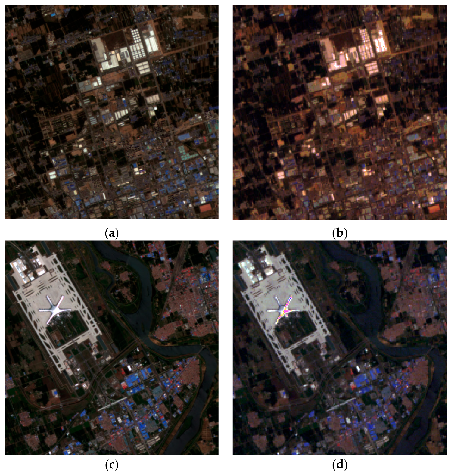
For the real in-orbit HS and MS remote sensing imagery of the HJ-2 satellite, we selected three different types of ground object scene data and performed the same preprocessing operations. Both HS and MS data used L1A-level remote sensing data products that had undergone relative radiometric correction and geometric rough correction. Due to the difference in spatial resolution between the two types of data, which is a factor of 3, the HS data were cropped to an experimental data size of 180 × 180 pixels, while the MS data were cropped to an experimental data size of 540 × 540 pixels. To verify the algorithm’s effectiveness in handling abnormal radiance areas, the selection of the experimental area included both overexposed and underexposed regions, as shown in Figure 7. Additionally, the measured spectral response functions of both HS and MS data were utilized as known parameters by the algorithm.

4.2. Compared Methods

In order to compare the performance of various methods for hyperspectral fusion under extreme radiance conditions, we selected the following methods as comparison algorithms: Gram–Schmidt algorithm (GS) [15], modulation transfer function generalized Laplacian pyramid (GLP) [17], smoothing filter-based intensity modulation (SFIM) [13], subspace-based regularization (HySure) [51], coupled non-negative matrix factorization (CNMF) [25], fast fusion of multi-band Images (FUSE) [52], coupled spectral unmixing (Lanaras) [27], coupled sparse tensor factorization (CSTF) [35], non-local sparse tensor factorization (NLSTF) [31], spatial and spectral fusion with CNN (SSFCNN) [53], and spatial–spectral reconstruction network (SSRNET) [54].
The comparison methods are all derived from the original author’s publicly available code, and the parameter values for each method were set according to the recommendations in the original papers or the default values in the public code. Methods GS, GLP, SFIM, HySure, CNMF, FUSE, and Lanaras are from HSMS Fusion Toolbox at https://openremotesensing.net/knowledgebase/hyperspectral-and-multi-spectral-data-fusion/hsmsfusiontoolbox/, accessed on 1 March 2023. Codes of CSTF and NLSTF are available at https://github.com/renweidian/CSTF, accessed on 1 March 2023 and https://github.com/renweidian/NLSTF, accessed on 1 March 2023. Codes of SSFCNN and SSRNET are available at https://github.com/hw2hwei/SSRNET, accessed on 1 March 2023.

4.3. Evaluation Metrics

To more comprehensively evaluate the effectiveness of different algorithms, we adopted five reference-based fusion quality evaluation metrics, namely PSNR, SAM, ERGAS, Q2n, and CC [4]. All of these evaluation metrics were used in the experiment on airborne hyperspectral data. For the fusion of satellite HJ-2 HS and MS remote sensing data, since there is no true high-resolution HS data as an evaluation reference, no-reference evaluation metrics are usually selected, such as QNR [12]. However, the no-reference evaluation metric is not applicable here because it uses the original HS data, which are interfered with by extreme radiance, as a reference in the spectral dimension. So, only the true-color composite images and spectral curves of fused data are presented which can already visually demonstrate the significant effectiveness of the method proposed in this paper. The definitions of each fusion evaluation metric are as follows:
(1)
PSNR
The peak signal-to-noise rate (PSNR) for each band of HSI is defined as
PSNR = 1 L h i = 1 L h 10   log 10 max H Re f i F 2 H Re f i H H i F 2
(2)
SAM
Spectral angle mapper (SAM) evaluates the spectral distortion and is defined as
SAM = 1 N m j = 1 N m arccos H H j T H Re f j H H j T 2 H Re f j 2
(3)
ERGAS
The relative global dimensional synthesis error (ERGAS) reflects the global quality of the fused results and is defined as follows (where d is spatial downsampling factor, and μk is the mean of HH):
ERGAS = 100 d 1 L h i = 1 L h H Re f i H H i F 2 μ k 2
(4)
Q2n
Q2n is a generalization of the universal image quality index (UIQI) and an extension of the Q4 index to HS images based on hypercomplex numbers.
Q 2 N × N n = σ z , v σ z σ v 2 z ¯ v ¯ z ¯ 2 + v ¯ 2 2 σ z σ v σ z 2 + σ v 2
(5)
CC
The correlation coefficient (CC) is computed as follows, where ρ is the Pearson correlation coefficient:
C C = 1 L h i = 1 L h ρ H Ref i , H H i

4.4. Experimental Results

(1)
Results on the airborne HS dataset
The evaluation metric results of various methods on the airborne HS dataset are shown in Table 3, Table 4 and Table 5. It can be seen that our RECF method has clear advantages in the three metrics of PSNR, ERGAS, and CC, and it also performs well in the two metrics of SAM and Q2n. In the Pavia University dataset, the RECF method achieved optimal values for PSNR, ERGAS, Q2n, and CC metrics, with scores of 44.6691, 1.4514, 0.9866, and 0.9949, respectively, while achieving a second-best value for the SAM metric, with a score of 2.2393. In the Chikusei dataset, the RECF method obtained optimal values for PSNR, ERGAS, and CC metrics with scores of 49.9857, 2.2541, and 0.9926, respectively, and once again, a second-best value for the SAM metric, with a score of 2.2393. The Xiong’an dataset simulated severe extreme radiance interference, where the RECF method demonstrated remarkable effectiveness, significantly outperforming other methods, with its PSNR, SAM, ERGAS, Q2n, and CC metrics achieving scores of 47.6076, 0.5964, 0.3739, 0.9844, and 0.9985, respectively.
In addition, among the other comparison algorithms, the GLP, NLSTF, and SSRNET methods also achieve good results. The GLP algorithm performs well in the SAM metric, NLSTF has a better effect in the PSNR metric, and the deep learning-based SSRNET method also achieves overall good results in the comprehensive metrics.
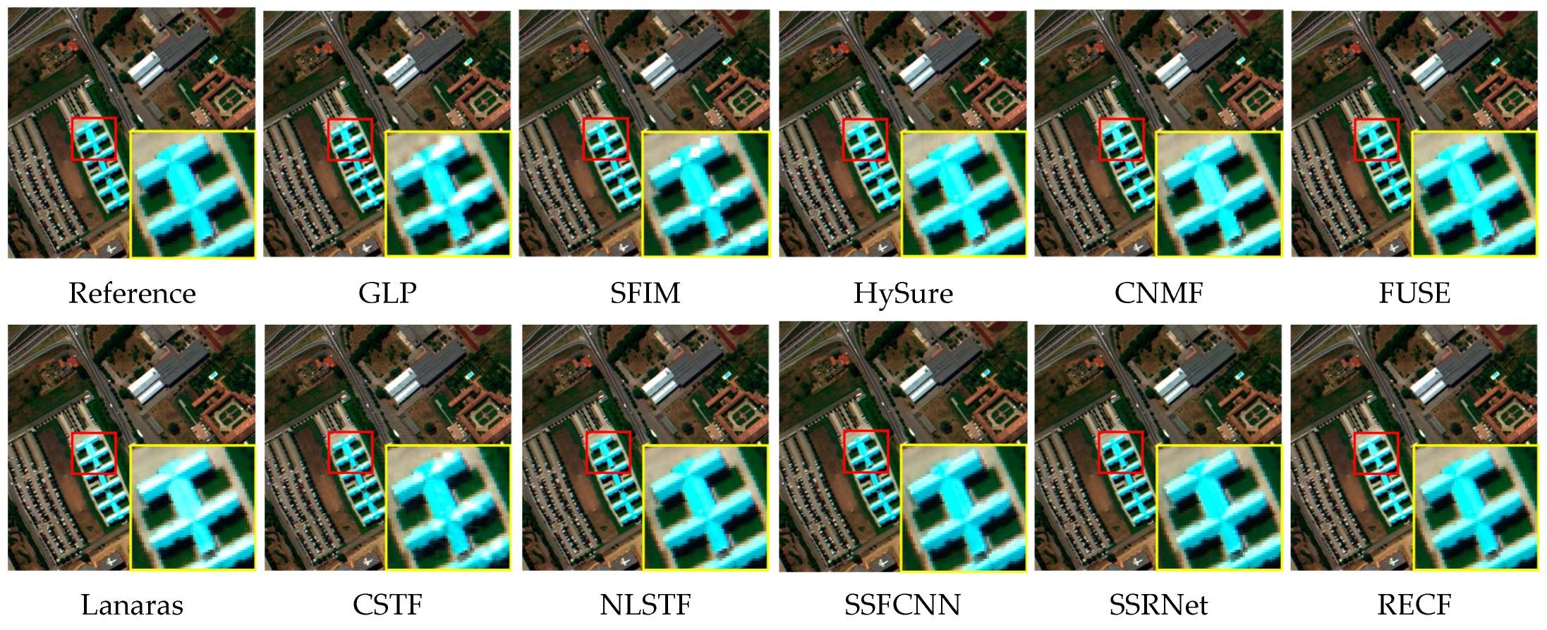
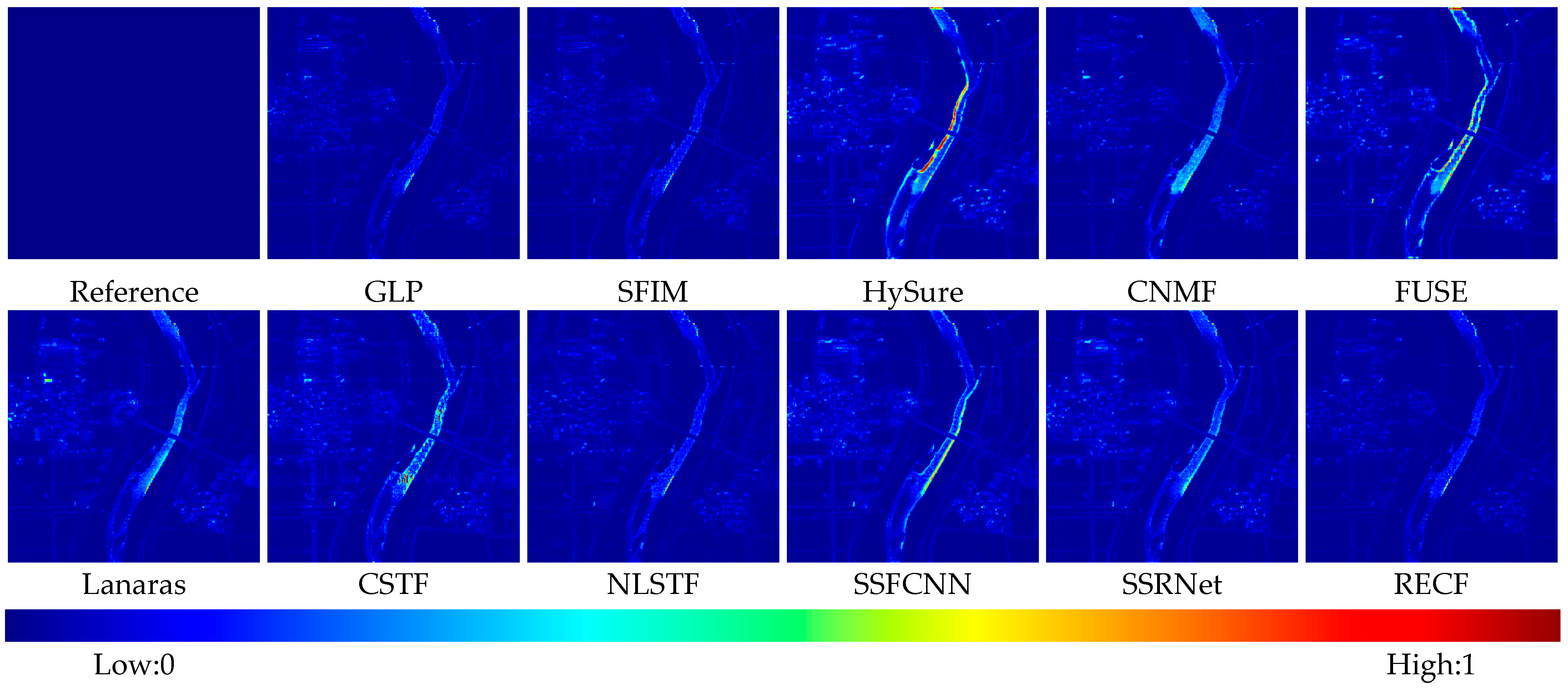
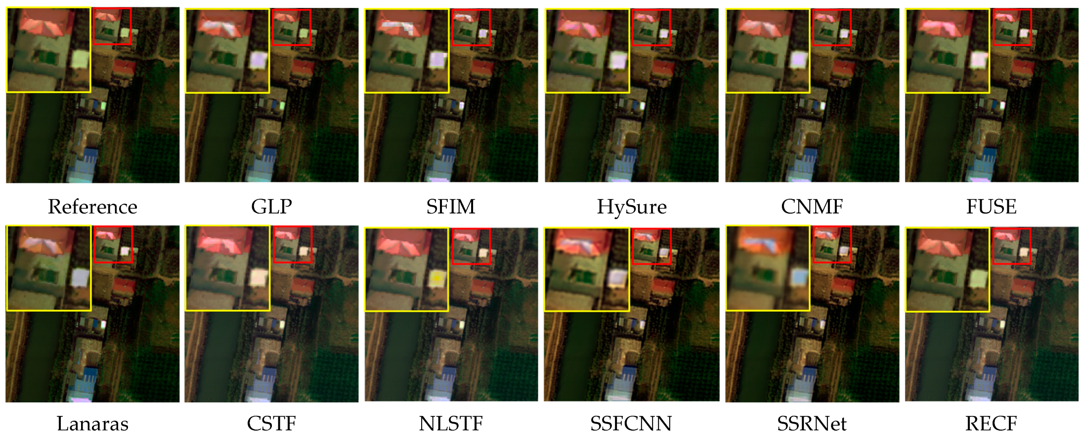
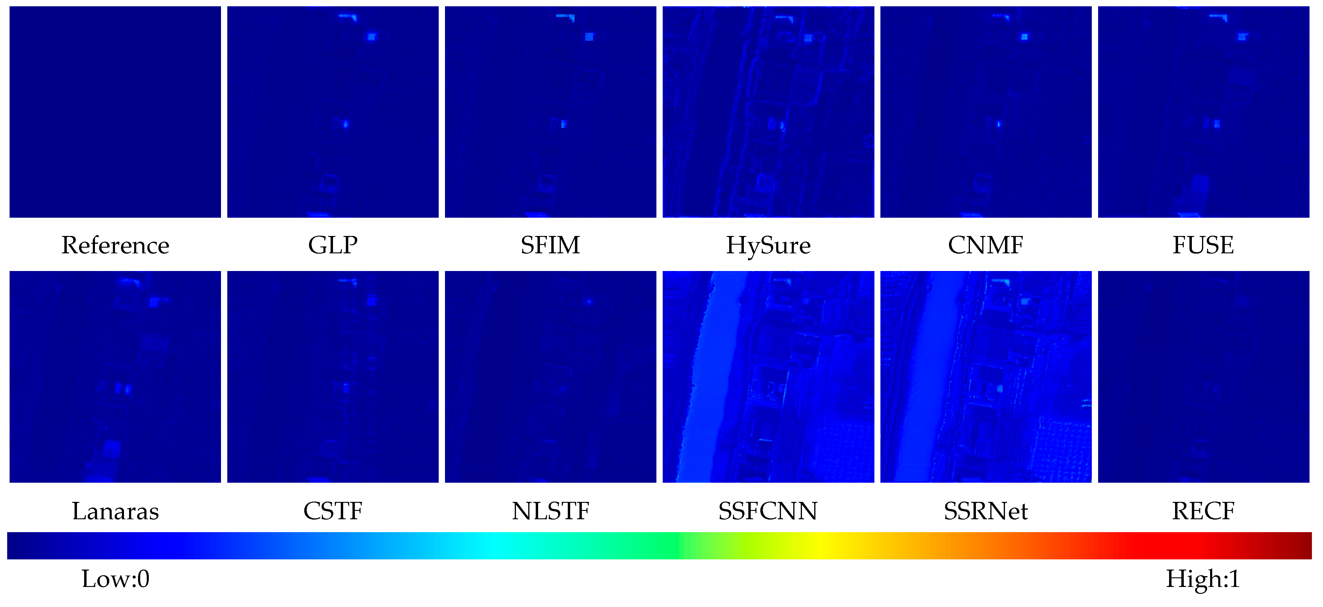
The performance of various methods on the true color band composite images and SAM-maps of the airborne HS dataset is shown in Figure 8, Figure 9, Figure 10, Figure 11, Figure 12 and Figure 13. Through the true color band composite images, it can be seen that our proposed RECF method achieves the most visually impressive results for overexposed areas. The overexposure phenomenon in the experimental HS data is effectively eliminated in the fused high-resolution hyperspectral data. In the true color images of the fusion results from the three datasets, this conclusion can be clearly seen through the locally enlarged overexposed buildings in the yellow box in Figure 8, Figure 10 and Figure 12. In addition, by comparing with the reference data, the color of the overexposed areas processed by the RECF algorithm is effectively preserved, indicating that the RECF method achieves good spectral fidelity.
Through the SAM-maps, it can be seen that, for low-radiance areas such as water bodies or shadows, our proposed RECF method also achieves the best visual results, with SAM errors remaining low in these areas. The conclusion can be clearly observed from the river areas in the SAM-maps of the fusion results from the Chikusei dataset (Figure 11) and the Xiong’an dataset (Figure 13). A higher SAM value represents a greater spectral error, while the RECF method maintains the lowest SAM values in the river areas.
Among other methods, NLSTF and SSRNet have achieved good visual effects on true color band composition images and SAM-maps.
Overall, on the airborne HS dataset with superimposed overexposure and underexposure treatments, the RECF algorithm achieves the most comprehensive and excellent metric results and stands out in terms of visual effects.
(2)
Results on HJ-2 satellite HS remote sensing images
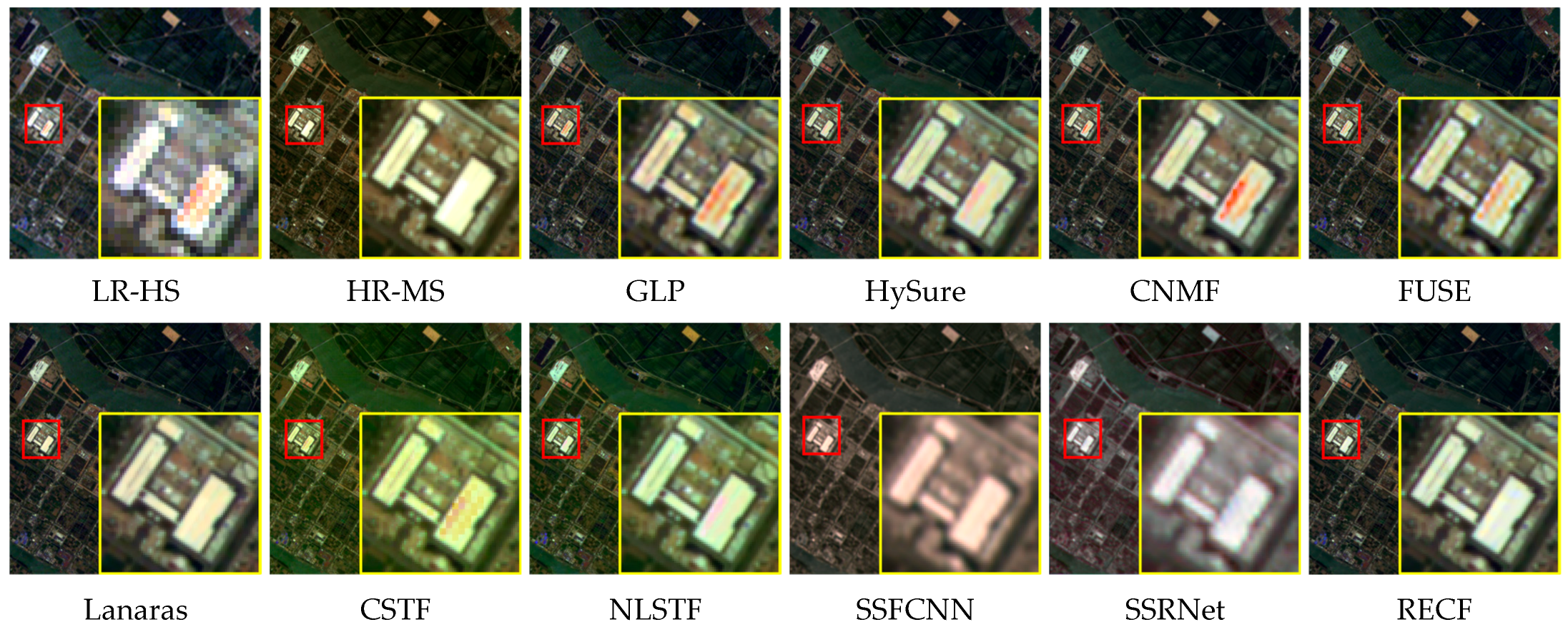
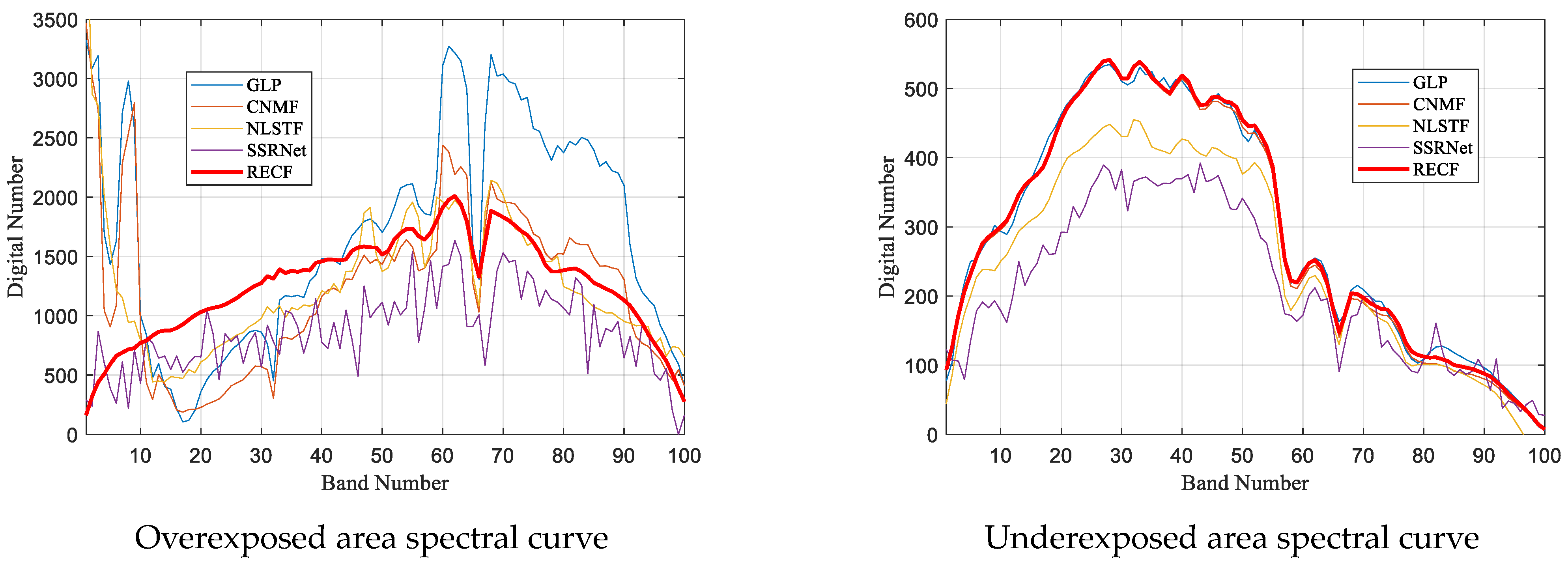
The performance of various methods on real on-orbit HS and MS remote sensing data from the HJ-2 satellite is shown in Figure 14, Figure 15 and Figure 16 and spectral curves of fused HH data are shown in Figure 17. Three typical scenes were selected for the experiment, including manmade buildings, airports, vegetation, water bodies, and other ground features. From the original LR-HS images, it can be observed that overexposure is a common issue in real HS remote sensing images. Furthermore, due to the imaging mechanism of the camera, the spectrum of overexposed areas may be chaotic, manifesting as color distortion in true-color images, such as the red color on the roof of the airport terminal in Scene 2 (Figure 15).
Due to the absence of reference data and the lack of no-reference evaluation metrics suitable for hyperspectral fusion affected by extreme radiance interference, a subjective evaluation was conducted here solely based on the visual effects of the true-color composite images of the fused data. It can be seen that the RECF algorithm proposed in this paper achieves better results on this metric. In the fused HR HS true color composite images, the RECF algorithm outperforms other algorithms, especially in overexposed areas where its impact is almost visually undetectable, and the fused data quality is close to that of the multispectral true color band composite images.
It should be noted that the deep learning method SSRNet, which we selected for processing real HS remote sensing data fusion tasks, exhibits significant distortion in both color information and texture details. This is because SSRNet is a supervised learning method, and we trained the model using the same experimental approach as for the airborne HS dataset by constructing training data through downsampling of HS data. However, the modal differences between actual MS and HS data differ from those between HS data and its own downsampled version, making this approach unsuitable for HS data fusion tasks in real-world applications.

4.5. Discussion

To validate the effectiveness of the proposed RECF method for hyperspectral fusion under extreme radiance conditions, including overexposed and underexposed areas, this paper conducted controlled experiments using airborne hyperspectral data and real on-orbit HS and MS remote sensing data from the HJ-2 satellite.
In the airborne HS data experiment, we selected and extracted specific a scene from the dataset that contains both high-radiance and low-radiance regions, artificially constructed overexposed pixels, and added noise to simulate the low-SNR characteristic of the underexposed areas. The degree of preprocessing we apply to the experimental scene data determines the evaluation metric results. By adding more overexposed areas and greater noise, the proposed method achieves more significant effects.
In the HJ-2 satellite HS/MS data experiment, we evaluate the proposed method only based on the visual effects of the fused images and spectral curves. We do not employ a reduced resolution of the original HS data for reference-based evaluation, nor do we use unsupervised fusion evaluation metrics. This is because both approaches consider the spectral information of the original HS data as ground truth reference, which does not align with the actual problem that the proposed method intends to solve.
We also observed that supervised learning and data-driven deep learning methods can suffer from significant distortion in fusion outcomes during practical tasks. This is due to the lack of HR HS data for supervised learning in real-world scenarios. Alternative approaches, such as training deep models through the downsampling of HS data, are limited in effectiveness due to differences in data modalities. Therefore, we believe that the focus of hyperspectral fusion research for practical applications should be on unsupervised learning methods.

5. Conclusions

This paper proposes a hyperspectral and multispectral data fusion algorithm called RECF (radiance extreme area compensation fusion) to address the severe spectral distortion issues. Based on the traditional unmixing-based fusion architecture, RECF adds the following steps, including constructing an error map during iterative unmixing, adding local smoothing constraints to the endmember and abundance matrices, and utilizing multispectral data for overexposure compensation.
Based on three airborne hyperspectral datasets from Pavia University, Chikusei, and Xiong’an, we simulated hyperspectral data affected by extreme radiance interference and conducted a reference-based evaluation. RECF achieved the best results in the overall evaluation; for instance, its PSNR reached 47.6076 and SAM reached 0.5964 on the Xiong’an dataset. Additionally, we conducted experiments on HJ-2 satellite hyperspectral and multispectral data. RECF also achieved optimal visual effects on both the fused images and spectral curves, thus demonstrating that our method is particularly well-suited for handling unsupervised fusion tasks of real hyperspectral and multispectral remote sensing data.
The fusion method-based on radiance extreme compensation essentially proposes the idea of utilizing the local similarity of remote sensing ground object spectra to achieve fusion compensation for underexposed areas, and leveraging the imaging mechanisms of multispectral data that are less prone to overexposure to achieve replacement compensation for overexposed areas after fusion. In this paper, we combined it with the spectral unmixing method of non-negative mean decomposition and achieved significant results. In the future, we can also explore combining it with other fusion methods, such as tensor decomposition and unsupervised deep learning.

Author Contributions

Y.W. wrote the manuscript; Y.W., J.C. (Jianyu Chen) and X.M. presented the main idea of this work; Y.W., T.C. and X.F. wrote the program code and completed all experiments; S.W., J.L. and G.Z. revised the paper structure; H.L. and Y.L. provided the simulated data; J.C. (Junyu Chen), X.M. and S.L. supervised the work and contributed to the experiments and discussions. All authors have read and agreed to the published version of the manuscript.

Funding

This study was supported by National Natural Science Foundation of China under Grant 42176182; the National Science Basic Research Foundation of Shaanxi Province under Grant 2023-YBGY-390; the State Key Laboratory of Tropical Oceanography, South China Sea Institute of Oceanology, Chinese Academy of Sciences (Project No. LTO2206); Public Fund of the State Key Laboratory of Satellite Ocean Environment Dynamics, Second Institute of Oceanography, Ministry of Natural Resources, under Grant QNHX3126; and the West Light Foundation of The Chinese Academy of Sciences 2023.

Data Availability Statement

Pavia University, Chikusei and Xiong’an datasets can be obtained from the following links: https://www.ehu.eus/ccwintco/index.php/Hyperspectral_Remote_Sensing_Scenes#Pavia_University_scene, accessed on 1 March 2023; https://naotoyokoya.com/Download.html, accessed on 1 March 2023 and http://www.hrs-cas.com/a/share/shujuchanpin/2019/0501/1049.html, accessed on 1 March 2023. HJ-2 HSI and MSI data of this study cannot be publicly accessed because the data owner has not allowed it.

Conflicts of Interest

The authors declare no conflict of interest.

References

  1. Lin, S.; Zhang, M.; Cheng, X.; Wang, L.; Xu, M.; Wang, H. Hyperspectral Anomaly Detection via Dual Dictionaries Construction Guided by Two-Stage Complementary Decision. Remote Sens. 2022, 14, 1784. [Google Scholar] [CrossRef]
  2. Liu, M.; Yu, T.; Gu, X.; Sun, Z.; Li, J. The Impact of Spatial Resolution on the Classification of Vegetation Types in Highly Fragmented Planting Areas Based on Unmanned Aerial Vehicle Hyperspectral Images. Remote Sens. 2020, 12, 146. [Google Scholar] [CrossRef]
  3. Bannari, A.; Staenz, K.; Champagne, C.; Khurshid, K.S. Spatial variability mapping of crop residue using hyperion (eo-1) hyperspectral data. Remote Sens. 2018, 7, 8107–8127. [Google Scholar] [CrossRef]
  4. Yokoya, N.; Grohnfeldt, C.; Chanussot, J. Hyperspectral and Multispectral Data Fusion: A comparative review of the recent literature. IEEE Geosci. Remote Sens. Mag. 2017, 5, 29–56. [Google Scholar] [CrossRef]
  5. Ren, K.; Sun, W.; Meng, X.; Yang, G.; Du, Q. Fusing China GF-5 Hyperspectral Data with GF-1, GF-2 and Sentinel-2A Multispectral Data: Which Methods Should Be Used? Remote Sens. 2020, 12, 882. [Google Scholar] [CrossRef]
  6. Pignatti, S.; Acito, N.; Amato, U.; Casa, R.; Castaldi, F.; Coluzzi, R.; De, B.R.; Diani, M.; Imbrenda, V.; Laneve, G. Environmental products overview of the Italian hyperspectral prisma mission: The SAP4PRISMA project. In Proceedings of the Geoscience & Remote Sensing Symposium, Milan, Italy, 26–31 July 2015. [Google Scholar]
  7. Stuffler, T.; Kaufmann, C.; Hofer, S.; FöRster, K.P.; Schreier, G.; Mueller, A.; Eckardt, A.; Bach, H.; Penné, B.; Benz, U. EnMAP Hyperspectral Imager: An advanced optical payload for future applications in Earth observation programs. Acta Astronaut. 2007, 61, 115–120. [Google Scholar] [CrossRef]
  8. Keller, S.; Braun, A.C.; Hinz, S.; Weinmann, M. Investigation of the impact of dimensionality reduction and feature selection on the classification of hyperspectral EnMAP data. In Proceedings of the 2016 8th Workshop on Hyperspectral Image and Signal Processing: Evolution in Remote Sensing (WHISPERS), Los Angeles, CA, USA, 21–24 August 2016. [Google Scholar]
  9. Ye, X.; Ren, H.; Liu, R.; Qin, Q.; Liu, Y.; Dong, J. Land Surface Temperature Estimate From Chinese Gaofen-5 Satellite Data Using Split-Window Algorithm. IEEE Trans. Geosci. Remote Sens. 2017, 55, 5877–5888. [Google Scholar] [CrossRef]
  10. Sun, W.; Liu, K.; Ren, G.; Liu, W.; Yang, G.; Meng, X.; Peng, J. A simple and effective spectral-spatial method for mapping large-scale coastal wetlands using China ZY1-02D satellite hyperspectral images. Int. J. Appl. Earth Obs. Geoinf. 2021, 104, 102572. [Google Scholar] [CrossRef]
  11. Chen, T.; Su, X.; Li, H.; Li, S.; Liu, J.; Zhang, G.; Feng, X.; Wang, S.; Liu, X.; Wang, Y.; et al. Learning a Fully Connected U-Net for Spectrum Reconstruction of Fourier Transform Imaging Spectrometers. Remote Sens. 2022, 14, 900. [Google Scholar] [CrossRef]
  12. Vivone, G.; Alparone, L.; Chanussot, J.; Mura, M.D.; Garzelli, A.; Licciardi, G.A.; Restaino, R.; Wald, L. A Critical Comparison Among Pansharpening Algorithms. IEEE Trans. Geoence Remote Sens. 2015, 53, 2565–2586. [Google Scholar] [CrossRef]
  13. Selva, M.; Aiazzi, B.; Butera, F.; Chiarantini, L.; Baronti, S. Hyper-Sharpening: A First Approach on SIM-GA Data. IEEE J. Sel. Top. Appl. Earth Obs. Remote Sens. 2015, 8, 3008–3024. [Google Scholar] [CrossRef]
  14. Chen, Z.; Pu, H.; Wang, B.; Jiang, G.M. Fusion of Hyperspectral and Multispectral Images: A Novel Framework Based on Generalization of Pan-Sharpening Methods. IEEE Geosci. Remote Sens. Lett. 2014, 11, 1418–1422. [Google Scholar] [CrossRef]
  15. Aiazzi, B.; Baronti, S.; Selva, M. Improving Component Substitution Pansharpening through Multivariate Regression of MS+Pan Data. IEEE Trans. Geosci. Remote Sens. 2007, 45, 3230–3239. [Google Scholar] [CrossRef]
  16. Gomez, R.B.; Jazaeri, A.; Kafatos, M. Wavelet-based hyperspectral and multispectral image fusion. Proc. SPIE—Int. Soc. Opt. Eng. 2001, 4383, 36–42. [Google Scholar]
  17. Aiazzi, B.; Alparone, L.; Baronti, S.; Garzelli, A.; Selva, M. MTF-Tailored Multiscale Fusion of High-Resolution MS and Pan Imagery. Photogramm. Eng. Remote Sens. 2015, 72, 591–596. [Google Scholar] [CrossRef]
  18. Wei, Q.; Bioucas-Dias, J.; Dobigeon, N.; Tourneret, J.Y. Hyperspectral and Multispectral Image Fusion based on a Sparse Representation. IEEE Trans. Geosci. Remote Sens. 2015, 53, 3658–3668. [Google Scholar] [CrossRef]
  19. Akhtar, N.; Shafait, F.; Mian, A. Bayesian sparse representation for hyperspectral image super resolution. In Proceedings of the IEEE Conference on Computer Vision & Pattern Recognition, Boston, MA, USA, 7–12 June 2015. [Google Scholar]
  20. Wei, Q.; Dobigeon, N.; Tourneret, J.Y. Bayesian Fusion of Multi-Band Images. IEEE J. Sel. Top. Signal Process. 2015, 9, 1117–1127. [Google Scholar] [CrossRef]
  21. Hardie, R.C.; Eismann, M.T.; Wilson, G.L. MAP Estimation for Hyperspectral Image Resolution Enhancement Using an Auxiliary Sensor. IEEE Trans. Image Process. 2004, 13, 1174–1184. [Google Scholar] [CrossRef] [PubMed]
  22. Bresson, X.; Chan, T.F.; Chan, T.F.C. Fast dual minimization of the vectorial total variation norm and applications to color image processing. Inverse Probl. Imaging 2017, 2, 455–484. [Google Scholar] [CrossRef]
  23. Rong, K.; Jiao, L.; Wang, S.; Liu, F. Pansharpening Based on Low-Rank and Sparse Decomposition. IEEE J. Sel. Top. Appl. Earth Obs. Remote Sens. 2017, 7, 4793–4805. [Google Scholar] [CrossRef]
  24. Zhang, K.; Wang, M.; Yang, S. Multispectral and Hyperspectral Image Fusion Based on Group Spectral Embedding and Low-Rank Factorization. IEEE Trans. Geosci. Remote Sens. 2017, 55, 1363–1371. [Google Scholar] [CrossRef]
  25. Yokoya, N.; Yairi, T.; Iwasaki, A. Coupled Nonnegative Matrix Factorization Unmixing for Hyperspectral and Multispectral Data Fusion. IEEE Trans. Geosci. Remote Sens. 2012, 50, 528–537. [Google Scholar] [CrossRef]
  26. Akhtar, N.; Shafait, F.; Mian, A. Sparse Spatio-Spectral Representation for Hyperspectral Image Super-Resolution. In Proceedings of the European conference on computer vision, Zurich, Switzerland, 6–12 September 2014. [Google Scholar]
  27. Lanaras, C.; Baltsavias, E.; Schindler, K. Hyperspectral Super-Resolution by Coupled Spectral Unmixing. In Proceedings of the IEEE International Conference on Computer Vision, Santiago, Chile, 7–13 December 2015. [Google Scholar]
  28. Fu, Y.; Zhang, T.; Zheng, Y.; Zhang, D.; Huang, H. Hyperspectral Image Super-Resolution With Optimized RGB Guidance. In Proceedings of the 2019 IEEE/CVF Conference on Computer Vision and Pattern Recognition (CVPR), Long Beach, CA, USA, 15–20 June 2019. [Google Scholar]
  29. Liu, J.; Wu, Z.; Xiao, L.; Sun, J.; Yan, H. A Truncated Matrix Decomposition for Hyperspectral Image Super-Resolution. IEEE Trans. Image Process. 2020, 29, 8028–8042. [Google Scholar] [CrossRef]
  30. Nezhad, Z.H.; Karami, A.; Heylen, R.; Scheunders, P. Fusion of Hyperspectral and Multispectral Images Using Spectral Unmixing and Sparse Coding. IEEE J. Sel. Top. Appl. Earth Obs. Remote Sens. 2016, 9, 2377–2389. [Google Scholar] [CrossRef]
  31. Dian, R.; Fang, L.; Li, S. Hyperspectral Image Super-Resolution via Non-Local Sparse Tensor Factorization. In Proceedings of the IEEE Conference on Computer Vision and Pattern Recognition (CVPR), Honolulu, HI, USA, 21–26 July 2017. [Google Scholar]
  32. Xu, Y.; Wu, Z.; Chanussot, J.; Comon, P.; Wei, Z. Nonlocal Coupled Tensor CP Decomposition for Hyperspectral and Multispectral Image Fusion. IEEE Trans. Geosci. Remote Sens. 2020, 58, 348–362. [Google Scholar] [CrossRef]
  33. Xu, Y.; Wu, Z.; Chanussot, J.; Wei, Z. Hyperspectral Images Super-Resolution via Learning High-Order Coupled Tensor Ring Representation. IEEE Trans. Neural Netw. Learn. Syst. 2020, 31, 4747–4760. [Google Scholar] [CrossRef]
  34. Zhang, K.; Wang, M.; Yang, S.; Jiao, L. Spatial–Spectral-Graph-Regularized Low-Rank Tensor Decomposition for Multispectral and Hyperspectral Image Fusion. IEEE J. Sel. Top. Appl. Earth Obs. Remote Sens. 2018, 11, 1030–1040. [Google Scholar] [CrossRef]
  35. Li, S.; Dian, R.; Fang, L.; Bioucas-Dias, J.M. Fusing Hyperspectral and Multispectral Images via Coupled Sparse Tensor Factorization. IEEE Trans. Image Process. 2018, 27, 4118–4130. [Google Scholar] [CrossRef] [PubMed]
  36. Hu, F.; Xia, G.-S.; Hu, J.; Zhang, L. Transferring Deep Convolutional Neural Networks for the Scene Classification of High-Resolution Remote Sensing Imagery. Remote Sens. 2015, 7, 14680–14707. [Google Scholar] [CrossRef]
  37. Ghorbanzadeh, O.; Blaschke, T.; Gholamnia, K.; Meena, S.; Tiede, D.; Aryal, J. Evaluation of Different Machine Learning Methods and Deep-Learning Convolutional Neural Networks for Landslide Detection. Remote Sens. 2019, 11, 196. [Google Scholar] [CrossRef]
  38. Nijaguna, G.S.; Manjunath, D.R.; Abouhawwash, M.; Askar, S.S.; Basha, D.K.; Sengupta, J. Deep Learning-Based Improved WCM Technique for Soil Moisture Retrieval with Satellite Images. Remote Sens. 2023, 15, 2005. [Google Scholar] [CrossRef]
  39. Palsson, F.; Sveinsson, J.R.; Ulfarsson, M.O. Multispectral and Hyperspectral Image Fusion Using a 3-D-Convolutional Neural Network. IEEE Geosci. Remote Sens. Lett. 2017, 14, 639–643. [Google Scholar] [CrossRef]
  40. Yang, J.; Zhao, Y.-Q.; Chan, J.C.-W. Hyperspectral and Multispectral Image Fusion via Deep Two-Branches Convolutional Neural Network. Remote Sens. 2018, 10, 800. [Google Scholar] [CrossRef]
  41. Zhou, F.; Hang, R.; Liu, Q.; Yuan, X. Pyramid Fully Convolutional Network for Hyperspectral and Multispectral Image Fusion. IEEE J. Sel. Top. Appl. Earth Obs. Remote Sens. 2019, 12, 1549–1558. [Google Scholar] [CrossRef]
  42. Xue, J.; Zhao, Y.; Bu, Y.; Liao, W.; Philips, W. Spatial-Spectral Structured Sparse Low-Rank Representation for Hyperspectral Image Super-Resolution. IEEE Trans. Image Process. 2021, 30, 3084–3097. [Google Scholar] [CrossRef]
  43. Su, L.; Sui, Y.; Yuan, Y. An Unmixing-Based Multi-Attention GAN for Unsupervised Hyperspectral and Multispectral Image Fusion. Remote Sens. 2023, 15, 936. [Google Scholar] [CrossRef]
  44. Li, J.; Cui, R.; Li, B.; Song, R.; Du, Q. Hyperspectral Image Super-Resolution by Band Attention Through Adversarial Learning. IEEE Trans. Geosci. Remote Sens. 2020, 58, 4304–4318. [Google Scholar] [CrossRef]
  45. Zhou, Y.; Rangarajan, A.; Gader, P.D. An Integrated Approach to Registration and Fusion of Hyperspectral and Multispectral Images. IEEE Trans. Geosci. Remote Sens. 2020, 58, 3020–3033. [Google Scholar] [CrossRef]
  46. He, W.; Zhang, H.; Zhang, L. Total Variation Regularized Reweighted Sparse Nonnegative Matrix Factorization for Hyperspectral Unmixing. IEEE Trans. Geosci. Remote Sens. 2017, 55, 3909–3921. [Google Scholar] [CrossRef]
  47. Liu, X.; Xia, W.; Wang, B.; Zhang, L. An Approach Based on Constrained Nonnegative Matrix Factorization to Unmix Hyperspectral Data. IEEE Trans. Geosci. Remote Sens. 2011, 49, 757–772. [Google Scholar] [CrossRef]
  48. Lee, D.D.; Seung, H.S. Learning the parts of objects by non-negative matrix factorization. Nature 1999, 401, 788–791. [Google Scholar] [CrossRef] [PubMed]
  49. Jia, S.; Qian, Y. Constrained Nonnegative Matrix Factorization for Hyperspectral Unmixing. IEEE Trans. Geosci. Remote Sens. 2009, 47, 161–173. [Google Scholar] [CrossRef]
  50. IEEE. IEEE Xplore Abstract—A Threshold Selection Method from Gray-Level Histograms. Syst. Man Cybern. IEEE Trans. 1979, 9, 62–66. [Google Scholar] [CrossRef]
  51. Simoes, M.; Bioucas-Dias, J.; Almeida, L.B.; Chanussot, J. A Convex Formulation for Hyperspectral Image Superresolution via Subspace-Based Regularization. IEEE Trans. Geosci. Remote Sens. 2015, 53, 3373–3388. [Google Scholar] [CrossRef]
  52. Wei, Q.; Dobigeon, N.; Tourneret, J. Fast Fusion of Multi-Band Images Based on Solving a Sylvester Equation. IEEE Trans. Image Process. A Publ. IEEE Signal Process. Soc. 2015, 24, 4109–4121. [Google Scholar] [CrossRef]
  53. Han, X.H.; Shi, B.; Zheng, Y.Q. SSF-CNN: Spatial and Spectral Fusion with CNN for Hyperspectral Image Super-Resolution. In Proceedings of the 2018 25th IEEE International Conference on Image Processing (ICIP), Athens, Greece, 7–10 October 2018. [Google Scholar]
  54. Zhang, X.; Huang, W.; Wang, Q.; Li, X. SSR-NET: Spatial-Spectral Reconstruction Network for Hyperspectral and Multispectral Image Fusion. IEEE Trans. Geosci. Remote Sens. 2020, 59, 5953–5965. [Google Scholar] [CrossRef]
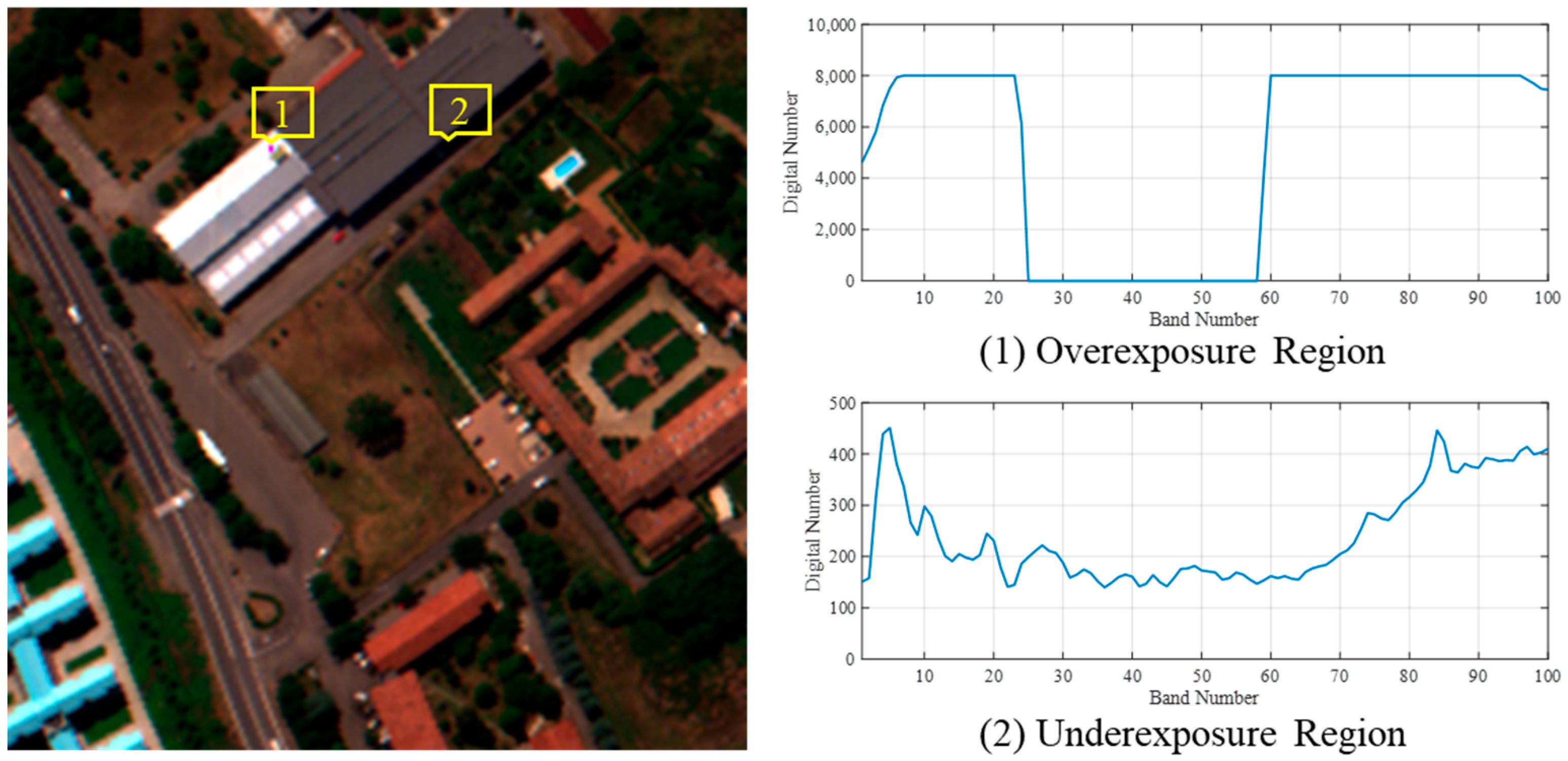
Figure 1. Extreme radiance areas in Pavia University HS datasets. In the left, yellow box 1 represents an overexposed area, and yellow box 2 represents an underexposed region. On the right side, the blue curve shows distorted spectral information.
Remotesensing 16 01248 g001
Figure 2. Flowchart of the RECF method, mainly divided into two parts, underexposed compensation and overexposed compensation.
Remotesensing 16 01248 g002
Figure 3. Error map of proposed RECF.
Remotesensing 16 01248 g003
Figure 4. Local smoothing constraint for the abundance matrix.
Remotesensing 16 01248 g004
Figure 5. Local smoothing constraint for the endmember matrix.
Remotesensing 16 01248 g005
Figure 6. Experimental data for the airborne hyperspectral dataset: (a,d,g) the experimental multispectral data from the Pavia University dataset; (b,e,h) the experimental hyperspectral data from the Chikusei dataset; and (c,f,i) the experimental hyperspectral data from the Xiong’an dataset with constructed overexposed and underexposed regions.
Remotesensing 16 01248 g006
Figure 7. HJ-2 satellite real in-orbit remote sensing data, where (a,c,e) are multispectral experimental data and (b,d,f) are hyperspectral experimental data.
Remotesensing 16 01248 g007aRemotesensing 16 01248 g007b
Figure 8. True color band composite image of Pavia University dataset.
Remotesensing 16 01248 g008
Figure 9. SAM maps of Pavia University dataset.
Remotesensing 16 01248 g009aRemotesensing 16 01248 g009b
Figure 10. True color band composite image of Chikusei dataset.
Remotesensing 16 01248 g010
Figure 11. SAM maps of Chikusei dataset.
Remotesensing 16 01248 g011
Figure 12. True color band composite image of the Xiong’an dataset.
Remotesensing 16 01248 g012
Figure 13. SAM maps of Xiong’an dataset.
Remotesensing 16 01248 g013
Figure 14. True color band composite image of Scene 1 from HJ-2 satellite HS/MS data fusion.
Remotesensing 16 01248 g014
Figure 15. True color band composite image of Scene 2 from HJ-2 satellite HS/MS data fusion.
Remotesensing 16 01248 g015
Figure 16. True color band composite image of Scene 3 from HJ-2 satellite HS/MS data fusion.
Remotesensing 16 01248 g016
Figure 17. Spectral curves of fused HH data in radiance extreme area: overexposed area comes from the rooftop of building in Scene 2, and underexposed area comes from the river region in Scene 3.
Remotesensing 16 01248 g017
Table 1. RECF flowchart.
 Algorithm Flowchart: Radiance Extreme Area Compensation Fusion
  Input: HS, MS, Algorithm parameters αE, αA, γE, γA, ρ
  Output: HH
  Step1: Identify and extract overexposed areas from HS as R_OE_HS
  Step2: Fusion radiance normal light region based on PSNMF
 (1)
Initialize Eh by VCA, and update Ah by (12), with Eh fixed.
 (2)
Calculate error-map between HS and Eh·Ah
 (3)
Update Em and Am by (13) and (14).
while not converge do
  (4)
Initialize Em by (5), and update Am by (14), with Em fixed.
  (5)
Update Em and Am by (13) and (14).
  (6)
Initialize Ah by (4), and update Eh by (11), with Ah fixed.
  (7)
Calculate error-map between HS and Eh·Ah
  (8)
Update Eh and Ah by (11) and (12).
end
 (9)
HH = Eh·Am.
  Step3: Compensate overexposed areas of fused HH by (15) and (16)
Table 2. Main parameters of experimental data.
DatasetsPlatformBandsResolutions (m)Image SizeScene Size
Pavia UniversityAirborne2241.3610 × 340320 × 320
ChikuseiAirborne1282.52517 × 2335320 × 320
Xiong’anAirborne250-3750 × 1580320 × 320
HJ-2 HSISatellite100482048 × 2048180 × 180
HJ-2 MSISatellite5166144 × 6144540 × 540
Table 3. Evaluation metrics on the Pavia University dataset.
MethodPavia University
PSNRSAMERGASQ2nCC
GS39.12292.96412.02090.98100.9903
GLP35.97582.20762.92900.98300.9858
SFIM34.51012.24983.44740.98000.9806
HySure37.10353.43032.63310.97760.9886
CNMF38.70762.27992.26320.98330.9921
FUSE37.52933.01782.66810.98030.9869
Lanaras37.66452.71552.33910.98060.9895
CSTF37.63322.68522.30870.80120.9878
NLSTF44.08072.37321.45780.90750.9945
SSFCNN39.93972.70741.83410.98160.9922
SSRNET41.26452.51881.71240.98440.9935
RECF44.66912.23931.45140.98660.9949
Table 4. Evaluation metrics on the Chikusei dataset.
MethodChikusei
PSNRSAMERGASQ2nCC
GS43.67152.01442.81780.97720.9897
GLP41.35361.22313.46200.98110.9868
SFIM40.49181.29533.68510.97940.9852
HySure42.22942.40633.79140.95240.9852
CNMF43.20311.59143.25150.97390.9884
FUSE41.78542.17613.48780.96980.9876
Lanaras42.83171.84813.47350.96980.9854
CSTF40.13102.03583.73860.99710.9832
NLSTF49.60901.62272.28530.99820.9916
SSFCNN39.06892.12793.17380.96540.9874
SSRNET40.18551.97243.05320.96130.9855
RECF49.98571.34162.25410.97920.9926
Table 5. Evaluation metrics on the Xiong’an dataset.
MethodXiong’an
PSNRSAMERGASQ2nCC
GS38.65500.86771.02650.94810.9905
GLP36.68750.63001.14090.96520.9878
SFIM36.06860.67251.20920.96460.9862
HySure37.09251.44161.21980.92670.9870
CNMF37.22730.80351.12610.96670.9881
FUSE37.60000.87571.17780.96220.9872
Lanaras37.72330.94580.91800.95430.9921
CSTF39.21850.86380.83340.86290.9926
NLSTF46.43140.69050.44920.95290.9975
SSFpecCNN33.93111.75991.72920.98240.9844
SSRNET33.34631.65771.95450.92090.98197
RECF47.60760.59640.37390.98440.9985
Disclaimer/Publisher’s Note: The statements, opinions and data contained in all publications are solely those of the individual author(s) and contributor(s) and not of MDPI and/or the editor(s). MDPI and/or the editor(s) disclaim responsibility for any injury to people or property resulting from any ideas, methods, instructions or products referred to in the content.