Expanded Signal to Noise Ratio Estimates for Validating Next-Generation Satellite Sensors in Oceanic, Coastal, and Inland Waters

Abstract

The launch of the NASA Plankton, Aerosol, Cloud, ocean Ecosystem (PACE) and the Surface Biology and Geology (SBG) satellite sensors will provide increased spectral resolution compared to existing platforms. These new sensors will require robust calibration and validation datasets, but existing field-based instrumentation is limited in its availability and potential for geographic coverage, particularly for coastal and inland waters, where optical complexity is substantially greater than in the open ocean. The minimum signal-to-noise ratio (SNR) is an important metric for assessing the reliability of derived biogeochemical products and their subsequent use as proxies, such as for biomass, in aquatic systems. The SNR can provide insight into whether legacy sensors can be used for algorithm development as well as calibration and validation activities for next-generation platforms. We extend our previous evaluation of SNR and associated uncertainties for representative coastal and inland targets to include the imaging sensors PRISM and AVIRIS-NG, the airborne-deployed C-AIR radiometers, and the shipboard HydroRad and HyperSAS radiometers, which were not included in the original analysis. Nearly all the assessed hyperspectral sensors fail to meet proposed criteria for SNR or uncertainty in remote sensing reflectance (R_rs) for some part of the spectrum, with the most common failures (>20% uncertainty) below 400 nm, but all the sensors were below the proposed 17.5% uncertainty for derived chlorophyll-a. Instrument suites for both in-water and airborne platforms that are capable of exceeding all the proposed thresholds for SNR and R_rs uncertainty are commercially available. Thus, there is a straightforward path to obtaining calibration and validation data for current and next-generation sensors, but the availability of suitable high spectral resolution sensors is limited.

1. Introduction

Coastal, estuarine, and inland waters are optically complex and exhibit significant spatial and temporal variability. Ocean color remote sensing imagery is often used to derive relevant biogeochemical constituents within coastal and inland waters at appropriate space and time scales [1]. Beyond basic research, such data products are used to provide information about species composition and biodiversity, water quality, carbon cycling, and biogeochemical fluxes relevant to human and ecosystem health [2]. Historically, ocean color sensors have focused on the open ocean, which is typically optically simple (Case-1 waters; [3]) and exhibits greater spatial and temporal decorrelation scales compared to coastal and inland waters. The coastal zone serves as a dynamic transition between the oceanic and terrestrial biomes. It represents approximately 20% of Earth’s surface [4] but provides the richest biodiversity and the highest fishery production, both of which are created from the highest primary production [4]. As such, it is an important target for remote sensing. Advances in satellite radiometry have greatly increased the availability of publicly available high spatial resolution data with the introduction of (e.g.) the Operational Land Imager (OLI; 30 m spatial resolution) aboard Landsat 8/9 and the MultiSpectral Instrument (MSI; 10, 30, 60 m spatial resolution) aboard Sentinel-2, while the launch of the Ocean Land Colour Instrument (OLCI) aboard Sentinel-3 provides a compromise between high spatial resolution (300 m) and more frequent return rate (~daily; [5]). Increasingly, the community of practice is now turning toward increased spectral resolution as well [6].

Water-leaving radiance (L_W(λ), µW cm⁻² nm⁻¹ sr⁻¹, or L_W) is highly variable, ranging from extremely low values for clear, deep water to very bright values in optically shallow environments near the shoreline, in turbidity plumes, or in high productivity waters. Legacy satellite missions such as SeaWiFS, MODIS, and VIIRS provide ~1 km and ~daily resolution, which is generally not adequate for the coastal ocean [7]. Next-generation missions such as PACE, deploying the Ocean Color Instrument (OCI; [8]), and the NASA Surface Biology and Geology (SBG) study [9] provide more spectral resolution as well as measurements that extend into shorter wavelengths. These shorter wavelengths, extending into the ultraviolet (UV), are useful for the following: (a) discriminating red tides [10]; (b) identifying point sources for pollution [11]; (c) improving atmospheric correction [12], particularly in turbid coastal waters [13,14]; and (d) reducing the uncertainties in derived biogeochemical parameters at discrete wavelengths [15] or as part of end-member analyses [16]. Most commercial-off-the-shelf (COTS) spectrometers and calibration/validation (cal/val) sensors, however, lack UV bands or exhibit poor UV performance [17]. All these issues make aquatic remote sensing, as well as cal/val activities, challenging.

The “classic” airborne visible infrared imaging spectrometer (AVIRIS-C) provides both high spatial (~5–60 m) and spectral (~400–2500 nm) resolution, and has until recently been the platform of choice for simulating ocean color products [17]. It has been complemented by the next-generation airborne sensor AVIRIS-Next Generation (AVIRIS-NG). Unfortunately, in-water and above-water instrumentation suitable for ground truth of high spectral resolution imagery has decreased in availability [18]. Handheld sensors such as the Malvern Panalytical ASD instruments are considered the gold standard but are not automated and are therefore incapable of providing continuous spectral data in complex environments. The Aerosol Robotic Network-Ocean Color (AERONET-OC) sensors are automated, but are typically deployed in a fixed location [19,20].

As previously described [21,22], the remote sensing of coastal and inland waters often involves compromises between optimizing the SNR and maintaining a broad dynamic range for ocean sensors, and saturation over bright targets caused by limited dynamic range is a common issue. In contrast, sensors designed primarily for land (e.g., MSI, SBG) are optimized for observing bright targets and do not saturate but suffer from poor performance (low SNR) for dark targets, i.e., clear, deep water. As a compromise, SNR recommendations are variously set at an SNR of > 100–200 for shortwave infrared (SWIR), >600 for near infrared (NIR), and > 1000 for UV to visible (VIS), i.e., UV-VIS, bands. Muller-Karger et al. [2] recommended an SNR > 800 for the UV-VIS range. Wang and Gordon [23] specifically evaluated NIR and SWIR bands for atmospheric correction, and identified minimum requirements of ~200–300 for NIR and ~100 for SWIR, concluding that an SNR of ~600 and ~200 for NIR and SWIR are acceptable minimum thresholds. SNR values listed for at-sensor radiances can be difficult to interpret because of the wide dynamic range of typical at-sensor radiance (L_typ) values, particularly for coastal and inland waters, and [21] recommended presenting values in terms of L_W, remote sensing reflectance (R_rs, sr⁻¹), or water-leaving reflectance (ρ_W), consistent with the PACE Science Definition Team report [24].

The goals of this manuscript are, first, to update [21] with sensors that were not included in the original analysis, in particular AVIRIS-NG. Second, this paper assesses whether existing commercially available airborne and in-water instrumentation provides sufficiently high-quality estimates of L_W (and therefore of R_rs and ρ_W). We provide guidelines for future cal/val instrument development to achieve an adequate SNR (and uncertainty) and, therefore, cal/val capability for next-generation sensors.

2. Materials and Methods

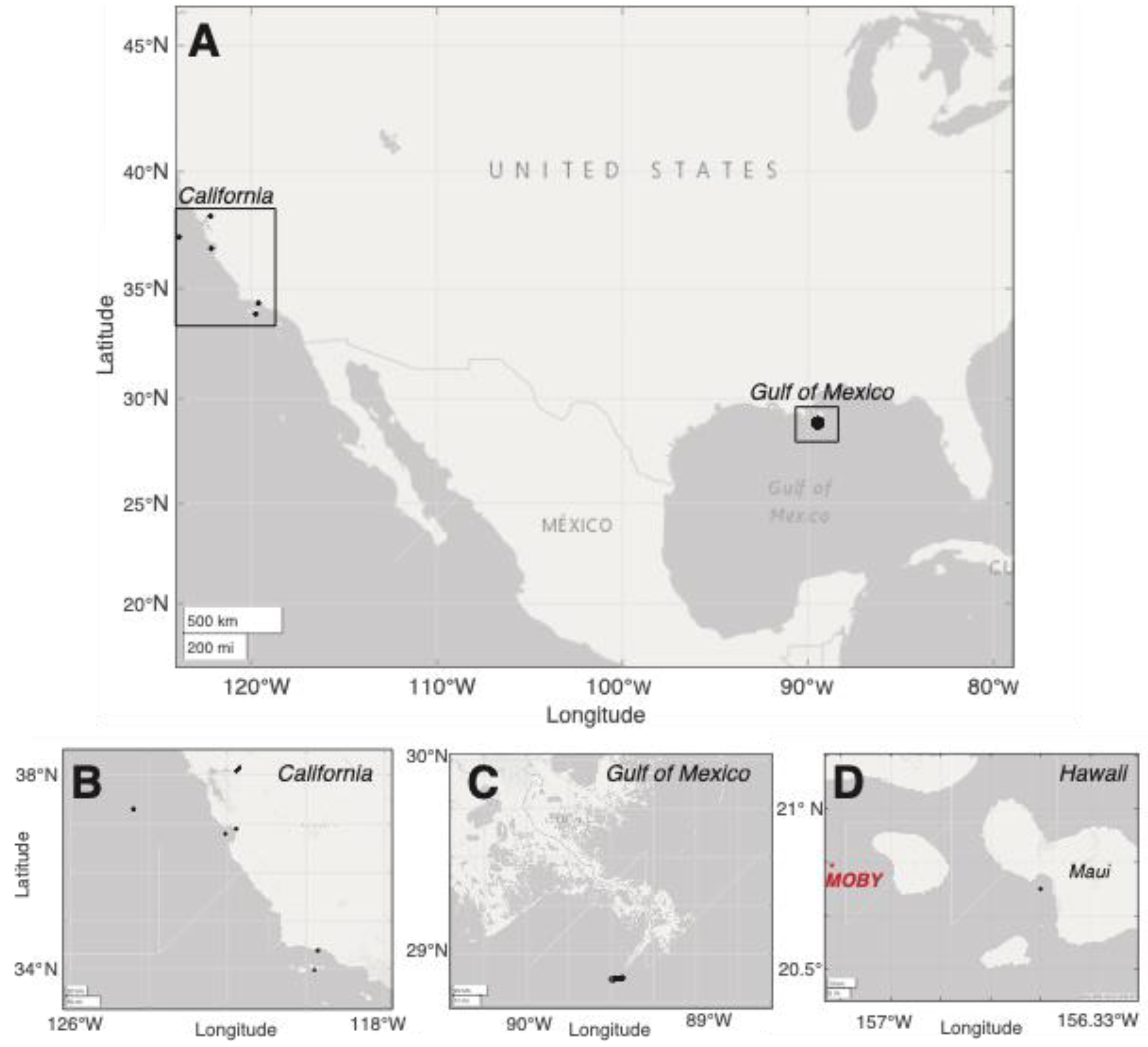
2.1. Field Sites and Targets

The sampling locations chosen for this analysis (Figure 1) were based on similar criteria as [21]. First, the sites provide L_typ values that are representative of common inland and coastal water targets; with the exception of kelp, all the targets were spatially uniform water targets referred to as “bright” or “dark”, i.e., waters with enhanced scattering (bright) or absorption (dark). Second, quality-controlled data are available (see references in Section 2), and the sites are characterized well enough to assess their use as case studies for coastal and inland ocean color remote sensing. Third, the sites are both spatially extensive and optically homogenous for applying geostatistical methods to calculate the SNR [21,25,26]. Finally, datasets were excluded that were redundant with the previous analysis [21]. Based on those criteria, we identified five relevant sites as follows: San Francisco Bay, the Sub-Mesoscale Ocean Dynamics Experiment (S-MODE) site offshore of San Francisco, coastal Monterey Bay and Elkhorn Slough, the Santa Barbara Channel, the Gulf of Mexico, and coastal Hawaii (

Table 1. Summary of data collection sites and processing parameters.

Sensor	Date	Resolution (m)	Spectral Range (Resolution) nm	Atmospheric Correction
S-MODE, Monterey Bay, Elkhorn Slough
C-AIR	28-Oct-21	3.5	320–1640 (10) *	Not Necessary
PRISM	24-Jul-12	1.0	350–1054 (3.5)	ATREM
		San Francisco Bay
HydroRad-3	23-Oct-19	95.8	350–850 (1.1)	Not Necessary
		Gulf of Mexico
HyperSAS	22-Apr-09	16.2	350–800 (3.5)	Not Necessary
		Hawaii
PRISM	17-Feb-17	16.2	350–1054 (3.5)	ATREM
		Santa Barbara Channel
AVIRIS-NG	17-Apr-21	7.9	380–2510 (5)	ATREM

* fixed wavelengths at 320, 340, 380, 412, 443, 490, 510, 532, 555, 589, 625, 670, 683, 710, 780, 875, 1020, 1245, 1640 nm.

).

2.2. In-Water, Airborne, and Satellite Sensors

Three airborne and two shipboard instrument suites were evaluated, respectively, as follows: AVIRIS-NG, PRISM, and Coastal Airborne In Situ Radiometers (C-AIR); plus the HOBI Labs HydroRad-3 and SeaBird Electronics (formerly Satlantic) HyperSAS (Table 1). AVIRIS-NG and PRISM are imaging spectrometers while the remaining instruments are spectrometers or multiple-waveband radiometers. AVIRIS-NG data were collected over the Santa Barbara Channel in support of the NASA Student Airborne Research Project (SARP) activity and were acquired as Level 2 (atmospherically corrected) data from JPL (https://avirisng.jpl.nasa.gov, accessed 28 August 2023). PRISM data were obtained during the PRISM validation campaign (Moss Landing Harbor, adjacent to Elkhorn Slough; prism.jpl.nasa.gov, accessed 12 September 2023) and the NASA COral Reef Airborne Laboratory (CORAL; [27]). Data from C-AIR were obtained as part of the NASA Coastal High Acquisition Rate Radiometers for Innovative Environmental Research (C-HARRIER) campaign in collaboration with the NASA Sub-Mesoscale Ocean Dynamics Experiment (S-MODE) experiment for offshore coastal waters, Monterey Bay, and Elkhorn Slough, California. Data from San Francisco Bay collected with the HydroRad-3 were obtained from a previous analysis [25] focusing on the derivation of Total Suspended Solids (TSS). HyperSAS data were collected in the Gulf of Mexico [28] and were obtained from the NASA SeaBASS repository [29]. Three of the four instrument suites collect data along-track, while AVIRIS-NG and PRISM collect a swath. For geostatistical analyses, we treated all the sensors as along-track. For each dataset, a homogenous along-track section used for the estimation of the SNR was identified by visual inspection of radiance or reflectance data at ~555 nm to avoid obvious features such as fronts, kelp canopy edges, and shadows.

2.2.1. AVIRIS-NG Imagery

Images for the Santa Barbara Channel were obtained from the JPL AVIRIS-NG site. The data were downloaded as Level 2 (L2) reflectance with a standard atmospheric correction applied [30]. Imagery was kept at native pixel and wavelength resolution (Table 2). Two regions were identified for analysis corresponding to a bright target (kelp bed) and dark target (clear Case-1 waters to the south of Santa Cruz Island). We compared the along-track SNR to a 2-dimensional data field [21] as well as multiple along-track datasets from the same swath and the results were comparable, so only the single along-track results are presented. R_rs was calculated using the Thuillier [31] solar irradiance spectra interpolated to AVIRIS-NG wavelengths.

2.2.2. PRISM Imagery

Images for Moss Landing Harbor, adjacent to Elkhorn Slough, and coastal waters off Maui, Hawaii, were obtained from the JPL PRISM site and the CORAL site, respectively. The data were downloaded as L2 reflectance with a standard atmospheric correction applied [30]. The imagery was kept at native pixel and wavelength resolution (Table 2). Moss Landing Harbor was chosen as a bright target (elevated TSSs) and Hawaii was chosen as a dark target (clear Case-1 waters). The PRISM data exhibit “noise” due to the high spectral resolution, and the spectra and uncertainties can be improved with non-standard processing [30], but for this analysis the standard L2 data were used.

2.2.3. C-AIR Data

The C-AIR instrument suite is manufactured by Biospherical Instruments Inc. [32] and operated by NASA Ames Research Center. As part of the C-HARRIER campaign [32], the data were collected aboard a Twin Otter aircraft. C-AIR is an airborne radiometer instrument suite based on microradiometers with a flight campaign heritage since 2011. C-AIR consists of three 19-channel microradiometers [33], one fitted with a cosine collector to measure the global solar irradiance (E_s; μW cm⁻² nm⁻¹), and two radiance instruments oriented to measure the indirect sky radiance (L_i; μW cm⁻² nm⁻¹ sr⁻¹) plus the total radiance from the surface (L_T; μW cm⁻² nm⁻¹ sr⁻¹). C-AIR is similar to the Compact-Airborne Environmental Radiometers for Oceanography (C-AERO) instrument suite [21] except for less advanced hardware (and firmware) components, the lack of radiance shrouds, and a 15 Hz sampling rate rather than as fast as 30 Hz for C-AERO [34]. In addition, the C-AIR data software is less sophisticated than C-AERO, with the former data acquisition being more properly representative of non-commanded data recording. For the latter, temporally updated laboratory metadata are combined with unique ancillary sensor records. Briefly, the combination permits preprocessing corrections to reduce uncertainties in data products [35] as follows: (a) time-dependent characterizations; (b) gain-stage transitions; (c) nonreal-time serial timing; (d) illumination geometry and normalizations; (e) planar aperture tilting; and (f) environmental or field characterizations (e.g., dark currents), as appropriate. Intercalibration corrections are not applied, because the absolute calibration of each radiometer is determined independently. Postprocessing corrections are likewise most advanced for the C-AERO data acquisition software, e.g., permitting glint discretization shown to remove positive bias (brightening) in above-water radiometric observations [36]. Lowest safe altitude (LSA) flights, ~30 m above the water surface and flown in the principal plane of the Sun to mitigate glint, were used for the data collection, negating the need for a full atmospheric correction [32]. The SNR was estimated using the L_T sensor. It was not possible to calculate R_rs for C-AIR because there were insufficient resources to fully process the data in compliance with the NASA Ocean Optics Protocols [37,38,39,40,41].

2.2.4. HydroRad-3 Data

The HydroRad-3 was deployed on the R/V Peterson in San Francisco Bay [25]. The HydroRad-3 recorded continuous radiometric measurements of E_s, L_i, and L_T. As described previously [25], the optical sensors were fixed 2 m above the main deck on the bow of the ship. The sensors were oriented such that a 100–130° average solar zenith angle was maintained during the data collection. L_T was fixed 40° down from horizontal. While R_rs was calculated [25], the L_T data were used for the calculation of the SNR for consistency. The data were quality-controlled for suspect spectra [25] prior to analysis.

2.2.5. HyperSAS Data

The HyperSAS was operated aboard the R/V Cape Hatteras in the northern Gulf of Mexico as part of the GulfCarbon program [28,29]. The HyperSAS system included two HyperOCR-R radiance sensors for L_T and L_i, plus two HyperOCR irradiance sensors for measuring E_s, covering both UV (350–400 nm) and visible (400–800 nm) wavelengths. The radiometers were mounted at 8 m height (above-water) with a 90° angle relative to the ship’s heading. The L_T and L_i sensor viewing angles were 35° from the nadir and 125° from the nadir, respectively. The data were quality-controlled as described in [28]. As with the HydroRad-3, L_T was used in this analysis for consistency.

2.3. Signal-to-Noise Ratio and Uncertainty Calculations

The SNR was estimated as the ratio of the mean signal for an invariant target to the standard deviation of the signal. The methodology has previously been described in detail [21]; we reproduce that description here as a background to the analysis. For orbital or airborne sensors designed to image water, the SNR is most often measured in the laboratory, using a spectrally uniform albedo of 5%, a reasonable reflectance for most aquatic targets [42]. Estimates of the SNR convolve multiple sources of uncertainty (noise). This can include instrument artifacts and uncertainties identified as part of the lab-based characterization of an instrument (discussed in greater detail by [43]). An alternative method, referred to as “geostatistical SNR”, calculates a semivariogram from field data that are spatially uniform. This provides an SNR that is relevant to the investigator [26] and can incorporate any pre- and post-processing, such as atmospheric correction schemes and any data reduction or quality control, if applicable. Semivariogram analysis requires that the data exhibit both isotropy and stationarity, and it is assumed that the data do not change spatial resolution [26]. The airborne data collection was at fixed altitude while the shipboard instruments were in fixed geometry relative to the target, but the assumption of isotropy may not have been rigorously met for all data. For the imaging sensors (AVIRIS-NG, PRISM), this was mitigated by testing for isotropy using the two-dimensional data, while explicitly using along-track data for analysis to be consistent across sensors. For the point-based sensors, it is not possible to test for isotropy without collecting data in multiple orientations. Since those data are not available, we analyzed multiple line segments and chose data that were qualitatively and quantitatively most uniform (see Section 2.2).

We applied a geostatistical SNR approach, generally following the methodology outlined in [25]. The SNR was determined for each wavelength by calculating the semivariance, ${\mathsf{\gamma }}_h$, over the distance between pixel pairs (h) using the MATLAB (Mathworks Inc.) packages variogram and variogramfit [44]. A theoretical semivariogram was calculated with the data to estimate the nugget, sill, and range (c.f. [25,45]). The SNR was then calculated as the mean signal ($\overline{z},$L_T or reflectance) divided by the square root of the nugget variance (C₀):

$$\mathrm{SNR}=\frac{\overline{\mathrm{z}}}{\sqrt{C_0}}.$$

(1)

The nugget (n, or C₀) is the non-zero intercept, and it determines the degree of unresolved variability, or noise. Mathematically, this is the non-zero limit of ${\mathsf{\gamma }}_h$ when h approaches zero, where h is the lag and ${\mathsf{\gamma }}_h$ is the semivariance as a function of the lag. The range (a) determines how quickly in space the variability reaches a global maximum, while the sill (C₁) indicates the point beyond which pixel proximity does not correlate with the spatial structure of the data. This provides the total resolved variance. Multiple theoretical variogram models are available and the choice of model depends on the structure of the data. For this analysis, three theoretical models were used and are formulated as:

$${\gamma }_h={C_0+C}_1[1–\exp \left(–\frac{h^2}{{\mathrm{a}}^2}\right)]$$

(2)

$${\gamma }_h={C_0+C}_1[1–\exp \left(–\frac{h}{\mathrm{a}}\right)]$$

(3)

$${\gamma }_h=\left\{\begin{array}{c}{C_0+C}_1\left(\frac{h}{\mathrm{a}}\right), h\le \mathrm{a}\\ {C_0+C}_1, h>\mathrm{a}\end{array}\right.$$

(4)

where (2) is a Gaussian, (3) is an exponential, and (4) is a bounded linear model. Following [25], the best R² value of the fit was used to select the model. Data were discarded for R² < 0.7 for all but the HyperSAS data, where the criteria had to be relaxed to < 0.5 to cover the full spectral range. For sensors other than HyperSAS the R² values exceeded 0.8–0.9 on average.

2.4. Uncertainties in R_rs and Derived Geophysical Products

For a comparison to [21], we multiplied the percent noise of the mean signal by the R_rs uncertainty for the HydroRad-3, HyperSAS, PRISM, and AVIRIS-NG (C-AIR was excluded because R_rs was not calculated). Following [21,46], the same weightings in a 3-band configuration were used for calculating chlorophyll-a (chla) from the HydroRad-3, HyperSAS, and AVIRIS-NG (dark target). For kelp, the normalized difference vegetation index (NDVI) was calculated using AVIRIS-NG (bright target). The relevant algorithms are:

$${\log }_{10}\left(chla\right)={\mathrm{a}}_0+\sum _{\mathrm{i}}^4{\mathrm{a}}_{\mathrm{i}}\left[{\log }_{10}(R_{bg}\right)]$$

(5)

where $R_{bg}$ is the ratio of maximum blue to green reflectance, and a₀–a₄ are weighting functions for instrument-specific bands (c.f. [47,48,49,50]) and for NDVI,

$$\mathrm{NDVI}=(R_{\mathrm{r}\mathrm{s}}^{NIR} - R_{\mathrm{r}\mathrm{s}}^{red})/(R_{\mathrm{r}\mathrm{s}}^{NIR}+R_{\mathrm{r}\mathrm{s}}^{red})$$

(6)

where $R_{\mathrm{r}\mathrm{s}}^{red}$, $R_{\mathrm{r}\mathrm{s}}^{NIR}$ are the remote sensing reflectances from AVIRIS-NG at 652.55 nm (red) and 852.89 nm (NIR). Uncertainty was propagated using the standard OC3M band-ratio algorithm for chlorophyll retrievals following [43], and for NDVI for the kelp target following [21], where $\delta chla$ and $\delta NDVI$ are the calculated uncertainties with units of mg m⁻³ for chla and dimensionless units (−1 to 1) for NDVI.

3. Results

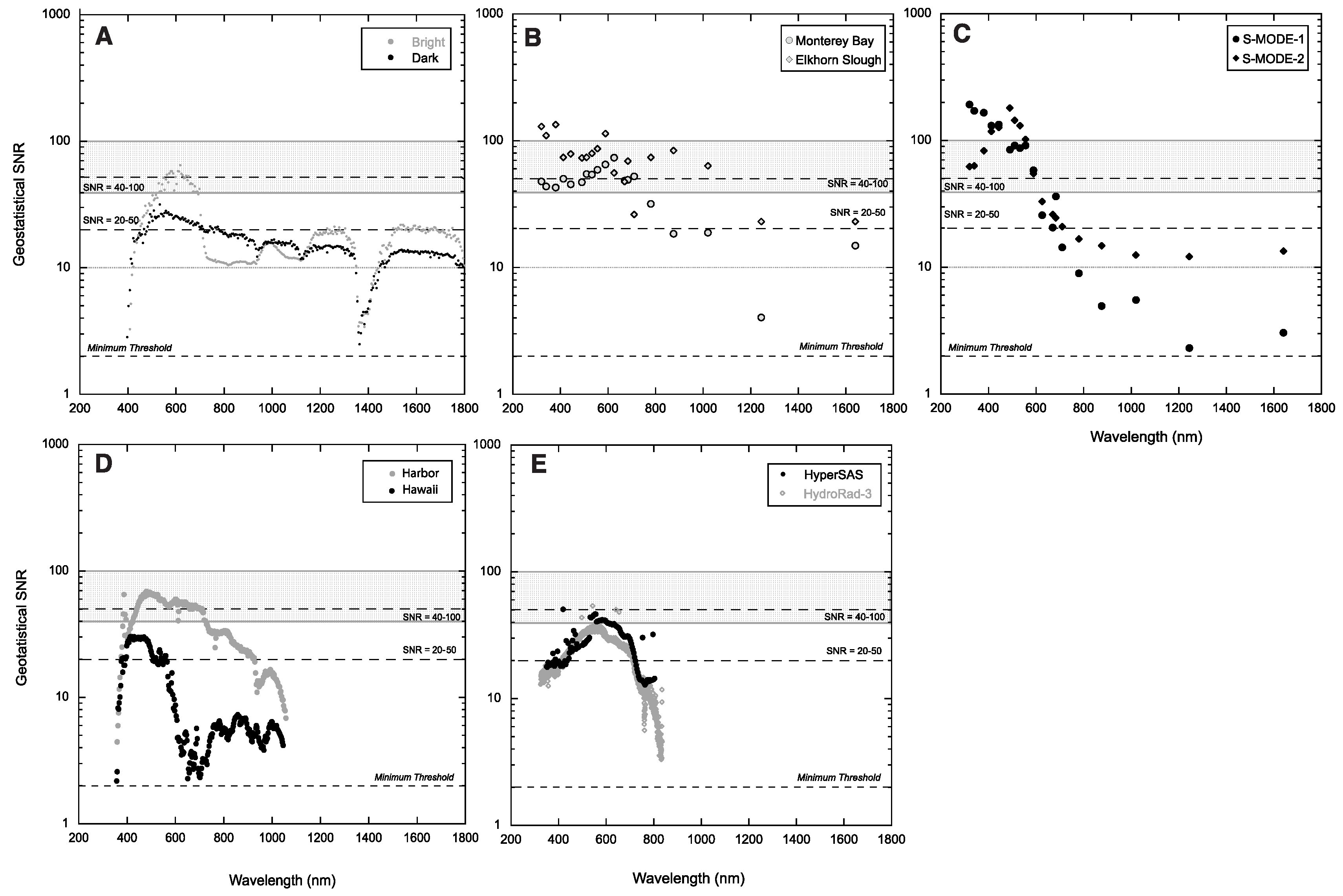
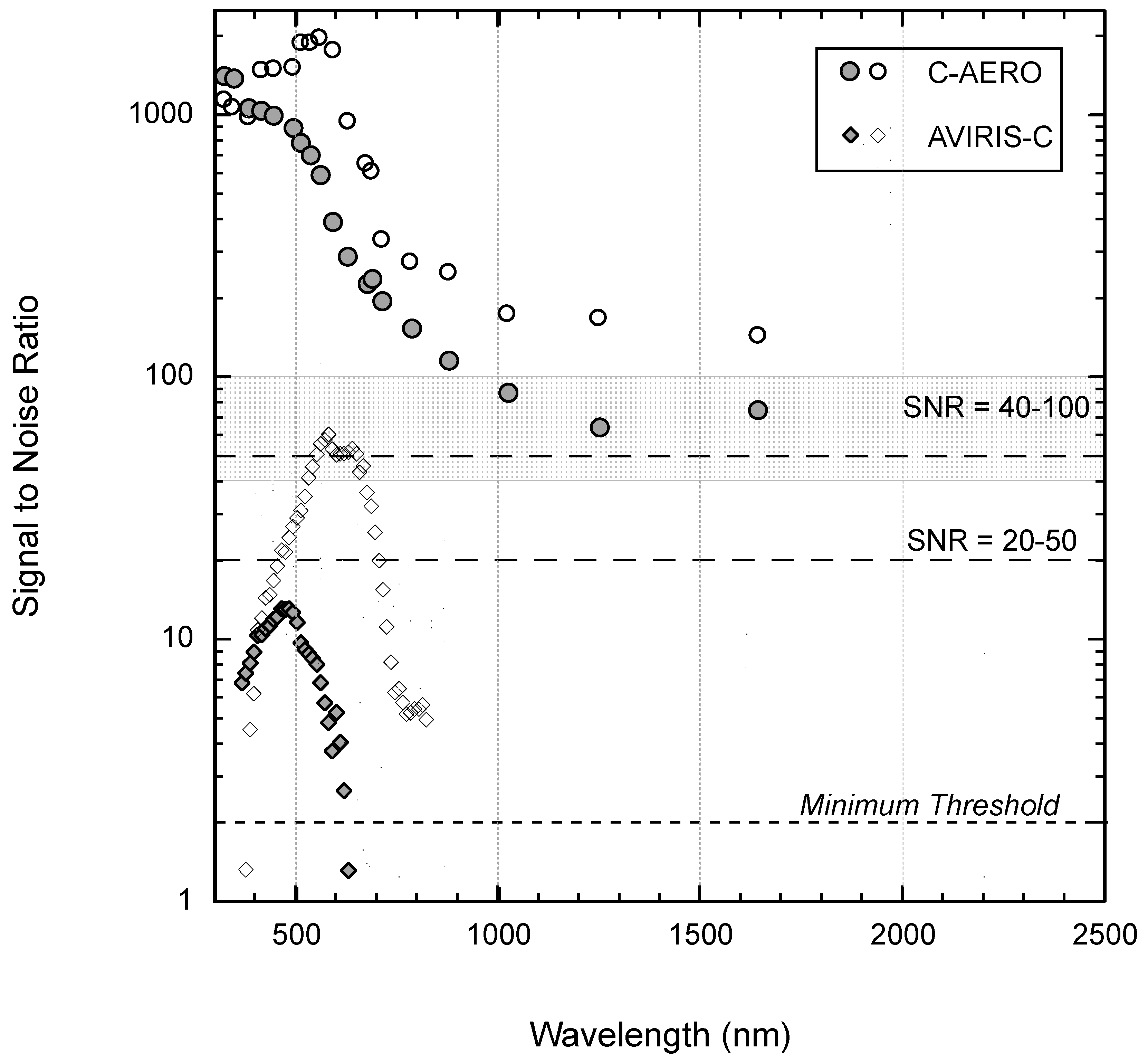
3.1. Geostatistical SNR

Previous analysis [21] provided SNR estimates for multiple satellite and airborne sensors for comparison to AVIRIS-NG, PRISM, C-AIR, HydroRad-3, and HyperSAS. Figure 2 shows a subset of those results for AVIRIS-C and C-AERO. C-AERO exhibited the highest SNR and lowest uncertainty across all wavelengths. AVIRIS-C exhibited rapid declines below ~450 nm and above ~700 nm with a peak SNR between ~490–700 nm depending on the target. As discussed in [21], an SNR of two provides the absolute minimum threshold for scientifically relevant data. The at-sensor signal for aquatic targets is assumed to be ~5% of L_typ. Therefore, for an at-sensor SNR of 400–1000, the atmospherically corrected SNR should be 20–50. Doubling those values to account for other sources of variance results in a minimum SNR of 40–100. Figure 2 thus provides examples of an airborne sensor that meets proposed standards (C-AERO) and an airborne sensor (AVIRIS-C) that does not consistently meet proposed standards.

Figure 3 provides the corresponding SNR for the airborne and shipboard datasets included in this analysis. AVIRIS-NG exhibits higher SNR compared to AVIRIS-C, but still falls below a threshold of 20 for blue-UV (<~450 nm) and for wavelengths beyond 750 nm, although those bands are of less interest for ocean color (but see [51]). C-AIR is consistently above both SNR thresholds in the UV and visible bands, but also drops off for wavelengths beyond 750 nm, particularly for dark targets (e.g., S-MODE). C-AIR exhibits about a decade of loss in the SNR compared to C-AERO. For the two shipboard sensors, the SNR peaks at ~555 nm, just at or below the proposed SNR threshold of 20. The SNR continues to drop into the UV and the NIR ranges.

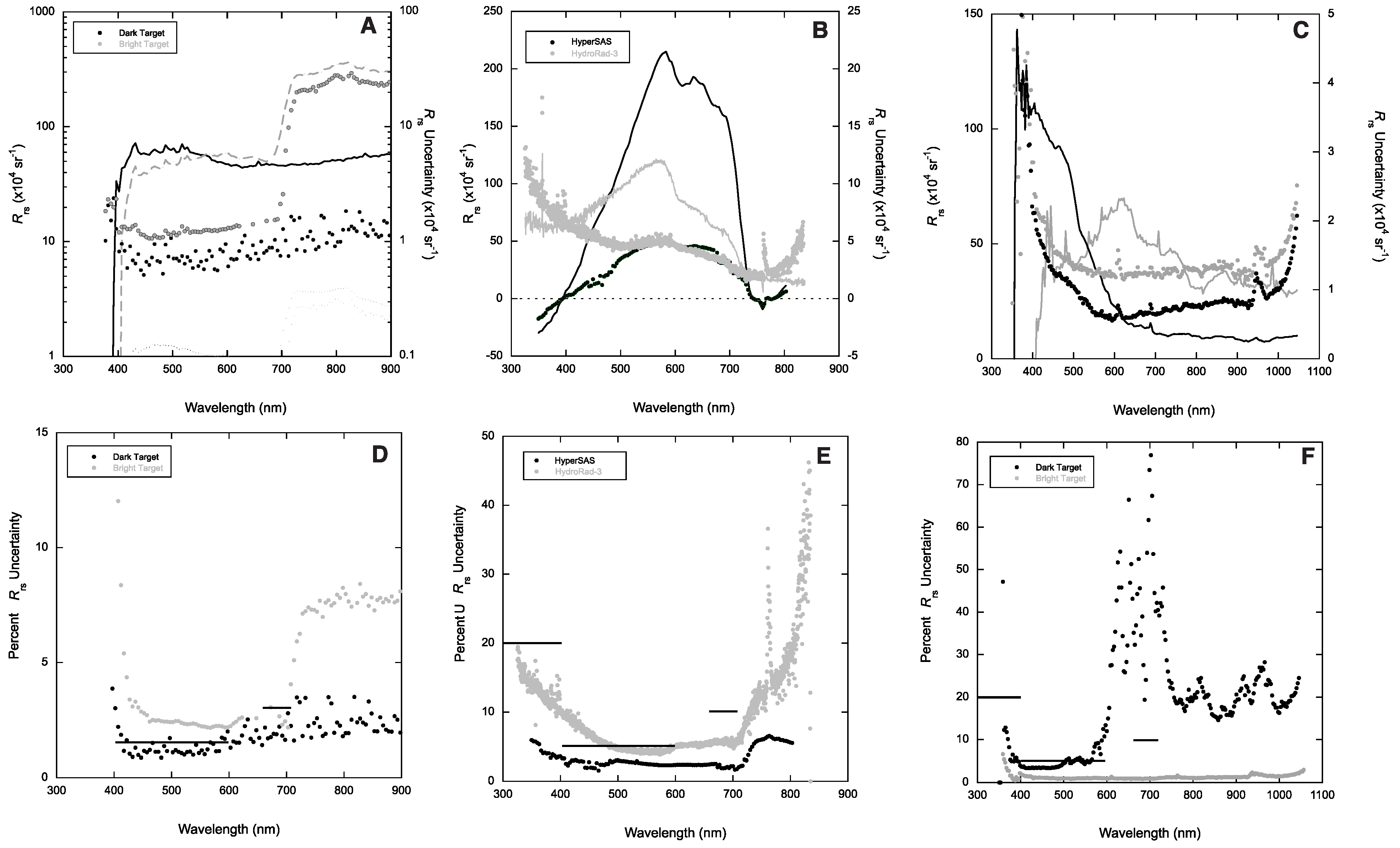
3.2. Airborne and Satellite-Derived Uncertainty

Figure 4 provides the R_rs spectra and corresponding data for AVIRIS-NG, PRISM, HyperSAS, and HydroRad-3 as R_rs and uncertainty (sr⁻¹), and as percent environmental uncertainty. C-AIR was excluded because R_rs was not available, but the results from [21] provide a reasonable estimate of C-AIR instrument uncertainty. Hooker et al. [52] provide guidelines for the generalized spectral properties of dark and bright water bodies in terms of peaks and spectral end members as follows: (1) a radiometrically dark water body has a central peak spanning the blue–green domains with the lesser amplitudes at shorter wavelengths containing secondary features and the substantially decreasing amplitudes at longer wavelengths containing an identifiable fluorescence peak in the red domain; and (2) a radiometrically bright water body has a dominant peak shifted toward the red–NIR domains with a usually identifiable fluorescence peak, plus secondary features (including lesser peaks) at shorter wavelengths, wherein with respect to a dark water body, the shortest wavelengths have significantly reduced amplitudes, but the longest wavelengths have elevated amplitudes. The generalized properties of dark and bright water bodies are not applicable to all the sampling circumstances and are provided to assist the reader in generally assessing the material provided in the figures without the need to state all the discernible features within or between figures. Consequently, only the most important differences relevant to the study are described below.

The PACE Science Definition team specified percent uncertainty ranges of 20% for 350–400 nm, 5% for 400–600 nm, and 10% for 660–710 nm [24]. AVIRIS-NG does not provide data from 350 to 400 nm and was generally below the thresholds for dark targets, but not for bright targets. PRISM does extend below 400 nm for the dark (but not bright) target and is below the 20% proposed uncertainty threshold, but exhibits variability in the UV range. In the visible spectrum, PRISM is not compliant for the dark target and fails the proposed threshold from ~400–450 nm for the bright target. HydroRad-3 was generally in compliance, except for the ~400–500 nm wavelengths. HyperSAS was well below the proposed thresholds for all the wavelengths, but exhibited negative reflectances below ~400 nm.

The R_rs spectra were consistent with the expected targets; the PRISM and AVIRIS-NG dark (blue water) spectra peaked in the blue and steadily declined into the red and NIR ranges, while the bright (kelp) target exhibited a strong red edge feature from the surface canopy of the kelp bed. The Moss Landing Harbor, San Francisco Bay, and Gulf of Mexico targets (bright) exhibited very high R_rs peaking between 550 and 600 nm, consistent with sediment-laden waters [25,28].

There was an unusual pattern in the AVIRIS-NG uncertainty, with both the absolute uncertainty and percent uncertainty rising in the red edge feature over the kelp, tracking the R_rs signal. While still below the PACE-specified threshold, it suggests that despite choosing an apparently homogenous section of the kelp bed, there was pixel or subpixel variability that influenced the variogram. This is presumably due to the high spatial heterogeneity (e.g., [45]) associated with kelp beds at the native spatial resolution of AVIRIS-NG from this data collection. PRISM also showed spectral variability at some wavelengths consistent with narrow spectral bands being influenced by atmospheric absorption features [30] that tend to be smoothed out in lower spectral resolution data.

3.3. Derived Chlorophyll and NDVI

AVIRIS-NG and PRISM data were converted to R_rs and HydroRad-3 and HyperSAS R_rs were used to calculate chla and NDVI (for kelp). Although fully quality-controlled R_rs were not available for C-AIR, we calculated $\delta chla$ for the C-AIR dark targets (S-MODE) using a simplified above-water correction scheme following [47] with ρ = 0.028. Corresponding R_rs uncertainties are not provided (as noted above) given the simplified correction, but the analysis provides a first-order estimate of instrument uncertainty for $\delta chla$ using C-AIR over a dark target.

In-water validation data were not available for all the sites, so $\delta chla$ and $\delta NDVI$ are presented as percent uncertainty due to the estimated error introduced to the algorithm (OC3M or NDVI) associated with environmental variability and instrument performance, referred to hereafter as environmental uncertainty (U_E, %). Reported U_E is, therefore, only an indication of the sensor performance as deployed and processed and does not account for potential uncertainties or biases in the underlying algorithm, nor does it capture total uncertainty. Statistics that compare satellite vs. in situ matchups result in a considerably higher mean error. For example, [49] reported an ~11% error for chla in the California Current (where in situ is considered correct), while [50] reported a Mean Absolute Error for OC3 applied to global MODIS matchups of 1.64, or about a 64% error.

For C-AERO, direct matchups between airborne and in situ data were available, while for San Francisco Bay and the Gulf of Mexico, in-water data that were spatially and temporally close but not true matchups were available. Those values provide U_E between 8.1 and 55.2% (relative percent difference), respectively, comparable to [50]. With those caveats, Table 2 provides results from the relevant sensors. Kudela et al. [21] proposed a first-order threshold of between 2.5 and 17.5% uncertainty of the underlying algorithm for optically complex coastal and inland waters. With the exception of AVIRIS-C for $\delta chla$, all the sensors were under the relevant thresholds for U_E. The data demonstrate that U_E generally tracks kelp health (more positive NDVI), with increasing uncertainty as NDVI values decrease. In contrast, for chla, there is no clear relationship between biomass and U_E, with performance more closely associated with the sensor rather than environmental conditions. Of the sensors evaluated, C-AERO exhibited the highest SNR and lowest absolute R_rs uncertainty metrics, with C-AIR providing quantitatively similar performance for $\delta chla \mathrm{o}\mathrm{v}\mathrm{e}\mathrm{r} \mathrm{a} \mathrm{d}\mathrm{a}\mathrm{r}\mathrm{k} \mathrm{t}\mathrm{a}\mathrm{r}\mathrm{g}\mathrm{e}\mathrm{t}$. AVIRIS-NG exhibited lower uncertainty for $\delta chla$ but not $\delta NDVI$ compared to AVIRIS-C. PRISM showed increasing U_E for the dark target. All sensors except AVIRIS-C were below the proposed threshold of 17.5% U_E.

Table 2. Summary statistics for instrument uncertainty in retrieved biomass. OC3M estimates for chla were classified for eutrophic status based on [50]. Measured chla (mg m⁻³), when available, are included in parentheses.

Location	Sensor	Algorithm	UE (%)	Biomass (NDVI, chla)	Source
Santa Barbara Channel	AVIRIS-NG	NDVI	5.4	0.57	This Study
Santa Barbara Channel	AVIRIS-C	NDVI	0.7	0.97	[21]
Santa Barbara Channel	OLI	NDVI	0.9	0.80	[21]
Santa Barbara Channel	MSI	NDVI	8.2	0.34	[21]
Santa Barbara Channel	RapidEye-2	NDVI	4.1	0.82	[21]
Santa Barbara Channel	AVIRIS-NG	OC3M	2.4	1.17	This Study
Moss Landing Harbor	PRISM	OC3M	0.7	3.66	This Study
Maui, Hawaii	PRISM	OC3M	1.3	0.31	This Study
San Francisco Bay	C-AERO	OC3M	0.1	8.08 (9.19)	[21]
Lake Tahoe	C-AERO	OC3M	0.2	0.49 (0.44)	[21]
Central California (S-MODE)	C-AIR	OC3M	0.2	0.21	This Study
San Francisco Bay	OLCI	OC3M	1.1	17.71	[21]
San Francisco Bay	AVIRIS-C	OC3M	40	3.58	[21]
San Francisco Bay	OLI	OC3M	1.1	2.75	[21]
San Francisco Bay	MSI	OC3M	4.1	3.52	[21]
Gulf of Mexico	HyperSAS	OC3M	2.3	1.90 (3.35)	This Study
San Francisco Bay	HydroRad-3	OC3M	10.5	2.84 (2.62)	This Study

Table 2. Summary statistics for instrument uncertainty in retrieved biomass. OC3M estimates for chla were classified for eutrophic status based on [50]. Measured chla (mg m⁻³), when available, are included in parentheses.

Location	Sensor	Algorithm	UE (%)	Biomass (NDVI, chla)	Source
Santa Barbara Channel	AVIRIS-NG	NDVI	5.4	0.57	This Study
Santa Barbara Channel	AVIRIS-C	NDVI	0.7	0.97	[21]
Santa Barbara Channel	OLI	NDVI	0.9	0.80	[21]
Santa Barbara Channel	MSI	NDVI	8.2	0.34	[21]
Santa Barbara Channel	RapidEye-2	NDVI	4.1	0.82	[21]
Santa Barbara Channel	AVIRIS-NG	OC3M	2.4	1.17	This Study
Moss Landing Harbor	PRISM	OC3M	0.7	3.66	This Study
Maui, Hawaii	PRISM	OC3M	1.3	0.31	This Study
San Francisco Bay	C-AERO	OC3M	0.1	8.08 (9.19)	[21]
Lake Tahoe	C-AERO	OC3M	0.2	0.49 (0.44)	[21]
Central California (S-MODE)	C-AIR	OC3M	0.2	0.21	This Study
San Francisco Bay	OLCI	OC3M	1.1	17.71	[21]
San Francisco Bay	AVIRIS-C	OC3M	40	3.58	[21]
San Francisco Bay	OLI	OC3M	1.1	2.75	[21]
San Francisco Bay	MSI	OC3M	4.1	3.52	[21]
Gulf of Mexico	HyperSAS	OC3M	2.3	1.90 (3.35)	This Study
San Francisco Bay	HydroRad-3	OC3M	10.5	2.84 (2.62)	This Study

4. Discussion

We updated the results from [21] to include current state-of-the-art imaging spectrometers (AVIRIS-NG and PRISM) as well as three COTS sensors capable of providing near-continuous measurements spatially (C-AIR, HyperSAS, HydroRad-3). In evaluating these and other sensors, one criterion for choosing to use a sensor is whether its performance is fit for purpose [15]. Ocean color remote sensing (broadly defined to include all aquatic remote sensing but referred to as “ocean color” for convenience) can be divided into three categories: calibration, validation, and research (CVR; [32,35]). Calibration has usually relied on fixed-location, custom-built radiometers at specific locations, e.g., MOBY [48], but Bouée pour l’acquisition de Séries Optiques à Long Terme (BOUSSOLE) used COTS radiometers [53]. Mobile autonomous platforms that meet calibration quality standards while extending observations into the UV and SWIR have also been demonstrated [35]. Requirements for validation are generally less rigorous and extend measurements to include both custom-built and COTS instrumentation including fixed platform [19], airborne [32], shipboard [11,54], and autonomous vehicles [35,55]. Research quality observations are the least restrictive and represent the vast majority of ocean color measurements. For calibration and validation, there are considerably fewer hyperspectral data, and even fewer data that extend into the UV [56,57] and SWIR [43] ranges.

Next-generation sensors extend observations into the UV range, primarily to improve atmospheric correction [12], although, as noted in the introduction, there are multiple biogeochemical parameters of interest that take advantage of UV bands [10,15,16,58,59,60]. While fixed-location UV sensors suitable for ocean color validation exist [11,48], the use of airborne, autonomous vehicle, or automated shipboard platforms for CVR exercises enables increased spatial extent at the temporal scale needed for match-ups to satellite observations as well as for characterizing dynamic, optically complex environments [32,35,52,55,61]. AVIRIS-C, AVIRIS-NG, and HyperSAS exhibit poor performance or lack data (either because of atmospheric correction failure or lack of bands) in the UV range. C-AIR, C-AERO, PRISM (for dark targets), and HydroRad-3 provide reasonable data (based on SNR, R_rs uncertainty) but are of limited availability. The community of practice would benefit from access to, and support for, sensors with high UV fidelity that also provide adequate spatial and temporal coverage. At the other end of the spectrum, short-wave infrared bands are also underutilized. A recent analysis demonstrates that the technology used in C-AIR and C-AERO is fully capable of delivering absolute radiometric measurements of targets darker than sunlit waters (Figure 2 and Figure 3A,D), and negating the common assumption of a “black pixel” in the NIR or SWIR region of the spectrum [51]. If the community of practice were to take advantage of those wavelengths, similar issues as for the UV bands become evident.

An instrument that meets calibration-quality performance is automatically capable of validation and research-level performance. Microradiometer technology has met this threshold [35] for in-water instruments and C-AERO is arguably also of calibration quality (Figure 2). C-AIR is based on the same technology but exhibits a lower SNR for the NIR and SWIR wavelengths (Figure 2), effectively placing it into the validation-quality category. AVIRIS-NG exhibit validation-quality performance, while HyperSAS and HydroRad-3 also meet the requirements for most wavelengths. Kudela et al. [21] noted that operational validation is possible for several sensors over turbid waters or for a reduced spectral range over blue or turbid waters (PRISM, MSI, OLCI, OLI, AVIRIS-C), to which we can add C-AIR, HyperSAS, and HydroRad-3. For dark targets, the available sensors for validation are limited if the full hyperspectral (UV-SWIR) range is required. Only C-AERO meets or exceeds all the proposed criteria, but it is multispectral rather than hyperspectral. Many of the sensors fail in the UV range. HydroRad-3 (at least in this analysis) shows a degraded performance from ~400–450 nm for a bright target, which would potentially translate to poor performance for dark targets as well. For all sensors, performance can be improved with spatial or spectral binning [62,63,64,65], but that negates the value of sensors with high spectral and spatial resolution [2].

For research, a reasonable criterion is that derived biogeochemical variables such as chla and NDVI exhibit better than 17.5% U_E for typical environments. While this study is limited in the number of targets, all the sensors meet this threshold, presumably in part because, as noted in [21], objectively poor (radiometrically) sensors often provide robust biogeochemical estimates when using band-ratio algorithms. Numerous publications have successfully applied all of these sensors to both inland and coastal waters, and the relative insensitivity of band-ratio algorithms to spatial and spectral resolution as well as radiometric performance is encouraging, providing a basis for the use of less expensive and lower performance sensors on novel platforms such as unoccupied airborne vehicles [6].

A question that is increasingly being asked is whether hyperspectral measurements are required or desirable for operational aquatic remote sensing [6]. While valuable, the large data volume [66] and corresponding field validation data [67] present challenges. There are anticipated benefits such as the ability to identify specific spectral signatures for (e.g.) phytoplankton groups [68,69] or trace gasses such as methane [70,71], but a more common use is to locally tune band-ratio algorithms to achieve better performance [72,73] or to track spectrally dynamic features such as fluorescence line height [74] using a subset of fixed wavelengths. Recent analysis shows that global ocean hyperspectral data have comparable degrees of freedom compared to legacy sensors such as MODIS because of strong covariance across wavelengths [75]. While this may set an upper limit on the number of parameters that can be independently extracted from hyperspectral imagery, it does not negate the use-case for the identification of spectrally narrow features or for band-switching algorithms. Nonetheless, the launch of PACE and SBG and the lack of readily available validation-quality hyperspectral instrumentation that can collect data at relevant spatial and temporal scales for inland and coastal waters is problematic. One potential solution is to combine high-fidelity multiwavelength point measurements with spectrometers [35] or to rely on numerical models to recreate full spectral data [76,77]. A third approach would be to rely on a variety of sensors with varying performance characteristics deployed as a sensor web [32,78,79].

This analysis focused exclusively on sensors amenable to the geostatistical determination of the SNR, which precludes the inclusion of fixed-location sensors [19] and in-water sensors on a variety of platforms [11,35,55]. While not discussed, it is implicit in proposed PACE validation activities that airborne sensors would be complemented with fixed-position, shipboard, and autonomous platforms [80]; the same validation methodology would also serve for other imminent hyperspectral missions [81]. This multi-modality approach has many advantages, including capturing a wider range of remote sensing targets than are available from calibration sites, the potential for improved R_rs uncertainty [30] and cross-validation of airborne and in-water sensors [32], particularly for sensor web configurations. This analysis provides SNR and R_rs uncertainty metrics for the sensors as used, which are often greatly degraded compared to ideal (engineering) estimates under controlled conditions. For example, PRISM is reported to have an SNR of 500 at 450 nm [80] while AVIRIS-NG was reported to have an SNR of 54–1114 (average of 345) for a scene-derived SNR from terrestrial targets [82]. In contrast, the estimates of HyperSAS R_rs uncertainty of 10–15% under typical field conditions [82] were comparable to the HyperSAS and HydroRad-3 results from this analysis (Table 2).

The apparent discrepancy between the realized geostatistical SNR and ideal SNR can be caused by numerous factors since there are many sources of error such as instrument (hardware) noise, environmental variability, and incomplete or insufficient post-processing, e.g., incomplete removal of skylight and glint contamination. Data collection that follows existing protocols will reduce errors even for high-fidelity instruments. As an example, Figure 2 provides the SNR for dark and bright targets using C-AERO with data collection that followed strict metrology. Figure 3B,C provide the SNR for C-AIR over comparable dark and bright targets. The underlying hardware is essentially identical as used (the same sampling rate was used for both data collections), other than the inclusion of shrouds on C-AERO, which should reduce noise in the SWIR. The realized SNR is about an order of magnitude lower for C-AIR compared to C-AERO for the same geostatistical analysis, suggesting that the discrepancy is largely associated with the data collection (i.e., metrology), acquisition software, and post-processing; in the case of C-AIR for this study, support was available for data collection but not for full post-processing, highlighting the need for better end-to-end support for airborne missions to improve collection of high quality data.

Looking into the near future, this analysis demonstrates that next-generation remote sensing satellite platforms would benefit from next-generation calibration and validation technology given that existing instrumentation is of limited availability or no longer supported by the manufacturers. This has minor impacts on band-ratio based algorithms but suggests that the ocean color community is lacking in commercially available sensors (other than fixed-position deployments) that can provide adequate calibration and validation data across the full spectral range. While this issue is minimized for global ocean color, science assessing inland and coastal waters will suffer unnecessarily due to the lack of high-fidelity cal/val data.

5. Conclusions

We update a previous analysis of multiple sensors to demonstrate that presently operational shipboard, airborne, and satellite sensors are effective in the SNR and R_rs uncertainty for typical coastal and inland targets. C-AERO continues to provide the highest SNR and lowest R_rs uncertainties. AVIRIS-NG performs very well for aquatic targets but does not reach validation-quality data for all wavelengths at native resolution. Neither AVIRIS-NG nor PRISM can reliably provide data at the specified accuracy in the UV range. The derived biogeochemical products such as chla and NDVI are remarkably tolerant to poor radiometric performance and are retrieved with compliant accuracy for environmental uncertainty. Existing COTS technology (C-AERO) exceeds all radiometric requirements for the calibration and validation of multi-wavelength sensors extending into the UV, NIR, and SWIR ranges, while also exceeding all criteria for application to the clearest (darkest) inland (e.g., Lake Tahoe) and open-ocean systems.

References

1. Sathyendranath, S. (Ed.) Remote Sensing of Ocean Colour in Coastal, and Other Optically-Complex, Waters; International Ocean-Colour Coordinating Group: Dartmouth, NS, Canada, 2000. [Google Scholar]
2. Muller-Karger, F.E.; Hestir, E.; Ade, C.; Turpie, K.; Roberts, D.A.; Siegel, D.; Miller, R.J.; Humm, D.; Izenberg, N.; Keller, M.; et al. Satellite Sensor Requirements for Monitoring Essential Biodiversity Variables of Coastal Ecosystems. Ecol. Appl. 2018, 28, 749–760. [Google Scholar] [CrossRef] [PubMed]
3. Morel, A.; Prieur, L. Analysis of Variations in Ocean Color1: Ocean Color Analysis. Limnol. Oceanogr. 1977, 22, 709–722. [Google Scholar] [CrossRef]
4. Crossland, C.J.; Baird, D.; Ducrotoy, J.-P.; Lindeboom, H.; Buddemeier, R.W.; Dennison, W.C.; Maxwell, B.A.; Smith, S.V.; Swaney, D.P. The Coastal Zone—A Domain of Global Interactions. In Coastal Fluxes in the Anthropocene; Crossland, C.J., Kremer, H.H., Lindeboom, H.J., Marshall Crossland, J.I., Le Tissier, M.D.A., Eds.; Global Change—The IGBP Series; Springer: Berlin/Heidelberg, Germany, 2005; pp. 1–37. ISBN 978-3-540-25450-8. [Google Scholar]
5. Donlon, C.; Berruti, B.; Buongiorno, A.; Ferreira, M.-H.; Féménias, P.; Frerick, J.; Goryl, P.; Klein, U.; Laur, H.; Mavrocordatos, C.; et al. The Global Monitoring for Environment and Security (GMES) Sentinel-3 Mission. Remote Sens. Environ. 2012, 120, 37–57. [Google Scholar] [CrossRef]
6. Dierssen, H.M.; Ackleson, S.G.; Joyce, K.E.; Hestir, E.L.; Castagna, A.; Lavender, S.; McManus, M.A. Living up to the Hype of Hyperspectral Aquatic Remote Sensing: Science, Resources and Outlook. Front. Environ. Sci. 2021, 9, 649528. [Google Scholar] [CrossRef]
7. Aurin, D.; Mannino, A.; Franz, B. Spatially Resolving Ocean Color and Sediment Dispersion in River Plumes, Coastal Systems, and Continental Shelf Waters. Remote Sens. Environ. 2013, 137, 212–225. [Google Scholar] [CrossRef]
8. Gorman, E.; Kubalak, D.A.; Deepak, P.; Dress, A.; Mott, D.B.; Meister, G.; Werdell, J. The NASA Plankton, Aerosol, Cloud, Ocean Ecosystem (PACE) Mission: An Emerging Era of Global, Hyperspectral Earth System Remote Sensing. In Proceedings of the Sensors, Systems, and Next-Generation Satellites XXIII; Neeck, S.P., Kimura, T., Martimort, P., Eds.; SPIE: Strasbourg, France, 10 October 2019; p. 15. [Google Scholar]
9. Cawse-Nicholson, K.; Townsend, P.A.; Schimel, D.; Assiri, A.M.; Blake, P.L.; Buongiorno, M.F.; Campbell, P.; Carmon, N.; Casey, K.A.; Correa-Pabón, R.E.; et al. NASA’s Surface Biology and Geology Designated Observable: A Perspective on Surface Imaging Algorithms. Remote Sens. Environ. 2021, 257, 112349. [Google Scholar] [CrossRef]
10. Kahru, M.; Anderson, C.; Barton, A.D.; Carter, M.L.; Catlett, D.; Send, U.; Sosik, H.M.; Weiss, E.L.; Mitchell, B.G. Satellite Detection of Dinoflagellate Blooms off California by UV Reflectance Ratios. Elem. Sci. Anthr. 2021, 9, 00157. [Google Scholar] [CrossRef]
11. Hooker, S.B.; Morrow, J.H.; Matsuoka, A. Apparent Optical Properties of the Canadian Beaufort Sea—Part 2: The 1% and 1 Cm Perspective in Deriving and Validating AOP Data Products. Biogeosciences 2013, 10, 4511–4527. [Google Scholar] [CrossRef]
12. Frouin, R.J.; Franz, B.A.; Ibrahim, A.; Knobelspiesse, K.; Ahmad, Z.; Cairns, B.; Chowdhary, J.; Dierssen, H.M.; Tan, J.; Dubovik, O.; et al. Atmospheric Correction of Satellite Ocean-Color Imagery During the PACE Era. Front. Earth Sci. 2019, 7, 145. [Google Scholar] [CrossRef]
13. Gao, B.-C.; Montes, M.J.; Davis, C.O.; Goetz, A.F.H. Atmospheric Correction Algorithms for Hyperspectral Remote Sensing Data of Land and Ocean. Remote Sens. Environ. 2009, 113, S17–S24. [Google Scholar] [CrossRef]
14. He, X.; Bai, Y.; Pan, D.; Tang, J.; Wang, D. Atmospheric Correction of Satellite Ocean Color Imagery Using the Ultraviolet Wavelength for Highly Turbid Waters. Opt. Express 2012, 20, 20754. [Google Scholar] [CrossRef] [PubMed]
15. Hooker, S.B.; Houskeeper, H.F.; Lind, R.N.; Suzuki, K. One- and Two-Band Sensors and Algorithms to Derive aCDOM(440) from Global Above- and In-Water Optical Observations. Sensors 2021, 21, 5384. [Google Scholar] [CrossRef] [PubMed]
16. Hooker, S.B.; Matsuoka, A.; Kudela, R.M.; Yamashita, Y.; Suzuki, K.; Houskeeper, H.F. A Global End-Member Approach to Derive aCDOM(440) from near-Surface Optical Measurements. Biogeosciences 2020, 17, 475–497. [Google Scholar] [CrossRef]
17. Hochberg, E.J.; Roberts, D.A.; Dennison, P.E.; Hulley, G.C. Special Issue on the Hyperspectral Infrared Imager (HyspIRI): Emerging Science in Terrestrial and Aquatic Ecology, Radiation Balance and Hazards. Remote Sens. Environ. 2015, 167, 1–5. [Google Scholar] [CrossRef]
18. University of Maine; Haëntjens, N.; Forsythe, K.; Denholm, B.; Loftin, J.; Boss, E. pySAS: Autonomous Solar Tracking System for Surface Water Radiometric Measurements. Oceanography 2022, 35, 55–59. [Google Scholar] [CrossRef]
19. Zibordi, G.; Holben, B.; Hooker, S.B.; Mélin, F.; Berthon, J.-F.; Slutsker, I.; Giles, D.; Vandemark, D.; Feng, H.; Rutledge, K.; et al. A Network for Standardized Ocean Color Validation Measurements. Eos Trans. AGU 2006, 87, 293. [Google Scholar] [CrossRef]
20. Zibordi, G.; Holben, B.N.; Talone, M.; D’Alimonte, D.; Slutsker, I.; Giles, D.M.; Sorokin, M.G. Advances in the Ocean Color Component of the Aerosol Robotic Network (AERONET-OC). J. Atmos. Ocean. Technol. 2021, 38, 725–746. [Google Scholar] [CrossRef]
21. Kudela, R.M.; Hooker, S.B.; Houskeeper, H.F.; McPherson, M. The Influence of Signal to Noise Ratio of Legacy Airborne and Satellite Sensors for Simulating Next-Generation Coastal and Inland Water Products. Remote Sens. 2019, 11, 2071. [Google Scholar] [CrossRef]
22. Mouw, C.B.; Hardman-Mountford, N.J.; Alvain, S.; Bracher, A.; Brewin, R.J.W.; Bricaud, A.; Ciotti, A.M.; Devred, E.; Fujiwara, A.; Hirata, T.; et al. A Consumer’s Guide to Satellite Remote Sensing of Multiple Phytoplankton Groups in the Global Ocean. Front. Mar. Sci. 2017, 4, 41. [Google Scholar] [CrossRef]
23. Wang, M.; Gordon, H.R. Sensor Performance Requirements for Atmospheric Correction of Satellite Ocean Color Remote Sensing. Opt. Express 2018, 26, 7390. [Google Scholar] [CrossRef]
24. Del Castillo, C.E. Pre-Aerosol, Clouds, and Ocean Ecosystem (PACE) Mission Science Definition Team Report; Goddard Space Flight Center: Greenbelt, MD, USA, 2012. [Google Scholar]
25. Taylor, N.C.; Kudela, R.M. Spatial Variability of Suspended Sediments in San Francisco Bay, California. Remote Sens. 2021, 13, 4625. [Google Scholar] [CrossRef]
26. Curran, P.J.; Dungan, J.L. Estimation of Signal-to-Noise: A New Procedure Applied to AVIRIS Data. IEEE Trans. Geosci. Remote Sens. 1989, 27, 620–628. [Google Scholar] [CrossRef]
27. Carpenter, R.; Dierssen, H.; Hochberg, E.; Lee, Z. CORAL. SeaWiFS Bio-optical Archive and Storage System (SeaBASS); NASA: Greenbelt, MD, USA, 2019. [CrossRef]
28. Verma, N.; Lohrenz, S.; Chakraborty, S.; Fichot, C.G. Underway Hyperspectral Bio-Optical Assessments of Phytoplankton Size Classes in the River-Influenced Northern Gulf of Mexico. Remote Sens. 2021, 13, 3346. [Google Scholar] [CrossRef]
29. Lohrenz, S. GulfCarbon. SeaWiFS Bio-optical Archive and Storage System (SeaBASS); NASA: Greenbelt, MD, USA, 2013. [CrossRef]
30. Thompson, D.R.; Gao, B.-C.; Green, R.O.; Roberts, D.A.; Dennison, P.E.; Lundeen, S.R. Atmospheric Correction for Global Mapping Spectroscopy: ATREM Advances for the HyspIRI Preparatory Campaign. Remote Sens. Environ. 2015, 167, 64–77. [Google Scholar] [CrossRef]
31. Thuillier, G.; Hersé, M.; Labs, D.; Foujois, T.; Peetermans, W.; Gillotay, D.; Simon, P.C.; Mandel, H. The Solar Spectral Irradiance from 200 to 2400 Nm as Measured by the SOLSPEC Spectrometer from the Atlas and Eureca Missions. Solar Physics 2003, 214, 1–22. [Google Scholar] [CrossRef]
32. Guild, L.S.; Kudela, R.M.; Hooker, S.B.; Palacios, S.L.; Houskeeper, H.F. Airborne Radiometry for Calibration, Validation, and Research in Oceanic, Coastal, and Inland Waters. Front. Environ. Sci. 2020, 8, 585529. [Google Scholar] [CrossRef]
33. Guild, L.; Morrow, J.; Kudela, R.; Myers, J.; Palacios, S.; Torres-Perez, J.; Negrey, K.; Dunagan, S.; Johnson, R.; Kacenelenbogen, M. Airborne Calibration, Validation, and Research Instrumentation for Current and Next Generation Satellite Ocean Color Observations. In Proceedings of the Optical Sensors and Sensing Congress (ES, FTS, HISE, Sensors); OSA: San Jose, CA, USA, 2019; p. HTu2C.2. [Google Scholar]
34. Hooker, S.B.; Lind, R.N.; Morrow, J.H.; Brown, J.W.; Suzuki, K.; Houskeeper, H.F.; Hirowake, T.; Maúre, E.D.R. Advances in Above- and in-Water Radiometry, Volume 1: Enhanced Legacy and State-of-the-Art Instrument Suites; NASA Goddard Space Flight Center: Greenbelt, MD, USA, 2018.
35. Hooker, S.B.; Houskeeper, H.F.; Lind, R.N.; Kudela, R.M.; Suzuki, K. Verification and Validation of Hybridspectral Radiometry Obtained from an Unmanned Surface Vessel (USV) in the Open and Coastal Oceans. Remote Sens. 2022, 14, 1084. [Google Scholar] [CrossRef]
36. Houskeeper, H.F.; Hooker, S.B.; Lind, R.N. Expansive Linear Responsivity for Earth and Planetary Radiometry. J. Atmos. Oceanic Tech. 2024; in revision. [Google Scholar]
37. Mueller, J.L. Overview of Measurement and Data Analysis Protocols. In Ocean Optics Protocols for Satellite Ocean Color Sensor Validation, Revision 2; NASA: Greenbelt, MD, USA, 2000; pp. 87–97. [Google Scholar]
38. Mueller, J.L. Overview of Measurement and Data Analysis Protocols. In Ocean Optics Protocols for Satellite Ocean Color Sensor Validation, Revision 3, Volume 1; NASA: Greenbelt, MD, USA, 2002; pp. 123–137. [Google Scholar]
39. Mueller, J.L. Overview of Measurement and Data Analysis Protocols. In Ocean Optics Protocols for Satellite Ocean Color Sensor Validation, Revision 4, Volume III; NASA: Greenbelt, MD, USA, 2002; pp. 1–20. [Google Scholar]
40. Mueller, J.L.; Austin, R.W. Ocean Optics Protocols for SeaWiFS Validation; NASA: Greenbelt, MD, USA, 1992; p. 43.
41. Mueller, J.L.; Austin, R.W. Ocean Optics Protocols for SeaWiFS Validation, Revision 1; NASA: Greenbelt, MD, USA, 1995; p. 66.
42. Moses, W.J.; Bowles, J.H.; Lucke, R.L.; Corson, M.R. Impact of Signal-to-Noise Ratio in a Hyperspectral Sensor on the Accuracy of Biophysical Parameter Estimation in Case II Waters. Opt. Express 2012, 20, 4309. [Google Scholar] [CrossRef]
43. Qi, L.; Lee, Z.; Hu, C.; Wang, M. Requirement of Minimal Signal-to-Noise Ratios of Ocean Color Sensors and Uncertainties of Ocean Color Products: OCEAN COLOR SIGNAL-TO-NOISE RATIO. J. Geophys. Res. Oceans 2017, 122, 2595–2611. [Google Scholar] [CrossRef]
44. Schwanghart, W. Variogramfit. MATLAB Central File Exchange. Available online: https://www.mathworks.com/matlabcentral/fileexchange/25948-variogramfit(accessed on 1 March 2023).
45. McPherson, M.L.; Kudela, R.M. Kelp Patch-Specific Characteristics Limit Detection Capability of Rapid Survey Method for Determining Canopy Biomass Using an Unmanned Aerial Vehicle. Front. Environ. Sci. 2022, 10, 690963. [Google Scholar] [CrossRef]
46. Vanhellemont, Q.; Ruddick, K. Acolite for Sentinel-2: Aquatic Applications of MSI Imagery. In Proceedings of the 2016 ESA Living Planet Symposium, Prague, Czech Republic, 9 May 2016; pp. 9–13. [Google Scholar]
47. Mobley, C.D. Estimation of the Remote-Sensing Reflectance from above-Surface Measurements. Appl. Opt. 1999, 38, 7442. [Google Scholar] [CrossRef] [PubMed]
48. Brown, S.W.; Flora, S.J.; Feinholz, M.E.; Yarbrough, M.A.; Houlihan, T.; Peters, D.; Kim, Y.S.; Mueller, J.L.; Johnson, B.C.; Clark, D.K. The Marine Optical Buoy (MOBY) Radiometric Calibration and Uncertainty Budget for Ocean Color Satellite Sensor Vicarious Calibration. In Proceedings of the Sensors, Systems, and Next-Generation Satellites XI, Florence, Italy, 5 October 2007; Meynart, R., Neeck, S.P., Shimoda, H., Habib, S., Eds.; p. 67441M. [Google Scholar]
49. Kahru, M.; Kudela, R.M.; Manzano-Sarabia, M.; Greg Mitchell, B. Trends in the Surface Chlorophyll of the California Current: Merging Data from Multiple Ocean Color Satellites. Deep Sea Res. Part II Top. Stud. Oceanogr. 2012, 77–80, 89–98. [Google Scholar] [CrossRef]
50. O’Reilly, J.E.; Werdell, P.J. Chlorophyll Algorithms for Ocean Color Sensors—OC4, OC5 & OC6. Remote Sens. Environ. 2019, 229, 32–47. [Google Scholar] [CrossRef] [PubMed]
51. Houskeeper, H.F.; Hooker, S.B. Extending Aquatic Spectral Information with the First Radiometric IR-B Field Observations. PNAS Nexus 2023, 2, pgad340. [Google Scholar] [CrossRef]
52. Hooker, S.B.; Houskeeper, H.F.; Kudela, R.M.; Matsuoka, A.; Suzuki, K.; Isada, T. Spectral Modes of Radiometric Measurements in Optically Complex Waters. Cont. Shelf Res. 2021, 219, 104357. [Google Scholar] [CrossRef]
53. Antoine, D.; Guevel, P.; Desté, J.-F.; Bécu, G.; Louis, F.; Scott, A.J.; Bardey, P. The “BOUSSOLE” Buoy—A New Transparent-to-Swell Taut Mooring Dedicated to Marine Optics: Design, Tests, and Performance at Sea. J. Atmos. Ocean. Technol. 2008, 25, 968–989. [Google Scholar] [CrossRef]
54. Werdell, P.J.; Bailey, S.W. An Improved In-Situ Bio-Optical Data Set for Ocean Color Algorithm Development and Satellite Data Product Validation. Remote Sens. Environ. 2005, 98, 122–140. [Google Scholar] [CrossRef]
55. Gerbi, G.P.; Boss, E.; Werdell, P.J.; Proctor, C.W.; Haëntjens, N.; Lewis, M.R.; Brown, K.; Sorrentino, D.; Zaneveld, J.R.V.; Barnard, A.H.; et al. Validation of Ocean Color Remote Sensing Reflectance Using Autonomous Floats. J. Atmos. Ocean. Technol. 2016, 33, 2331–2352. [Google Scholar] [CrossRef]
56. Wang, Y.; Lee, Z.; Wei, J.; Shang, S.; Wang, M.; Lai, W. Extending Satellite Ocean Color Remote Sensing to the Near-Blue Ultraviolet Bands. Remote Sens. Environ. 2021, 253, 112228. [Google Scholar] [CrossRef]
57. IOCCG. Ocean Optics and Biogeochemistry Protocols for Satellite Ocean Colour Sensor Validation, Volume 3.0: Protocols for Satellite Ocean Colour Data Validation: In Situ Optical Radiometry; International Ocean Colour Coordinating Group (IOCCG): Dartmouth, NS, Canada, 2019. [Google Scholar]
58. Cao, F.; Miller, W.L. A New Algorithm to Retrieve Chromophoric Dissolved Organic Matter (CDOM) Absorption Spectra in the UV from Ocean Color. J. Geophys. Res. Ocean. 2015, 120, 496–516. [Google Scholar] [CrossRef]
59. Vantrepotte, V.; Danhiez, F.-P.; Loisel, H.; Ouillon, S.; Mériaux, X.; Cauvin, A.; Dessailly, D. CDOM-DOC Relationship in Contrasted Coastal Waters: Implication for DOC Retrieval from Ocean Color Remote Sensing Observation. Opt. Express 2015, 23, 33. [Google Scholar] [CrossRef] [PubMed]
60. Aurin, D.; Mannino, A.; Lary, D. Remote Sensing of CDOM, CDOM Spectral Slope, and Dissolved Organic Carbon in the Global Ocean. Appl. Sci. 2018, 8, 2687. [Google Scholar] [CrossRef] [PubMed]
61. Houskeeper, H.F.; Hooker, S.B.; Kudela, R.M. Spectral Range within Global aCDOM(440) Algorithms for Oceanic, Coastal, and Inland Waters with Application to Airborne Measurements. Remote Sens. Environ. 2021, 253, 112155. [Google Scholar] [CrossRef]
62. Franz, B.A.; Bailey, S.W.; Kuring, N.; Werdell, P.J. Ocean Color Measurements with the Operational Land Imager on Landsat-8: Implementation and Evaluation in SeaDAS. J. Appl. Remote Sens 2015, 9, 096070. [Google Scholar] [CrossRef]
63. Pahlevan, N.; Sarkar, S.; Franz, B.A.; Balasubramanian, S.V.; He, J. Sentinel-2 MultiSpectral Instrument (MSI) Data Processing for Aquatic Science Applications: Demonstrations and Validations. Remote Sens. Environ. 2017, 201, 47–56. [Google Scholar] [CrossRef]
64. Pahlevan, N.; Lee, Z.; Wei, J.; Schaaf, C.B.; Schott, J.R.; Berk, A. On-Orbit Radiometric Characterization of OLI (Landsat-8) for Applications in Aquatic Remote Sensing. Remote Sens. Environ. 2014, 154, 272–284. [Google Scholar] [CrossRef]
65. Gerace, A.D.; Schott, J.R.; Nevins, R. Increased Potential to Monitor Water Quality in the Near-Shore Environment with Landsat’s next-Generation Satellite. J. Appl. Remote Sens. 2013, 7, 073558. [Google Scholar] [CrossRef]
66. Groom, S.; Sathyendranath, S.; Ban, Y.; Bernard, S.; Brewin, R.; Brotas, V.; Brockmann, C.; Chauhan, P.; Choi, J.; Chuprin, A.; et al. Satellite Ocean Colour: Current Status and Future Perspective. Front. Mar. Sci. 2019, 6, 485. [Google Scholar] [CrossRef]
67. Devred, E.; Turpie, K.; Moses, W.; Klemas, V.; Moisan, T.; Babin, M.; Toro-Farmer, G.; Forget, M.-H.; Jo, Y.-H. Future Retrievals of Water Column Bio-Optical Properties Using the Hyperspectral Infrared Imager (HyspIRI). Remote Sens. 2013, 5, 6812–6837. [Google Scholar] [CrossRef]
68. Bracher, A.; Bouman, H.A.; Brewin, R.J.W.; Bricaud, A.; Brotas, V.; Ciotti, A.M.; Clementson, L.; Devred, E.; Di Cicco, A.; Dutkiewicz, S.; et al. Obtaining Phytoplankton Diversity from Ocean Color: A Scientific Roadmap for Future Development. Front. Mar. Sci. 2017, 4, 55. [Google Scholar] [CrossRef]
69. Kramer, S.J.; Siegel, D.A.; Maritorena, S.; Catlett, D. Modeling Surface Ocean Phytoplankton Pigments from Hyperspectral Remote Sensing Reflectance on Global Scales. Remote Sens. Environ. 2022, 270, 112879. [Google Scholar] [CrossRef]
70. Ayasse, A.K.; Thorpe, A.K.; Cusworth, D.H.; Kort, E.A.; Negron, A.G.; Heckler, J.; Asner, G.; Duren, R.M. Methane Remote Sensing and Emission Quantification of Offshore Shallow Water Oil and Gas Platforms in the Gulf of Mexico. Environ. Res. Lett. 2022, 17, 084039. [Google Scholar] [CrossRef]
71. Bradley, E.S.; Leifer, I.; Roberts, D.A.; Dennison, P.E.; Washburn, L. Detection of Marine Methane Emissions with AVIRIS Band Ratios: AVIRIS methane detection. Geophys. Res. Lett. 2011, 38. [Google Scholar] [CrossRef]
72. Gitelson, A.A.; Gao, B.-C.; Li, R.-R.; Berdnikov, S.; Saprygin, V. Estimation of Chlorophyll-a Concentration in Productive Turbid Waters Using a Hyperspectral Imager for the Coastal Ocean—The Azov Sea Case Study. Environ. Res. Lett. 2011, 6, 024023. [Google Scholar] [CrossRef]
73. Moses, W.J.; Gitelson, A.A.; Berdnikov, S.; Saprygin, V.; Povazhnyi, V. Operational MERIS-Based NIR-Red Algorithms for Estimating Chlorophyll-a Concentrations in Coastal Waters—The Azov Sea Case Study. Remote Sens. Environ. 2012, 121, 118–124. [Google Scholar] [CrossRef]
74. Ryan, J.; Davis, C.; Tufillaro, N.; Kudela, R.; Gao, B.-C. Application of the Hyperspectral Imager for the Coastal Ocean to Phytoplankton Ecology Studies in Monterey Bay, CA, USA. Remote Sens. 2014, 6, 1007–1025. [Google Scholar] [CrossRef]
75. Cael, B.B.; Bisson, K.; Boss, E.; Erickson, Z.K. How Many Independent Quantities Can Be Extracted from Ocean Color? Limnol. Ocean. Lett. 2023, 8, 603–610. [Google Scholar] [CrossRef]
76. Bausell, J.T.; Kudela, R.M. Modeling Hyperspectral Normalized Water-Leaving Radiance in a Dynamic Coastal Ecosystem. Opt. Express 2021, 29, 24010. [Google Scholar] [CrossRef]
77. Yulong, G.; Changchun, H.; Yunmei, L.; Chenggong, D.; Lingfei, S.; Yuan, L.; Weiqiang, C.; Hejie, W.; Enxiang, C.; Guangxing, J. Hyperspectral Reconstruction Method for Optically Complex Inland Waters Based on Bio-Optical Model and Sparse Representing. Remote Sens. Environ. 2022, 276, 113045. [Google Scholar] [CrossRef]
78. Chien, S.; Boerkoel, J.; Mason, J.; Wang, D.; Davies, A.; Mueting, J.; Vittaldev, V.; Shah, V.; Zuleta, I. Leveraging Space and Ground Assets in A Sensorweb for Scientific Monitoring: Early Results and Opportunities for the Future. In Proceedings of the IGARSS 2020—2020 IEEE International Geoscience and Remote Sensing Symposium, Waikoloa, HI, USA, 26 September–2 October 2020; pp. 3833–3836. [Google Scholar]
79. Pahlevan, N.; Chittimalli, S.K.; Balasubramanian, S.V.; Vellucci, V. Sentinel-2/Landsat-8 Product Consistency and Implications for Monitoring Aquatic Systems. Remote Sens. Environ. 2019, 220, 19–29. [Google Scholar] [CrossRef]
80. Knobelspiesse, K.D.; Cairns, B.; Cetinić, I.; Craig, S.; Franz, B.A.; Gao, M.; Ibrahim, A.; Mannino, A.; Sayer, A.; Werdell, P.J. PACE Technical Report Series, Volume 11: The PACE Postlaunch Airborne eXperiment (PACE-PAX); UMBC Faculty Collection; Goddard Space Flight Center: Greenbelt, MD, USA, 2023. [Google Scholar]
81. Dierssen, H.M.; Gierach, M.; Guild, L.S.; Mannino, A.; Salisbury, J.; Uz, S.S.; Scott, J.; Townsend, P.A.; Turpie, K.; Tzortziou, M.; et al. Synergies between NASA’s Hyperspectral Aquatic Missions PACE, GLIMR, and SBG: Opportunities for New Science and Applications. JGR Biogeosci. 2023, 128, e2023JG007574. [Google Scholar] [CrossRef]
82. Mondal, S.; Guha, A.; Pal, S.K. Comparative Analysis of AVIRIS-NG and Landsat-8 OLI Data for Lithological Mapping in Parts of Sittampundi Layered Complex, Tamil Nadu, India. Adv. Space Res. 2022, 69, 1408–1426. [Google Scholar] [CrossRef]
Figure 1. Data collection locations used in this analysis, plotted as solid black circles. (A) Coastal California and the Gulf of Mexico; (B) expanded view for California; (C) expanded view for the Gulf of Mexico; and (D) a dark target from Hawaii, with Marine Optical Buoy (MOBY) for reference.
Remotesensing 16 01238 g001
Figure 2. SNR calculated from field measurements for C-AERO (circles) and AVIRIS-C (diamonds). Filled symbols are dark target results; open symbols are bright target results. The solid horizontal lines denote recommended uncertainty levels (values should be below the lines). Reproduced from [21].
Remotesensing 16 01238 g002
Figure 3. SNR for dark and bright targets. (A) SNR for Santa Barbara Channel from AVIRIS-NG; (B) SNR for bright targets in Monterey Bay from C-AIR; (C) SNR from the S-MODE site (dark targets) from C-AIR. S-MODE-1 and S-MODE-2 are data flying into and out of the principal plane of the Sun, respectively; (D) SNR for Moss Landing Harbor (bright target) and Hawaii (dark target) from PRISM; (E) SNR for San Francisco Bay and Gulf of Mexico (both bright targets) from HydroRad-3 and HyperSAS. For each panel the proposed SNR thresholds (2, 20–50, 40–100; [21]) are indicated for reference.
Remotesensing 16 01238 g003
Figure 4. Data from (A) AVIRIS-NG (Santa Barbara Channel; black = dark target, gray = bright (kelp) target) for Rrs (solid and dashed lines) and Rrs uncertainty; (B) HyperSAS (black; Gulf of Mexico) and HydroRad-3 (gray; San Francisco Bay) for Rrs (black and gray lines) and Rrs uncertainty; (C) PRISM (Hawaii = black, dark target; Moss Landing Harbor = gray, bright target) and Rrs uncertainty. Panels (DF) show corresponding percent uncertainty with proposed thresholds as solid horizontal black lines (data should be below the line). Missing data at some wavelengths represent failure to converge on an acceptable fit for the variogram analysis. Panel (B) includes a dashed horizontal line for 0 Rrs and Rrs uncertainty; values below the dashed line represent negative calculated reflectances. Data from AVIRIS-NG (panels (A,D)) were truncated at 900 nm.
Remotesensing 16 01238 g004