A Novel Method to Identify the Spaceborne SAR Operating Mode Based on Sidelobe Reconnaissance and Machine Learning

Abstract

Operating mode identification is an important prerequisite for precise deceptive jamming technology against synthetic aperture radar (SAR). In order to solve the problems of traditional spaceborne SAR operating mode identification, such as low identification accuracy, poor timeliness, and limitation to main lobe reconnaissance, an efficient identification method based on sidelobe reconnaissance and machine learning is proposed in this paper. It can identify four classical SAR operating modes, including stripmap, scan, spotlight and ground moving target indication (GMTI). Firstly, the signal models of different operating modes are presented from the perspective of sidelobe reconnaissance. By setting the parameters differently, such as the SAR trajectory height, antenna length, transmit/receive gain and loss, signal–noise ratio, and so on, the feature samples based on multiple parameters can be obtained, respectively. Then, based on the generated database of feature samples, the initialized neural network can be pre-trained. As a result, in practice, with the intercepted sidelobe signal and the pre-trained network, we can precisely infer the SAR operating mode before the arrival of the main lobe beam footprint. Finally, the effect of SNR and the jammer’s position on the identification accuracy is experimentally detailed in the simulation. The simulation results show that the identification accuracy can reach above 91%.

1. Introduction

Synthetic aperture radar (SAR), providing high-resolution two-dimensional images independent from daylight, cloud coverage, and weather conditions, has become an important means of intelligence acquisition [1,2,3,4,5]. Therefore, active jamming and anti-jamming technologies for SAR have become a hot topic in the field of radar electronic warfare [6,7,8,9,10]. Deception jamming is a common and efficient kind of active jamming [11,12]. However, in order to generate false targets with high fidelity in SAR images, some key parameters must be obtained first, and then the jamming signal which is coherent with the SAR signal in both range and azimuth direction can be generated [13,14,15,16]. At present, most of the parameter reconnaissance technologies use the intercepted SAR signals to acquire intra-pulse parameters such as bandwidth, frequency-modulated rate, and carrier frequency. The radar parameters and the range of illumination are set differently in different SAR operating modes, which means the risk level and adopted jamming methods for different operating modes are not the same. Therefore, the research of the spaceborne SAR operating mode identification is of great value.

Generally, classic and common SAR operating modes include stripmap, scan, and spotlight [17]. Spotlight SAR plays an important role in the military with its high resolution, which is also the mode with the highest threat level. The method proposed in this paper has good extensibility and this paper will take the above modes (stripmap, scan, and spotlight) examples to carry out experiments without loss of generality. For stripmap SAR, with the movement of the SAR platform, the antenna remains in a consistent direction and illuminates the target area with a constant speed to obtain a continuous image [18,19,20]. The swath length of stripmap SAR only depends on the distance the satellite moves. The azimuth resolution is limited by the size of the antenna, and it cannot be better than half of the antenna length. Spotlight SAR adjusts the line of sight by controlling the azimuth beam direction of the antenna to make it always point to the target area. Therefore, it can improve the coherent accumulation time in azimuth, and thereby increase the synthetic aperture length, and finally obtain a much higher azimuth resolution [21,22,23,24]. However, spotlight SAR can only image a small area at a time and the beam coverage area is discontinuous. Scan SAR controls the antenna beam to successively point to several sub-swaths along the ground range direction [25,26,27,28]. Scan SAR obtains a much wider swath while degrading the azimuth resolution. The pattern of the beam illumination of the three SAR operating modes is shown in the figure below (Figure 1).

Aiming at solving the problem of SAR operating mode identification, researchers have made some important achievements in the last decade. The spaceborne SAR reconnaissance equation was established and the power curves of the received signal for stripmap and spotlight SAR were analyzed in [29], but the identification of the SAR operating mode was not further studied. The problem of the SAR operating mode identification was transformed into the extremum search of the sum of the power deviation squares between theoretical data and actual data in [30]. The genetic algorithm was used to obtain higher computing efficiency than conventional global search algorithms. However, local convergence may occur, so multi-station measurement could be employed to improve its stability, which means the cost of measurement will be increased. Furthermore, in [31], the Doppler history and the received power pattern of SAR signal were used to comprehensively identify the operating mode of the spaceborne SAR. Besides, the characteristics of the received azimuth power pattern in stripmap, spotlight, and sliding spotlight SAR were also summarized. Moreover, a spaceborne SAR operating mode recognition method based on deep learning was proposed in [32], which largely improved the identification speed and reduced the complexity of the process, but did not consider the noise and the acquirement of the a priori information. Currently, most of the relevant research studies are based on the main lobe signals. However, in practice, the jammer based on main lobe reconnaissance cannot provide overhead warning before the main lobe beam illuminates the target area. Besides, the traditional SAR operating mode identification method is to extract the signal features, and then identify the mode manually, which is inefficient and has poor anti-noise performance. To this end, the proposed method solves the above problems by modeling the sidelobe reconnaissance signals and employing the neural network algorithm to perform fast and accurate identification [33,34].

Compared with the existing literature, the main advantages and contributions of this study can be summarized as follows:

• The current spaceborne SAR operating mode identification methods are mainly based on main lobe reconnaissance, which has the disadvantages of poor real-time performance and low efficiency. To this end, the proposed sidelobe reconnaissance signal model in this paper is more universal and helps achieve overhead warning in advance;
• Furthermore, we have discussed the effect of SNR and the jammer’s position with detailed simulation experiments, and the results indicate that the performance of the proposed method is still desirable at low SNR and is hardly affected by the jammer’s position. It shows that the method has good robustness and practicability;
• Finally, considering the very low SNR problem resulting from sidelobe attenuation, the fractional Fourier transform (FrFT) algorithm is employed to estimate the frequency-modulated rate, and pulse compression is further adopted to enhance SNR equivalently.

The rest of this paper is organized as follows. Section 2 models the signal with a three-dimensional antenna pattern from the perspective of sidelobe reconnaissance, and further gives the complete SAR signal model. Section 3 introduces the fast identification algorithm for the SAR operating mode based on machine learning and shows the process of the dataset production. In Section 4, considering the effect of SNR, the position of the jammer, and the number of the accumulated pulses, detailed simulation experiments are carried out to verify the robustness of this method to these factors. In the end, a short conclusion is drawn in Section 5.

2. Signal Model of Sidelobe Reconnaissance

Spaceborne SAR achieves high azimuth resolution by forming a narrow beam in azimuth. When detecting only main lobe signals, the effective tracking time of the reconnaissance system will be very short due to the high speed of the SAR platform and the narrow beam in azimuth. Therefore, it becomes difficult to provide a SAR overhead warning and then start the jamming system timely. Considering the truth that spaceborne SAR usually has high emitting power and a low orbit, the receiving power of a sidelobe signal is high enough, which makes sidelobe reconnaissance possible. Besides, sidelobe reconnaissance has plenty of advantages, such as improving the discovery probability and detecting the target even earlier so as to increase the tracking time.

In this section, the three-dimensional antenna pattern is modeled and the complete radar equation of sidelobe reconnaissance is given. At present, antennas that are successfully applied to spaceborne SAR mainly include: the planar microstrip array antenna, parabolic antenna, and waveguide slot array antenna [35]. The antenna composition varies with its form. For example, a parabolic antenna is comprised of a reflector and a feed system, while a planar array antenna consists of an antenna array and a feed network. Considering that spaceborne SAR mostly uses a planar microstrip array antenna, this article will model the antenna pattern based on the planar array theory.

2.1. Radar Equation of Sidelobe Reconnaissance

The SAR signal intercepted by the ground-based jammer can be simplified as a periodic pulse string with Gauss white noise. In free space, the power density of the signal at the position of the jammer can be expressed as

$$S_e=\frac{P_t{G}_t\left({\phi }_A,{\phi }_R\right)}{4\pi R^2{L}_t},$$

(1)

where $P_t$ is the radar transmitting power; $G_t\left({\phi }_R,{\phi }_A\right)$ is the transmitting gain of the antenna in the direction of the jammer; ${\phi }_A$ is the azimuth angle of the antenna pattern and ${\phi }_R$ is the range angle (the mathematical expressions of ${\phi }_A$ and ${\phi }_R$ in different operating mode will be deduced in detail, respectively, in Section 2.2); $R$ is the distance between the spaceborne SAR and the ground-based jammer; and $L_t$ is the transmitting loss of SAR, mainly including the feed line loss between the SAR transmitter and its antenna.

The effective area of the jammer antenna is given by

$$A_r=\frac{G_r{\lambda }^2}{4\pi },$$

(2)

where $G_r$ is the receiving gain of the jammer antenna in the direction of the spaceborne SAR (it is assumed that the jammer antenna is isotropic, hence it will be set as a fixed value in the experiment), and $\lambda$ is the wavelength of the SAR signal.

In free space, the signal power at the jammer’s location can be expressed as

$$P_{rf}=S_e{A}_r.$$

(3)

Furthermore, the signal power at the input-side of the jammer can be expressed as

$$P_r=\frac{P_{rf}}{L_r},$$

(4)

where $L_r$ is the receiving loss of the jammer, mainly including: the feed line loss between the jammer antenna and the input end, and the polarization mismatch loss between the jammer antenna and SAR signal.

Accordingly, the signal amplitude at the output-side of the jammer can be expressed as

$$A_s=\sqrt{\frac{P_t{G}_t\left({\phi }_A,{\phi }_R\right)G_r{\lambda }^2}{{\left(4\pi R\right)}^2{L}_t{L}_r}Z},$$

(5)

where $Z$ is the load impedance of the jammer.

2.2. Three-Dimensional Antenna Pattern

The modeling of the three-dimensional antenna pattern can be simplified as the multiplication of two two-dimensional planar patterns, namely the azimuth plane and the elevation plane. According to the planar array theory, assuming that the antenna ports are evenly distributed, when the aperture size of the antenna is much larger than the signal wavelength (generally more than four times), the antenna pattern of the azimuth plane and the elevation plane can be approximated as a ‘sinc’ function [36,37,38], and the three-dimensional antenna pattern in the form of amplitude can be expressed as

$$F\left({\phi }_A,{\phi }_R\right)=\left|\sin \mathrm{c}\left(\frac{D_A\sin {\phi }_A}{\lambda }\right)\sin \mathrm{c}\left(\frac{D_R\sin {\phi }_R}{\lambda }\right)\right|,$$

(6)

where $D_A$ is the equivalent azimuth antenna length, and $D_R$ is the equivalent range antenna length; $\mathrm{sinc}\left(x\right)$ represents the normalized ‘sinc’ function.

As a result, the transmitting gain of the spaceborne SAR antenna in the direction of the jammer can be expressed as

$$G_t\left({\phi }_R,{\phi }_A\right)=G_t\left(0,0\right)F^2\left({\phi }_A,{\phi }_R\right),$$

(7)

where $G_t\left(0,0\right)$ is the gain peak of the main lobe beam, namely the transmitting gain when ${\phi }_A=0$ and ${\phi }_R=0$.

The above is a general model of a three-dimensional antenna pattern applicable to all operating modes of spaceborne SAR. The azimuth angle and range angle of the antenna pattern in different operating modes vary in different ways. Based on the two assumptions of SAR uniform rectilinear motion and rectilinear geometry, we are going to deduce the azimuth angle and the range angle of stripmap, scan, and spotlight SAR, respectively. To start with, the geometric relationship of stripmap SAR is shown in the figure below (Figure 2).

As shown in the figure above, the x-axis is defined as the direction of the ground range, the y-axis is defined as the velocity direction of spaceborne SAR, and the z-axis is perpendicular to the ground. Setting the coordinates of SAR as $R\left(0,V_r\eta ,H\right)$, the coordinates of the point target on the ground as $A\left(R_G,0,0\right)$, and the coordinates of the jammer as $P\left(x_0,y_0,0\right)$, when the SAR operates in stripmap mode, the azimuth angle and range angle of the antenna pattern can be expressed as

$${\varphi }_A=\arccos \left(\frac{x_0^2+\left(y_0-V_r\eta \right)\left(-V_r{\eta }_c{x}_0/R_G\right)+H^2}{\sqrt{x_0^2+{\left(y_0-V_r\eta \right)}^2+H^2}\cdot \sqrt{x_0^2+{\left(V_r{\eta }_c{x}_0/R_G\right)}^2+H^2}}\right),$$

(8)

$${\varphi }_R=\arccos \left(\frac{R_G{x}_0+{\left(V_r{\eta }_c\right)}^2{x}_0/R_G+H^2}{\sqrt{R_G^2+{\left(V_r{\eta }_c\right)}^2+H^2}\cdot \sqrt{x_0^2+{\left(V_r{\eta }_c{x}_0/R_G\right)}^2+H^2}}\right),$$

(9)

where $V_r$ denotes the equivalent velocity of the SAR platform; $\eta$ is the slow time in the azimuth direction, and ${\eta }_c$ is the beam center crossing time of the point target $A\left(R_G,0,0\right)$; $H$ is the SAR platform height; $R_G$ is the ground range from the point target $A\left(R_G,0,0\right)$ to the SAR trajectory.

As for scan SAR, we set the coordinates of SAR as $R\left(0,V_r\eta ,H\right)$, the coordinates of the point target on the ground as $A\left(R_G,0,0\right)$, and the coordinates of the jammer as $P\left(x_0,y_0,0\right)$, just the same as in the case of stripmap SAR. Since the observation swath contains several sub-swaths, the center of the beam footprint will be scanned along the center line of each sub-swath in turn. The geometric relationship of scan SAR is shown in the figure below (Figure 3).

After the deduction, the azimuth angle and range angle of the antenna pattern can be expressed as

$${\varphi }_A=\arccos \left(\frac{x_0^2+\left(y_0-V_r\eta \right)\left(-V_r{\eta }_c{x}_0/R_G\left(i\right)\right)+H^2}{\sqrt{x_0^2+{\left(y_0-V_r\eta \right)}^2+H^2}\cdot \sqrt{x_0^2+{\left(V_r{\eta }_c{x}_0/R_G\left(i\right)\right)}^2+H^2}}\right),$$

(10)

$${\varphi }_R=\arccos \left(\frac{R_G\left(i\right)x_0+{\left(V_r{\eta }_c\right)}^2{x}_0/R_G\left(i\right)+H^2}{\sqrt{{\left(R_G\left(i\right)\right)}^2+{\left(V_r{\eta }_c\right)}^2+H^2}\cdot \sqrt{x_0^2+{\left(V_r{\eta }_c{x}_0/R_G\left(i\right)\right)}^2+H^2}}\right),$$

(11)

where $R_G\left(i\right),i=1,2,3,\dots ,N_s$ indicates the ground range of the center line of each sub-swath, and $N_s$ is the number of the sub-swaths.

With regard to spotlight SAR, we set the coordinates of SAR as $R\left(0,V_r\eta ,H\right)$, the coordinates of the point target on the ground as $A\left(R_G,0,0\right)$, and the coordinates of the jammer as $P\left(x_0,y_0,0\right)$, just the same as in the case of stripmap SAR. The geometric relationship of spotlight SAR is shown in the figure below (Figure 4).

As a result, the azimuth angle and range angle of the antenna pattern of spotlight SAR are deduced as follows

$${\varphi }_A=\arccos \left(\frac{x_0^2+\left(y_0-V_r\eta \right)\left(-V_r\eta x_0/R_G\right)+H^2}{\sqrt{x_0^2+{\left(y_0-V_r\eta \right)}^2+H^2}\cdot \sqrt{x_0^2+{\left(V_r\eta x_0/R_G\right)}^2+H^2}}\right),$$

(12)

$${\varphi }_R=\arccos \left(\frac{R_G{x}_0+{\left(V_r\eta \right)}^2{x}_0/R_G+H^2}{\sqrt{R_G^2+{\left(V_r\eta \right)}^2+H^2}\cdot \sqrt{x_0^2+{\left(V_r\eta x_0/R_G\right)}^2+H^2}}\right)$$

(13)

2.3. Intercepted SAR Signal Model

Considering that spaceborne SAR generally transmits linear frequency−modulated (LFM) signals and such signals are easily intercepted, this article will conduct modeling based on LFM signals.

The SAR signal intercepted by the jammer can be expressed as

$$s\left(\tau ,\eta \right)=A_s\cdot \mathrm{rect}\left(\frac{\tau -R\left(\eta \right)/c}{T_r}\right)\exp \left\{\mathrm{j}2\pi f_c\left[\tau -R\left(\eta \right)/c\right]+\mathrm{j}\pi K_r{\left[\tau -R\left(\eta \right)/c\right]}^2\right\},$$

(14)

where $\tau$ denotes the fast time; $c$ is the speed of light; $T_r$ is the pulse duration; $f_c$ is the carrier frequency; $K_r$ is the linear frequency-modulated rate of LFM signal; and $R\left(\eta \right)$ is the distance between the spaceborne SAR and the jammer, according to the rectilinear geometry hypothesis, which can be expressed as

$$R\left(\eta \right)=\sqrt{x_0^2+{\left(V_r\eta -y_0\right)}^2+H^2}.$$

(15)

The spaceborne SAR signal demodulated by the jammer can be expressed as

$$s\left(\tau ,\eta \right)=A_s\cdot \mathrm{rect}\left(\frac{\tau -R\left(\eta \right)/c}{T_r}\right)\exp \left\{-\mathrm{j}2\pi f_{c}R\left(\eta \right)/c+\mathrm{j}\pi K_r{\left[\tau -R\left(\eta \right)/c\right]}^2\right\}.$$

(16)

3. Fast Recognition Algorithm for SAR Mode

3.1. Method of Database Production

When conducting sidelobe reconnaissance, it is feasible to judge the SAR operating mode by observing the maximum value of SAR antenna gain and its variation trend, which can be represented by the variation trend of the amplitude peak value of received pulses [31,32]. Based on this viewpoint, this paper will mainly take the amplitude peak values of SAR pulses as the characteristic variable to identify the operating mode. Due to the uncertainty of both the start-up time of spaceborne SAR and the position of the point target, it will be difficult to intercept a bunch of SAR pulses that are long enough. In order to simulate a fairly real scene, when generating intercepted signals, the jammer is arranged at a position far away from the point target (about a few kilometers away), and the spaceborne SAR is set to start up before its beam footprint gets close to the target area. In addition, the number of pulses in a complete pulse bunch transmitted by the spaceborne SAR is set as no more than 1000, which helps the reconnaissance system to identify the SAR operating mode much faster and earlier. The two-dimensional signal data of each mode intercepted by the jammer are shown in the figure below (Figure 5).

The sample generation method is as follows (the number of the accumulated pulses is set to 500 as an example): the amplitude peak values of 500 intercepted pulses are extracted to obtain a matrix whose size is 500 × 1. Both the matrix and its corresponding label (in the experiment, the labels for stripmap, scan, and spotlight are set as 0, 1, and 2, respectively) constitute a database sample. By changing system parameters, like the signal-to-noise ratio (SNR), the SAR operating mode, and other parameters, enough samples are generated in batches as the train set and the test set, respectively. According to the above method, the echo data in the above figure are respectively made into database samples, and the results are shown in the figure below (Figure 6).

As shown in the above figure, for a given jammer position, it can be clearly seen that the variation of the signal amplitude in different modes has its own characteristics. In this case, clearly, spotlight SAR goes through only a small portion of a sidelobe, while stripmap SAR and scan SAR go through about an entire sidelobe. This is because spotlight SAR usually has a longer synthetic aperture time. It is based on this feature that we can make good use of the characteristics of the antenna pattern to identify the SAR operating mode.

It should be noted that the samples in the above figure are generated under the same set of parameters. In fact, sometimes the signals intercepted from stripmap, scan, and spotlight SAR may be hard to identify. The following figure (Figure 7) shows two samples generated under two sets of parameters, which have similar characteristics that are difficult to identify for traditional methods.

3.2. Method of SAR Mode Identification

This subsection discusses the overall scheme for SAR operating mode identification. The scheme of the SAR operating mode identification based on deep learning mainly includes two parts: multi-mode SAR sample generation and operating mode identification based on a neural network. Firstly, the samples are extracted in batches from the SAR signal database generated by simulation, and then the samples are input into the neural network for training. Finally, the pre-trained network is used to precisely predict the SAR operating mode.

The key parameters (usually including pulse duration, the linear FM rate, and so on) of the SAR signal are first estimated by the fractional Fourier transform (FrFT) algorithm. FrFT is a linear transformation on the time-frequency plane by rotating the time axis and the frequency axis counterclockwise at a certain angle [39,40,41,42]. Chirp signals with a fixed frequency-modulated rate will have an energy peak in a certain fractional domain. Therefore, FrFT can be used to detect chirp signals from white noise and estimate intra-pulse parameters.

If the estimated signal bandwidth is less than the preset threshold for GMTI, then the signal can be judged to be GMTI mode. Otherwise, we extracted the matrix of the amplitude peak of the signal and then input the matrix into the pre-trained neural network to identify the operating mode. The overall framework of the spaceborne SAR operating mode identification system is shown in the figure below (Figure 8).

4. Simulation and Analysis

In this section, the robustness of the proposed method to SNR, the jammer’s position, and the number of the accumulated pulses is discussed in detail. In the experiment, a large number of training samples are generated based on the parameters of several typical spaceborne SAR. These parameters mainly include satellite orbital altitude, transmitting carrier frequency, antenna size, and received signal-to-noise ratio. As a result, 3600 train set samples were generated for each of the three operating modes of stripmap, scan, and spotlight. The specific parameter-setting ranges for the train set are shown in the following table (

Table 1. Range of train set parameters.

Parameter	Value	Step-Size
Range antenna length	0.75 m, 1.5 m, 2.5 m
Azimuth antenna length	9 m~15 m	1.5 m
Carrier frequency	1.25 GHz, 5.4 GHz, 9.6 GHz
Bandwidth	10 MHz~30 MHz	10 MHz
Platform height	736 km~770 km	37.75 m
Elevation angle	10°~20°	5°
Squint angle	0°~4°	1°
Number of sub-swaths for scan SAR	4~6	1
Azimuth coordinates of jammer 1	1 km~2 km	1 km
Ground range coordinates of jammer	40 km~80 km	40 km
SNR	6 dB~15 dB	3 dB

¹ The azimuth coordinates and ground range coordinates of the jammer are shown in Figure 2.

).

The other parameters used to generate echoes are set to fixed values, as shown in the following table (

Table 2. The fixed parameters.

Parameter	Value
Pulse duration	40 μs
SAR transmitting power	1.5 kW
SAR antenna gain peak	40 dB
Jammer antenna gain peak	20 dB
SAR transmitting loss	2 dB
Jammer receiving loss	2 dB
Jammer load impedance	50 Ω
Jammer sampling frequency	120 MHz

).

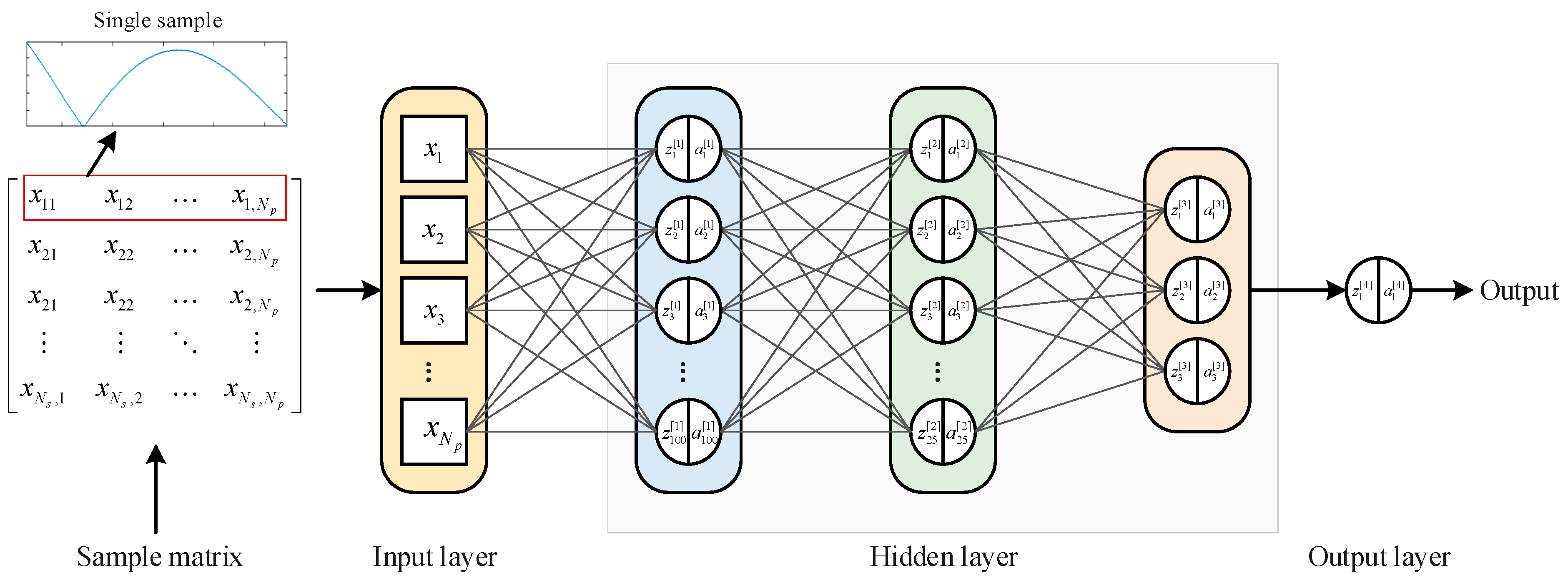
The simulation uses the back propagation (BP) neural network, which is set as a four-layer network model. The feature numbers of each layer are, respectively, 1000, 100, 25, and 3. The network structure is shown in the following figure (Figure 9).

The learning rate is set to 0.00001; the Adam optimizer and early-stopping is adopted; and the batch size is set to 32. With the increase in epoch number, the prediction accuracy of the train set and the test set is gradually improved, and the experimental results show that the accuracy tends to be stable when the number of iterations reaches 2000.

In the experiment, accuracy and cost are used to describe the training process of the neural network model. The accuracy denotes the prediction accuracy of the pre-trained model for the test set. The accuracy can be expressed as

$$Accuracy=\frac{T{P}_A+T{P}_B+T{P}_C}{N_{test}},$$

(17)

where $T{P}_A$, $T{P}_B$, and $T{P}_C$ denote the number of times that both the predicted result and the actual sample type are stripmap, scan, and spotlight, respectively; $N_{test}$ denotes the number of samples in the test set.

The cost is an important parameter that determines how well a machine learning model performs for a given train set. Generally, the smaller the function value, the better the model fits. The cost can be expressed as

$$Cost=-\frac{1}{N_{train}}{\displaystyle \sum _{i=1}^{N_{train}}\left[y^{(i)}\log {\widehat{y}}^{(i)}+\left(1-y^{(i)}\right)\log \left(1-{\widehat{y}}^{(i)}\right)\right]},$$

(18)

where $N_{test}$ denotes the number of samples in the train set; $y^{(i)},i=1,2,\dots ,N_{train}$ denotes the label value of the i-th sample; and ${\widehat{y}}^{(i)},i=1,2,\dots ,N_{train}$ denotes the value that the model classifier predicts for the i-th sample.

4.1. Effect of SNR on Identification Accuracy

SNR is the primary factor that affects the identification accuracy. The signal will be submerged in the noise when the noise power is too high compared with the SAR signal power. In this subsection, simulation experiments are conducted on the identification accuracy for different receiving SNRs. In the following experiments, SNR is defined as the ratio of the average SAR signal power to the average noise power during jammer sampling. The specific parameter-setting ranges for the test set are shown in the following table (

Table 3. Range of test set parameters.

Parameter	Value	Step-Size
Range antenna length	1 m~2 m	0.5 m
Azimuth antenna length	10 m~15 m	2.5 m
Carrier frequency	1.25 GHz~9.6 GHz	4.2 GHz
Bandwidth	10 MHz~30 MHz	10 MHz
Platform height	736 km~770 km	37.75 m
Elevation angle	12.5°~20°	7.5°
Squint angle	1°~3°	1°
Number of sub-swaths for scan SAR	4~6	2
Azimuth coordinates of jammer	2 km
Ground range coordinates of jammer	80 km
SNR	-8 dB~12 dB	4 dB

). Besides, the other parameters are kept the same as in the process of the train set production, and 108 samples are generated for each operating mode, respectively.

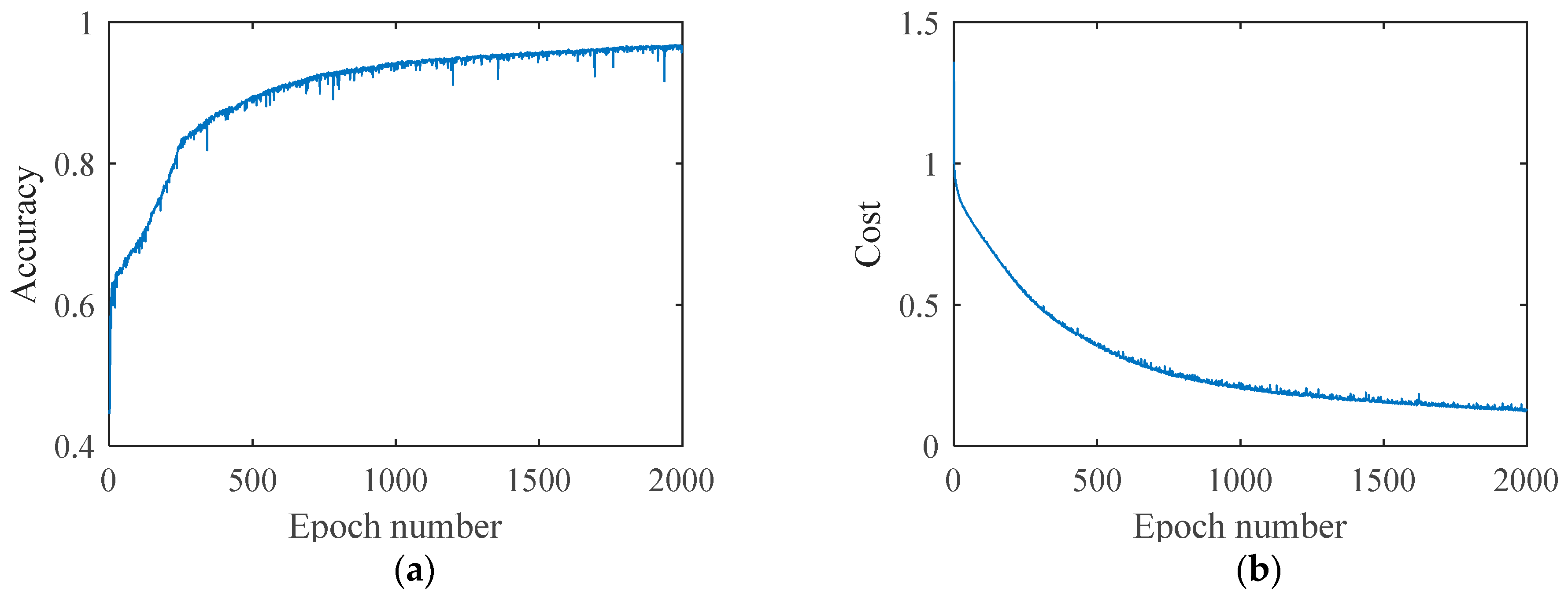
In the experiment, the train set containing 10,800 samples and the test set containing 324 samples were input into the network, where the train set and the test set have the same number of samples for stripmap, scan, and spotlight. When the number of the training epochs is set to 2000, the accuracy for the train set and the loss curve are shown in the figure below (Figure 10).

In the process of producing the test set, the SNR is set from −8 dB to 12 dB and the step-size is set to 4 dB. The prediction accuracy of the pre-trained network for each test set is shown in the table below (

Table 4. The prediction accuracy for different SNRs.

SNR	−8 dB	−4 dB	0 dB	4 dB	8 dB	12 dB
Accuracy (this method)	75.62%	80.86%	85.49%	87.04%	88.58%	88.89%

).

As shown in the table above, the average prediction accuracy rate can reach 85% when the SNR is set above 0 dB. However, the identification accuracy apparently decreases with the reduction of SNR, especially when the SNR is less than 0 dB.

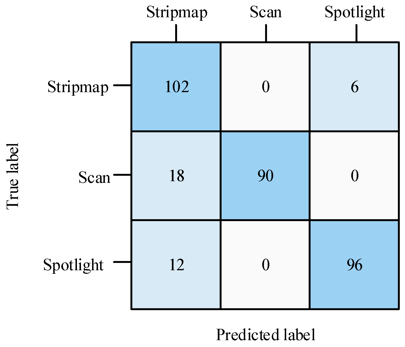
When the SNR is set to 12 dB, the classification confusion matrix of the method proposed in this paper is shown in the figure below (Figure 11).

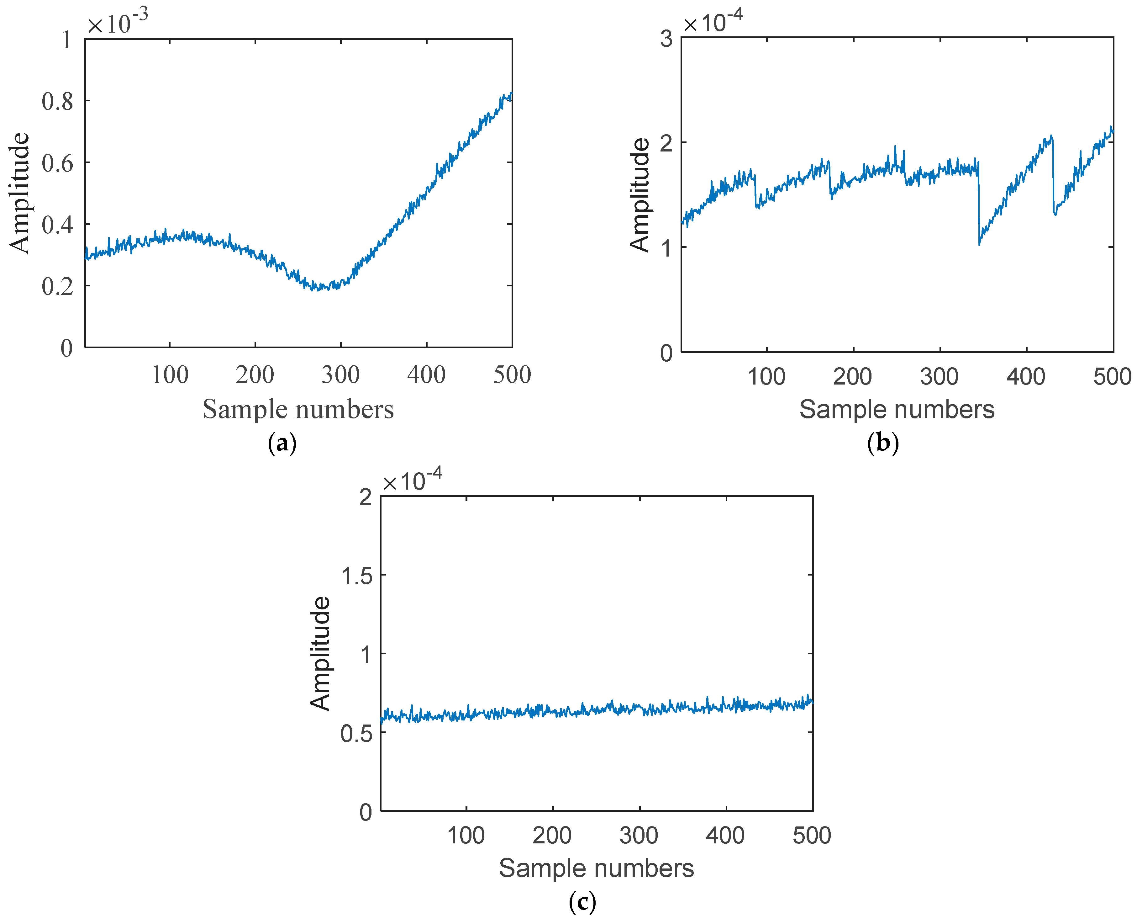
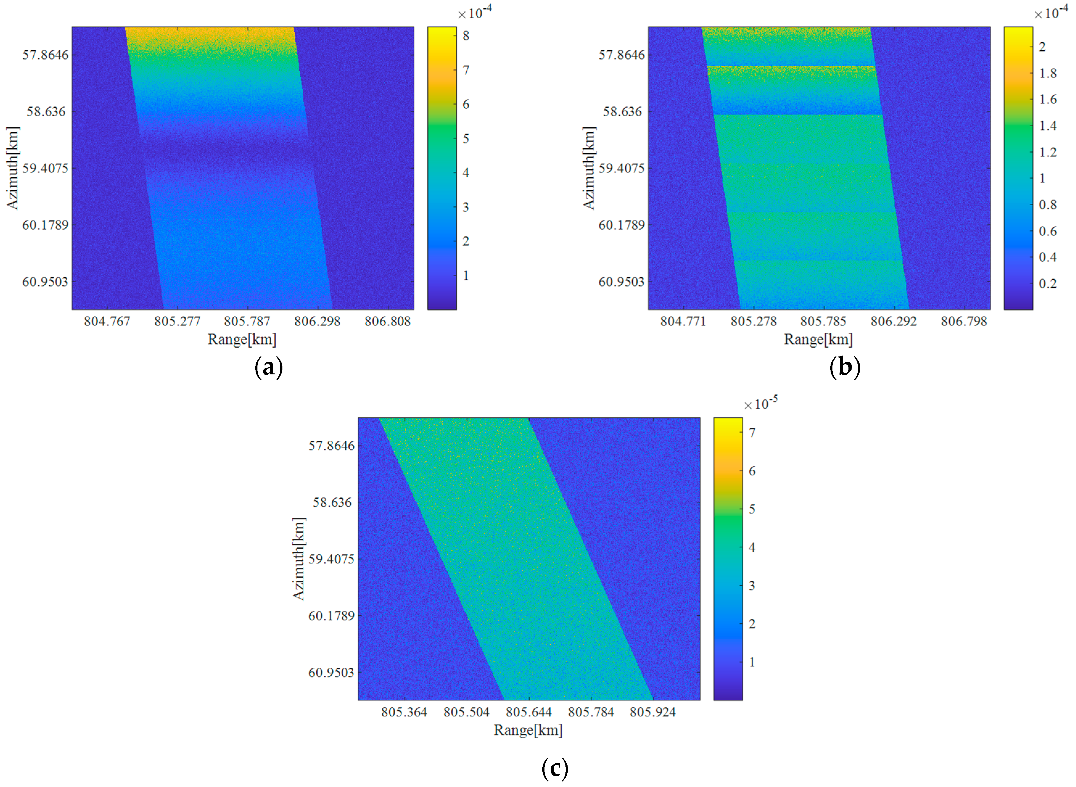
As shown in the above figure, stripmap samples are easier to identify than scan or spotlight samples. At the same time, scan and spotlight samples are more likely to be misidentified as stripmap samples. Two sample cases of misidentification are shown in the figure below (Figure 12). We found that when the signal power is too low, which is usually due to the intercepted signal being in the low-gain area of the antenna pattern, the difficulty of identification will be increased. In this regard, we can deploy several jammers at different locations (generally along the azimuth) to ensure that the intercepted signal power is high enough.

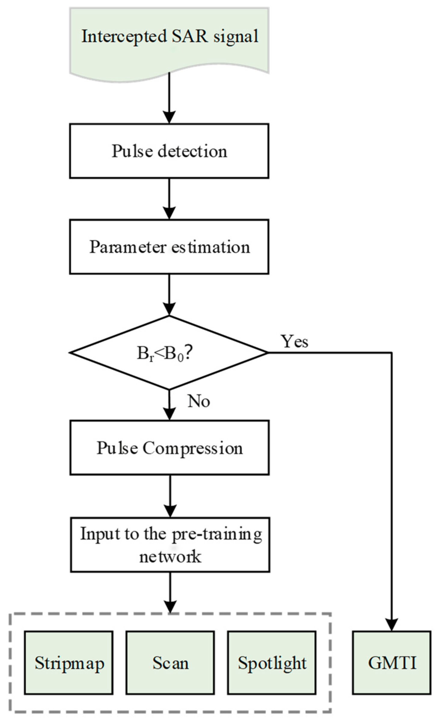
Since the proposed method is based on sidelobe reconnaissance, the signal experiences sidelobe decay. In order to compensate for the case of low SNR, we further consider using a matching filter to enhance the peak signal-to-noise ratio (PSNR), and the compressed signals are used to make a mode identification. To this end, the fractional Fourier transform (FrFT) algorithm is employed to obtain the required parameters. The detailed process to obtain the filter is as follows.

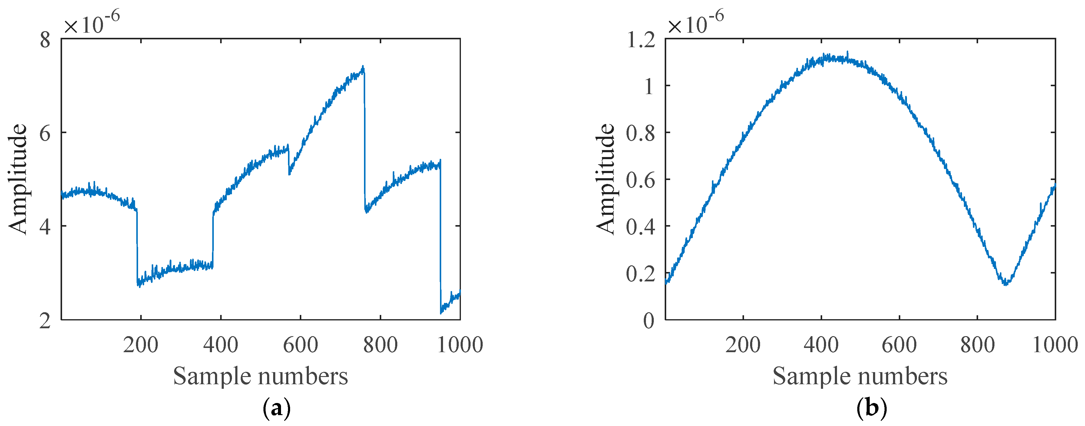
First, pulse detection is performed and then some intra-pulse parameters such as pulse duration and pulse repetition interval (PRI) can be estimated [43]. Then, we extract the first several pulses intercepted and estimate the frequency-modulated rate by the FrFT algorithm so that pulse compression can be performed.

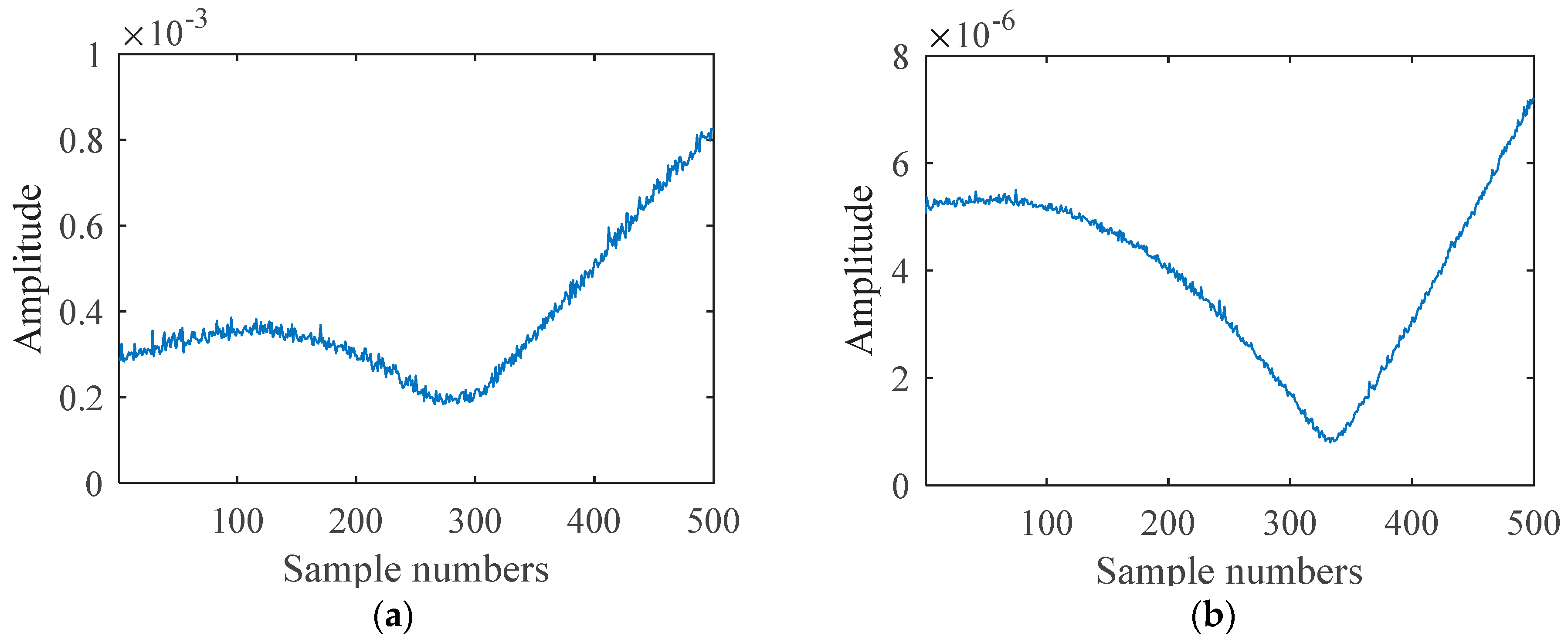
The amplitude of a section of intercepted signal before and after pulse compression is shown in the figure below (Figure 13).

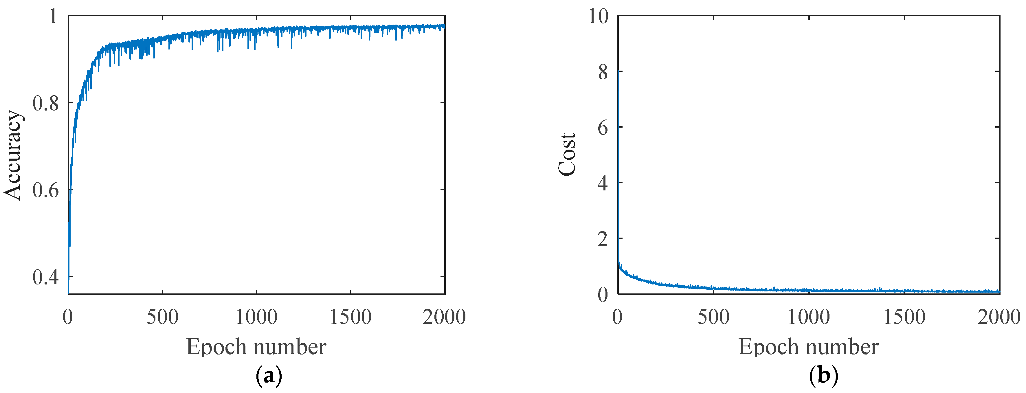
The data set with pulse compression is trained and predicted with other settings being unchanged. When the number of epochs is set to 2000, the accuracy for the train set and the loss curve are shown in the figure below (Figure 14).

Clearly, the network with pulse compression obtains an improved convergence rate which results from a higher SNR. In the process of producing the test set, the SNR is set from −8 dB to 12 dB and the step-size is set to 4 dB. The prediction accuracy of the pre-trained network with pulse compression as well as the method proposed in [32] for each test set is shown in the table below (

Table 5. The prediction accuracy with pulse compression for different SNRs.

SNR	−8 dB	−4 dB	0 dB	4 dB	8 dB	12 dB
Accuracy	89.81%	91.67%	91.67%	90.74%	90.43%	91.36%
Accuracy [32]	77.16%	82.10%	84.57%	86.73%	87.35%	88.58%

).

As shown in the table above, when the SNR is lower than 12 dB and higher than −8 dB, the identification accuracy rate remains at about 90% and will not deteriorate rapidly with the decrease in SNR. Therefore, the method based on the FrFT estimation algorithm can cope with the situation of poor SNR.

A Gated Recurrent Unit (GRU) neural network, an improved recurrent neural network, is employed in [32]. The experimental results show that the accuracy of the proposed method is slightly higher than the method employed in [32] when the SNR is higher than 0 dB; but, the accuracy of the method with pulse compression is much higher than the method employed in [32].

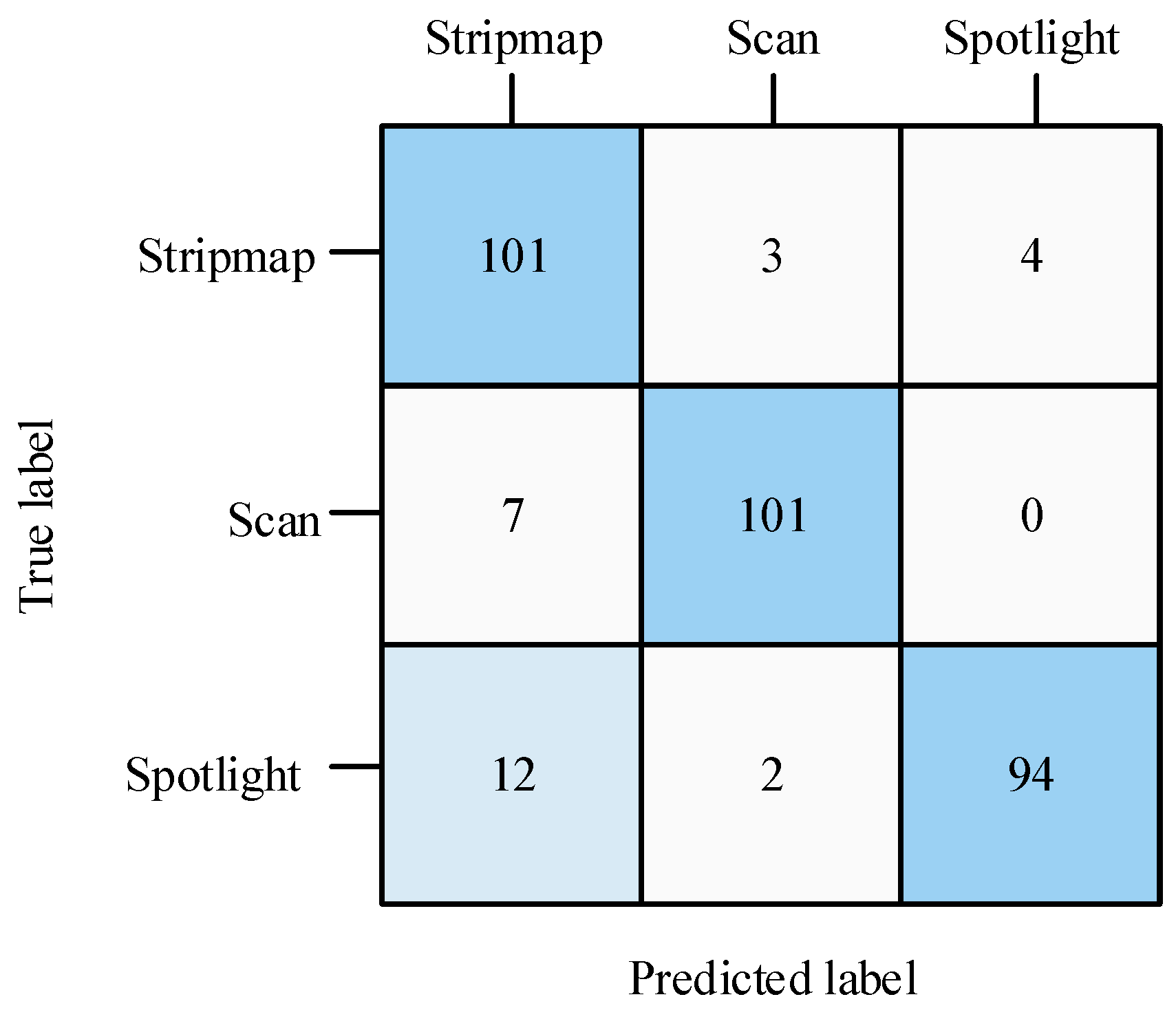
When the SNR is set to 12 dB, the classification confusion matrix of the method with pulse compression is shown in the figure below (Figure 15).

As shown in the above figure, compared with Figure 11, the identification accuracy has been improved. Similarly, scan and spotlight samples are more likely to be misidentified as stripmap samples.

4.2. Effect of the Jammer Position

Considering that the relative position of the jammer is unpredictable and uncontrollable when intercepting SAR signals, this subsection will verify the robustness of this method to the uncertainty of the relative position of the jammer.

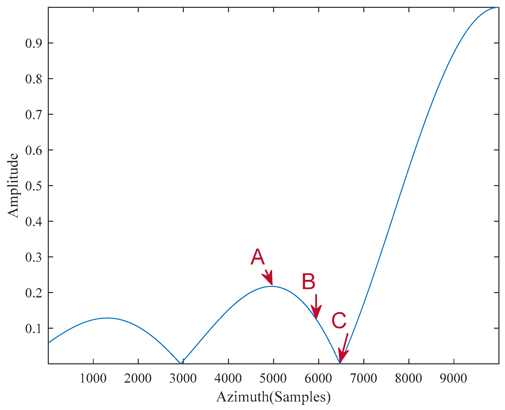
A part of the antenna pattern in azimuth for the point target is shown in the figure below (Figure 16). In the experiment, three typical jammer positions are selected along the azimuth as marked in the figure below (Figure 16). Specifically, among them, one is placed at the peak of the first sidelobe, one at the trough between the main lobe and the first sidelobe, and one at the midpoint between the former two.

Three jammers are placed at A, B, and C, respectively, as shown in the figure above, the SNR is set to 12 dB, and other settings are consistent with the experiment in Section 4.1. The training results are shown in the following table (

Table 6. The prediction accuracy when the jammer is set at points A, B, and C, respectively.

Without Pulse Compression		With Pulse Compression
Position	Accuracy	Position	Accuracy
A	91.05%	A	95.06%
B	89.51%	B	93.83%
C	86.73%	C	92.28%

).

Apparently, when the jammer is deployed at the above three typical positions, the identification accuracy rate can maintain itself above 86% and the rate can reach above 90% when pulse compression is employed. Hence, the robustness of this method to the jammer position is verified experimentally.

4.3. Effect of the Number of the Accumulated Pulses

The number of accumulated pulses required is closely related to the identification speed. As the number of accumulated pulses increases, the identification accuracy will increase, while the time required for identification will also increase. If an acceptable identification accuracy can be obtained with fewer pulses, the reconnaissance system for the SAR operating mode will be much more efficient. Therefore, this subsection discusses the relationship between the number of accumulated pulses and identification accuracy, so as to obtain an empirical optimal accumulated pulse number, which can provide a reference for future engineering application.

The following experiments set the number of the intercepted pulses from 100 to 1000, respectively, and the SNR is set to 12 dB while other experimental settings are consistent with Section 4.1. The experimental results are shown in the table below (

Table 7. Accuracy results for the different numbers of accumulated pulses.

Without Pulse Compression		With Pulse Compression
Np	Accuracy	Np 1	Accuracy
1000	88.89%	1000	91.36%
900	89.81%	900	87.35%
800	87.96%	800	88.89%
700	87.35%	700	88.27%
600	87.04%	600	90.12%
500	82.10%	500	87.96%
400	81.48%	400	87.65%
300	79.32%	300	81.79%
200	71.91%	200	78.09%
100	57.41%	100	63.58%

¹ ‘Np’ denotes the number of the accumulated pulses.

).

The experimental results show that without pulse compression, the identification accuracy will become less than 85% when the accumulated pulse number is reduced to 500. Furthermore, with the reduction of the accumulated pulse number, the accuracy will decrease sharply. With pulse compression employed, the accuracy can still remain above 85% when the pulse number is reduced to 400.

In order to balance the identification accuracy and the speed, it is appropriate to set the accumulated pulse number to 600 without pulse compression. Besides, the number can be set to 400 with pulse compression employed.

5. Conclusions

To solve the problem of SAR operating mode identification, an intelligent model based on sidelobe reconnaissance and machine learning is proposed in this paper. This method uses the SAR signal intercepted by the ground-based jammer as the input and can identify four operating modes (stripmap, scan, spotlight, and GMTI). The method takes account of both identification accuracy and speed, and it has good robustness to low SNR and uncertainty of the jammer’s position. Furthermore, pulse compression can be employed to improve the robustness to low SNR. Finally, the experimental results show that the method can maintain satisfactory performance even if the accumulated pulse number is reduced to 400 when pulse compression is employed. In the future, in order to cope with complex electromagnetic environments and the development of radar technologies, we will further discuss some better machine learning algorithms to improve the employed model in this paper.

References

1. Cheney, M. A mathematical tutorial on synthetic aperture radar. SIAM Rev. 2001, 43, 301–312. [Google Scholar] [CrossRef]
2. Deng, Y.; Yu, W.; Zhang, H.; Wang, W.; Liu, D.; Wang, R. Forthcoming Spaceborne SAR Development. J. Radars 2020, 9, 1–33. [Google Scholar]
3. Moreira, A.; Prats-Iraola, P.; Younis, M.; Krieger, G.; Hajnsek, I.; Papathanassiou, K.P. A tutorial on synthetic aperture radar. IEEE Geosci. Remote Sens. Mag. 2013, 1, 6–43. [Google Scholar] [CrossRef]
4. Ouchi, K. Recent Trend and Advance of Synthetic Aperture Radar with Selected Topics. Remote Sens. 2013, 5, 716–807. [Google Scholar] [CrossRef]
5. Jin, G.; Wang, Y.; Zhu, D.; Niu, S.; Yan, H. A Reconfigurable MIMO-SAR Transmission Scheme Based on Inter-Pulse and Intra-Pulse Joint Phase Modulation. IEEE Trans. Signal Process. 2022, 70, 4265–4276. [Google Scholar] [CrossRef]
6. Gan, R.-b.; Wang, J.-g. Improvement of the responsive deception for spaceborne SAR. J. Univ. Electron. Sci. Technol. China 2005, 34, 614–617. [Google Scholar]
7. Liu, Y.; Wang, W.; Pan, X.; Xu, L.; Wang, G. Influence of Estimate Error of Radar Kinematic Parameter on Deceptive Jamming Against SAR. IEEE Sens. J. 2016, 16, 5904–5911. [Google Scholar] [CrossRef]
8. Paine, A.S. An adaptive beamforming technique for countering synthetic aperture radar (SAR) jamming threats. In Proceedings of the 2007 IEEE Radar Conference, Waltham, MA, USA, 17–20 April 2007; pp. 630–634. [Google Scholar]
9. Sun, Q.; Shu, T.; Thou, S.; Tang, B.; Yu, W. A Novel Jamming Signal Generation Method for Deceptive SAR Jammer. In Proceedings of the 2014 IEEE Radar Conference, Rome, Italy, 8–10 October 2014; pp. 1174–1178. [Google Scholar]
10. Sun, Q.; Shu, T.; Yu, K.-B.; Yu, W. Efficient Deceptive Jamming Method of Static and Moving Targets Against SAR. IEEE Sens. J. 2018, 18, 3610–3618. [Google Scholar] [CrossRef]
11. Cheng, Y.; Zhu, D.; Jin, G.; Zhang, J.; Niu, S.; Wang, Y. A Novel Intrapulse Repeater Mainlobe-Jamming Suppression Method with MIMO-SAR. IEEE Geosci. Remote Sens. Lett. 2022, 19, 4507805. [Google Scholar] [CrossRef]
12. Wang, Y.; Jin, G.; Song, C.; Lu, P.; Han, S.; Lv, J.; Zhang, Y.; Wu, D.; Zhu, D. Parameterized and Large-dynamic-range Two-dimensional Precise Controllable SAR Jamming: Characterization, Modeling, and Analysis. IEEE Trans. Geosci. Remote Sens. 2023, 61, 5209416. [Google Scholar]
13. Huang, B.; Wang, W.-Q.; Zhang, S.; Wang, H.; Gui, R.; Lu, Z. A Novel Approach for Spaceborne SAR Scattered-Wave Deception Jamming Using Frequency Diverse Array. IEEE Geosci. Remote Sens. Lett. 2020, 17, 1568–1572. [Google Scholar] [CrossRef]
14. Sun, Q.; Shu, T.; Yu, K.-B.; Yu, W. A Novel Deceptive Jamming Method Against Two-Channel SAR-GMTI Based on Two Jammers. IEEE Sens. J. 2019, 19, 5600–5610. [Google Scholar] [CrossRef]
15. Zhao, B.; Huang, L.; Zhou, F.; Zhang, J. Performance Improvement of Deception Jamming Against SAR Based on Minimum Condition Number. IEEE J. Sel. Top. Appl. Earth Obs. Remote Sens. 2017, 10, 1039–1055. [Google Scholar] [CrossRef]
16. Zhao, B.; Zhou, F.; Bao, Z. Deception Jamming for Squint SAR Based on Multiple Receivers. IEEE J. Sel. Top. Appl. Earth Obs. Remote Sens. 2015, 8, 3988–3998. [Google Scholar] [CrossRef]
17. HanYan, L.I.U.; HongJun, S.; ZengJu, C. Comparative study on stripmap mode, spotlight mode, and sliding spotlight mode. J. Grad. Sch. Acad. Sci. 2011, 28, 410–417. [Google Scholar]
18. Bin, D.; Yuliang, Q.; Yanpeng, L.; Hongqiang, W.; Xiang, L. Fast simulation of raw signals from natural scenes for squint stripmap SAR. In Proceedings of the 2009 2nd Asian-Pacific Conference on Synthetic Aperture Radar (APSAR 2009), Xi’an, China, 26–30 October 2009; pp. 235–238. [Google Scholar]
19. Chen, J.; Wang, K.; Yang, W.; Liu, W. Accurate Reconstruction and Suppression for Azimuth Ambiguities in Spaceborne Stripmap SAR Images. IEEE Geosci. Remote Sens. Lett. 2017, 14, 102–106. [Google Scholar] [CrossRef]
20. Dogan, O.; Kartal, M. Efficient Stripmap-Mode SAR Raw Data Simulation Including Platform Angular Deviations. IEEE Geosci. Remote Sens. Lett. 2011, 8, 784–788. [Google Scholar] [CrossRef]
21. Mao, X.H.; Zhu, D.Y.; Zhu, Z.D. Signatures of Moving Target in Polar Format Spotlight SAR Image. Prog. Electromagn. Res. 2009, 92, 47–64. [Google Scholar] [CrossRef]
22. Mittermayer, J.; Lord, R.; Bömer, E. Sliding spotlight SAR processing for TerraSAR-X using a new fon-nulation of the extended chirp scaling algorithm. In Proceedings: Learning from Earth’s Shapes And Sizes, Proceedings of the IGARSS 2003: IEEE International Geoscience and Remote Sensing Symposium; IEEE: New York, NY, USA, 2003; Volumes I–VII, pp. 1462–1464. [Google Scholar]
23. Mittermayer, J.; Moreira, A.; Loffeld, O. Spotlight SAR data processing using the frequency scaling algorithm. IEEE Trans. Geosci. Remote Sens. 1999, 37, 2198–2214. [Google Scholar] [CrossRef]
24. Zhu, D.; Ye, S.; Zhu, Z. Polar Format Algorithm using Chirp Scaling for Spotlight SAR Image Formation. IEEE Trans. Aerosp. Electron. Syst. 2008, 44, 1433–1448. [Google Scholar] [CrossRef]
25. Bamler, R.; Eineder, M. ScanSAR processing using standard high precision SAR algorithms. IEEE Trans. Geosci. Remote Sens. 1996, 34, 212–218. [Google Scholar] [CrossRef]
26. Holzner, J.; Bamler, R. Burst-mode and ScanSAR interferometry. IEEE Trans. Geosci. Remote Sens. 2002, 40, 1917–1934. [Google Scholar] [CrossRef]
27. Jin, M.Y. Optimal range and Doppler centroid estimation for a ScanSAR system. IEEE Trans. Geosci. Remote Sens. 1996, 34, 479–488. [Google Scholar] [CrossRef]
28. Li, N.; Wang, R.; Deng, Y.; Chen, J.; Zhang, Z.; Liu, Y.; Xu, Z.; Zhao, F. Improved Full-Aperture ScanSAR Imaging Algorithm Based on Aperture Interpolation. IEEE Geosci. Remote Sens. Lett. 2015, 12, 1101–1105. [Google Scholar] [CrossRef]
29. Chen, Y.; Wu, Y.; Jia, X. Surveillance study of spaceborne synthetic aperture radar in different working modes. Comput. Eng. Appl. 2013, 49, 223–227. [Google Scholar]
30. Tang, X.; Li, C.; Sun, B. Inversion method of spaceborne SAR operating mode based on genetic algorithm. Space Electron. Technol. 2013, 10, 90–94. [Google Scholar]
31. Xia, Z.; Zhong, H.; Chen, W. Identification of spaceborne SAR operating mode in reconnaissance mode. J. Hangzhou Dianzi Univ. (Nat. Sci.) 2017, 37, 36–40. [Google Scholar] [CrossRef]
32. He, J.; Zhang, Y.-S.; Yin, C.-B. Operating modes identification of spaceborne SAR based on deep learning. J. Zhejiang Univ. (Eng. Sci.) 2022, 56, 1676–1684. [Google Scholar]
33. Ioffe, S.; Szegedy, C. Batch Normalization: Accelerating Deep Network Training by Reducing Internal Covariate Shift. In Proceedings of the International Conference on Machine Learning, Lille, France, 6–11 July 2015; Volume 37, pp. 448–456. [Google Scholar]
34. Olkhovskiy, M.; Mullerova, E.; Martinek, P. Impulse signals classification using one dimensional convolutional neural network. J. Electr. Eng.-Elektrotechnicky Cas. 2020, 71, 397–405. [Google Scholar] [CrossRef]
35. Qu, W.; Wu, Y.; Jia, X. Study on SAR Antenna Side Lobe Reconnaissance. J. Acad. Equip. Command. Technol. 2004, 15, 103–107. [Google Scholar]
36. Bachmann, M.; Schwerdt, M.; Braeutigam, B. Accurate Antenna Pattern Modeling for Phased Array Antennas in SAR Applications-Demonstration on TerraSAR-X. Int. J. Antennas Propag. 2009, 2009, 492505. [Google Scholar] [CrossRef]
37. Kim, S.Y.; Sung, J.B.; Torre, A. In-Orbit Antenna Pattern Extraction Method for Active Phased-Array SAR Antennas. IEEE Antennas Wirel. Propag. Lett. 2016, 15, 317–320. [Google Scholar] [CrossRef]
38. Shimada, M.; Freeman, A. A Technique for Measurement of Spaceborne Sar Antenna Patterns Using Distributed Targets. IEEE Trans. Geosci. Remote Sens. 1995, 33, 100–114. [Google Scholar] [CrossRef]
39. Candan, Ç.; Kutay, M.A.; Ozaktas, H.M. The discrete fractional Fourier transform. IEEE Trans. Signal Process. 2000, 48, 1329–1337. [Google Scholar] [CrossRef]
40. Ozaktas, H.M.; Ankan, O.; Kutay, M.A.; Bozdagi, G. Digital computation of the fractional Fourier transform. IEEE Trans. Signal Process. 1996, 44, 2141–2150. [Google Scholar] [CrossRef]
41. Pei, S.C.; Yeh, M.H.; Tseng, C.C. Discrete fractional Fourier transform based on orthogonal projections. IEEE Trans. Signal Process. 1999, 47, 1335–1348. [Google Scholar] [CrossRef]
42. Xinghao, Z.; Ran, T.; Bing, D. Practical Normalization methods in the digital computation of the fractional Fourier transform. In Proceedings of the 2004 7th International Conference on Signal Processing Proceedings, Beijing, China, 31 August–4 September 2004; Volumes 1–3, pp. 105–108. [Google Scholar]
43. Wang, Y. Research on the Modulation Recognition Algorithms and Parameter Estimation Algorithms of Radar Signal. Master’s Thesis, National University of Defense Technology, Changsha, China, 2012. [Google Scholar]
Figure 1. Illustration of different SAR operating modes, where ‘SSW’ is the abbreviation for sub-swath. (a) Stripmap SAR; (b) scan SAR; (c) spotlight SAR.
Remotesensing 16 01234 g001
Figure 2. Geometric relationship of stripmap SAR, where η = η c denotes the beam center crossing time.
Remotesensing 16 01234 g002
Figure 3. Geometric relationship of scan SAR, where SSW is the abbreviation for sub-swath.
Remotesensing 16 01234 g003
Figure 4. Geometric relationship of spotlight SAR.
Remotesensing 16 01234 g004
Figure 5. Amplitude of the intercepted signal of each mode (unit: Volt, SNR: 0 dB). (a) Stripmap SAR; (b) scan SAR; (c) spotlight SAR.
Remotesensing 16 01234 g005
Figure 6. Samples of each mode. (a) Stripmap SAR; (b) scan SAR; (c) spotlight SAR.
Remotesensing 16 01234 g006
Figure 7. A sample example in difficult cases. (a) A sample of stripmap SAR; (b) a sample of spotlight SAR.
Remotesensing 16 01234 g007
Figure 8. The workflow of the proposed SAR operating mode identification method.
Remotesensing 16 01234 g008
Figure 9. The structure of the BP neural network, where ‘Ns’ denotes the number of the samples and ‘Np’ denotes the number of the accumulated pulses per sample.
Remotesensing 16 01234 g009
Figure 10. Curve diagram of training accuracy and loss. (a) Training accuracy curve; (b) training loss curve.
Remotesensing 16 01234 g010
Figure 11. Classification confusion matrix of the method proposed in this paper.
Remotesensing 16 01234 g011
Figure 12. Sample cases of misidentification. (a) Scan sample; (b) spotlight sample.
Remotesensing 16 01234 g012
Figure 13. The amplitude of the signal before and after pulse compression. (a) Before pulse compression; (b) after pulse compression.
Remotesensing 16 01234 g013
Figure 14. Curve diagram of training accuracy and loss. (a) Training accuracy curve; (b) training loss curve.
Remotesensing 16 01234 g014
Figure 15. Classification confusion matrix of the method with pulse compression.
Remotesensing 16 01234 g015
Figure 16. The antenna pattern in the azimuth plane for the point target.
Remotesensing 16 01234 g016