Article

Feasibility of Urban–Rural Temperature Difference Method in Surface Urban Heat Island Analysis under Non-Uniform Rural Landcover: A Case Study in 34 Major Urban Agglomerations in China

1
State Key Laboratory of Efficient Utilization of Arid and Semi-Arid Arable Land in Northern China, Institute of Agricultural Resources and Regional Planning, Chinese Academy of Agricultural Sciences, Beijing 100081, China
2
Academy of Agricultural Planning and Engineering, Beijing 100125, China
3
ICube Laboratory, UMR 7357, CNRS-University of Strasbourg, 300 bd S’ebastien Brant, CS 10413, F-67412 Illkirch Cedex, France
4
Faculty of Land Resource Engineering, Kunming University of Science and Technology, Kunming 650093, China
5
State Key Laboratory of Resources and Environment Information System, Institute of Geographic Sciences and Natural Resources Research, Chinese Academy of Sciences, Beijing 100101, China
*
Author to whom correspondence should be addressed.
Remote Sens. 2024, 16(7), 1232; https://doi.org/10.3390/rs16071232
Submission received: 5 March 2024 / Revised: 26 March 2024 / Accepted: 30 March 2024 / Published: 31 March 2024

Abstract

:
The urban–rural temperature difference is widely used in measuring surface urban heat island intensity (SUHII), where the accurate determination of rural background is crucial. However, traditionally, the entire permeable rural surface has been selected to represent the background temperature, leaving uncertainty about the impact of non-uniform rural surfaces with multiple land covers on the accuracy of SUHII quantification. In this study, we proposed two quantifications of SUHII derived from the primary (SUHII1) and secondary (SUHII2) land types, respectively, which successively occupy over 40–50% of whole rural regions. The spatial integration and temporal variation of SUHII1 and SUHII2 were compared with the result from whole rural regions (SUHII) within 34 urban agglomerations (UAs) in China. The results showed that the SUHII1 and SUHII2 differed slightly with SUHII, and the correlation coefficients of SUHII and SUHII1/SUHII2 are generally above 0.9 in most (32) UAs. Regarding the long-term SUHII between 2003 and 2019, the three methods demonstrated similar seasonal patterns, although SUHII1 (or SUHII2) tended to overestimate or underestimate compared to SUHII. As for the multi-year integration at the regional scale, the day–night cycle and monthly variations of SUHII1 and SUHII were found to be identical for each geographical division separately, indicating that the spatiotemporal pattern revealed by SUHII is minimally affected by the diversity of rural landcover types. The findings confirmed the viability of the urban–rural LST difference method for measuring long-term regional SUHII patterns under non-uniform rural land cover types.

1. Introduction

In recent years, the phenomenon of the surface urban heat island (SUHI) has been observed in thousands of cities globally [1,2]. Numerous studies have indicated that the SUHI contributed to various environmental changes, including alterations in regional climate [3], compromised vegetation growth [4], and degradation of water and air quality [5]. Given that urban areas accommodate approximately 55% of the world’s population, these changes pose threats to human well-being and development [6], leading to increased morbidity and mortality rates [7], and even potential risks of violence [8]. As urbanization profoundly impacts human living conditions [9], accurate monitoring of SUHI patterns is essential to support effective strategies for managing the urban thermal environment.
Advancements in remote sensing technology have facilitated the revelation of spatiotemporal patterns of global SUHIs and their associated driving factors on various scales using land surface temperature (LST) products [10,11,12]. Currently, the urban–rural difference method stands as one of the most prevalent approaches for quantifying SUHI intensity (SUHII). However, the identification of urban and rural regions varies among different studies conducted in diverse global cities [13,14,15,16]. As the accuracy of SUHII is pivotal for depicting its spatial and temporal patterns [1,17], it is imperative to investigate the sensitivity of SUHII analysis to different quantification indices.
Accurate delineation of rural regions is crucial for obtaining background LST during SUHII calculation. Traditionally, the process of SUHII quantification first used land use/land cover (LULC) data to identify the urban and rural areas [18]. After identifying the urban clusters, a buffer at a fixed distance from the urban center or an area with a fixed multiple of the urban area is generally defined as its rural region. Generally, urban and rural were identified by differentiating the continuous urban regions from rural pixels enclosed in fixed urban administrative boundaries [13,19] or in a dynamic form of varied urban regions with urban expansion and buffered rural regions [20]. It is convenient and feasible to provide reliable results for global SUHI. However, analysis based on the LST of entire rural land surfaces and woodlands, respectively, demonstrated contrasting SUHII patterns in a semi-arid city [21]. Currently, methods prioritize elevation control and water body exclusion [2,19], while the impact of the diversity of rural land cover types on regional SUHI studies involving multiple cities has received limited attention [22]. It has been stressed that the proximity to water bodies in urban and non-urban areas should be similar, and the altitudinal difference between urban and non-urban points should be as small as possible [23]; yet, whether the selection of different rural components dominates the regional pattern of SUHII is unexplored. For rural surfaces comprising various non-uniform land covers, it remains unclear whether SUHII quantification based on the entire background affects its multi-scale spatiotemporal patterns [10]. Therefore, to accurately depict the evolution of SUHII and its driving factors, it is crucial to verify the feasibility of SUHII quantification under diverse rural land cover types [24].
As China undergoes rapid urbanization, it has emerged as one of the most populous developing countries with vast terrain, complex climate and topography, and diverse rural land cover types corresponding to cities in different regions [25,26]. Numerous studies have revealed the presence of SUHI phenomena in most large cities across China, elucidating them at multiple scales [13,27,28]. Urbanization has significantly contributed to local and regional surface warming [29]. Recent studies have shown the magnitude of SUHII in China’s major cities to be definition-independent [2,13], yet their diurnal and seasonal patterns conflict across these definitions [30]. Considering the sensitivity of SUHII to rural backgrounds with compound land cover types in China, it is necessary to fully compare different quantifications of SUHII in investigating its regional patterns.
Hence, this study first reveals rural land cover types and urban expansion in 34 of China’s major urban agglomerations (UAs) between 2003 and 2019. Subsequently, new quantifications of SUHII are proposed based on the principal and secondary rural land cover components. To verify the feasibility and credibility of the urban–rural difference method in depicting patterns and temporal variations of regional SUHII, SUHII from different quantification methods are compared within each geographical division. Finally, the spatiotemporal pattern of SUHII in China, including the day–night cycle, monthly variation, and interannual trend, is further investigated to support the feasibility of SUHII quantified by the entire rural region.

2. Materials and Methods
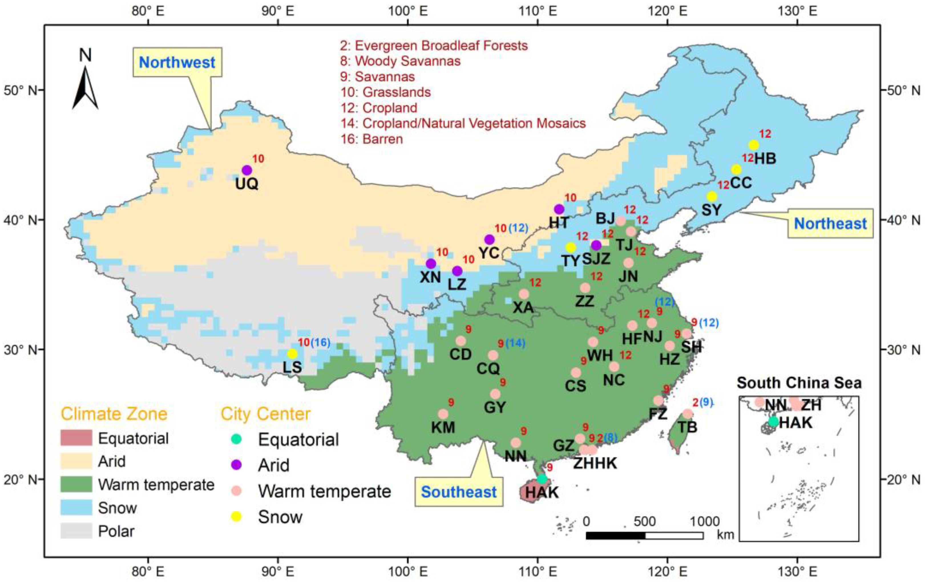
2.1. Study Area

In China, the main population is concentrated in provincial-level administrative regions, which are economically developed, experiencing rapid urban development, and have been widely concerned with urban environment issues in recent years. The study encompasses 34 of China’s provincial capitals, municipalities, and special administrative regions, chosen due to observed escalating trends in SUHI in recent years [31]. The primary and secondary rural regions, respectively, constituting approximately 40–50% of the total rural land use types for each city, were identified based on previous research [20] using land use data from MCD12Q1 between 2003 and 2019. Generally, China’s main cities can be grouped into six regions according to geographic variations regarding geographical location, climatic conditions, and economic development levels. While considering the similarity of rural land cover types and SUHII patterns [32], six major regions of China have been consolidated into three: Northwest, Northeast, and Southeast regions. The boundaries of these regions are delineated by interconnected provincial borders.
As shown in Figure 1, the center point is identified with the abbreviation of the city name (BJ: Beijing, CC: Changchun, CD: Chengdu, CQ: Chongqing, CS: Changsha, FZ: Fuzhou, GY: Guiyang, GZ: Guangzhou, HAK: Haikou, HB: Harbin, HF: Hefei, HK: Hong Kong, HT: Hohhot, HZ: Hangzhou, JN: Jinan, KM: Kunming, LS: Lhasa, LZ: Lanzhou, NC: Nanchang, NJ: Nanjing, NN: Nanning, SH: Shanghai, SJZ: Shijiazhuang, SY: Shenyang, TJ: Tianjin, TY: Taiyuan, UQ: Urumqi, WH: Wuhan, XA: Xi’an, XN: Xining, YC: Yinchuan, ZH: Zhuhai, ZZ: Zhengzhou); the principal and/or secondary landcover types in rural areas are marked with corresponding numbers. It should be noted that the urban area of Macau was connected with Zhuhai after executing the urban identification method (details in Section 2.3). The 34 cities are distributed with diverse rural landcover types, which were geographically divided into the Northwest, the Northeast, and the Southeast regions.
In the Northwest, characterized by an arid climate, grasslands dominate as the principal rural land cover. Notably, Yinchuan and Lhasa feature cropland and barren land as their secondary rural land types, respectively. The Southeast, predominantly in the warm temperate zone, comprises savannas and evergreen broadleaf forests as the primary rural land cover types. Notable variations include mixed land covers of savanna and cropland in Nanjing, Shanghai, and Chongqing, and combinations of evergreen broadleaf forests with woody savannas in Hong Kong. Conversely, Taipei features evergreen broadleaf forests and savannas. In the Northeast, cropland predominates as the principal rural land cover type. Concerning the Northeast region, the principal rural land type for each UA is cropland. The diverse rural land cover types across the 34 major UAs in China provide a suitable basis for analyzing the urban-rural LST difference method under complex, non-uniform rural backgrounds.

2.2. Data

2.2.1. MODIS Land Surface Temperature

The MODIS LST, widely employed in SUHII quantification [33,34,35], was sourced from the MOD11A1 and MYD11A1 datasets (Version 6) onboard the Terra and Aqua satellites. These datasets offer daily surface temperature/emissivity product data for each pixel, with a spatial resolution of 1 km and a sinusoidal projection. The transit times of the Terra and Aqua satellites are approximately 10:30 and 22:30 at local solar time, and 01:30 and 13:30 at local solar time, respectively. The period of available datasets is from 24 February 2000 to the present for MOD11A1 and from 4 July 2002 to the present for MYD11A1. For this study, all available global day/night LST datasets from 1 January 2003 to 31 December 2019 were utilized.

2.2.2. MODIS Land Cover Type

Annual land cover types were extracted from the MODIS Land Cover Type product (MCD12Q1, Version 6), providing global land cover distribution at annual intervals. This product utilizes supervised decision tree classification technology with MODIS Terra/Aqua reflectance data, offering a spatial resolution of 500 m. To align with the LST dataset timeframe, MCD12Q1 data from 2003 to 2019 were selected to obtain land use and land cover (LULC) types. The dataset comprises 17 land cover categories based on the International Geosphere-Biosphere Programme (IGBP) classification scheme [36] as detailed in Table 1. The Land Cover Type data were used to identify the primary and secondary rural land cover types.

2.2.3. Elevation

Surface elevation data were extracted from the GTOPO30 dataset with a spatial resolution of 1 km from the US Geological Survey (USGS, Reston, VA, USA). The center point for the digital elevation model (DEM) is given every 30 s of latitude and longitude worldwide. The latitude and longitude grid composed of these discrete points divides the earth’s surface into many quadrilateral grid areas so that the elevation value of any point in the grid area can be obtained by interpolation from the surrounding four grid points.

2.3. Quantification of SUHII

As the 34 UAs in China contain one or two main rural land types (Figure 1), the principal and secondary land types, respectively, refer to the components that successively occupy over 40–50% of whole rural regions. In this study, we compared the results of SUHIIs defined by different rural regions.
The urban extent that varied annually was identified using the city clustering algorithm (CCA) [37] with the LULC dataset. The city center was determined by the World Population Prospect (WUP) issued by the United Nations, and then based on the interconnection of urban regions, the urban clusters could be identified by an iterative search. The corresponding dynamic rural regions were identified as the equal-area buffer from the dynamic urban extents. Thereafter, both the whole rural region and the primary and secondary rural regions varied by year. SUHII was calculated in Equation (1) as the difference between urban and rural LST, excluding rural pixels with elevations exceeding ±200 m of the regional average based on the Dynamic Urban Extent method (DUE) [20]. Unlike DUE, which determines the average LST across the entire rural surface, rural LST pixels for pure primary and secondary rural surface components were selected to calculate corresponding reference LST. Equations (2) and (3) represent the new quantifications of SUHII, where average urban LST is subtracted by the average LST of the principal and secondary rural land cover types, respectively, yielding the corresponding SUHI intensity (SUHII1 and SUHII2). Subsequently, daytime and nighttime mean SUHIIs were averaged from Terra/Aqua results (approximately 10:30/13:30 and 01:30/22:30), and monthly and yearly mean SUHIIs were integrated from daily results. The new quantifications of SUHII1 and SUHII2 are shown in Equations (1) and (2) as follows:
SUHII = Tu − Tr,
SUHII1 = Tu − Tr1,
SUHII2 = Tu − Tr2,
where the Tu is the average urban LST, the Tr, Tr1 and Tr2 are the average LST of the whole, the principal and secondary rural land use types, respectively, and SUHII, SUHII1 and SUHII2 are the corresponding intensity of SUHI. Correspondingly, the SUHIs from the whole rural region were calculated in similar steps. Afterward, the daytime and nighttime mean SUHIIs were averaged by the result from Terra and Aqua. The monthly and yearly mean SUHIIs were integrated from the daily results.

3. Results

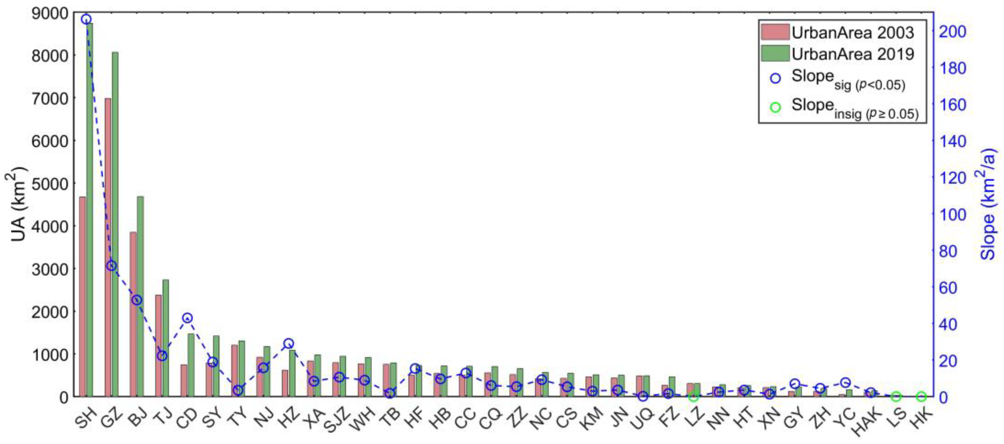
3.1. Urban Form Expansion

The urban form expansion of the 34 UAs identified by the CCA algorithm [37] is illustrated in Figure 2. The red and blue areas represent urban boundaries in 2003 and 2019, respectively. Notably, the urban areas identified by the CCA algorithm may surpass actual administrative boundaries, potentially connecting large cities with surrounding satellite cities. For instance, Shanghai and Guangzhou form urban agglomerations connecting the central large city with surrounding areas.
Figure 3 displays the urban area and change rate of each UA from 2003 to 2019. The changing rate was calculated using the Sen’s Slope. Notably, urban areas of Shanghai, Guangzhou, Beijing, and Tianjin exceed 2000 km2. Except for Lanzhou, Lhasa, and Hong Kong, all UAs exhibit a significant increasing trend in urban areas, with larger cities generally experiencing higher rates of change. For example, Shanghai, Guangzhou, Beijing, and Chengdu witness urban area expansions at rates exceeding 50 km2 per year. The expansion of urban form and size is typically accompanied by changes in surrounding rural land use types, emphasizing the necessity of employing dynamic urban-extent methods to accurately quantify SUHI intensity.

3.2. Comparison of Different SUHII Quantifications

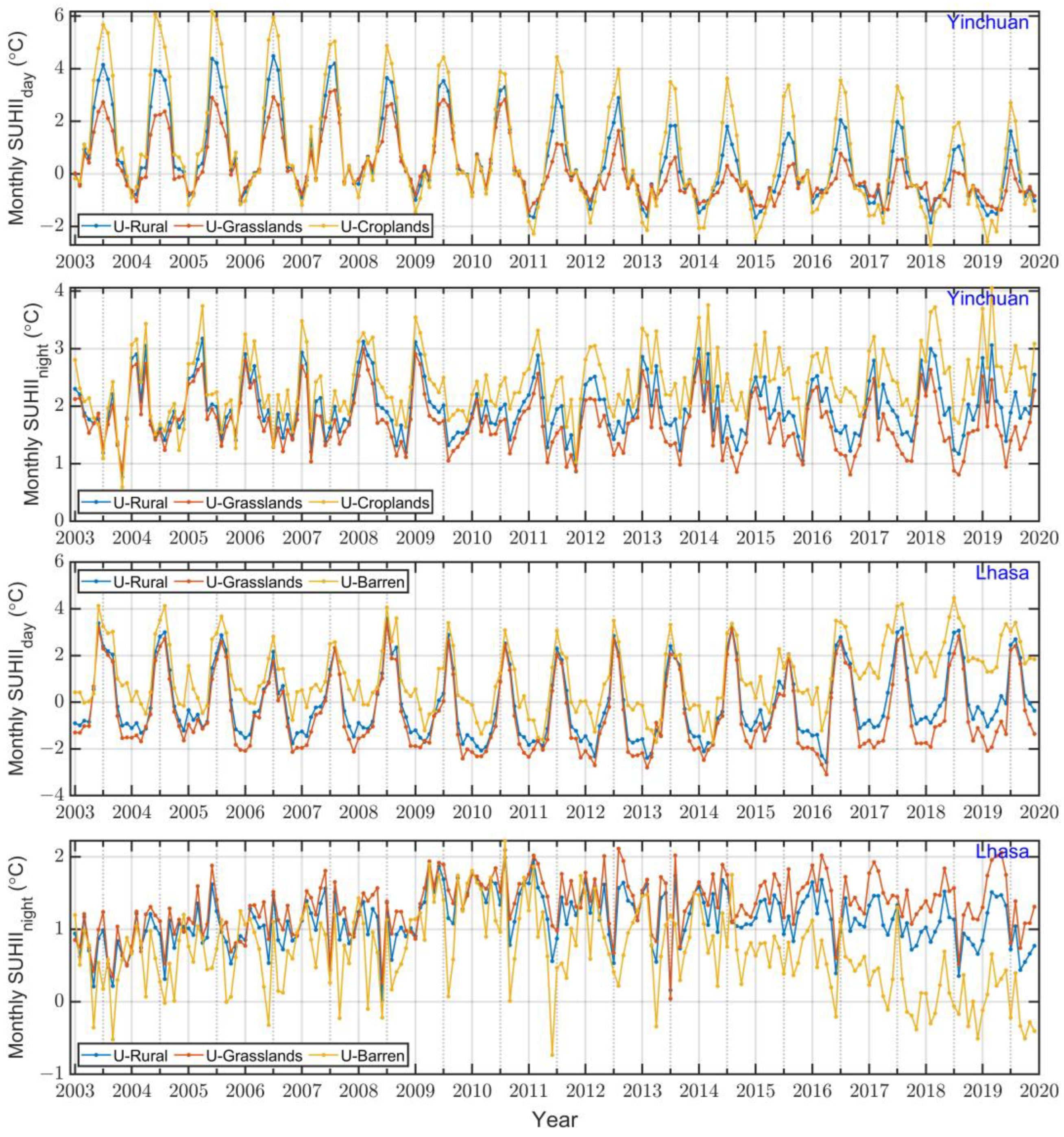
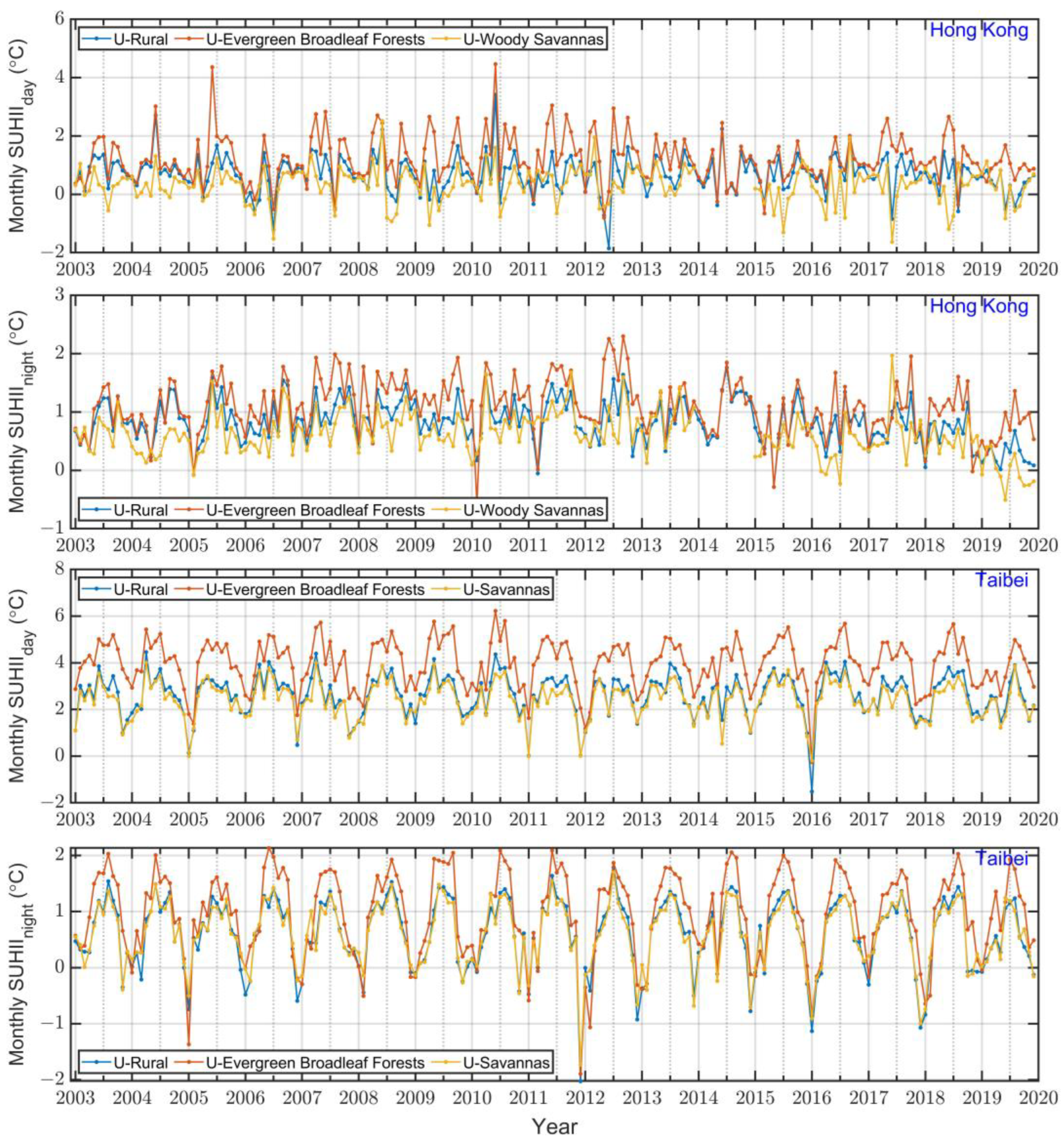
3.2.1. Comparison of Monthly SUHIIs

Pearson’s correlation coefficient was utilized to assess the correlation between daytime and nighttime SUHII and SUHII1 and SUHII2. Scatter plots of SUHII and SUHII1/SUHII2 are presented in Figure 4 and Figure 5 for daytime and nighttime, respectively. During the daytime, the correlation coefficients of SUHII and SUHII1/SUHII2 in most UAs are above 0.9, except for Xining in the northwest region and Hong Kong in the southeast region. At nighttime, the correlation coefficients of SUHII and SUHII1/SUHII2 in each city are all above 0.9, except for SUHII2 calculated by cropland in Lhasa, and SUHII1 and SUHII2 calculated by evergreen broadleaf forests and savannas, respectively, in Hong Kong. Overall, the difference between SUHII and SUHII1/SUHII2 in 34 major UAs in China is negligible, except for UAs with mixed rural land cover types.
During the daytime, the LST is primarily influenced by vegetation activities. In the northwest region, where grassland and cropland dominate rural areas, the SUHII1 compared to SUHII2, was more similar to SUHII (Figure 4). However, in UAs like Yinchuan, SUHII2 is underestimated in low-value regions and overestimated in high-value regions compared to SUHII, possibly due to seasonal variations in vegetation activity. As the high and low-value regions correspond to different growth seasons of vegetation, the rural LST is lower in the season of vigorous vegetation activity, which resulted in a greater SUHII2, and vice versa. Similarly, in Lhasa, which is located at a high altitude, the surrounding farming and pastoral areas are dominated by grassland and barren, where the proportion of grassland has increased in recent years [38]. Under normal circumstances, the LST of barren land is higher than that of urban surface and green space [21], while the LST of bare rock may be lower in Lhasa, which is located on the Tibetan Plateau, due to factors such as topography and altitude [39]; thus, the daytime SUHII2 is overestimated compared to SUHII. In the Northeast region, the rural landcover types are all dominated by cropland, and there is little difference between SUHII1 and SUHII during the day. In Hong Kong and Taipei, the difference in vegetation activity led to an overestimation of daytime SUHII1 quantified by evergreen broadleaf forests, while daytime SUHII2 calculated with savanna was underestimated, compared to SUHIIs, respectively.
At nighttime, the influence of vegetation weakened, and factors like precipitation and surface roughness affected the surface sensible heat flux and surface heat storage that regulated the LST. It can be seen from Figure 5 that the difference between SUHII1 (estimated by grassland) and SUHII in Lhasa was not that obvious, while the SUHII2 by barren land is underestimated. The rough terrain of the bare rock surface in mountainous areas is more conducive to energy storage; thus, the lower nighttime LST leads to the lower SUHII2. Ningxia is located in the arid area of Northwest China, where the roughness of grassland is greater with higher aerodynamic resistance. Therefore, the LST of grassland at night is higher than that of cropland, which leads to overestimated SUHII2 [39,40]. In the Northeast region, the difference between nighttime SUHII1 and SUHII is not evident. In the southeast region, the difference between SUHII1 and SUHII2 at nighttime in Hong Kong and Taipei is lower compared with that at daytime, which is mainly due to the weakening of vegetation activities at night, and the reduced impact of evapotranspiration on rural LST. In Shanghai, the nighttime SUHII2 quantified by cropland is overestimated. Compared with savannas, it may be due to the higher roughness of the cropland and the larger aerodynamic impedance, which reduces the sensible heat flux; thus, the LST of the cropland at night is higher and leads to relatively lower SUHII.

3.2.2. Comparison of Long-Term Variation in Monthly SUHIIs

From 2003 to 2019, the monthly average daytime and nighttime SUHII of each city was calculated separately, and UAs with two components of principal rural land use types were picked out for comparison. The long-term variation for different quantifications of daytime and nighttime monthly SUHII is shown in Figure 6, Figure 7, Figure 8 and Figure 9. Among them, the blue curve is the SUHII quantified by the whole rural LST, and the orange-red and yellow curves are the SUHII1 and SUHII2, respectively.
In the Northwest region (Figure 6), the SUHII1 is underestimated and SUHII2 is overestimated compared to SUHII, both at daytime and nighttime in Yinchuan. In contrast, the SUHII1 is underestimated and SUHII2 is overestimated at daytime for Lhasa, and the opposite occurs at night.
In the Southeast region (Figure 7), the daytime SUHII1 calculated with the savanna and SUHII shows little difference, while the daytime SUHII2 calculated with the cropland is underestimated for Nanjing, Nanchang and Shanghai in summer. As shown in Figure 8, the nighttime SUHII1 is not underestimated in Nanjing and Shanghai, while nighttime SUHII2 is overestimated in Nanjing, Shanghai and Chongqing.
In the Southeast region (Figure 9), Hong Kong and Taipei, with evergreen broadleaf forests as the principal rural background and savanna as the secondary rural background, exhibit an obvious overestimation of daytime SUHII1, while there is an underestimation of daytime SUHII2 that is more pronounced in summer. At nighttime, the SUHII1 and SUHII2 are slightly different from SUHII in Hong Kong, while the SUHII1 in Taipei is overestimated.
In addition, in the northwest, southeast, and northeast regions, the difference between SUHII1 and SUHII2 is slight in some cities with grassland, savanna, and cropland as the single rural land use type, which is not investigated in detail here.

3.3. Spatiotemporal Patterns of Regional SUHII in China

3.3.1. Day–Night Cycle

To explore the day–night cycle of SUHII in China’s sub-regions, the SUHIIs obtained by Terra and Aqua at four times of the day were averaged for 34 UAs from 2003 to 2019. Figure 10 illustrates the day–night cycle of annual, summer, and winter-averaged SUHII. Generally, the day–night cycles derived from SUHII and SUHII1 were consistent for each region at a certain temporal scale.
In summer, the day–night variations of SUHII in the Northeast, Southeast regions, and the whole country are similar, peaking at 13:30 and reaching a minimum at nighttime (01:30 or 22:30). Conversely, the day–night variation in SUHII in the Northwest region is opposite, typically reaching its lowest value at 10:30 and gradually increasing at nighttime. At the same time, the magnitude is lower than in other regions. Since the UAs in the Northwest region are located in the arid zone, the pattern of day –night variation aligns with that in the global arid zone [20].
In winter, the day–night variation pattern of SUHII in the Southeast region mirrors that of summer, with peaks at 13:30 and a minimum at night (01:30 or 22:30). However, the absolute value of SUHII is lower in winter. Correspondingly, the Northwest region exhibits a similar pattern to summer, with the lowest values in the morning and increasing values at night. However, daytime SUHII in the Northwest region is generally lower than in summer, occasionally showing negative values indicative of cold islands. In the Northeast region, the day–night cycles of SUHII are similar to those of the whole country but opposite to the variations in summer. Here, SUHII reaches a minimum at noon (10:30 or 13:30) and gradually increases at night (01:30 or 22:30). This anomaly is attributed to stronger urban long-wave radiation at night due to severe pollution in winter, resulting in higher nighttime SUHII compared to daytime [13].

3.3.2. Monthly Variation

Figure 11 shows the variation in monthly average SUHII in China. Similar to the results in the diurnal cycle, the seasonal variations derived from monthly SUHII and SUHII1 were also consistent for each region at a certain temporal scale. The seasonal variation in daytime SUHII is more pronounced than that at night. During the daytime, SUHII reaches its highest value in July (or August) and drops to its lowest value in December (or January) for the whole country.
At nighttime, the monthly variations of SUHII are less obvious in each area. In autumn and winter, the nighttime SUHII in the Northeast and Northwest regions is higher than during the daytime, reaching its lowest value of the year in July and September. Conversely, nighttime SUHII in the Southeast region is lower than during the daytime throughout the year.
Comparing the upper and lower rows of Figure 11, it is apparent that the pattern of monthly variations by SUHII1 and SUHII are similar. This indicates that in regional-scale spatiotemporal analysis, the regional average SUHII quantified by the original “urban-rural temperature difference method” with entire rural reference is not affected by the diversification of rural landcover types and can accurately reveal the spatiotemporal patterns of regional SUHII.

3.3.3. Interannual Trend

From the foregoing analysis, the SUHII was hardly affected by the diversity of rural land use when reflecting its regional spatiotemporal pattern. On the annual average, summer, and winter average scales, respectively, the SUHII of 34 major UAs in China were averaged to obtain the inter-annual variation in SUHII across the country and for each geographic region, as shown in Figure 12, Figure 13 and Figure 14. The Mann–Kendal (MK) test was used to determine whether there is a significant interannual trend [41], and then the Sen’s slope (p < 0.05) was calculated [42].
As shown in Figure 12, on a national scale, the annual daytime SUHII presents no significant trend, while the annual nighttime SUHII shows a significant increasing trend (0.07 °C/decade). In the Northeast and Northwest regions, the nighttime SUHII increased significantly with slopes of 0.14 °C/decade and 0.10 °C/decade, respectively, while the daytime SUHII decreased significantly during the day (−0.31 °C/decade) in the Northwest region and increased significantly (0.24 °C/decade) in the Southeast region.
It can be seen from Figure 13 that on the summer scale, there is a significant increasing trend in daytime and nighttime SUHIIs with slopes of 0.11 °C/decade and 0.10 °C/decade, respectively, on a national scale. Concerning the inter-annual trends of daytime SUHI in each region, it decreased significantly in the Northwest region (−0.32 °C/decade) and increased significantly in the Southeast region (0.29 °C/decade). For nighttime SUHII, it increased significantly for the Northeast and Southeast regions with slopes of 0.14 °C/decade and 0.09 °C/decade, respectively.
It can be seen from Figure 14 that for the winter scale, there is no obvious change in the daytime, while the nighttime SUHII increases significantly (0.08 °C/decade) on the national scale. In the Northeast and Northwest regions, the daytime SUHII decreases significantly with slopes of −0.28 °C/decade and −0.34 °C/decade, respectively, while it increases significantly in the Southeast region (0.15 °C/decade). For nighttime SUHII, it increases significantly for the Northeast and Northwest regions with slopes of 0.25 °C/decade and 0.17 °C/decade, respectively. There was no obvious trend for nighttime SUHII in the Southeast region.

4. Discussion

The quantification of SUHII relies on distinguishing between rural and urban land surface temperatures (LST), which are influenced by land use and land cover (LULC) information. Given the typically minor variations in LST within urban clusters, accurately defining “rural” regions is crucial for SUHII quantification [23]. When rural regions exhibit a mix of LULC types, they may yield varying SUHII values for a single city, depending on the specific land cover types selected for reference [30]. However, it remains unclear how the SUHII values obtained using the entire rural area compare to those obtained using specific land cover categories. This issue, along with the feasibility of quantifying regional SUHII patterns using all rural LULC types and the potential impact of heterogeneous rural LST, has received limited attention in large-scale studies. In this study, we aimed to verify the reliability and feasibility of urban–rural difference methods in regional SUHI analysis. Understanding the effect of multiple rural land types on SUHII quantification under different rural backgrounds is crucial for clarifying these uncertainties.
Our results revealed that, in most UAs in China, the SUHII quantified using the entire rural area differed only slightly from SUHII1 and SUHII2, except in certain UAs with mixed rural land covers. Additionally, while there was a slight disparity in the monthly magnitude between SUHII and SUHII1 and SUHII2, the long-term patterns revealed by SUHII were not significantly affected by the diversity of rural landcover types. Moreover, according to the day–night cycle and seasonal variations integrated from the regional averages, the similar result of SUHII and SUHII1 further confirmed that the urban–rural method involving the whole rural region as a reference was feasible in the regional analysis of SUHI. The strong correlation between SUHII, SUHII1, and SUHII2 from single-city and regional scales, together with the analogous pattern of diurnal and seasonal SUHII and SUHII1, comprehensively verified the feasibility of the urban-rural LST difference method for large-scale regional SUHI analysis. The findings validate and supplement the previous uncertainties in the sensitivity of SUHI quantification under non-uniform rural background surfaces [21,23].
Given the feasibility of the urban–rural LST difference method in depicting regional SUHII patterns, our study identified significant spatial and temporal variations in SUHII across the Northeast, Northwest, and Southeast regions in China. Although consistency was found between the regional patterns of SUHII and SUHII1, this result is preliminary and limited to certain UAs in China. To extend the comparison of multiple SUHII indices to a global scale, future studies should consider quantifying SUHI under rural regions with more diverse land cover types and varied climate backgrounds to facilitate its applicability. Additionally, it is important to note that our SUHII measurements were based solely on clear-sky observations, which may lead to an overestimation of regional averaged results [43]. Therefore, the improved high-resolution LST was recommended in future SUHII studies at a regional scale.

5. Conclusions

The study comprehensively analyzed urban form expansion from 2003 to 2019 for 34 major UAs in China. Different quantifications of SUHII (SUHII1 and SUHII2) were then constructed by differentiating principal and secondary rural land cover types. These new quantification methods were compared with the original SUHII, based on the entire rural background, in terms of monthly average values and interannual variation. Finally, SUHII and SUHII1 were further compared in terms of the day–night cycle, monthly variation, and inter-annual trends across the country and in various geographic regions. These analyses of SUHIIs from multiple spatial and temporal aspects affirmed the reliability of the traditional urban-rural LST difference method in exploring regional SUHII patterns. Moreover, the study investigated the spatiotemporal dynamics of SUHII in China.
The main conclusions are as follows:
(1)
Among the 34 UAs in China, 32 UAs other than Lanzhou and Lhasa experienced significant urban expansion accompanied by changes in surrounding rural land use types during 2003–2019, underscoring the significance of defining the dynamic urban–rural extent in SUHII quantification.
(2)
Considering different SUHII quantifications at each UA, the long-term variation in monthly SUHII and SUHII1/SUHII2 showed identical trends with strong correlation coefficients of over 0.9 in most (32) UAs but with varying magnitudes in certain arid UAs.
(3)
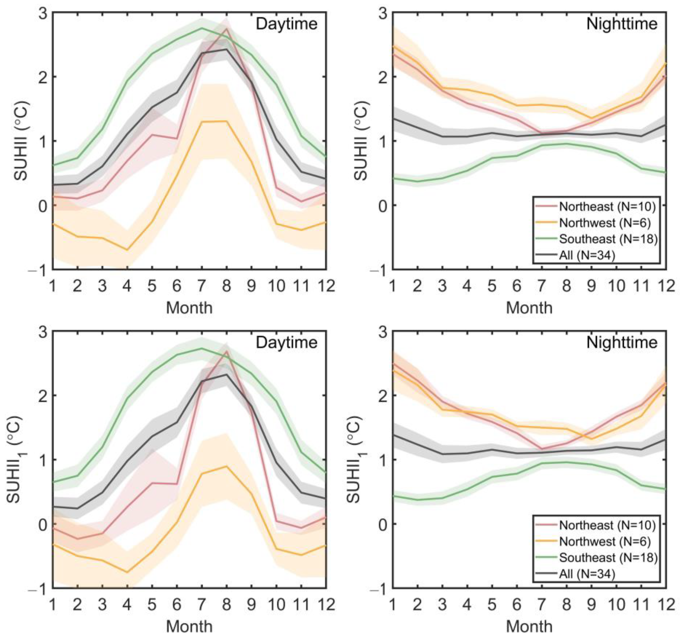
The regional patterns of diurnal and monthly SUHIIs revealed by considering the entire rural area, in Northeast, Northwest, and Southeast China, respectively, are not influenced by the diversity of rural land covers.
(4)
Seasonal SUHII exhibits disparities in day–night variation and regional contrast in China. In summer, SUHII peaks at noon and decreases at night, exhibiting the opposite pattern in the northwest region. Conversely, in winter, SUHII is lowest at noon and rises at night for most regions, with the southeast region displaying the opposite trend.
(5)
The monthly variation in daytime SUHII is more pronounced than that at night. Nationally, daytime SUHII peaks in July (or August) and reaches its lowest point in December (or January), with nighttime values remaining relatively stable across geographical regions.
(6)
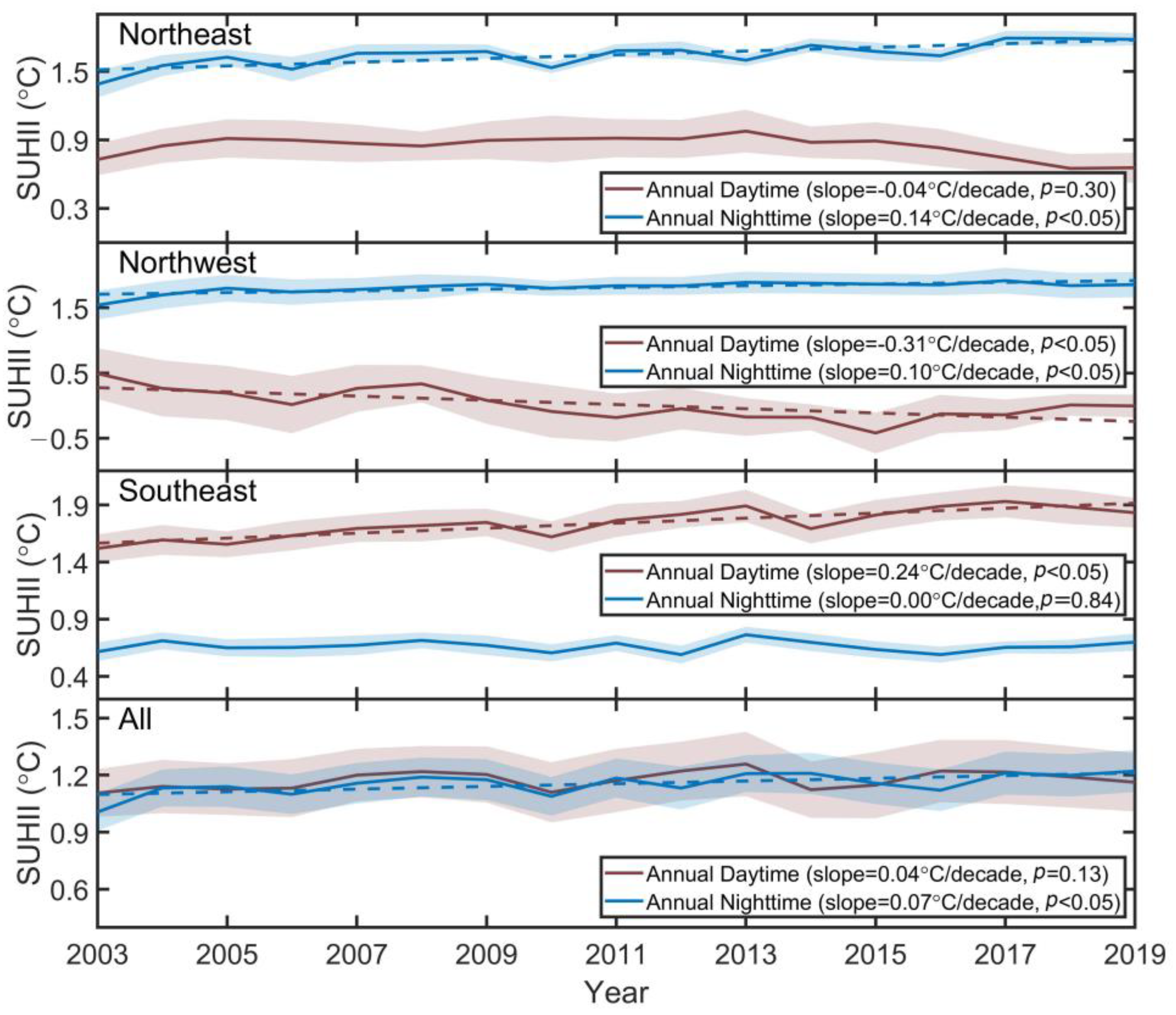
Interannual trends of SUHII vary across different regions. On a national scale, there is no significant trend in annual daytime SUHII from 2003 to 2019, while nighttime SUHII shows a steady increase at a rate of 0.07 °C/decade. Both summer daytime and nighttime SUHII exhibit significant increasing trends, with rates of 0.11 °C/decade and 0.10 °C/decade, respectively. Notably, there is a significant increasing trend (0.08 °C/decade) for winter nighttime SUHII.

Author Contributions

Conceptualization, M.S. and Z.-L.L.; methodology, M.S.; validation, M.S., N.Y. and X.L.; writing—original draft preparation, M.S.; writing—review and editing, M.S. and N.Y.; supervision, B.-H.T. and F.N. All authors have read and agreed to the published version of the manuscript.

Funding

This research was funded by the National Natural Science Foundation of China, grant number 42201404 and 41921001, and the China Postdoctoral Science Foundation, grant number 2022M723439.

Data Availability Statement

The MODIS LST and landcover type datasets and the elevation data from GTOPO30 are freely available from the Google Earth Engine platform.

Acknowledgments

We would like to acknowledge the Google Earth Engine platform for providing MODIS and topographic data free of charge.

Conflicts of Interest

The authors declare no conflicts of interest.

References

  1. Clinton, N.; Gong, P. MODIS detected surface urban heat islands and sinks: Global locations and controls. Remote Sens. Environ. 2013, 134, 294–304. [Google Scholar] [CrossRef]
  2. Peng, S.; Piao, S.; Ciais, P.; Friedlingstein, P.; Ottle, C.; Bréon, F.-M.; Nan, H.; Zhou, L.; Myneni, R.B. Surface Urban Heat Island Across 419 Global Big Cities. Environ. Sci. Technol. 2012, 46, 696–703. [Google Scholar] [CrossRef] [PubMed]
  3. Oke, T.R. The energetic basis of the urban heat island. Q. J. R. Meteorol. Soc. 1982, 108, 1–24. [Google Scholar] [CrossRef]
  4. Zhao, S.; Liu, S.; Zhou, D. Prevalent vegetation growth enhancement in urban environment. Proc. Natl. Acad. Sci. USA 2016, 113, 6313. [Google Scholar] [CrossRef]
  5. Grimm, N.B.; Faeth, S.H.; Golubiewski, N.E.; Redman, C.L.; Wu, J.; Bai, X.; Briggs, J.M. Global change and the ecology of cities. Science 2008, 319, 756–760. [Google Scholar] [CrossRef] [PubMed]
  6. Bai, X.; Dawson, R.J.; Ürge-Vorsatz, D.; Delgado, G.C.; Salisu Barau, A.; Dhakal, S.; Dodman, D.; Leonardsen, L.; Masson-Delmotte, V.; Roberts, D.C.; et al. Six research priorities for cities and climate change. Nature 2018, 555, 23–25. [Google Scholar] [CrossRef]
  7. Patz, J.A.; Campbell-Lendrum, D.; Holloway, T.; Foley, J.A. Impact of regional climate change on human health. Nature 2005, 438, 310–317. [Google Scholar] [CrossRef]
  8. O’Loughlin, J.; Witmer, F.D.W.; Linke, A.M.; Laing, A.; Gettelman, A.; Dudhia, J. Climate variability and conflict risk in East Africa, 1990–2009. Proc. Natl. Acad. Sci. USA 2012, 109, 18344. [Google Scholar] [CrossRef] [PubMed]
  9. Kalnay, E.; Cai, M. Impact of urbanization and land-use. Nature 2003, 425, 102. [Google Scholar] [CrossRef]
  10. Zhou, D.; Xiao, J.; Bonafoni, S.; Berger, C.; Deilami, K.; Zhou, Y.; Frolking, S.; Yao, R.; Qiao, Z.; Sobrino, J.A. Satellite remote sensing of surface urban heat islands: Progress, challenges, and perspectives. Remote Sens. 2019, 11, 48. [Google Scholar] [CrossRef]
  11. Du, Y.; Xie, Z.Q.; Zhang, L.L.; Wang, N.; Wang, M.; Hu, J.W. Machine-Learning-Assisted Characterization of Regional Heat Islands with a Spatial Extent Larger than the Urban Size. Remote Sens. 2024, 16, 20. [Google Scholar] [CrossRef]
  12. Li, Z.-L.; Si, M.; Leng, P. A review of remotely sensed surface urban heat islands from the fresh perspective of comparisons among different regions (Invited Review). Prog. Electromagn. Res. C 2020, 102, 31–46. [Google Scholar] [CrossRef]
  13. Zhou, D.; Zhao, S.; Liu, S.; Zhang, L.; Zhu, C. Surface urban heat island in China’s 32 major cities: Spatial patterns and drivers. Remote Sens. Environ. 2014, 152, 51–61. [Google Scholar] [CrossRef]
  14. Peng, J.; Jia, J.; Liu, Y.; Li, H.; Wu, J. Seasonal contrast of the dominant factors for spatial distribution of land surface temperature in urban areas. Remote Sens. Environ. 2018, 215, 255–267. [Google Scholar] [CrossRef]
  15. Zhang, P.; Imhoff, M.L.; Wolfe, R.E.; Bounoua, L. Characterizing urban heat islands of global settlements using MODIS and nighttime lights products. Can. J. Remote Sens. 2010, 36, 185–196. [Google Scholar] [CrossRef]
  16. Yu, Z.; Yao, Y.; Yang, G.; Wang, X.; Vejre, H. Spatiotemporal patterns and characteristics of remotely sensed region heat islands during the rapid urbanization (1995–2015) of Southern China. Sci. Total Environ. 2019, 674, 242–254. [Google Scholar] [CrossRef] [PubMed]
  17. Deilami, K.; Kamruzzaman, M.; Liu, Y. Urban heat island effect: A systematic review of spatio-temporal factors, data, methods, and mitigation measures. Int. J. Appl. Earth Obs. Geoinf. 2018, 67, 30–42. [Google Scholar] [CrossRef]
  18. Zhou, D.; Zhao, S.; Zhang, L.; Sun, G.; Liu, Y. The footprint of urban heat island effect in China. Sci. Rep. 2015, 5, 2–12. [Google Scholar] [CrossRef]
  19. Chakraborty, T.; Lee, X. A simplified urban-extent algorithm to characterize surface urban heat islands on a global scale and examine vegetation control on their spatiotemporal variability. Int. J. Appl. Earth Obs. Geoinf. 2019, 74, 269–280. [Google Scholar] [CrossRef]
  20. Si, M.; Li, Z.-L.; Nerry, F.; Tang, B.-H.; Leng, P.; Wu, H.; Zhang, X.; Shang, G. Spatiotemporal pattern and long-term trend of global surface urban heat islands characterized by dynamic urban-extent method and MODIS data. ISPRS J. Photogramm. 2022, 183, 321–335. [Google Scholar] [CrossRef]
  21. Haashemi, S.; Weng, Q.; Darvishi, A.; Alavipanah, S.K. Seasonal variations of the surface urban heat Island in a semi-arid city. Remote Sens. 2016, 8, 352. [Google Scholar] [CrossRef]
  22. Patel, S.; Indraganti, M.; Jawarneh, R.N. A comprehensive systematic review: Impact of Land Use/ Land Cover (LULC) on Land Surface Temperatures (LST) and outdoor thermal comfort. Build. Environ. 2024, 249, 13. [Google Scholar] [CrossRef]
  23. Martin-Vide, J.; Sarricolea, P.; Moreno-García, M.C. On the definition of urban heat island intensity: The “rural” reference. Front. Earth Sci. 2015, 3, 24. [Google Scholar] [CrossRef]
  24. Zhao, S.; Zhou, D.; Liu, S. Data concurrency is required for estimating urban heat island intensity. Environ. Pollut. 2016, 208, 118–124. [Google Scholar] [CrossRef] [PubMed]
  25. Song, W.; Deng, X.Z. Land-use/land-cover change and ecosystem service provision in China. Sci. Total Environ. 2017, 576, 705–719. [Google Scholar] [CrossRef] [PubMed]
  26. Liu, Y.S. Introduction to land use and rural sustainability in China. Land Use Policy 2018, 74, 1–4. [Google Scholar] [CrossRef]
  27. Yao, R.; Wang, L.; Huang, X.; Liu, Y.; Niu, Z.; Wang, S.; Wang, L. Long-term trends of surface and canopy layer urban heat island intensity in 272 cities in the mainland of China. Sci. Total Environ. 2021, 772, 145607. [Google Scholar] [CrossRef] [PubMed]
  28. Si, M.; Li, Z.-L.; Tang, B.-H.; Liu, X.; Nerry, F. Spatial heterogeneity of driving factors-induced impacts for global long-term surface urban heat island. Int. J. Remote Sens. 2023, 1–21. [Google Scholar] [CrossRef]
  29. Zhou, D.; Xiao, J.; Frolking, S.; Zhang, L.; Zhou, G. Urbanization Contributes Little to Global Warming but Substantially Intensifies Local and Regional Land Surface Warming. Earth’s Future 2022, 10, e2021EF002401. [Google Scholar] [CrossRef]
  30. Zhou, D.; Zhang, L.; Li, D.; Huang, D.; Zhu, C. Climate-vegetation control on the diurnal and seasonal variations of surface urban heat islands in China. Environ. Res. Lett. 2016, 11, 074009. [Google Scholar] [CrossRef]
  31. Li, X.C.; Liu, S.R.; Ma, Q.W.; Cao, W.T.; Zhang, H.G.; Wang, Z.H. Impacts of spatial explanatory variables on surface urban heat island intensity between urban and suburban regions in China. Int. J. Digit. Earth 2024, 17, 17. [Google Scholar] [CrossRef]
  32. Fang, J.; Chen, A.; Peng, C.; Zhao, S.; Ci, L. Changes in Forest Biomass Carbon Storage in China between 1949 and 1998. Science 2001, 292, 2320–2322. [Google Scholar] [CrossRef] [PubMed]
  33. Wu, X.; Wang, G.; Yao, R.; Wang, L.; Yu, D.; Gui, X. Investigating Surface Urban Heat Islands in South America Based on MODIS Data from 2003–2016. Remote Sens. 2019, 11, 1212. [Google Scholar] [CrossRef]
  34. Simwanda, M.; Ranagalage, M.; Estoque, R.C.; Murayama, Y. Spatial Analysis of Surface Urban Heat Islands in Four Rapidly Growing African Cities. Remote Sens. 2019, 11, 1645. [Google Scholar] [CrossRef]
  35. Mansourmoghaddam, M.; Rousta, I.; Malamiri, H.G.; Sadeghnejad, M.; Krzyszczak, J.; Ferreira, C.S.S. Modeling and Estimating the Land Surface Temperature (LST) Using Remote Sensing and Machine Learning (Case Study: Yazd, Iran). Remote Sens. 2024, 16, 24. [Google Scholar] [CrossRef]
  36. Sulla-Menashe, D.; Friedl, M.A. User Guide to Collection 6 MODIS Land Cover (MCD12Q1 and MCD12C1) Product; USGS: Reston, VA, USA, 2018; pp. 1–18. [Google Scholar]
  37. Rozenfeld, H.D.; Rybski, D.; Andrade, J.S.; Batty, M.; Stanley, H.E.; Makse, H.A. Laws of population growth. Proc. Natl. Acad. Sci. USA 2008, 105, 18702–18707. [Google Scholar] [CrossRef] [PubMed]
  38. Gao, J.; Huang, X.; Ni, M. Spatio-temporal distribution of heat island effect in Lhasa and its response to land-use/cover in 2012-2016. Meteorological 2018, 44, 936–943. [Google Scholar]
  39. Wen, L.; Peng, W.; Yang, H.; Wang, H.; Dong, L.; Shang, X. An analysis of land surface temperature (LST) and its influencing factors in summer in western Sichuan Plateau: A case study of Xichang City. Remote Sens. Land Resour. 2017, 29, 207–214. [Google Scholar]
  40. Xie, M.; Wang, Y.; Fu, M. An Overview and Perspective about Causative Factors of Surface Urban Heat Island Effects. Progress Geogr. 2011, 30, 35–41. [Google Scholar]
  41. Fernandes, R.; Leblanc, S.G. Parametric (modified least squares) and non-parametric (Theil–Sen) linear regressions for predicting biophysical parameters in the presence of measurement errors. Remote Sens. Environ. 2005, 95, 303–316. [Google Scholar] [CrossRef]
  42. Mondal, A.; Khare, D.; Kundu, S. Spatial and temporal analysis of rainfall and temperature trend of India. Theor. Appl. Climatol. 2015, 122, 143–158. [Google Scholar] [CrossRef]
  43. Yang, Q.Q.; Xu, Y.; Wen, D.W.; Hu, T.; Chakraborty, T.; Liu, Y.; Yao, R.; Chen, S.R.; Xiao, C.J.; Yang, J. Satellite Clear-Sky Observations Overestimate Surface Urban Heat Islands in Humid Cities. Geophys. Res. Lett. 2024, 51, 10. [Google Scholar] [CrossRef]
Figure 1. The spatial distribution of 34 Chinese urban agglomerations, indicating their principal (numbers in red color) and/or secondary (numbers in blue color) rural land types. The labels in each city center are their abbreviation name as defined in the main text.
Remotesensing 16 01232 g001
Figure 2. Spatial variations of urban morphology of 34 Chinese urban agglomerations during 2003 and 2019. The boundaries were delineated with a city clustering algorithm based on LULC data (details in Section 2.3).
Remotesensing 16 01232 g002
Figure 3. Urban area and expanding rates for 34 Chinese urban agglomerations during 2003 and 2019. The changing rate was calculated by the Sen’s Slope at 95% significance intervals. The abbreviations of urban names in X axis corresponds to the definition in Section 2.1.
Remotesensing 16 01232 g003
Figure 4. Comparison of monthly daytime SUHIIs (Y-axis) quantified by primary (SUHI1) and secondary (SUHI2) rural components, with traditional SUHII by whole rural region (X-axis). The U-x points in orange and blue colors represent the values of SUHI1 and SUHI2, respectively.
Remotesensing 16 01232 g004
Figure 5. Comparison of monthly daytime SUHIIs (Y-axis) quantified by primary (SUHI1) and secondary (SUHI2) rural components, with traditional SUHII by whole rural region (X-axis). The U-x points in orange and blue colors represent the values of SUHI1 and SUHI2, respectively.
Remotesensing 16 01232 g005
Figure 6. Long-term trend of monthly daytime and nighttime SUHIIs during 2003 and 2019 in several of Northwest China’s urban agglomerations (mainly grasslands, croplands and barren in rural).
Remotesensing 16 01232 g006
Figure 7. Long-term trend of monthly daytime SUHIIs between 2003 and 2019 in several of Southeast China’s urban agglomerations (mainly croplands and savannas in rural).
Remotesensing 16 01232 g007
Figure 8. Long-term trend of monthly nighttime SUHIIs between 2003 and 2019 in several of Southeast China’s urban agglomerations (mainly croplands and savannas in rural).
Remotesensing 16 01232 g008
Figure 9. Long-term trend of monthly daytime and nighttime SUHIIs between 2003 and 2019 in several of Southeast China’s urban agglomerations (mainly evergreen broadleaf forests and savannas in rural).
Remotesensing 16 01232 g009
Figure 10. Day–night cycles of annual, summer and winter-averaged SUHII and SUHII1 in China’s sub-regions. The solid lines denote the mean values, and the error bars represent its standard errors.
Remotesensing 16 01232 g010
Figure 11. Variations of daytime and nighttime monthly SUHII (SUHII and SUHII1) in China’s sub-regions. The mean value is denoted in solid lines, and its standard errors are in shaded patches.
Remotesensing 16 01232 g011
Figure 12. Inter-annual variations of annual daytime and nighttime SUHII for China’s sub-regions over the period 2003–2019. The solid line depicts the mean value of each year, and its standard errors are in the shaded patch. The Sen’s slope is calculated at a 95% significant interval. The variations with significant linear trends are delineated with dashed lines in all sub-figures.
Remotesensing 16 01232 g012
Figure 13. Inter-annual variations of summer daytime and nighttime SUHII for China’s sub-regions over the period 2003–2019. The solid line depicts the mean value of each year, and its standard errors are in the shaded patch. The Sen’s slope is calculated at a 95% significant interval. The variations with significant trends are delineated with a dashed line. The variations with significant linear trends are delineated with dashed lines in all sub-figures.
Remotesensing 16 01232 g013
Figure 14. Inter-annual variations of winter daytime and nighttime SUHII for China’s sub-regions over the period 2003–2019. The solid line depicts the mean value of each year, and its standard errors are in the shaded patch. The Sen’s slope is calculated at a 95% significant interval. The variations with significant trends are delineated in the dashed line. The variations with significant linear trends are delineated with dashed lines in all sub-figures.
Remotesensing 16 01232 g014
Table 1. IGBP legend and classification for MCD12Q1.
ValueNameDescription
1Evergreen Needleleaf ForestsDominated by evergreen conifer trees (canopy > 2 m). Tree cover > 60%.
2Evergreen Broadleaf ForestsDominated by evergreen broadleaf and palmate trees (canopy > 2 m). Tree cover > 60%.
3Deciduous Needleleaf ForestsDominated by deciduous needleleaf (larch) trees (canopy > 2 m). Tree cover > 60%.
4Deciduous Broadleaf ForestsDominated by deciduous broadleaf trees (canopy > 2 m). Tree cover > 60%.
5Mixed ForestsDominated by neither deciduous nor evergreen (40–60% of each) tree type (canopy > 2 m). Tree cover > 60%.
6Closed ShrublandsDominated by neither deciduous nor evergreen (40–60% of each) tree type (canopy > 2 m). Tree cover > 60%.
7Open ShrublandsDominated by woody perennials (1–2 m height) 10–60% cover.
8Woody SavannasTree cover 30–60% (canopy > 2 m).
9SavannasTree cover 10–30% (canopy > 2 m).
10GrasslandsDominated by herbaceous annuals (<2 m).
11Permanent WetlandsPermanently inundated lands with 30–60% water cover and >10% vegetated cover.
12CroplandsAt least 60% of the area is cultivated cropland.
13Urban and Built-up LandsAt least 30% impervious surface area, including building materials, asphalt, and vehicles.
14Cropland/Natural Vegetation MosaicsMosaics of small-scale cultivation 40–60% with natural tree, shrub, or herbaceous vegetation.
15Permanent Snow and IceAt least 60% of the area is covered by snow and ice for at least 10 months of the year.
16BarrenAt least 60% of the area is non-vegetated barren (sand, rock, soil) areas with less than 10% vegetation.
17Water BodiesAt least 60% of the area is covered by permanent water bodies.
Disclaimer/Publisher’s Note: The statements, opinions and data contained in all publications are solely those of the individual author(s) and contributor(s) and not of MDPI and/or the editor(s). MDPI and/or the editor(s) disclaim responsibility for any injury to people or property resulting from any ideas, methods, instructions or products referred to in the content.

