Revealing Decadal Glacial Changes and Lake Evolution in the Cordillera Real, Bolivia: A Semi-Automated Landsat Imagery Analysis

Abstract

The impact of global climate change on glaciers has drawn significant attention; however, limited research has been conducted to comprehend the consequences of glacier melting on the associated formation and evolution of glacial lakes. This study presents a semi-automated methodology developed on the cloud platforms Google Earth Engine and Google Colab to effectively detect dynamic changes in the glaciers as well as glacial and non-glacial lakes of the Cordillera Real, Bolivia, using over 200 Landsat images from 1984 to 2021. We found that the study area experienced a rise in temperature and precipitation, resulting in a substantial decline in glacier coverage and a simultaneous increase in both the total number and total area of lakes. A strong correlation between glacier area and the extent of natural glacier-fed lakes highlights the significant downstream impact of glacier recession on water bodies. Over the study period, glaciers reduced their total area by 42%, with recent years showing a deceleration in glacier recession, aligning with the recent stabilization observed in the area of natural glacier-fed lakes. Despite these overall trends, many smaller lakes, especially non-glacier-fed ones, decreased in size, attributed to seasonal and inter-annual variations in lake inflow caused by climate variability. These findings suggest the potential decline of natural lakes amid ongoing climate changes, prompting alterations in natural landscapes and local water resources. The study reveals the response of glaciers and lakes to climate variations, including the contribution of human-constructed water reservoirs, providing valuable insights into crucial aspects of future water resources in the Cordillera Real.

1. Introduction

Glaciers serve as invaluable natural freshwater reservoirs for downstream regions worldwide, with glacial meltwater playing a significant role in various functions, including domestic use, agriculture, hydropower generation, and environmental health [1,2]. As global warming persists and precipitation patterns become more variable, the accelerated melting and retreat of glaciers, dramatically reshape the hydrological systems and ecological landscapes. This is of particular importance for tropical glaciers, especially in the tropical Andes where more than 99% of tropical glaciers are located [3], due to the vulnerability of glaciers to climate change and the significant cumulative specific mass reductions they have experienced since the 1960s [4,5], with even more pronounced retreat observed in small glaciers at lower elevations [6]. This further leads to the emergence of new lakes and wetlands, profoundly affecting water availability, ecosystems, and the susceptibility to disasters in the region. While numerous studies related to tropical glaciers primarily focus on the glacier dynamics, glacial runoff, and the risk of glacial lake outburst floods (GLOF) [6,7,8,9,10,11,12,13,14,15,16,17,18], there remains a substantial deficiency in the comprehensive understanding of lake evolution in this region [19]. Moreover, the analysis of spatiotemporal changes in the multitude of glacial lakes and their potential implications for water resources is notably lacking, although obtaining continuous lake dynamics records would help explore the relationship between key hydrological factors, including precipitation and supply of meltwater from glaciers, and lake evolution patterns [20]. This highlights the critical need for a precise and rapid method to effectively capture changes in glaciers and lakes and their interactions. Such an approach is essential to conduct comprehensive research aimed at understanding the dynamic nature of these water bodies and the intricate interplay of critical climate change factors impacting them.

Due to the difficulty in reaching high-altitude regions [17] and the low availability and high cost of field measurement, satellite images are more frequently used for the analysis of glaciers and glacial lakes and observing their long-term variations in the Andes [12]. The traditional methods for mapping glaciers and glacial lakes in mountainous regions involve using the band ratio method [21], Normalized Difference Snow Index (NDSI) [22], and Normalized Difference Water Index (NDWI) [23] images with manually selected thresholds. Lately, pixel-wised classification utilizing machine learning methods has relieved the burden of manual operation [24,25,26]. Yet, current methodologies in glacier mapping still encounter challenges, including incorrectly mapping seasonal snow and misclassifying cloud cover and shadows cast by the steep terrain as glaciers [27]. Similar defects exist in the mapping of glacial lakes, where these methods confront issues such as misclassifying shadows as lakes and being unable to capture spatial information such as pixel proximity and the geometric characteristics of classes, which is crucial for effective water classification. Hence, there is a strong demand for a robust methodology to conduct a comprehensive analysis of glaciers and glacial lakes using satellite imagery. Such a methodology should address potential accuracy limitations stemming from resolution constraints, mountain shadow influences, and the selection of detection methods, all of which impact the subsequent analysis and discussion concerning the formation and advancement of glacier lakes, their interaction with glaciers, and their relationship with climate variability.

With this background, this study primarily focuses on unveiling the spatiotemporal changes in glaciers and lakes, encompassing approximately four decades from 1984 to 2021 within the tropical Andes and specifically focusing on the Cordillera Real region of Bolivia. This is achieved by utilizing the cloud platforms Google Earth Engine (GEE) and Google Colab. The study involves developing a semi-automatic method for mapping glaciers and lakes, significantly reducing manual work while ensuring process efficiency and accuracy.

In addition to comprehending the dynamic nature and interconnectedness of glaciers and glacial lakes, our investigation aims to explore the influence of critical climate change factors, including temperature and precipitation, in conjunction with human activities, on the observed transformations in these water bodies. Through this comprehensive analysis, our goal is to bridge the gap in understanding the changes of lakes in the tropical Andes and elucidate the implications of these evolutions on the region’s water resources and environment for the future.

2. Materials and Methods

2.1. Study Region

The Cordillera Real is a glacierized mountain range located in Northwest Bolivia, South America, separating the cold arid Altiplano Plateau from the wet warm Amazon Basin. Consistent with the previous study [28], smaller glacierized areas to the further south, Mururata, and Illimani are included in this study, as shown in Figure 1.

The maximum glacier extent occurred in the second half of the 17th century, followed by nearly continuous retreat since the mid-18th century [29]. Global Land Ice Measurements From Space (GLIMS) [30] encompasses 289 records of glaciers which start to appear around 4500 m.a.s.l in the study region, with the data from 2000 collectively covering an area of around 275 km². As part of the outer tropics, ablation of the glaciers in the Cordillera Real occurs year-round while accumulation is confined to the wet season (from October to March) [31]. The equilibrium line altitude (ELA), where the rate of ice accumulation equals the rate of ice loss at this elevation, is measured at a benchmark glacier of the World Glacier Monitoring Service (WGMS), i.e., the Zongo glacier, and was 5144 ± 67 m.a.s.l. during 1991–2006 [32].

Under the influence of high solar radiation and low glacier albedo, meltwater discharge reaches its peak annual values in November–December [14]. The runoff from glacierized basins, flowing into large lakes like Lake Tuni and Lake Milluni, significantly contributes to the drinking water systems that cater to the needs of La Paz and El Alto, two major cities in Bolivia [10]. As lakes supplied by glacier meltwaters can have a certain distance from the glacier margins [33], this study considered the region above 4300 m.a.s.l. to encompass the major lakes in the study region, including Lake Tuni and Lake Milluni.

2.2. Data

Landsat 5 and Landsat 8 Collection 2 Tier 1 calibrated top-of-atmosphere (TOA) reflectance data from 1984 to 2021 were accessed from the GEE platform (https://developers.google.com/earth-engine/datasets/catalog/landsat, accessed on 1 June 2022). The cloud cover rate in the study region was determined using the quality assessment band in the Landsat images, calculated through the C Function of Mask (CFMask) algorithm [34]. To mitigate cloud interference, 51 images with a cloud cover rate of less than 15% (

Table A1. List of Landsat images with a cloud cover rate smaller than 15%.

Date of Image Acquisition	Image ID	Date of Image Acquisition	Image ID
1988/6/17	LT05_L1TP_001071_19880617_20200917_02_T1	2009/5/26	LT05_L1TP_001071_20090526_20200827_02_T1
1988/7/3	LT05_L1TP_001071_19880703_20200917_02_T1	2009/6/11	LT05_L1TP_001071_20090611_20200827_02_T1
1988/7/19	LT05_L1TP_001071_19880719_20200917_02_T1	2009/6/27	LT05_L1TP_001071_20090627_20200827_02_T1
1988/8/20	LT05_L1TP_001071_19880820_20200917_02_T1	2010/5/13	LT05_L1TP_001071_20100513_20200824_02_T1
1991/5/25	LT05_L1TP_001071_19910525_20230519_02_T1	2010/6/14	LT05_L1TP_001071_20100614_20200824_02_T1
1992/5/11	LT05_L1TP_001071_19920511_20200914_02_T1	2010/8/17	LT05_L1TP_001071_20100817_20200824_02_T1
1992/5/27	LT05_L1TP_001071_19920527_20200914_02_T1	2010/10/4	LT05_L1TP_001071_20101004_20200823_02_T1
1992/6/12	LT05_L1TP_001071_19920612_20200914_02_T1	2011/5/16	LT05_L1TP_001071_20110516_20200822_02_T1
1994/6/2	LT05_L1TP_001071_19940602_20200913_02_T1	2014/7/11	LC08_L1TP_001071_20140711_20200911_02_T1
1994/7/20	LT05_L1TP_001071_19940720_20200913_02_T1	2015/6/28	LC08_L1TP_001071_20150628_20200909_02_T1
1995/6/5	LT05_L1TP_001071_19950605_20200912_02_T1	2015/7/30	LC08_L1TP_001071_20150730_20200908_02_T1
1995/6/21	LT05_L1TP_001071_19950621_20200913_02_T1	2016/5/29	LC08_L1TP_001071_20160529_20200906_02_T1
1995/8/8	LT05_L1TP_001071_19950808_20200912_02_T1	2016/8/1	LC08_L1TP_001071_20160801_20200906_02_T1
1996/5/22	LT05_L1TP_001071_19960522_20200911_02_T1	2017/7/19	LC08_L1TP_001071_20170719_20200903_02_T1
1999/7/2	LT05_L1TP_001071_19990702_20200907_02_T1	2017/8/4	LC08_L1TP_001071_20170804_20200903_02_T1
2000/8/5	LT05_L1TP_001071_20000805_20200906_02_T1	2017/8/20	LC08_L1TP_001071_20170820_20200903_02_T1
2003/6/27	LT05_L1TP_001071_20030627_20200905_02_T1	2019/6/7	LC08_L1TP_001071_20190607_20200828_02_T1
2004/4/26	LT05_L1TP_001071_20040426_20200903_02_T1	2019/6/23	LC08_L1TP_001071_20190623_20200827_02_T1
2004/5/28	LT05_L1TP_001071_20040528_20200903_02_T1	2019/7/9	LC08_L1TP_001071_20190709_20200827_02_T1
2005/4/29	LT05_L1TP_001071_20050429_20200902_02_T1	2020/5/24	LC08_L1TP_001071_20200524_20200820_02_T1
2005/6/16	LT05_L1TP_001071_20050616_20200902_02_T1	2020/6/9	LC08_L1TP_001071_20200609_20200824_02_T1
2005/9/4	LT05_L1TP_001071_20050904_20200901_02_T1	2020/6/25	LC08_L1TP_001071_20200625_20200823_02_T1
2006/6/19	LT05_L1TP_001071_20060619_20200831_02_T1	2020/7/11	LC08_L1TP_001071_20200711_20200912_02_T1
2006/7/5	LT05_L1TP_001071_20060705_20200831_02_T1	2020/7/27	LC08_L1TP_001071_20200727_20200908_02_T1
2008/7/26	LT05_L1TP_001071_20080726_20200829_02_T1	2021/7/14	LC08_L1TP_001071_20210714_20210721_02_T1
2008/8/27	LT05_L1TP_001071_20080827_20200829_02_T1

) were used for glacier mapping and glacial lake detection, while 213 images with a cloud cover rate of less than 40% (

Table A2. List of Landsat images with a cloud cover rate smaller than 40%.

Date of Image Acquisition	Image ID	Date of Image Acquisition	Image ID
1984/7/8	LT05_L1TP_001071_19840708_20200918_02_T1	2005/7/18	LT05_L1TP_001071_20050718_20200902_02_T1
1986/7/14	LT05_L1TP_001071_19860714_20200917_02_T1	2005/8/3	LT05_L1TP_001071_20050803_20200902_02_T1
1986/7/30	LT05_L1TP_001071_19860730_20200917_02_T1	2005/8/19	LT05_L1TP_001071_20050819_20200902_02_T1
1986/8/15	LT05_L1TP_001071_19860815_20200918_02_T1	2005/9/4	LT05_L1TP_001071_20050904_20200901_02_T1
1986/10/2	LT05_L1TP_001071_19861002_20200917_02_T1	2006/2/27	LT05_L1TP_001071_20060227_20200901_02_T1
1987/5/14	LT05_L1TP_001071_19870514_20201014_02_T1	2006/5/2	LT05_L1TP_001071_20060502_20200901_02_T1
1987/5/30	LT05_L1TP_001071_19870530_20201014_02_T1	2006/5/18	LT05_L1TP_001071_20060518_20200901_02_T1
1987/6/15	LT05_L1TP_001071_19870615_20201014_02_T1	2006/6/3	LT05_L1TP_001071_20060603_20200831_02_T1
1987/8/2	LT05_L1TP_001071_19870802_20201014_02_T1	2006/6/19	LT05_L1TP_001071_20060619_20200831_02_T1
1987/8/18	LT05_L1TP_001071_19870818_20201014_02_T1	2006/7/5	LT05_L1TP_001071_20060705_20200831_02_T1
1987/10/21	LT05_L1TP_001071_19871021_20201014_02_T1	2006/7/21	LT05_L1TP_001071_20060721_20200831_02_T1
1988/4/30	LT05_L1TP_001071_19880430_20200917_02_T1	2006/8/6	LT05_L1TP_001071_20060806_20200831_02_T1
1988/5/16	LT05_L1TP_001071_19880516_20200917_02_T1	2006/8/22	LT05_L1TP_001071_20060822_20200831_02_T1
1988/6/1	LT05_L1TP_001071_19880601_20200917_02_T1	2006/9/23	LT05_L1TP_001071_20060923_20200831_02_T1
1988/6/17	LT05_L1TP_001071_19880617_20200917_02_T1	2006/10/9	LT05_L1TP_001071_20061009_20200831_02_T1
1988/7/3	LT05_L1TP_001071_19880703_20200917_02_T1	2007/4/19	LT05_L1TP_001071_20070419_20200830_02_T1
1988/7/19	LT05_L1TP_001071_19880719_20200917_02_T1	2007/5/5	LT05_L1TP_001071_20070505_20200830_02_T1
1988/8/20	LT05_L1TP_001071_19880820_20200917_02_T1	2007/5/21	LT05_L1TP_001071_20070521_20200830_02_T1
1988/9/5	LT05_L1TP_001071_19880905_20200917_02_T1	2007/6/22	LT05_L1TP_001071_20070622_20200830_02_T1
1988/10/23	LT05_L1TP_001071_19881023_20200917_02_T1	2007/7/24	LT05_L1TP_001071_20070724_20200829_02_T1
1989/7/6	LT05_L1TP_001071_19890706_20200916_02_T1	2007/8/25	LT05_L1TP_001071_20070825_20200829_02_T1
1989/8/23	LT05_L1TP_001071_19890823_20200916_02_T1	2008/3/20	LT05_L1TP_001071_20080320_20200829_02_T1
1989/9/8	LT05_L1TP_001071_19890908_20200916_02_T1	2008/5/7	LT05_L1TP_001071_20080507_20200829_02_T1
1990/5/22	LT05_L1TP_001071_19900522_20200916_02_T1	2008/5/23	LT05_L1TP_001071_20080523_20200829_02_T1
1990/7/25	LT05_L1TP_001071_19900725_20200916_02_T1	2008/7/26	LT05_L1TP_001071_20080726_20200829_02_T1
1990/8/10	LT05_L1TP_001071_19900810_20200916_02_T1	2008/8/11	LT05_L1TP_001071_20080811_20200829_02_T1
1990/9/11	LT05_L1TP_001071_19900911_20200915_02_T1	2008/8/27	LT05_L1TP_001071_20080827_20200829_02_T1
1991/4/23	LT05_L1TP_001071_19910423_20230518_02_T1	2008/9/28	LT05_L1TP_001071_20080928_20200829_02_T1
1991/5/25	LT05_L1TP_001071_19910525_20230519_02_T1	2009/5/26	LT05_L1TP_001071_20090526_20200827_02_T1
1991/6/26	LT05_L1TP_001071_19910626_20230522_02_T1	2009/6/11	LT05_L1TP_001071_20090611_20200827_02_T1
1991/7/12	LT05_L1TP_001071_19910712_20230522_02_T1	2009/6/27	LT05_L1TP_001071_20090627_20200827_02_T1
1991/7/28	LT05_L1TP_001071_19910728_20200915_02_T1	2009/7/29	LT05_L1TP_001071_20090729_20200827_02_T1
1991/8/13	LT05_L1TP_001071_19910813_20230523_02_T1	2009/8/30	LT05_L1TP_001071_20090830_20200825_02_T1
1991/8/29	LT05_L1TP_001071_19910829_20200915_02_T1	2010/4/11	LT05_L1TP_001071_20100411_20200824_02_T1
1991/9/14	LT05_L1TP_001071_19910914_20230511_02_T1	2010/5/13	LT05_L1TP_001071_20100513_20200824_02_T1
1991/9/30	LT05_L1TP_001071_19910930_20230512_02_T1	2010/6/14	LT05_L1TP_001071_20100614_20200824_02_T1
1992/5/11	LT05_L1TP_001071_19920511_20200914_02_T1	2010/6/30	LT05_L1TP_001071_20100630_20200823_02_T1
1992/5/27	LT05_L1TP_001071_19920527_20200914_02_T1	2010/7/16	LT05_L1TP_001071_20100716_20200824_02_T1
1992/6/12	LT05_L1TP_001071_19920612_20200914_02_T1	2010/8/17	LT05_L1TP_001071_20100817_20200824_02_T1
1992/7/14	LT05_L1TP_001071_19920714_20200914_02_T1	2010/9/18	LT05_L1TP_001071_20100918_20200823_02_T1
1992/7/30	LT05_L1TP_001071_19920730_20200914_02_T1	2010/10/4	LT05_L1TP_001071_20101004_20200823_02_T1
1992/10/2	LT05_L1TP_001071_19921002_20200914_02_T1	2010/11/5	LT05_L1TP_001071_20101105_20200823_02_T1
1992/11/3	LT05_L1TP_001071_19921103_20200914_02_T1	2011/5/16	LT05_L1TP_001071_20110516_20200822_02_T1
1992/12/21	LT05_L1TP_001071_19921221_20200914_02_T1	2011/7/19	LT05_L1TP_001071_20110719_20200822_02_T1
1993/4/12	LT05_L1TP_001071_19930412_20200914_02_T1	2011/9/5	LT05_L1TP_001071_20110905_20200820_02_T1
1993/5/30	LT05_L1TP_001071_19930530_20200914_02_T1	2011/11/8	LT05_L1TP_001071_20111108_20200820_02_T1
1993/6/15	LT05_L1TP_001071_19930615_20200914_02_T1	2013/4/19	LC08_L1TP_001071_20130419_20200913_02_T1
1993/7/1	LT05_L1TP_001071_19930701_20200914_02_T1	2013/6/22	LC08_L1TP_001071_20130622_20200912_02_T1
1993/8/2	LT05_L1TP_001071_19930802_20200913_02_T1	2013/7/24	LC08_L1TP_001071_20130724_20200912_02_T1
1993/9/19	LT05_L1TP_001071_19930919_20200913_02_T1	2013/9/26	LC08_L1TP_001071_20130926_20200913_02_T1
1994/5/1	LT05_L1TP_001071_19940501_20200913_02_T1	2014/5/8	LC08_L1TP_001071_20140508_20200911_02_T1
1994/5/17	LT05_L1TP_001071_19940517_20200913_02_T1	2014/6/9	LC08_L1TP_001071_20140609_20200911_02_T1
1994/6/2	LT05_L1TP_001071_19940602_20200913_02_T1	2014/6/25	LC08_L1TP_001071_20140625_20200911_02_T1
1994/7/20	LT05_L1TP_001071_19940720_20200913_02_T1	2014/7/11	LC08_L1TP_001071_20140711_20200911_02_T1
1994/11/25	LT05_L1TP_001071_19941125_20200913_02_T1	2014/7/27	LC08_L1TP_001071_20140727_20200911_02_T1
1995/6/5	LT05_L1TP_001071_19950605_20200912_02_T1	2014/8/28	LC08_L1TP_001071_20140828_20200911_02_T1
1995/6/21	LT05_L1TP_001071_19950621_20200913_02_T1	2015/6/12	LC08_L1TP_001071_20150612_20201015_02_T1
1995/7/7	LT05_L1TP_001071_19950707_20200912_02_T1	2015/6/28	LC08_L1TP_001071_20150628_20200909_02_T1
1995/7/23	LT05_L1TP_001071_19950723_20200912_02_T1	2015/7/14	LC08_L1TP_001071_20150714_20200908_02_T1
1995/8/8	LT05_L1TP_001071_19950808_20200912_02_T1	2015/7/30	LC08_L1TP_001071_20150730_20200908_02_T1
1996/4/20	LT05_L1TP_001071_19960420_20200911_02_T1	2015/11/19	LC08_L1TP_001071_20151119_20200908_02_T1
1996/5/6	LT05_L1TP_001071_19960506_20200911_02_T1	2016/1/22	LC08_L1TP_001071_20160122_20200907_02_T1
1996/5/22	LT05_L1TP_001071_19960522_20200911_02_T1	2016/4/27	LC08_L1TP_001071_20160427_20200907_02_T1
1996/7/25	LT05_L1TP_001071_19960725_20200911_02_T1	2016/5/29	LC08_L1TP_001071_20160529_20200906_02_T1
1996/8/10	LT05_L1TP_001071_19960810_20200911_02_T1	2016/6/14	LC08_L1TP_001071_20160614_20200906_02_T1
1997/5/9	LT05_L1TP_001071_19970509_20200910_02_T1	2016/6/30	LC08_L1TP_001071_20160630_20200906_02_T1
1997/5/25	LT05_L1TP_001071_19970525_20200910_02_T1	2016/7/16	LC08_L1TP_001071_20160716_20200906_02_T1
1997/6/10	LT05_L1TP_001071_19970610_20200910_02_T1	2016/8/1	LC08_L1TP_001071_20160801_20200906_02_T1
1997/7/12	LT05_L1TP_001071_19970712_20200910_02_T1	2016/8/17	LC08_L1TP_001071_20160817_20200906_02_T1
1997/8/29	LT05_L1TP_001071_19970829_20200909_02_T1	2016/9/18	LC08_L1TP_001071_20160918_20200906_02_T1
1998/5/12	LT05_L1TP_001071_19980512_20200909_02_T1	2017/2/9	LC08_L1TP_001071_20170209_20200905_02_T1
1998/6/13	LT05_L1TP_001071_19980613_20200909_02_T1	2017/4/14	LC08_L1TP_001071_20170414_20200904_02_T1
1998/7/15	LT05_L1TP_001071_19980715_20200908_02_T1	2017/6/1	LC08_L1TP_001071_20170601_20200903_02_T1
1998/7/31	LT05_L1TP_001071_19980731_20200908_02_T1	2017/6/17	LC08_L1TP_001071_20170617_20200903_02_T1
1998/9/17	LT05_L1TP_001071_19980917_20200908_02_T1	2017/7/19	LC08_L1TP_001071_20170719_20200903_02_T1
1999/5/15	LT05_L1TP_001071_19990515_20200908_02_T1	2017/8/4	LC08_L1TP_001071_20170804_20200903_02_T1
1999/7/2	LT05_L1TP_001071_19990702_20200907_02_T1	2017/8/20	LC08_L1TP_001071_20170820_20200903_02_T1
1999/8/19	LT05_L1TP_001071_19990819_20200907_02_T1	2017/11/8	LC08_L1TP_001071_20171108_20200902_02_T1
2000/5/1	LT05_L1TP_001071_20000501_20200907_02_T1	2017/11/24	LC08_L1TP_001071_20171124_20200902_02_T1
2000/7/4	LT05_L1TP_001071_20000704_20200907_02_T1	2018/4/17	LC08_L1TP_001071_20180417_20201015_02_T1
2000/8/5	LT05_L1TP_001071_20000805_20200906_02_T1	2018/5/19	LC08_L1TP_001071_20180519_20200901_02_T1
2001/4/18	LT05_L1TP_001071_20010418_20200906_02_T1	2018/6/20	LC08_L1TP_001071_20180620_20201015_02_T1
2001/6/5	LT05_L1TP_001071_20010605_20200906_02_T1	2018/7/6	LC08_L1TP_001071_20180706_20200831_02_T1
2001/6/21	LT05_L1TP_001071_20010621_20230211_02_T1	2018/7/22	LC08_L1TP_001071_20180722_20200831_02_T1
2001/7/23	LT05_L1TP_001071_20010723_20200906_02_T1	2018/8/23	LC08_L1TP_001071_20180823_20200831_02_T1
2001/8/24	LT05_L1TP_001071_20010824_20200905_02_T1	2018/9/8	LC08_L1TP_001071_20180908_20200831_02_T1
2001/9/9	LT05_L1TP_001071_20010909_20200905_02_T1	2019/6/7	LC08_L1TP_001071_20190607_20200828_02_T1
2001/9/25	LT05_L1TP_001071_20010925_20200905_02_T1	2019/6/23	LC08_L1TP_001071_20190623_20200827_02_T1
2003/6/27	LT05_L1TP_001071_20030627_20200905_02_T1	2019/7/9	LC08_L1TP_001071_20190709_20200827_02_T1
2003/7/13	LT05_L1TP_001071_20030713_20200904_02_T1	2019/7/25	LC08_L1TP_001071_20190725_20200827_02_T1
2003/8/14	LT05_L1TP_001071_20030814_20200904_02_T1	2019/8/26	LC08_L1TP_001071_20190826_20200826_02_T1
2003/8/30	LT05_L1TP_001071_20030830_20200904_02_T1	2019/9/27	LC08_L1TP_001071_20190927_20200825_02_T1
2003/10/17	LT05_L1TP_001071_20031017_20200904_02_T1	2020/5/8	LC08_L1TP_001071_20200508_20200820_02_T1
2003/11/18	LT05_L1TP_001071_20031118_20200904_02_T1	2020/5/24	LC08_L1TP_001071_20200524_20200820_02_T1
2004/4/26	LT05_L1TP_001071_20040426_20200903_02_T1	2020/6/9	LC08_L1TP_001071_20200609_20200824_02_T1
2004/5/12	LT05_L1TP_001071_20040512_20200903_02_T1	2020/6/25	LC08_L1TP_001071_20200625_20200823_02_T1
2004/5/28	LT05_L1TP_001071_20040528_20200903_02_T1	2020/7/11	LC08_L1TP_001071_20200711_20200912_02_T1
2004/6/13	LT05_L1TP_001071_20040613_20200903_02_T1	2020/7/27	LC08_L1TP_001071_20200727_20200908_02_T1
2004/6/29	LT05_L1TP_001071_20040629_20200903_02_T1	2020/8/28	LC08_L1TP_001071_20200828_20200906_02_T1
2004/7/15	LT05_L1TP_001071_20040715_20200903_02_T1	2021/5/11	LC08_L1TP_001071_20210511_20210524_02_T1
2004/9/17	LT05_L1TP_001071_20040917_20200903_02_T1	2021/6/12	LC08_L1TP_001071_20210612_20210622_02_T1
2004/10/3	LT05_L1TP_001071_20041003_20200903_02_T1	2021/7/14	LC08_L1TP_001071_20210714_20210721_02_T1
2005/4/29	LT05_L1TP_001071_20050429_20200902_02_T1	2021/7/30	LC08_L1TP_001071_20210730_20210804_02_T1
2005/5/15	LT05_L1TP_001071_20050515_20230211_02_T1	2021/8/15	LC08_L1TP_001071_20210815_20210826_02_T1
2005/5/31	LT05_L1TP_001071_20050531_20200902_02_T1	2021/8/31	LC08_L1TP_001071_20210831_20210909_02_T1
2005/6/16	LT05_L1TP_001071_20050616_20200902_02_T1	2021/10/18	LC08_L1TP_001071_20211018_20211026_02_T1
2005/7/2	LT05_L1TP_001071_20050702_20200902_02_T1

) were used for glacial lake delineation. Additionally, this study utilized various datasets as follows: (1) SRTM DEM obtained from the GEE platform (https://developers.google.com/earth-engine/datasets/catalog/USGS_SRTMGL1_003, accessed on 1 June 2022), employed for generating slope maps and calculating glacierized catchments; (2) GLIMS data acquired from the GEE platform (https://developers.google.com/earth-engine/datasets/catalog/GLIMS_current, accessed on 1 June 2022), used as a reference area to determine suitable thresholds for glacier mapping; (3) the SRTM Water Body Dataset (SRTM WBD) from the National Geospatial-Intelligence Agency (NGA) (https://earthexplorer.usgs.gov/, accessed on 28 April 2022), used as a reference area for establishing suitable thresholds for glacial lake mapping; (4) Sentinel-2 data acquired from The Copernicus Data Space Ecosystem (https://dataspace.copernicus.eu/explore-data/data-collections/sentinel-data/sentinel-2, accessed on 19 June 2023), employed to validate the results of lake delineation; (5) average temperature at the El Alto International Airport obtained from the National Climate Data Center (NCDC) (https://www.ncei.noaa.gov/cdo-web/, accessed on 6 March 2023), used for selecting gridded temperature datasets; and (6) monthly total precipitation observation data [8] used for selecting global precipitation datasets. Detailed information about the datasets used is summarized in

Table 1. Detailed information on the datasets used in this study.

Full Name	Abbreviate	Temporal Domain	Temporal Resolution	Spatial Resolution	Institutional Sources	Purpose	Reference	Data Access
Landsat 5 TM Collection 2 Tier 1 TOA Reflectance	Landsat 5	1984–2011	-	30 m	USGS/Google	Glacier and glacial lake mapping	-	https://developers.google.com/earth-engine/datasets/catalog/LANDSAT_LT05_C02_T1_TOA, accessed on 1 June 2022
Landsat 8 Collection 2 Tier 1 TOA Reflectance	Landsat 8	2013–present	-	30 m	USGS/Google	Glacier and glacial lake mapping	-	https://developers.google.com/earth-engine/datasets/catalog/LANDSAT_LC08_C02_T1_TOA, accessed on 1 June 2022
Shuttle Radar Topography Mission (SRTM) digital elevation data V3 product (SRTM Plus)	SRTM DEM	2000	-	1 arc-second (approximately 30m)	NASA/USGS/JPL-Caltech	Generate slope map, catchment calculation	[35]	https://developers.google.com/earth-engine/datasets/catalog/USGS_SRTMGL1_003, accessed on 1 June 2022
Global Land Ice Measurements From Space	GLIMS	1999–2000	-	-	National Snow and Ice Data Center (NSDIC)	Sample data for calculating global Otsu-threshold in glacier delineation, reference data for determining whether a catchment receives glacier melting water	[30]	https://developers.google.com/earth-engine/datasets/catalog/GLIMS_current, accessed on 1 June 2022
SRTM water body data	SRTM WBD	2000	-	lakes greater than 600 m × 183 m	National Geospatial-Intelligence Agency (NGA)	Sample data for calculating global Otsu-threshold in lake delineation	-	https://earthexplorer.usgs.gov/, accessed on 28 April 2022
Sentinel-2 MSI: MultiSpectral Instrument, Level-1C	Sentinel-2	2015–present	-	10 m	The Copernicus Open Access Hub	Validation datasets for lake delineation result	-	https://dataspace.copernicus.eu/explore-data/data-collections/sentinel-data/sentinel-2, accessed on 19 June 2023
Average temperature at El Alto International Airport	-	1984–2021	Daily	-	National Climate Data Center (NCDC)	Validation datasets for monthly average temperature	-	https://www.ncei.noaa.gov/cdo-web/, accessed on 6 March 2023
Monthly total precipitation observed at eight locations	-	2011–2017	Monthly	-	GRANDE/JSPS Bilateral Joint Research	Validation datasets for monthly total precipitation	[8]	Data is not accessible for open use. http://grande.civil.tohoku.ac.jp/index_e.html, accessed on 12 June 2023

.

To better understand the diverse patterns in temporal area changes of lakes and the factors influencing lake dynamics, we calculated glacierized catchments using the SRTM DEM and GLIMS datasets within ArcGIS Pro 3.2. Information on human activities was gathered through several approaches: analysis of dam records available in OpenStreetMap (OSM) (https://www.openstreetmap.org, accessed on 16 February 2023); examination of lakes affected by mining activities, as documented in the literature [36,37]; and visual observations using recent high-resolution images from Google Earth to observe lakes displaying noticeable alterations, such as discernible human-built structures.

2.3. Methods

The primary methodology employed in this study for mapping glaciers and glacial lakes involves three main technical components: (1) glacier mapping: depicting changes in glacier area (Figure 2a); (2) glacial Lake inventory: identifying the position of lakes that emerged during the research period (Figure 2b); (3) lake delineation: analyzing the area changes of each lake, followed by post-processing (Figure 2c).

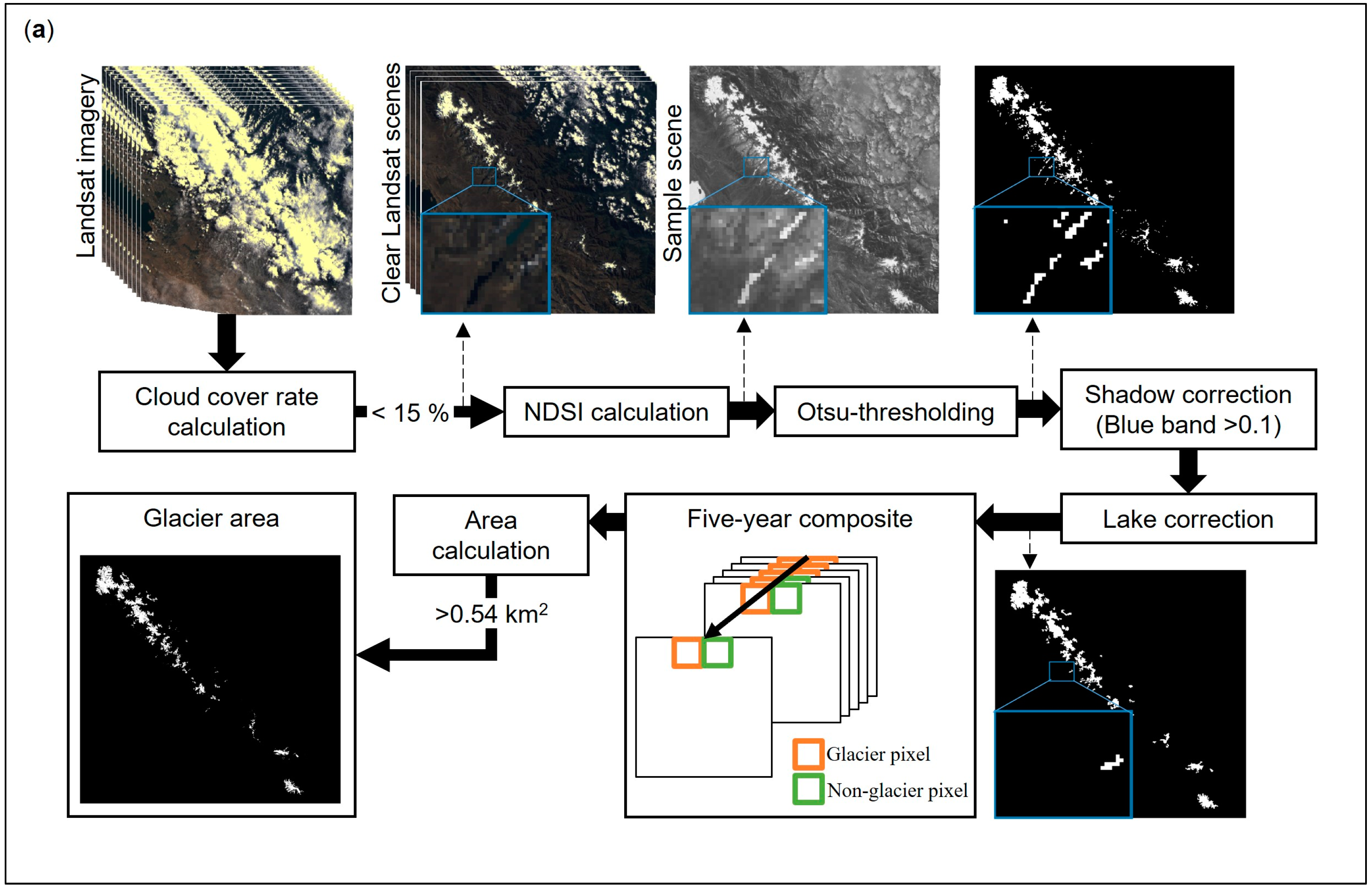
2.3.1. Glacier Mapping

To begin, Landsat 5 and Landsat 8 images free from cloud interference were carefully filtered out and utilized in glacier mapping. The NDSI for each image was calculated using the following equation:

$$\mathrm{N}\mathrm{D}\mathrm{S}\mathrm{I}=(\mathrm{G}\mathrm{r}\mathrm{e}\mathrm{e}\mathrm{n}-\mathrm{S}\mathrm{W}\mathrm{I}\mathrm{R}1)/(\mathrm{G}\mathrm{r}\mathrm{e}\mathrm{e}\mathrm{n}+\mathrm{S}\mathrm{W}\mathrm{I}\mathrm{R}1)$$

(1)

where the Green band and SWIR1 band correspond to Band 2 and Band 5, respectively, for Landsat 5, and the Green band and SWIR1 band correspond to Band 3 and Band 6, respectively, for Landsat 8.

The area within 500 m of the glaciers recorded in the GLMIS dataset was selected as the sample region for calculating the proper NDSI threshold. Unlike previous glacier mapping studies in this region, which manually selected the NDSI threshold, our study, covering a longer time period and necessitating the processing of a substantial volume of Landsat images, employed the Otsu thresholding method [38] within the sample region. This automated approach efficiently determined the optimal NDSI threshold for each Landsat image with a minimum of 0.25 and a maximum of 0.32, subsequently applied across the entire study region to delineate glacier areas.

Furthermore, a shadow cast correction was implemented using the blue band [39,40]. A TOA value below 0.1 in the blue band was considered indicative of shadow presence. Additionally, the regions identified as lakes in the subsequent section were omitted from the glacier mapping.

To minimize the potential overestimation of glacier area caused by seasonal snow cover, Landsat images from 1985 to 2021 were divided into eight segments, each covering a five-year period, except for the final period from 2020 to 2021. A pixel can only be classified as a glacier pixel if it is classified as such throughout the designated time segment, as illustrated in the Five-year composite step in Figure 2a. If a pixel was once identified as a non-glacier pixel (green pixel) during the 5-year stack, the pixel will be identified as a non-glacier pixel. Subsequently, the area of each glacier fragment was calculated. Fragments smaller than 5400 m² (equivalent to 6 Landsat pixels) were excluded following previous research [19,41], as these are more likely to represent snow patches. Additionally, the elevation distribution was calculated using the SRTM DEM to augment our understanding of glacier changes.

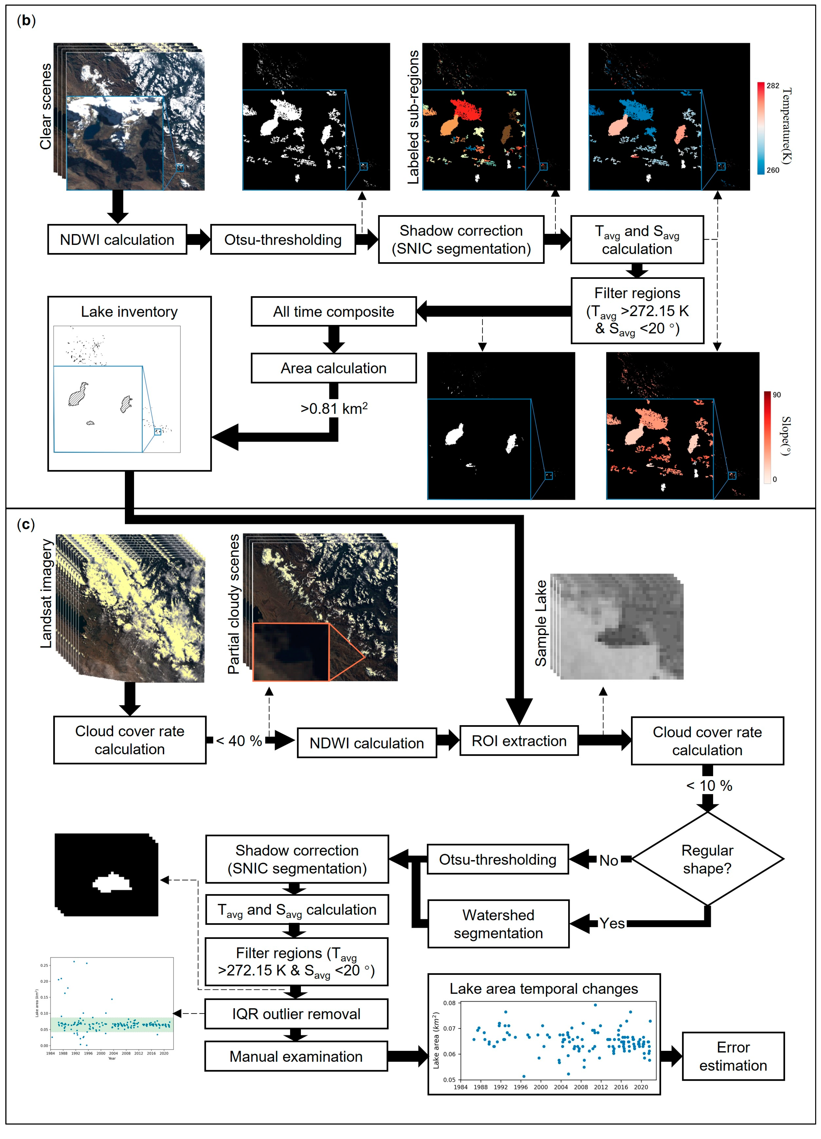
2.3.2. Glacial Lake Inventory

This study used NDWI, a commonly used index in mountainous regions like the Himalayas [42,43,44] and Andes [7] for mapping glacial lakes. This index not only enhances the identification of water surfaces but also reduces the impact of soil and terrestrial vegetation properties [23]. The NDWI is defined as follows:

$$\mathrm{N}\mathrm{D}\mathrm{W}\mathrm{I}=(\mathrm{G}\mathrm{r}\mathrm{e}\mathrm{e}\mathrm{n}-\mathrm{N}\mathrm{I}\mathrm{R})/(\mathrm{G}\mathrm{r}\mathrm{e}\mathrm{e}\mathrm{n}+\mathrm{N}\mathrm{I}\mathrm{R})$$

(2)

For Landsat 5, the Green band and NIR band correspond to Band 2 and Band 3, respectively. For Landsat 8, the Green band and NIR band correspond to Band 3 and Band 4, respectively.

Similar to the glacier mapping process, the sample region for determining the suitable NDWI threshold using the Otsu method was selected within 150 m of the waterbodies’ edge (excluding cloud pixels and those with a slope higher than 30°) in the SRTM WBD of each Landsat image. To account for potential errors from glaciers and mountain shadows, 0.1 was added to the calculated Otsu threshold, which was then applied to the entire study region in order to extract waterbodies.

In Figure 2b, the misidentified area caused by glaciers and mountain shadows is still included even after the Otsu-thresholding step. To further reduce errors attributed to glaciers and mountain shadows, a simple non-iterative clustering (SNIC) segmentation [45] was used for each waterbody identified in the Otsu-thresholding step. The SNIC segmentation method clusters similar pixels, using the pixel with the highest NDWI value as the water seed and the pixel with the steepest slope as the shadow seed. Each waterbody was divided into two sub-regions which are represented in different colors in Figure 2b, with criteria defining a sub-region as a waterbody if its average temperature exceeds 272.15 K [46] and its slope is under 20°. The temperature was derived from the average of two thermal bands in the Landsat image, while the slope was calculated using the SRTM DEM. Pixels residing within a waterbody in more than five images were classified as water pixels. Finally, all water pixels adhering to the eight-connected rule were united into individual objects. Following established methodologies [47,48], objects larger than 0.0081 km² (equivalent to 9 Landsat pixels) were identified as lakes and incorporated into the lake inventory after manually comparing with high-resolution satellite images from Google Earth and ESRI using QGIS 3.28.

2.3.3. Glacial Lake Delineation

While glacier mapping necessitates clear scenes across the entire study area, lake delineation primarily requires clear views over the lake area. Therefore, to maximize the utilization of Landsat images, the cloud cover threshold in the study area was adjusted to 40%. This adjustment enables the inclusion of clear portions of the images, even if some areas are partially affected by cloud cover. This approach is highly effective because lake areas tend to vary depending on the season (usually decreasing during the dry season from April to October), while glacier areas remain relatively stable over a short period. By utilizing partially cloudy images, we obtained three times more lake area data compared to utilizing only clear scenes, thereby reducing the seasonal bias. This analysis was performed on the Google Colab cloud platform to ensure a swift and efficient processing workflow for each individual lake object.

The extent of each lake object was derived from the resulting lake inventory in Section 2.3.2. The region of interest (ROI) is defined as the area extending 10 pixels from each lake object. A sample lake can be seen in Figure 2c. The cloud cover rate over the ROI was calculated, applying a 10% threshold to ensure that the lake area remains unaffected directly by cloud interference. The precise delineation of each lake employed the watershed segmentation method [49]. Utilizing the area within 3 pixels from each lake object that was mapped in Section 2.3.2, the outermost pixels were designated as background (land) seeds, while the top 12% NDWI-value pixels were marked as water seeds. This approach divides the area into water and land sections, defining the lake region delineated by watershed segmentation. Given that watershed segmentation methods might occasionally misidentify narrow parts of the lakes, potentially omitting certain portions, we compared the delineation result with high-resolution satellite images from Google Earth. If omission happens, the area of those lakes is extracted using the Otsu method. To minimize errors from glaciers and mountain shadows, the SNIC segmentation method, configured as in the previous section, was once again applied to each lake object, alongside the temperature and slope filter.

2.3.4. Post Process of Glacial Lake Area Data

Outliers (points that are out of the green parts in the Figure 2c IQR outlier removal step) identified by the IQR outlier detection method (as defined by Equations (3)–(5)) were automatically excluded from the obtained lake area data.

$$\mathrm{I}\mathrm{Q}\mathrm{R}={\mathrm{Q}}_3-{\mathrm{Q}}_1$$

(3)

$$\mathrm{O}\mathrm{u}\mathrm{t}\mathrm{l}\mathrm{i}\mathrm{e}\mathrm{r}<{\mathrm{Q}}_1-3\times \mathrm{I}\mathrm{Q}\mathrm{R}$$

(4)

$$\mathrm{O}\mathrm{u}\mathrm{t}\mathrm{l}\mathrm{i}\mathrm{e}\mathrm{r}>{\mathrm{Q}}_3+3\times \mathrm{I}\mathrm{Q}\mathrm{R}$$

(5)

where ${\mathrm{Q}}_1$ and ${\mathrm{Q}}_3$ represent the first quartile and the third quartile of the dataset, respectively.

Finally, all lake delineation results are manually reviewed and cross-checked with the RGB images from the corresponding Landsat images. In areas with glaciers, the presence of ice can obstruct the delineation of glacial lakes which were initially either entirely or partially covered by ice during their formation, occurring in areas where glaciers have retreated. However, they were not counted as lakes because they were smaller than the lake area threshold of 8100 m² at the time. For larger lakes that were sometimes partially covered by ice or snow, the boundary between lake and land cannot be observed by optical satellite because they are all beneath the ice surface. Such area data are not included in the final statistics. Out of all the area records, a small portion (4.6% of the total data, approximately 0.5% of the total lake area) was removed due to the following reasons: (1) partial coverage of the lake by snow or ice; (2) partial coverage of the lake by clouds; (3) misidentification of glaciers as lakes; or (4) difficulty in distinguishing the boundary between the lake and mountain shadows through visual assessment.

The monthly average areas of each lake were calculated from the obtained results. Consistent decline in monthly water levels and lake areas for five large lakes (Tuni, Incachaca, Milluni, Ajuankhota, and Chiarkota) in the study region were recorded by EPSAS (https://www.epsas.com.bo/web/, accessed on 9 October 2022) during the dry season. Thus, a linear decrease in the lake areas was assumed, and linear interpolation was applied to the monthly average lake areas during the dry season (from April to October). Finally, the average lake areas during the dry season were divided into the temporal divisions consistent with those used for glacier mapping.

2.3.5. Error Estimation

The error in glacier area mapping can result from various factors such as clouds and temporal snow cover. In this study, we use images with low cloud cover rates to minimize interference from clouds and composite multiple images to reduce overestimation caused by temporary snow. Nevertheless, accurately mapping glaciers remains challenging in the absence of suitable ground truth data [40]. Therefore, the uncertainties of glacier mapping in this study were determined using the equation proposed by Hanshaw and Bookhagen [50], which assumes that the error associated with area measurements follows a normal or Gaussian distribution.

$$\mathrm{E}\mathrm{r}\mathrm{r}\mathrm{o}\mathrm{r}\left(1\mathsf{\sigma }\right)=(\mathrm{P}/\mathrm{G})\ast 0.6872\ast {\mathrm{G}}^2/2$$

(6)

where P is the perimeter of glaciers, and G is the spatial resolution of the images, which in this case is 30 m. The calculated uncertainties during the study period are approximately 5%.

The accuracy of the lake area delineation results was evaluated using 11 Sentinel-2 images (

Table A3. List of Sentinel-2 images used in validation.

Date of Image Acquisition	Image ID
2016/4/27	S2A_MSIL1C_20160427T145722_N0201_R139_T19LEC_20160427T145719
2016/7/16	S2A_MSIL1C_20160716T144732_N0204_R139_T19LEC_20160716T145212
2017/6/1	S2A_MSIL1C_20170601T144731_N0205_R139_T19LEC_20170601T144737
2017/8/20	S2A_MSIL1C_20170820T144731_N0205_R139_T19LEC_20170820T145633
2017/11/8	S2A_MSIL1C_20171108T144731_N0206_R139_T19LEC_20171108T181232
2018/4/17	S2A_MSIL1C_20180417T144731_N0206_R139_T19LEC_20180417T200318
2018/7/6	S2A_MSIL1C_20180706T144731_N0206_R139_T19LEC_20180706T181524
2020/6/25	S2A_MSIL1C_20200625T144731_N0209_R139_T19LEC_20200625T181113
2021/5/11	S2A_MSIL1C_20210511T144731_N0300_R139_T19LEC_20210512T140023
2021/7/30	S2A_MSIL1C_20210730T144731_N0301_R139_T19LEC_20210730T181642
2021/10/18	S2A_MSIL1C_20211018T144731_N0301_R139_T19LEC_20211018T181804

) captured concurrently with the Landsat 8 images. A subset of 101 lakes was randomly selected from these images to ensure a representative distribution of lake sizes across the entire study region. The 10 m resolution of the Sentinel-2 images facilitated the manual delineation of water boundaries using the RGB image.

The uncertainty of our analysis was quantified using the root mean square error ($\mathrm{R}\mathrm{M}\mathrm{S}\mathrm{E}$), a statistically significant indicator of accuracy [51], represented by:

$$\mathrm{R}\mathrm{M}\mathrm{S}\mathrm{E}=\sqrt{\frac{1}{\mathrm{n}}{\sum }_{\mathrm{i}-1}^{\mathrm{n}}{({\mathrm{A}\mathrm{r}}_{\mathrm{i}}-{\mathrm{A}\mathrm{m}}_{\mathrm{i}})}^2}$$

(7)

where, ${\mathrm{A}\mathrm{r}}_{\mathrm{i}}$ and ${\mathrm{A}\mathrm{m}}_{\mathrm{i}}$ are the area (km²) of the ith lake derived from the Sentinel-2 RGB image and the proposed method, respectively, and n is the number of sampled lakes (=101).

Bias, the difference between the reference area ($\mathrm{A}\mathrm{r}$) and the measured area ($\mathrm{A}\mathrm{m}$), was calculated. Additionally, the misclassified area ($\mathrm{M}$), total underestimated area ($\mathrm{U}$), and total overestimated area ($\mathrm{O}$) were calculated as percentages relative to the total reference area using the following equations:

$$\mathrm{B}\mathrm{i}\mathrm{a}\mathrm{s}=\mathrm{A}\mathrm{r}-\mathrm{A}\mathrm{m}$$

(8)

$$\mathrm{M}\left(\mathrm{\%}\right)=\frac{{\sum }_1^{\mathrm{n}}\mathrm{A}\mathrm{b}\mathrm{s}\left(\mathrm{B}\mathrm{i}\mathrm{a}\mathrm{s}\right)}{{\sum }_1^{\mathrm{n}}{\mathrm{A}\mathrm{r}}_{\mathrm{i}}}\times 100$$

(9)

$$\mathrm{U}\left(\mathrm{\%}\right)=\frac{\sum \mathrm{P}\mathrm{o}\mathrm{s}\mathrm{i}\mathrm{t}\mathrm{i}\mathrm{v}\mathrm{e}\mathrm{B}\mathrm{i}\mathrm{a}\mathrm{s}}{{\sum }_1^{\mathrm{n}}{\mathrm{A}\mathrm{r}}_{\mathrm{i}}}\times 100$$

(10)

$$\mathrm{O}\left(\mathrm{\%}\right)=\frac{\sum \mathrm{A}\mathrm{b}\mathrm{s}\left(\mathrm{N}\mathrm{e}\mathrm{g}\mathrm{a}\mathrm{t}\mathrm{i}\mathrm{v}\mathrm{e}\mathrm{B}\mathrm{i}\mathrm{a}\mathrm{s}\right)}{{\sum }_1^{\mathrm{n}}{\mathrm{A}\mathrm{r}}_{\mathrm{i}}}\times 100$$

(11)

From the randomly selected lakes covering a total area of 10.6931 km², the RMSE between the proposed method and the Sentinel-2-derived area is 0.008182 km².The bias is 2.75%, with an underestimated area of 0.16% and an overestimated area of 2.59%

3. Results

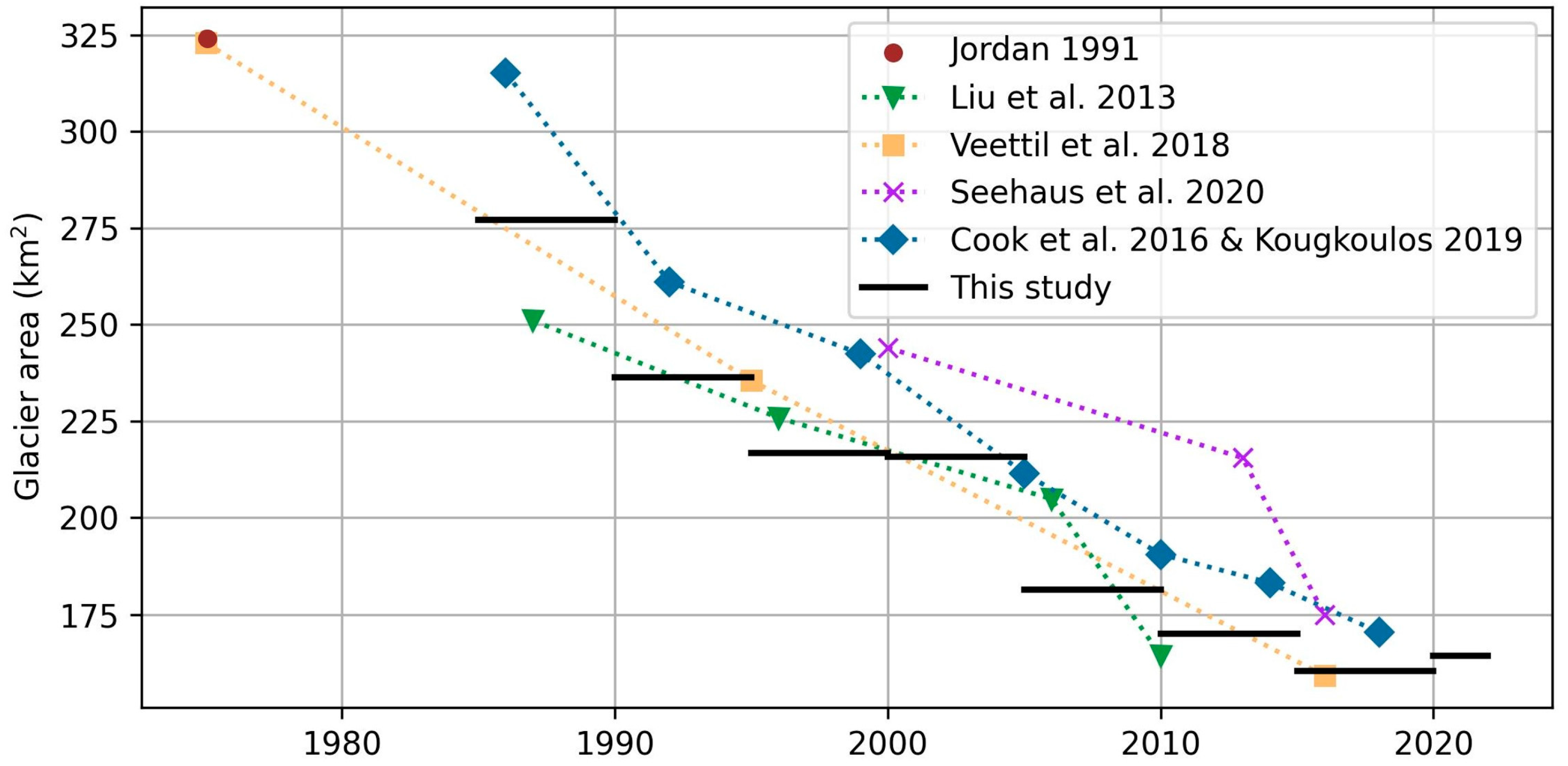
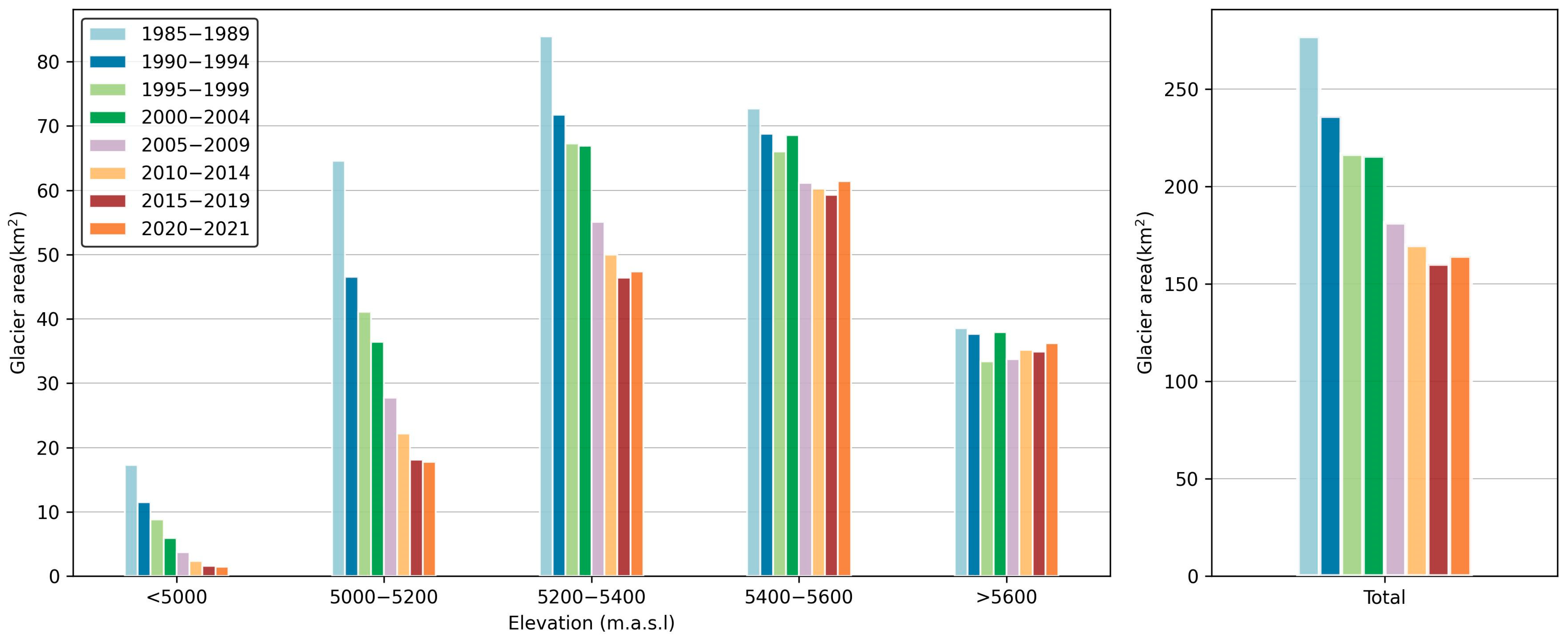
3.1. The Area Changes of Glaciers

As illustrated in Figure 3, the glacier area was 277.17 km² in 1985–1989. Over subsequent years, it experienced a significant loss, decreasing by 42% by 2021. The rate of recession was not consistent throughout the study period, with the fastest recession occurring between 1985–1989 and 1990–1994 when the glaciers diminished at a rate of 8.19 km²/year. From 2000 to 2009, the glaciers continued retreating at a high reduction rate of 6.86 km²/year. However, after 2010, the decrease notably slowed down. In the most recent period, 2020–2021, the total glacier area measured 164.33 km², nearly the same as the area in 2015–2019, which was 160.32 km². It is worth noting that all available satellite images during 2020–2021 were taken before August, which might lead to a slight overestimation of glacier area due to the temporal snow cover at the beginning of the dry season.

As predicted in previous research [5], an assessment based on elevation reveals that the most vulnerable glaciers are those situated below 5400 m.a.s.l. The most severe area loss is observed in relatively lower elevations, with glaciers below 5000 m.a.s.l. nearly disappearing. Notably, 73.9% of the area loss occurred within the 5000–5400 m range, while only 2.1% of the loss occurred above 5600 m. Glaciers below 5200 m exhibit a continuous decrease over time, especially those between 5000 and 5200 m.a.s.l. After a sharp decrease before 1990, the glaciers in this elevation range lost around 2–4% of their area per year until 2019, leaving only 17.79 km², around one-fourth of their area from 1985–1989. Glaciers between 5200 and 5400 m.a.s.l. also show a continuous downward trend since 1985, except for a slight increase observed during 2020–2021. Generally, glaciers at higher elevations experienced comparatively less area loss during the same period than those at lower elevations. Furthermore, glaciers above 5400 m.a.s.l. experienced slight area increases, particularly in 2000–2004 and 2020–2021, resulting in a higher average elevation for the remaining glaciers. In the latest period, 2020–2021, 59.4% of the glaciers were above 5400 m.a.s.l.

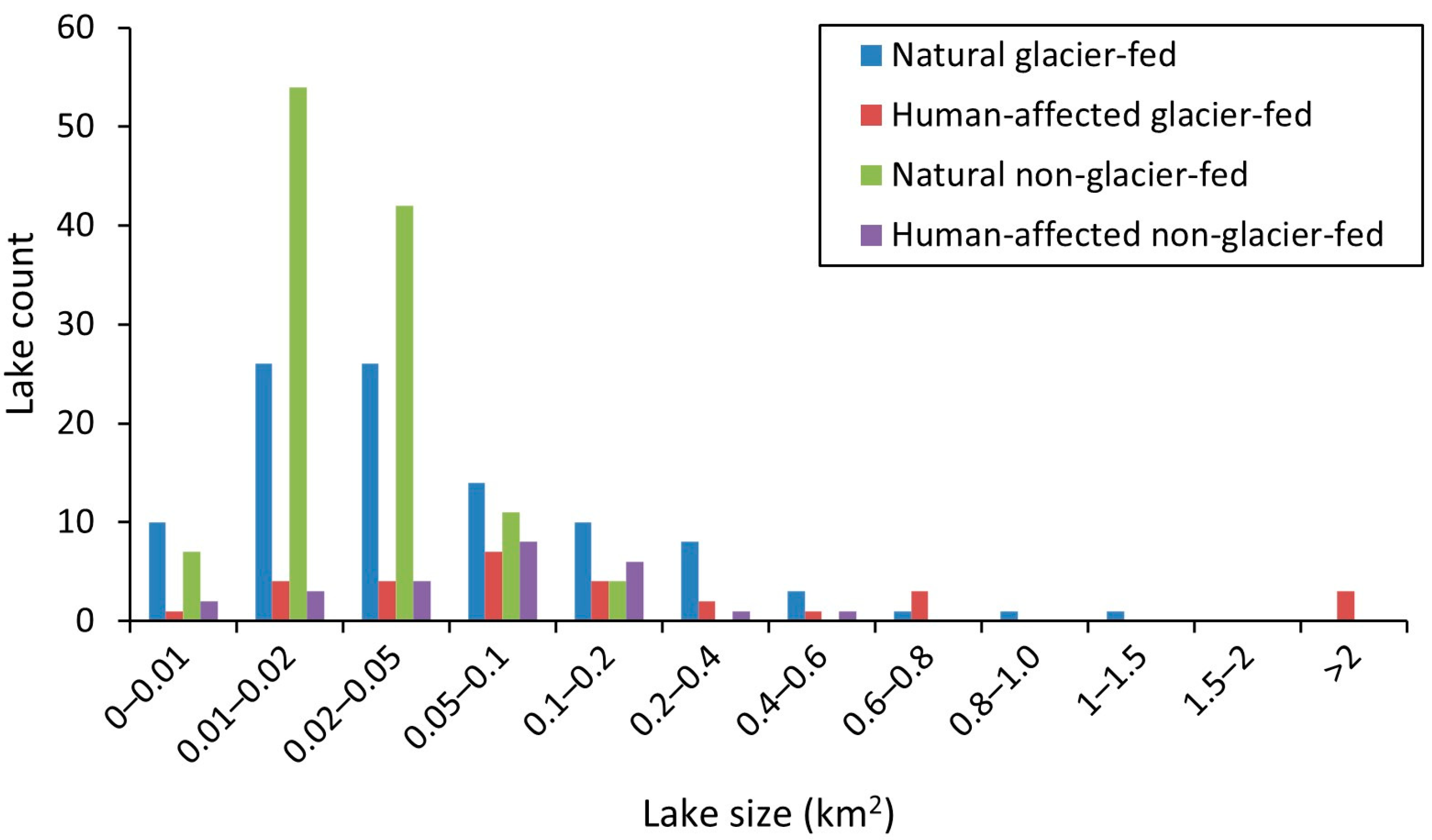
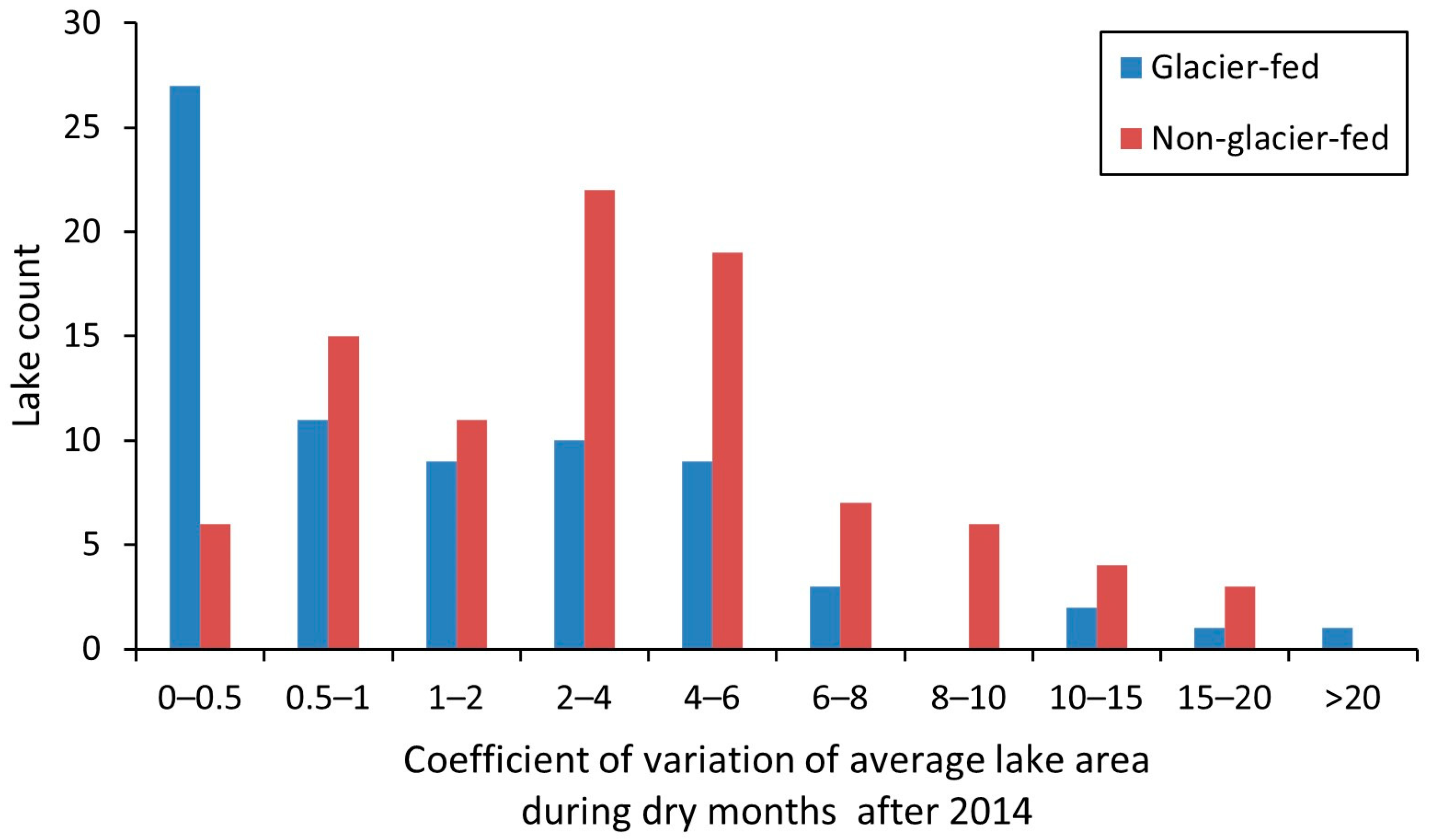
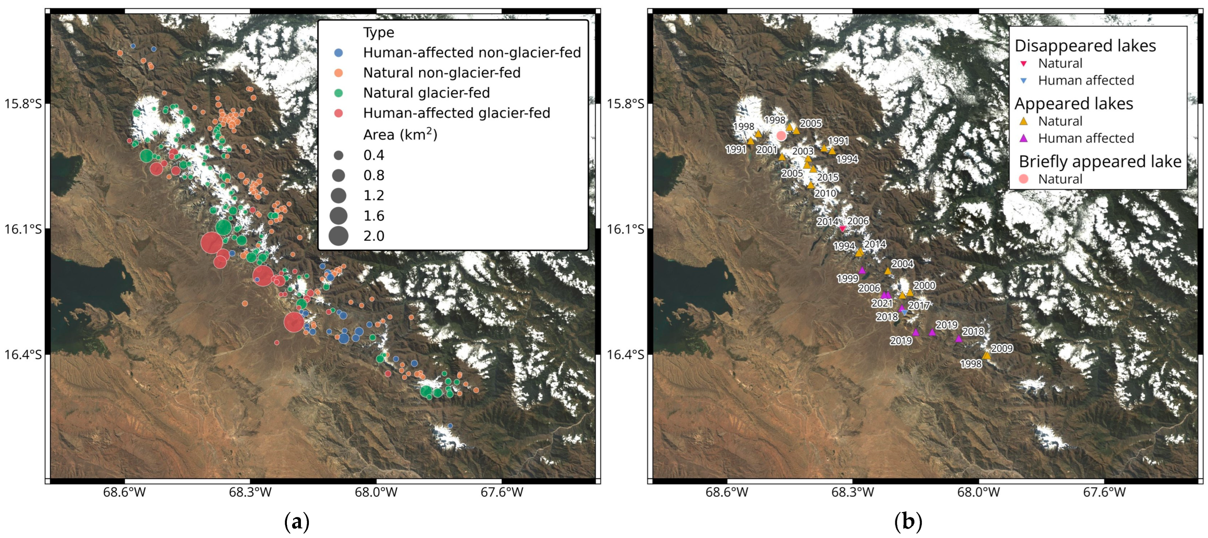
3.2. Lake Inventory and Its Spatiotemporal Distribution Characteristics

This study delivered a comprehensive inventory of lakes situated above 4300 m.a.s.l. Within the study region, a total of 272 lakes were identified. Figure 4a displays the average area of each lake during the study period, with over two-thirds of the lakes being smaller than 0.05 km² in size. The lakes were categorized into four types based on their dependency on glaciers and direct human influences (reservoir construction). This classification resulted in 100 natural glacier-fed lakes, 118 natural non-glacier-fed lakes, 29 human-affected glacier-fed lakes, and 25 human-affected non-glacier-fed lakes. Their average areas during the study period were found to be 9.92, 3.47, 11.34, and 2.34 km², respectively, indicating a tendency for glacier-fed lakes to be larger in size, potentially containing greater water volumes. The detailed lake size (dry season average area during the study period) and elevation distribution of the four categories of lakes are shown in Figure A1 and Figure A2. While higher elevation zones (above 5000 m.a.s.l.) are home to a considerable number of natural glacier-fed lakes, most human-affected lakes are limited to elevation zones below 4800 m.a.s.l. and nearly 20 human-affected lakes, including glacier-fed and non-glacier-fed ones, are located within 20 km of La Paz, Bolivia’s capital city. The storage capacity of glacier-fed and non-glacier-fed lakes is likely to have been augmented effectively by human influences to serve as water reservoirs for urban water supply and hydropower generation (Figure A2).

Over the study period, 25 lakes appeared, 3 disappeared, and 1 briefly emerged from 1990 to 2010 (Figure 4b). Naturally occurring lakes were predominantly located in the northern part of the Cordillera Real, often adjacent to retreating glacier edges. No new lakes formed without glacier feeding or human intervention. Out of the 25 appearing lakes, 22 are fed by glaciers, of which 4 are human-built reservoirs, and 18 lakes that are not intervened by humans are all located in the glacier retreated area. Three human-built, non-glacier-fed lakes (Embalse Represa de Chacaltaya, Embalse Represa Alpaquita, and Embalse Represa Hampaturi Alto), appeared during 2018–2019. Among 20 lakes appearing before 2015, only 2 were human-built reservoirs. Subsequent lakes emerging after 2016 were human-built reservoirs in the southern part of the Cordillera Real, primarily intended to supply water to nearby major cities. Of the three disappearing lakes, one was drained due to human activities, while the other two, fed by glaciers, naturally vanished, which could be a result of the declining net freshwater inflow or sedimentation. The briefly appearing lake followed a similar pattern of lakes being glacier-fed and naturally disappearing.

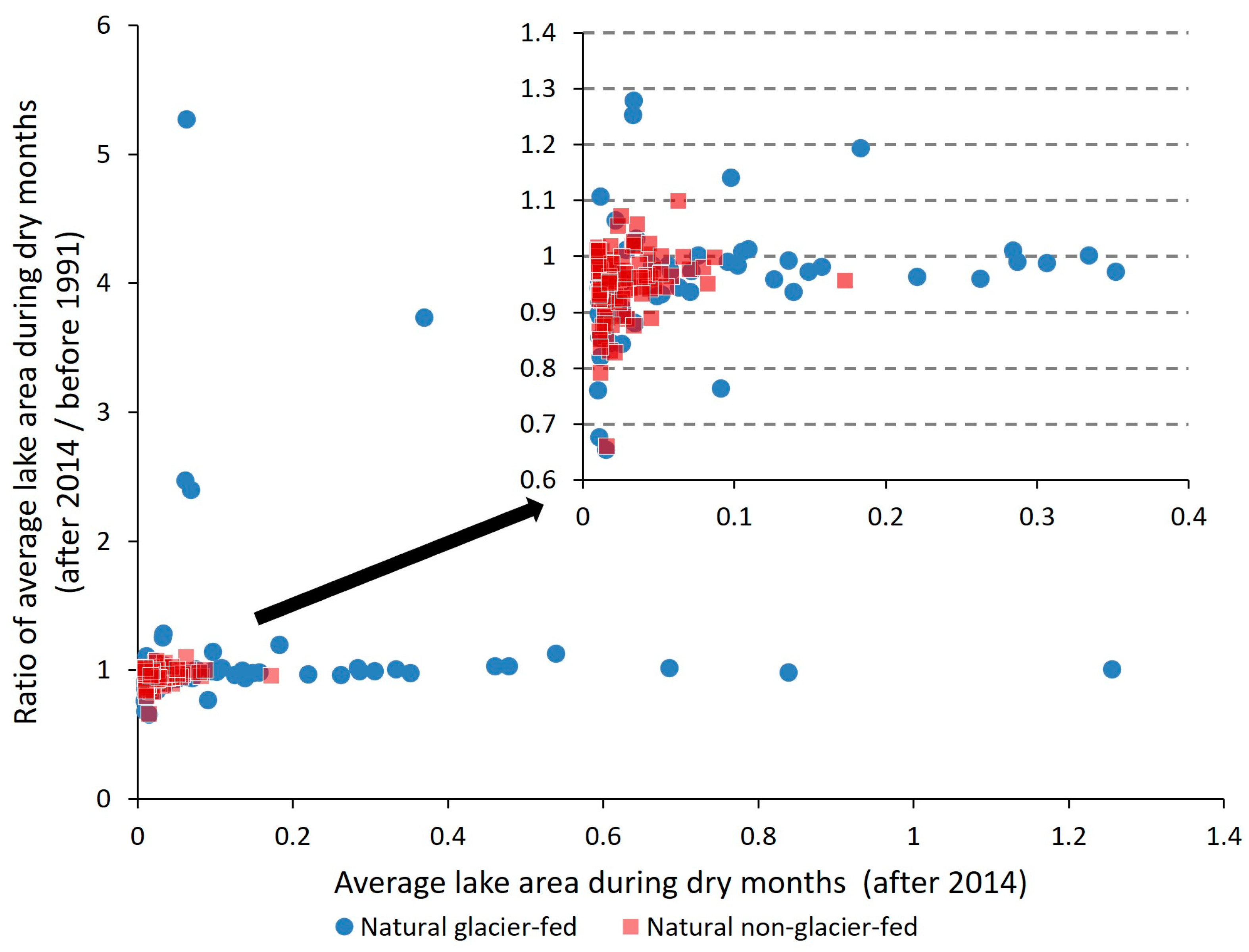
3.3. The Area Change of Lakes in Four Types

The total lake area in the study region (Figure 5) has steadily increased throughout the study period, with notable expansions during 1985–1994 and 2015–2021. Lakes receiving glacier meltwater, whether natural or human-affected, have shown varying growth patterns. Natural glacier-fed lakes showed continuous growth until 2014, expanding by 10.8% from 1985–1989 to 2010–2014. However, the lake area stabilized at approximately 10.3 km² after 2010, showing no further increase since then. Human-affected glacier-fed lakes demonstrated a consistent upward trend over the years, except for slight decreases of less than 0.1 km² in 1995–1999 and 2005–2009, with notably accelerated growth post-2005, increasing by 0.87 km². Similarly, human-affected non-glacier-fed lakes also exhibit an upward trend, with significant expansion during 1985−1999 and 2010−2021. A considerable area increase of around 0.55 km² during 2015–2021 aligns with the construction of three new water reservoirs (0.55 km²) in 2018–2019. In contrast, natural non-glacier-fed lakes remained almost unchanged. Apart from a minor increase during 1990–1994, their area remained largely unchanged, fluctuating within 5%.

To better understand the area change of each natural lake, the average lake area during dry months (May to September) for the period after 2014 and that before 1991 are compared.

It is evident from Figure 6 that the size of lakes decreased in most non-glacier-fed lakes, while there are more glacier-fed lakes that experienced an increase in area. Excluding newly formed lakes, those with an area greater than 0.03 km² before 1991 contributed nearly 85% of the remaining area growth in glacier-fed lakes. Lakes smaller than approximately 0.01 km² show a similar size distribution between glacier-fed and non-glacier-fed lakes. The total area for each type is significantly dominated by the top 40% of lakes.

Figure 7 shows the ratio of the average lake area after 2014 to that before 1991 (y axis) compared against average area after 2014 (x axis). Lakes less than 0.01 km² were excluded considering detection errors. Also, for both periods before 1994 and after 2014, lakes for which the monthly average value could not be obtained for even one month are excluded from calculating the lake area ratio.

Non-glacier-fed lakes tend to show a ratio less than 1, especially for lakes smaller than 0.05 km². Glacier-fed lakes experienced less change in lake area and a limited number of lakes show a ratio of less than 1.0, while a certain number of lakes exhibit large expansion (11 glacier-fed lakes show a ratio larger than 1.1).

The coefficient of variation (CV) of the mean monthly lake area during the dry months after 2014, calculated as the standard deviation of the mean monthly lake area divided by the mean monthly lake area, is determined for natural lakes. The histogram of CV for natural lakes indicates that non-glacier-fed lakes have a relatively higher CV, while many glacier-fed lakes show low values of CV (Figure A3). This result suggests that non-glacier-fed lakes are more susceptible to climate variability, leading to seasonal and inter-annual variations of inflow to the lake. The stability of inflow to glacier-fed lakes is reflected in their limited change in lake area, primarily due to smaller coefficients of variation in lake area (Figure 7 and Figure A3).

4. Discussion

4.1. Temporal Changes of Glaciers and Lakes

Tropical glaciers have been experiencing rapid shrinkage throughout the past decade, with this study observing over a 40% loss in glacier area within the Cordillera Real from 1985 to 2021. Studies confirm that the glacier retreat follows a non-uniform trend over time [15], strongly linked to rising air temperature [5].

Under the influence of global warming, it is predicted that glacier recession in the tropical Andes will persist [52], possibly leading to complete disappearance in mid-2050s under the RCP8.5 scenario [53]. However, research suggests that unlike glaciers in the inner tropics, which are notably susceptible to impending warming, glaciers in the drier outer tropics may exhibit greater resilience [18]. In the Cordillera Real, except for the very early study by Jorden [28] which used geodetic methods on aerial photographs, all other studies employed optical satellite images with manually selected thresholds. Liu et al. [12] applied the band ratio between the near-infrared band and shortwave infrared band, while Cook et al. [7] and Kougkoulos [11] used the band ratio between the red band and shortwave infra-red band. Vettile et al. [16] employed the NDSI method. Seehaus et al. [13] combined the band ratio method and NDSI method. Figure 8 depicts a significant loss in glacier surface area during the study period, consistent with previous research [7,11,12,13,15]. However, our latest glacier mapping results reveal a notable decline in the rate of glacier recession over the last ten years. This reduction in glacier melting is believed to be a consequence of the altered distribution of glaciers concerning elevation. Assuming an estimated temperature sensitivity of the ELA at 150 ± 30 m °C⁻¹ by Lejeune [54] and extrapolating Zongo glacier’s characteristics to the entire Cordillera Real, the rise in ELA due to recent temperature increases in the last 15 years is anticipated to be less than 100 m. Consequently, approximately 75% of current glaciers are located above 5300 m.a.s.l., the elevation where ELA is positioned. This insight may explain the observed process of glacier melting over recent decades.

Apart from precipitation and evaporation, glacier runoff stands out as a crucial factor contributing significantly to the storage of glacial lakes [55]. The area of each lake serves as a direct indicator of their water storage capacity. Rapid melting of glaciers has supported the occurrence and growth of glacial lakes [56].

In this study, several measurements and a careful validation process were carried out to map lakes comprehensively. To avoid missing newly formed lakes, especially those located in previous glacier regions with higher slopes, we carefully selected a slope threshold of 20°, which is higher than commonly used thresholds like 10° or 15°. Additionally, the slope was calculated for the entire lake object instead of a single pixel, further reducing the possibility of erroneously removing lakes. Manual visual inspections were conducted using high-resolution satellite images from Google Earth and ESRI to ensure that no such lakes were overlooked in the study region.

Although our study has detected a persistent increase in water surface area, the exclusion of human activity factors reveals the stable trend of natural glacier-fed lake area since 2010, which corresponds to the deceleration of glacier melting during the same period. Furthermore, no new naturally formed glacier-fed lakes have been found since 2015,⁰⁰ while human activities have increasingly influenced the emergence of new lakes, reflecting the regional water resources development policies. Among the 25 new lakes that appeared during the study period, those appearing after 2015 were exclusively human-built water reservoirs primarily serving nearby major cities in the southern Cordillera Real. These human-built reservoirs accounted for a water surface area 1.13 times larger than naturally occurring lakes.

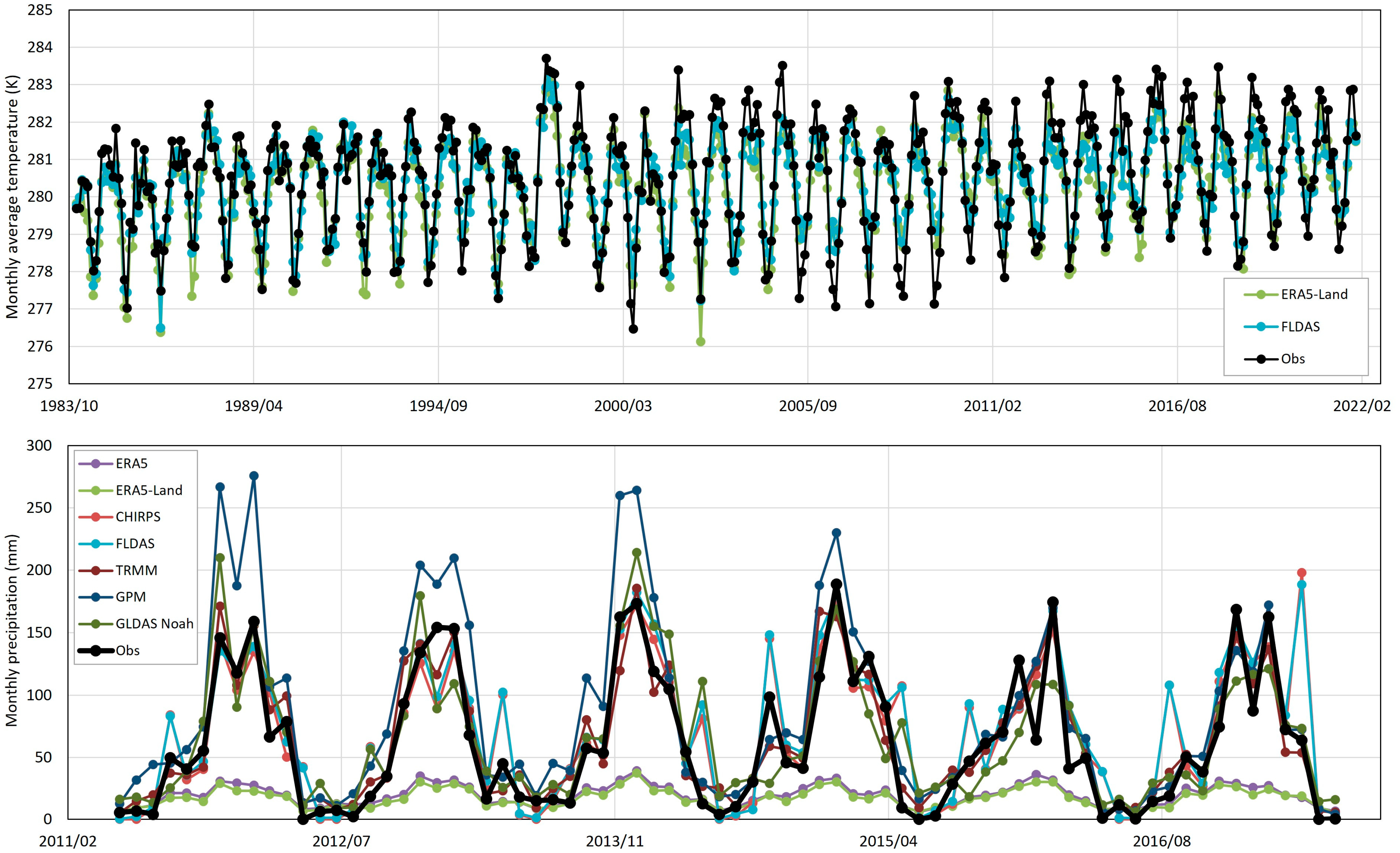
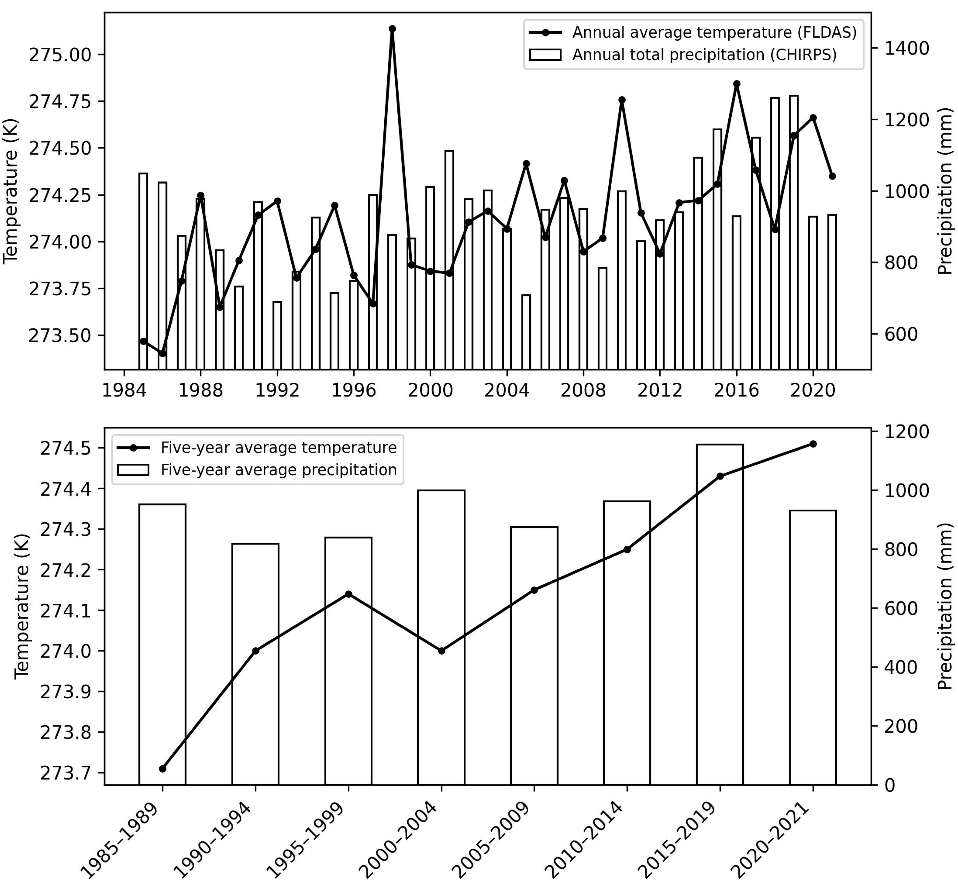
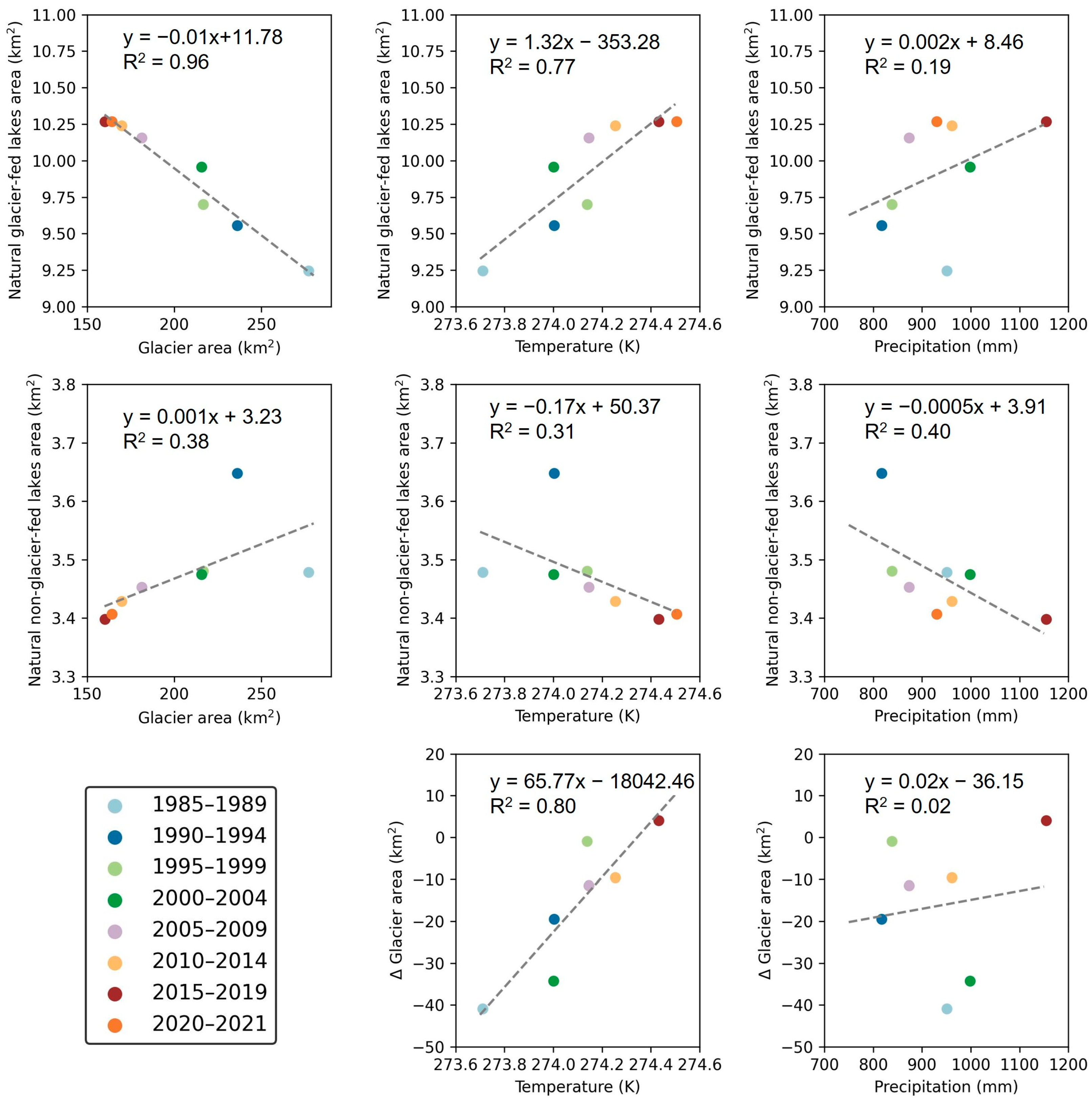
4.2. The Impact of Temperature and Precipitation on Glacier and Glacial Lakes

Temperature and precipitation play a pivotal role in glacier melting. To understand their influence on the long-term changes in glacier and glacier lake area (and volume), we compared our results of glaciers and glacier lakes with air temperature and precipitation within the study area. The area-averaged values of annual mean temperature and total precipitation for the study region were calculated for each hydrological year, i.e., from September in the preceding year to August in the present year, based on FLDAS (Famine Early Warning Systems Network (FEWS NET) Land Data Assimilation System) [57] and CHIRPS (Climate Hazards Group InfraRed Precipitation with Station Data Version 2.0 Final) [58] datasets. Based on the comparison with the observed data from specific sites, FLDAS and CHIRPS datasets were selected across various global datasets (Appendix C).

Based on FLDAS (Figure 9), the yearly average temperature is typically around 274.1 K (0.95 °C), and an increasing trend can be seen, with notably higher temperatures observed in 1998, 2010, 2016, and 2019–2020. Torres-Batllóand Martí-Cardona [59] also validated the CHIRPS precipitation dataset in the study region, observing a rise in precipitation during 1981–2018. According to CHIRPS, the yearly total precipitation is usually between 800 mm and 1000 mm. The lowest precipitation was recorded in 1992 and 2005, while relatively higher precipitation can be observed in recent years except for 2009, and the highest precipitation occurred from 2018 to 2019.

Rising temperatures play an essential part in accelerating the melting of glaciers [60]. This warming effect is particularly evident at lower elevations, where precipitation falls as rain under relatively high temperatures at low altitudes. The combination of higher temperatures and rainfall enhances the melting of glaciers [61]. In contrast to previous studies that exclusively utilized satellite images within specific years, this study has employed all the Landsat images devoid of cloud interference and short-term snow cover. Combining the glacier information at a uniform five-year interval, we have clarified the trend in glacier melting, enabling confirmation of the influence from global warming. During the period of 2015–2019, despite higher total precipitation, the glacier area decreased compared to the preceding period. This suggests a stronger impact from unprecedented high temperatures, notably in the years 2016 and 2020.

Precipitation has a mixed effect on glacier dynamics. At higher elevations or during colder periods, precipitation occurs as snowfall, contributing to glacier accumulation [62]. A notable example is the period between 2000 and 2004, characterized by lower temperatures and abundant precipitation, resulting in increased or almost stable glacier area above 5200 m.a.s.l. However, glaciers at lower elevations continued their decreasing trend, underscoring the complex interplay between temperature and precipitation in affecting the dynamics of glaciers at different elevations.

Rising temperatures directly escalate lake evaporation, while precipitation augments lake inflow, providing direct water resources. This is particularly evident in non-glacier-fed lakes unaffected by human water management (Figure 5). The total area of these lakes remained nearly constant throughout the study period, even post-2015 when precipitation surpassed the levels of previous years. The heightened evaporation due to the warming climate is likely the underlying cause.

With the anticipated increase in precipitation (CMIP5 [63]), along with the resilience of remaining glaciers at higher elevations, the deceleration in glacier melting shall continue. However, temperature will continue to be the predominant factor, with ongoing global warming, glaciers are inevitably destined to melt further.

4.3. The Inherent Connection between Glacier Melting and Lake Area under the Changing Climate

Glacial erosion creates deep depressions or overdeepenings in the landscape as glaciers move and carve through the underlying bedrock. When glaciers retreat or melt, these depressions may become filled with water, forming glacial lakes. Sediment accumulation, which includes rocks, gravel, sand, and clay carried by glaciers, can also contribute to the formation of natural barriers or dams that trap water in these depressions. During the research period, the formation of 18 natural glacial lakes was observed, all of which were located in areas where glaciers have retreated, indicating the contribution of glacial erosion as well as sedimentation. However, the sustainable formation of glacial lakes is not solely dependent on these processes. Factors such as meltwater from glaciers, inflows from precipitation and snowmelt, as well as water loss through evaporation, can all influence the size and depth of the lakes.

Glacial lakes are closely connected to the runoff from melting glaciers, contributing significantly to their water storage, and supporting lake expansion [56]. Moreover, the exacerbation of ongoing global climate change has notably fortified this correlation. In this study, to find out the inherent connection between glacier melting and lake area under the changing climate, the R² of the linear relationship between the area of the glacier, area of natural lakes, average temperature, and precipitation during the corresponding time period was calculated (Figure 10). Currently, many studies have proved that the increased precipitation intensity not only directly increases the inflow to lakes [64] but also mitigates glacier melting through snowfall by reducing surface albedo [65], thereby inhibiting the replenishment of water resources by glacial meltwater. This complex interaction between lake area and precipitation cannot be merely characterized by a positive or negative linear relationship. The anticipated increase in temperature in the Cordillera Real adds an additional layer of complexity.

Rising temperatures have led to an increase in the annual flow of glacial meltwater from glaciers to lakes [60]. In Figure 10, glacier area has shown a significant negative relationship with temperature, and the area of glaciers also shows a linear relationship with the area of natural glacier-fed lakes, with R² being as high as 0.96. As rising temperatures accelerate the melting of glaciers, the annual glacier runoff volume generally rises until it peaks. Beyond this point, runoff decreases as glaciers become unable to sustain previous meltwater volumes [66]. Consequently, rising temperatures do not consistently contribute to the expansion of lakes. The halt in natural glacial lake expansion observed in our research may serve as evidence supporting the projections made by Huss and Hock [67] in their global-scale study, indicating that Bolivian glaciers are either near or have already reached their maximum runoff. Even though lakes categorized as receiving glacier meltwater exhibit a linear correlation with temperature, R² was as high as 0.77 during the study period. Due to the diminishment of glaciers, a future temperature increase would be insufficient to yield a commensurate supply of glacial meltwater. Instead, it could promote evaporation from the lake water surface, ultimately leading to a reduction in the area of glacial lakes.

4.4. The Potential Influence on Water Resources

Changes in glacier and lake areas have potential impacts on basin water resources. However, previous studies have primarily focused on the mass balance and area changes of glaciers themselves [7,11,14]. This study proposes that the upswing in glacier melting runoff instigated by climate change significantly influences glacial lakes, offering potential water resources in the Cordillera Real.

The static nature of both the number and area of natural lakes accentuates the growing importance of water resources provided by the construction of new water reservoirs and water management infrastructures. As documented by Kinouchi et al. [8] and open map resources, many new water reservoirs and water management infrastructures were constructed in the Cordillera Real.

According to the Ministry of Environment and Water of Bolivia (MMAyA), they have invested 142 million US dollars in potable water and irrigation systems over the past decade [68]. Many international organizations have financed the construction of drinking water supply and wastewater treatment facilities in Bolivia, including the Inter-American Development Bank (IDB) [69], the European Investment Bank (EIB) [70], and the Development Bank of Latin America and the Caribbean (CAF) [71].

After the extreme drought period in 2015/2016, this study has identified five new lakes, all of which are human-constructed water reservoirs. However, not all of these new reservoirs were planned in response to the drought. Embalse Represa Hampaturi Alto was planned in 2014 [72] and brought online in 2017 [73], while Embalse Represa Alpaquita was proposed in 2013 [74] and was scheduled for completion in 2019 [75]. Embalse Represa de Chacaltaya was started construction in 2017 and was inaugurated in 2019 [75].

Concurrently, pre-existing lakes, those significantly influenced by human activities, exhibit a sustained increase despite the rising temperature and the reduction in glacier areas. This countertrend suggests that human water management plays a pivotal role in sustaining waterbodies in the study region. Moreover, it serves as an example of the preservation of precipitation through strategic reservoir deployment and judicious water management techniques. This interaction between anthropogenic interventions and climatic variables underscores the dynamic nature of water resources with regard to glacial recession, stating the essential role of human activities in shaping the hydrological landscape in the Cordillera Real.

5. Conclusions

The glaciers in the Cordillera Real have undergone severe loss during the study period, and the meltwater has contributed to the growth of lakes downstream. This study utilized over 200 Landsat images on the cloud platform GEE to develop a semi-automated method for detail mapping the changes of glaciers and glacial lakes. The method proposed in our study is efficient and significantly reduces manual work. Through the establishment of this semi-automated processing method, the study not only created a comprehensive lake inventory but also obtained a thorough observation of the spatiotemporal changes in lake surface areas. The study updated the glacier area data in the Cordillera Real and clarified the trend in glacier melting with a uniform five-year interval. The application of this method revealed that a significant portion of glaciers shrank before 2010, especially those situated below 5400 m.a.s.l. However, as the distribution of glaciers is more concentrated at high elevations, and thus more resilient to the rising temperature of recent years, the rate of glacier recession has slowed down in recent years. Similarly, after a consistent increase since 1985, the area of natural glacier-fed lakes stabilized after 2010. As these lakes are still receiving melting waters from glaciers, their seasonal variations are lower than lakes that are not fed by glaciers. Even though the overall area of lakes shows a continuous increase over the years, the increase almost entirely comes from the contribution of human-affected lakes.

The analysis of changes in glaciers and glacial lakes over 38 years indicated a strong influence of climate change on glacier retreat and lake expansion. These changes have increased the water resources available for future use. The method developed in this study can be further employed for future glacier and glacial lake monitoring due to its high temporal resolution, contributing to the prevention of glacial lake outburst flood disasters. The findings of this study serve as a valuable resource for assessing the impact of climate change on water resources. Future research could enhance observation by incorporating higher-resolution satellite imagery to better evaluate the effects of glacier melting and lake evolution on local water resources and society.

References

1. Immerzeel, W.W.; Van Beek, L.P.H.; Bierkens, M.F.P. Climate Change Will Affect the Asian Water Towers. Science 2010, 328, 1382–1385. [Google Scholar] [CrossRef] [PubMed]
2. Vergara, W.; Deeb, A.; Valencia, A.; Bradley, R.; Francou, B.; Zarzar, A.; Grünwaldt, A.; Haeussling, S. Economic Impacts of Rapid Glacier Retreat in the Andes. EoS Trans. 2007, 88, 261–264. [Google Scholar] [CrossRef]
3. Kaser, G. A Review of the Modern Fluctuations of Tropical Glaciers. Glob. Planet. Change 1999, 22, 93–103. [Google Scholar] [CrossRef]
4. Zemp, M.; Huss, M.; Thibert, E.; Eckert, N.; McNabb, R.; Huber, J.; Barandun, M.; Machguth, H.; Nussbaumer, S.U.; Gärtner-Roer, I.; et al. Global Glacier Mass Changes and Their Contributions to Sea-Level Rise from 1961 to 2016. Nature 2019, 568, 382–386. [Google Scholar] [CrossRef] [PubMed]
5. Bradley, R.S.; Vuille, M.; Diaz, H.F.; Vergara, W. Threats to Water Supplies in the Tropical Andes. Science 2006, 312, 1755–1756. [Google Scholar] [CrossRef] [PubMed]
6. Rabatel, A.; Francou, B.; Soruco, A.; Gomez, J.; Cáceres, B.; Ceballos, J.L.; Basantes, R.; Vuille, M.; Sicart, J.-E.; Huggel, C.; et al. Current State of Glaciers in the Tropical Andes: A Multi-Century Perspective on Glacier Evolution and Climate Change. Cryosphere 2013, 7, 81–102. [Google Scholar] [CrossRef]
7. Cook, S.J.; Kougkoulos, I.; Edwards, L.A.; Dortch, J.; Hoffmann, D. Glacier Change and Glacial Lake Outburst Flood Risk in the Bolivian Andes. Cryosphere 2016, 10, 2399–2413. [Google Scholar] [CrossRef]
8. Carey, M. Living and Dying with Glaciers: People’s Historical Vulnerability to Avalanches and Outburst Floods in Peru. Glob. Planet. Change 2005, 47, 122–134. [Google Scholar] [CrossRef]
9. Dussaillant, I.; Berthier, E.; Brun, F.; Masiokas, M.; Hugonnet, R.; Favier, V.; Rabatel, A.; Pitte, P.; Ruiz, L. Two Decades of Glacier Mass Loss along the Andes. Nat. Geosci. 2019, 12, 802–808. [Google Scholar] [CrossRef]
10. Kinouchi, T.; Nakajima, T.; Mendoza, J.; Fuchs, P.; Asaoka, Y. Water Security in High Mountain Cities of the Andes under a Growing Population and Climate Change: A Case Study of La Paz and El Alto, Bolivia. Water Secur. 2019, 6, 100025. [Google Scholar] [CrossRef]
11. Kougkoulos, I. Glacial Lake Outburst Flood Risk in the Bolivian Andes. Ph.D. Dissertation, Manchester Metropolitan University, Manchester, UK, 2019. [Google Scholar]
12. Liu, T.; Kinouchi, T.; Ledezma, F. Characterization of Recent Glacier Decline in the Cordillera Real by LANDSAT, ALOS, and ASTER Data. Remote Sens. Environ. 2013, 137, 158–172. [Google Scholar] [CrossRef]
13. Seehaus, T.; Malz, P.; Sommer, C.; Soruco, A.; Rabatel, A.; Braun, M. Mass Balance and Area Changes of Glaciers in the Cordillera Real and Tres Cruces, Bolivia, between 2000 and 2016. J. Glaciol. 2020, 66, 124–136. [Google Scholar] [CrossRef]
14. Sicart, J.E.; Hock, R.; Ribstein, P.; Litt, M.; Ramirez, E. Analysis of Seasonal Variations in Mass Balance and Meltwater Discharge of the Tropical Zongo Glacier by Application of a Distributed Energy Balance Model. J. Geophys. Res. 2011, 116, D13105. [Google Scholar] [CrossRef]
15. Soruco, A.; Vincent, C.; Francou, B.; Gonzalez, J.F. Glacier Decline between 1963 and 2006 in the Cordillera Real, Bolivia. Geophys. Res. Lett. 2009, 36, 2008GL036238. [Google Scholar] [CrossRef]
16. Veettil, B.K.; Wang, S.; Simões, J.C.; Pereira, S.F.R. Glacier Monitoring in the Eastern Mountain Ranges of Bolivia from 1975 to 2016 Using Landsat and Sentinel-2 Data. Environ. Earth Sci. 2018, 77, 452. [Google Scholar] [CrossRef]
17. Veettil, B.K.; Kamp, U. Glacial Lakes in the Andes under a Changing Climate: A Review. J. Earth Sci. 2021, 32, 1575–1593. [Google Scholar] [CrossRef]
18. Vuille, M.; Carey, M.; Huggel, C.; Buytaert, W.; Rabatel, A.; Jacobsen, D.; Soruco, A.; Villacis, M.; Yarleque, C.; Elison Timm, O.; et al. Rapid Decline of Snow and Ice in the Tropical Andes—Impacts, Uncertainties and Challenges Ahead. Earth Sci. Rev. 2018, 176, 195–213. [Google Scholar] [CrossRef]
19. Drenkhan, F.; Guardamino, L.; Huggel, C.; Frey, H. Current and Future Glacier and Lake Assessment in the Deglaciating Vilcanota-Urubamba Basin, Peruvian Andes. Glob. Planet. Change 2018, 169, 105–118. [Google Scholar] [CrossRef]
20. Song, C.; Sheng, Y. Contrasting Evolution Patterns between Glacier-Fed and Non-Glacier-Fed Lakes in the Tanggula Mountains and Climate Cause Analysis. Clim. Change 2016, 135, 493–507. [Google Scholar] [CrossRef]
21. Paul, F.; Kääb, A.; Maisch, M.; Kellenberger, T.; Haeberli, W. The New Remote-Sensing-Derived Swiss Glacier Inventory: I. Methods. Ann. Glaciol. 2002, 34, 355–361. [Google Scholar] [CrossRef]
22. Hall, D.K.; Riggs, G.A.; Salomonson, V.V.; DiGirolamo, N.E.; Bayr, K.J. MODIS Snow-Cover Products. Remote Sens. Environ. 2002, 83, 181–194. [Google Scholar] [CrossRef]
23. McFEETERS, S.K. The Use of the Normalized Difference Water Index (NDWI) in the Delineation of Open Water Features. Int. J. Remote Sens. 1996, 17, 1425–1432. [Google Scholar] [CrossRef]
24. Pekel, J.-F.; Cottam, A.; Gorelick, N.; Belward, A.S. High-Resolution Mapping of Global Surface Water and Its Long-Term Changes. Nature 2016, 540, 418–422. [Google Scholar] [CrossRef] [PubMed]
25. Veh, G.; Korup, O.; Roessner, S.; Walz, A. Detecting Himalayan Glacial Lake Outburst Floods from Landsat Time Series. Remote Sens. Environ. 2018, 207, 84–97. [Google Scholar] [CrossRef]
26. Zhao, H.; Chen, F.; Zhang, M. A Systematic Extraction Approach for Mapping Glacial Lakes in High Mountain Regions of Asia. IEEE J. Sel. Top. Appl. Earth Obs. Remote Sens. 2018, 11, 2788–2799. [Google Scholar] [CrossRef]
27. Paul, F.; Rastner, P. Glacier Extents in Peru and Bolivia Are Overestimated in RGIv6 by 27%. In Proceedings of the EGU General Assembly 2023, Vienna, Austria, 24–28 April 2023. EGU23-12724. [Google Scholar] [CrossRef]
28. Jordan, E. Die Gletscher der Bolivianischen Anden: Eine Photogrammetrisch-Kartographische Bestandsaufnahme der Gletscher Boliviens Als Grundlage für Klimatische Deutungen und Potential für die Wirtschaftliche Nutzung; Steiner: Stuttgart, Germany, 1991; ISBN 978-3-515-04917-7. [Google Scholar]
29. Rabatel, A.; Jomelli, V.; Naveau, P.; Francou, B.; Grancher, D. Dating of Little Ice Age Glacier Fluctuations in the Tropical Andes: Charquini Glaciers, Bolivia, 16°S. Comptes Rendus. Géoscience 2005, 337, 1311–1322. [Google Scholar] [CrossRef]
30. Raup, B.; Racoviteanu, A.; Khalsa, S.J.S.; Helm, C.; Armstrong, R.; Arnaud, Y. The GLIMS Geospatial Glacier Database: A New Tool for Studying Glacier Change. Glob. Planet. Change 2007, 56, 101–110. [Google Scholar] [CrossRef]
31. Jomelli, V.; Favier, V.; Rabatel, A.; Brunstein, D.; Hoffmann, G.; Francou, B. Fluctuations of Glaciers in the Tropical Andes over the Last Millennium and Palaeoclimatic Implications: A Review. Palaeogeogr. Palaeoclimatol. Palaeoecol. 2009, 281, 269–282. [Google Scholar] [CrossRef]
32. Rabatel, A.; Bermejo, A.; Loarte, E.; Soruco, A.; Gomez, J.; Leonardini, G.; Vincent, C.; Sicart, J.E. Can the Snowline Be Used as an Indicator of the Equilibrium Line and Mass Balance for Glaciers in the Outer Tropics? J. Glaciol. 2012, 58, 1027–1036. [Google Scholar] [CrossRef]
33. Yao, X.; Liu, S.; Han, L.; Sun, M.; Zhao, L. Definition and Classification System of Glacial Lake for Inventory and Hazards Study. J. Geogr. Sci. 2018, 28, 193–205. [Google Scholar] [CrossRef]
34. Foga, S.; Scaramuzza, P.L.; Guo, S.; Zhu, Z.; Dilley, R.D.; Beckmann, T.; Schmidt, G.L.; Dwyer, J.L.; Joseph Hughes, M.; Laue, B. Cloud Detection Algorithm Comparison and Validation for Operational Landsat Data Products. Remote Sens. Environ. 2017, 194, 379–390. [Google Scholar] [CrossRef]
35. Farr, T.G.; Rosen, P.A.; Caro, E.; Crippen, R.; Duren, R.; Hensley, S.; Kobrick, M.; Paller, M.; Rodriguez, E.; Roth, L.; et al. The Shuttle Radar Topography Mission. Rev. Geophys. 2007, 45, 2005RG000183. [Google Scholar] [CrossRef]
36. Alvizuri-Tintaya, P.A.; Rios-Ruiz, M.; Lora-Garcia, J.; Torregrosa-López, J.I.; Lo-Iacono-Ferreira, V.G. Study and Evaluation of Surface Water Resources Affected by Ancient and Illegal Mining in the Upper Part of the Milluni Micro-Basin, Bolivia. Resources 2022, 11, 36. [Google Scholar] [CrossRef]
37. Caballero, Y.; Chevallier, P.; Gallaire, R.; Pillco, R. Flow Modelling in a High Mountain Valley Equipped with Hydropower Plants: Rio Zongo Valley, Cordillera Real, Bolivia. Hydrol. Process. 2004, 18, 939–957. [Google Scholar] [CrossRef]
38. Otsu, N. A Threshold Selection Method from Gray-Level Histograms. IEEE Trans. Syst. Man Cybern. 1979, 9, 62–66. [Google Scholar] [CrossRef]
39. Mölg, N.; Bolch, T.; Rastner, P.; Strozzi, T.; Paul, F. A Consistent Glacier Inventory for Karakoram and Pamir Derived from Landsat Data: Distribution of Debris Cover and Mapping Challenges. Earth Syst. Sci. Data 2018, 10, 1807–1827. [Google Scholar] [CrossRef]
40. Paul, F.; Andreassen, L.M.; Winsvold, S.H. A New Glacier Inventory for the Jostedalsbreen Region, Norway, from Landsat TM Scenes of 2006 and Changes since 1966. Ann. Glaciol. 2011, 52, 153–162. [Google Scholar] [CrossRef]
41. Bolch, T.; Menounos, B.; Wheate, R. Landsat-Based Inventory of Glaciers in Western Canada, 1985–2005. Remote Sens. Environ. 2010, 114, 127–137. [Google Scholar] [CrossRef]
42. Wang, X.; Guo, X.; Yang, C.; Liu, Q.; Wei, J.; Zhang, Y.; Liu, S.; Zhang, Y.; Jiang, Z.; Tang, Z. Glacial Lake Inventory of High-Mountain Asia in 1990 and 2018 Derived from Landsat Images. Earth Syst. Sci. Data 2020, 12, 2169–2182. [Google Scholar] [CrossRef]
43. Jiang, S.; Nie, Y.; Liu, Q.; Wang, J.; Liu, L.; Hassan, J.; Liu, X.; Xu, X. Glacier Change, Supraglacial Debris Expansion and Glacial Lake Evolution in the Gyirong River Basin, Central Himalayas, between 1988 and 2015. Remote Sens. 2018, 10, 986. [Google Scholar] [CrossRef]
44. Li, J.; Sheng, Y. An Automated Scheme for Glacial Lake Dynamics Mapping Using Landsat Imagery and Digital Elevation Models: A Case Study in the Himalayas. Int. J. Remote Sens. 2012, 33, 5194–5213. [Google Scholar] [CrossRef]
45. Achanta, R.; Susstrunk, S. Superpixels and Polygons Using Simple Non-Iterative Clustering. In Proceedings of the 2017 IEEE Conference on Computer Vision and Pattern Recognition (CVPR), Honolulu, HI, USA, 21–26 July 2017; pp. 4895–4904. [Google Scholar]
46. Shugar, D.H.; Burr, A.; Haritashya, U.K.; Kargel, J.S.; Watson, C.S.; Kennedy, M.C.; Bevington, A.R.; Betts, R.A.; Harrison, S.; Strattman, K. Rapid Worldwide Growth of Glacial Lakes since 1990. Nat. Clim. Change 2020, 10, 939–945. [Google Scholar] [CrossRef]
47. Mitkari, K.V.; Arora, M.K.; Tiwari, R.K. Extraction of Glacial Lakes in Gangotri Glacier Using Object-Based Image Analysis. IEEE J. Sel. Top. Appl. Earth Obs. Remote Sens. 2017, 10, 5275–5283. [Google Scholar] [CrossRef]
48. Nie, Y.; Sheng, Y.; Liu, Q.; Liu, L.; Liu, S.; Zhang, Y.; Song, C. A Regional-Scale Assessment of Himalayan Glacial Lake Changes Using Satellite Observations from 1990 to 2015. Remote Sens. Environ. 2017, 189, 1–13. [Google Scholar] [CrossRef]
49. Vincent, L.; Soille, P. Watersheds in Digital Spaces: An Efficient Algorithm Based on Immersion Simulations. IEEE Trans. Pattern Anal. Mach. Intell. 1991, 13, 583–598. [Google Scholar] [CrossRef]
50. Hanshaw, M.N.; Bookhagen, B. Glacial Areas, Lake Areas, and Snow Lines from 1975 to 2012: Status of the Cordillera Vilcanota, Including the Quelccaya Ice Cap, Northern Central Andes, Peru. Cryosphere 2014, 8, 359–376. [Google Scholar] [CrossRef]
51. Jawak, S.D.; Luis, A.J. A Semiautomatic Extraction of Antarctic Lake Features Using Worldview-2 Imagery. Photogramm. Eng. Remote Sens. 2014, 80, 939–952. [Google Scholar] [CrossRef]
52. Vuille, M.; Francou, B.; Wagnon, P.; Juen, I.; Kaser, G.; Mark, B.G.; Bradley, R.S. Climate Change and Tropical Andean Glaciers: Past, Present and Future. Earth-Sci. Rev. 2008, 89, 79–96. [Google Scholar] [CrossRef]
53. Yarleque, C.; Vuille, M.; Hardy, D.R.; Timm, O.E.; De La Cruz, J.; Ramos, H.; Rabatel, A. Projections of the Future Disappearance of the Quelccaya Ice Cap in the Central Andes. Sci. Rep. 2018, 8, 15564. [Google Scholar] [CrossRef]
54. Lejeune, Y. Apports Des Modèles de Neige CROCUS et de Sol ISBA à l’étude Du Bilan Glaciologique d’un Glacier Tropical et Du Bilan Hydrologique de Son Bassin Versant. Ph.D. Dissertation, Université Joseph-Fourier, Grenoble, France, 2009. [Google Scholar]
55. Lei, Y.; Yao, T.; Bird, B.W.; Yang, K.; Zhai, J.; Sheng, Y. Coherent Lake Growth on the Central Tibetan Plateau since the 1970s: Characterization and Attribution. J. Hydrol. 2013, 483, 61–67. [Google Scholar] [CrossRef]
56. Bajracharya, S.R.; Mool, P. Glaciers, Glacial Lakes and Glacial Lake Outburst Floods in the Mount Everest Region, Nepal. Ann. Glaciol. 2009, 50, 81–86. [Google Scholar] [CrossRef]
57. McNally, A.; NASA GSFC Hydrological Sciences Laboratory (HSL). FLDAS Noah Land Surface Model L4 Global Monthly 0.1 × 0.1 Degree (MERRA-2 and CHIRPS) V001 2018. Available online: https://developers.google.com/earth-engine/datasets/catalog/NASA_FLDAS_NOAH01_C_GL_M_V001 (accessed on 13 June 2023).
58. Funk, C.C.; Peterson, P.J.; Landsfeld, M.F.; Pedreros, D.H.; Verdin, J.P.; Rowland, J.D.; Romero, B.E.; Husak, G.J.; Michaelsen, J.C.; Verdin, A.P. A Quasi-Global Precipitation Time Series for Drought Monitoring; U.S. Geological Survey: Reston, VA, USA, 2014.
59. Torres-Batlló, J.; Martí-Cardona, B. Precipitation Trends over the Southern Andean Altiplano from 1981 to 2018. J. Hydrol. 2020, 590, 125485. [Google Scholar] [CrossRef]
60. Zhang, G.; Chen, W.; Xie, H. Tibetan Plateau’s Lake Level and Volume Changes from NASA’s ICESat/ICESat-2 and Landsat Missions. Geophys. Res. Lett. 2019, 46, 13107–13118. [Google Scholar] [CrossRef]
61. Woo, M. Consequences of Climatic Change for Hydrology in Permafrost Zones. J. Cold Reg. Eng. 1990, 4, 15–20. [Google Scholar] [CrossRef]
62. Mott, R.; Wolf, A.; Kehl, M.; Kunstmann, H.; Warscher, M.; Grünewald, T. Avalanches and Micrometeorology Driving Mass and Energy Balance of the Lowest Perennial Ice Field of the Alps: A Case Study. Cryosphere 2019, 13, 1247–1265. [Google Scholar] [CrossRef]
63. Taylor, K.E.; Stouffer, R.J.; Meehl, G.A. An Overview of CMIP5 and the Experiment Design. Bull. Am. Meteorol. Soc. 2012, 93, 485–498. [Google Scholar] [CrossRef]
64. Qiao, B.; Zhu, L. Difference and Cause Analysis of Water Storage Changes for Glacier-Fed and Non-Glacier-Fed Lakes on the Tibetan Plateau. Sci. Total Environ. 2019, 693, 133399. [Google Scholar] [CrossRef]
65. Yue, X.; Li, Z.; Li, H.; Wang, F.; Jin, S. Multi-Temporal Variations in Surface Albedo on Urumqi Glacier No.1 in Tien Shan, under Arid and Semi-Arid Environment. Remote Sens. 2022, 14, 808. [Google Scholar] [CrossRef]
66. Jansson, P.; Hock, R.; Schneider, T. The Concept of Glacier Storage: A Review. J. Hydrol. 2003, 282, 116–129. [Google Scholar] [CrossRef]
67. Huss, M.; Hock, R. Global-Scale Hydrological Response to Future Glacier Mass Loss. Nat. Clim Change 2018, 8, 135–140. [Google Scholar] [CrossRef]
68. BNamericas. Bolivia Invests in Water Projects to Ward of Drought. Available online: https://www.bnamericas.com/en/news/bolivia-invests-in-water-projects-to-ward-off-drought (accessed on 22 March 2024).
69. The Inter-American Development Bank and the Inter-American Investment Corporation. IDB Country Strategy with Bolivia (2022–2025). Available online: https://idbinvest.org/sites/default/files/2022-04/Bolivia-Country-Strategy-IDB-Group-2022.pdf (accessed on 22 March 2024).
70. European Investment Bank. Environmental and Social Data Sheet. 2017. Available online: https://www.eib.org/en/projects/all/20170789 (accessed on 22 March 2024).
71. Development Bank of Latin America and the Caribbean. CAF Approves US$240 Million to Improve Water Security in Bolivia. Available online: https://www.caf.com/en/currently/news/2024/03/caf-approves-us-240-million-to-improve-water-security-in-bolivia/ (accessed on 22 March 2024).
72. EPSAS. Hampaturi es Una Realidad. Available online: https://www.epsas.com.bo/web/wp-content/uploads/2019/01/hampaturi17.pdf (accessed on 22 March 2024).
73. BNamericas. Bolivia Moving ahead with La Paz Water Projects. Available online: https://www.bnamericas.com/en/news/bolivia-moving-ahead-with-la-paz-water-projects (accessed on 22 March 2024).
74. Buxton, N.; Escobar, M.; Purkey, D.; Lima, N. Water Scarcity, Climate Change and Bolivia: Planning for Climate Uncertainties; Discussion Brief; Stockholm Environment Institute: Stockholm, Sweden, 2013. [Google Scholar]
75. EPSAS. Audiencia Inicial Pública de Rendición de Cuentas Gestión 2017. Available online: https://www.epsas.com.bo/web/wp-content/uploads/2020/06/InformeFinal2017.pdf (accessed on 22 March 2024).
Figure 1. Study region (above 4300 m.a.s.l.). The municipalities boundary of Bolivia comes from the GADM database version 3.4, April 2018 (www.gadm.org).
Remotesensing 16 01231 g001
Figure 2. Flow chart of (a) glacier mapping, (b) lake inventory mapping, and (c) lake area change detection. (Tavg: average temperature of each sub-region; Savg: average slope of each sub-region).
Remotesensing 16 01231 g002aRemotesensing 16 01231 g002b
Figure 3. Glacier area along different elevations.
Remotesensing 16 01231 g003
Figure 4. (a) Lake classification and area; (b) appeared, disappeared, and briefly appeared lakes.
Remotesensing 16 01231 g004
Figure 5. Temporal changes in the area of (ad) each lake type and (e) all types by area classification, and (f) the total area and number of each lake type.
Remotesensing 16 01231 g005
Figure 6. Each lake area during the dry months (May to September) for the periods before 1991 and after 2014 plotted against the cumulative percentage of the number of lakes. (a) Glacier-fed lakes; (b) Non-glacier-fed Lakes. Lakes are sorted in ascending order based on their area during the period after 2014.
Remotesensing 16 01231 g006
Figure 7. The ratio of the average lake area during dry months (May to September) for the period after 2014 to that before 1991 compared against the average lake area after 2014.
Remotesensing 16 01231 g007
Figure 8. The glacier area from this study compared with previous studies [7,11,12,13,16,28].
Remotesensing 16 01231 g008
Figure 9. Temperature data from FLDAS and precipitation data from CHIRPS in the study region. Above: annual data; Below: five-year average corresponding to the period for glacier and glacial lakes analysis.
Remotesensing 16 01231 g009
Figure 10. Correlation between glacier area, natural glacier-fed and non-glacier-fed lake area, average temperature, and average yearly precipitation of the corresponding period, and correlation between glacier area change from the previous period and the temperature and precipitation.
Remotesensing 16 01231 g010