Lightweight and Stable Multi-Feature Databases for Efficient Geometric Localization of Remote Sensing Images

Abstract

The surge in remote sensing satellites and diverse imaging modes poses substantial challenges for ground systems. Swift and high-precision geolocation is the foundational requirement for subsequent remote sensing image applications. Breakthroughs in intelligent on-orbit processing now enable on-orbit geometric processing. In the absence of control data on board, a recent trend is to introduce reference data onto satellites. However, the pre-storage of traditional reference images or control point databases presents a significant challenge to the limited on-board data storage capacity. Therefore, oriented to the demand for control information acquisition during on-orbit geometry processing, we propose the construction of lightweight and stable feature databases. Initially, stable feature classes are obtained through iterative matching filtering, followed by re-extracting feature descriptors for each stable feature point location on the training images. Subsequently, the descriptors of each point location are clustered and fused using affinity propagation (AP) to eliminate redundancy. Finally, LDAHash is utilized to quantize floating-point descriptors into binary descriptors, further reducing the storage space. In our experiments, we utilize a variety of feature algorithms to assess the generality of our proposed method, thus extending the scope of the feature database and its applicability to various scenarios. This work plays a crucial role in advancing the technology of on-orbit geometry processing for remote sensing satellites.

1. Introduction

With the maturation of remote sensing image acquisition, remote sensing image data volume has exponentially increased. The traditional mode of interaction with the ground system in remote sensing applications is facing challenges in meeting the demands of real-time processing and high efficiency [1]. Therefore, there is an immediate requirement to transfer ground processing algorithms to the on-board computing platform, enhance data acquisition timeliness, and effectively use satellite observation information. High-precision geolocation serves as the fundamental basis for subsequent applications of remote sensing images [2]. It is also the key that needs to be solved for on-orbit real-time processing.

Ground control points (GCPs) are essential for achieving geometrically accurate localization of remote sensing images [3]. Historically, on-orbit geometric processing predominantly relied on the star-ground joint mode. This mode used ground-calibration fields or public high-precision reference images, involving the collection and analysis of GCPs to improve geometric positioning accuracy [4,5]. This method is inefficient and places significant pressure on the ground system. With advancements in various intelligent on-orbit processing techniques [6,7], it is now possible to pre-store high-precision reference data on-orbit to achieve real-time geometric processing of remote sensing images. Common reference data comprise high-resolution reference images and control point databases. On-planet storage resources are limited and both types demand significant storage space, potentially leading to data redundancy and reduced efficiency in data retrieval and matching. Especially with microsatellites, the constraints on weight, size, and power consumption limit the ability to store large volumes of traditional reference data [8].

With advancements in local invariant feature extraction, automated extraction of control information from the reference image and subsequent geometric registration with the target image has become feasible. Automatically extracting control points from local invariant features eliminates the need for manual acquisition and storage, thereby improving the efficiency of matching remote sensing images. Therefore, some scholars have proposed to reduce storage space and computational resources by storing lightweight control point databases instead of high-resolution reference images or control point databases. For example, Yang and Zhao [9] introduced a swift automatic correction method for remote sensing images, employing a feature control point database and utilizing the speeded up robust feature (SURF) [10] for automatic feature control point extraction. Ji et al. [11] suggested a lightweight star-borne image control point data production method, where the scale-invariant feature transform (SIFT) [12] feature vectors replace control point local images. A hash function is then applied to convert these vectors into hash codes, facilitating lightweight processing and storage of descriptors. However, the feature databases established by these methods often fail to consider the stability of the extracted feature control points.

The essence of local invariant feature-based matching methods lies in the ability to identify and match highly repeatable features that are present in the scene, even when exposed to different observation conditions [13]. Matching solely based on features extracted from a single image is susceptible to errors when dealing with images that possess significant differences. Time, view angle, and variances in sensors can all detrimentally affect the accurate matching of GCPs [14]. Considering the difficulty of updating the on-board feature database in practical applications, it is imperative to store features that demonstrate high robustness and reproducibility in the lightweight feature database. This involves local invariant feature extraction and matching methods.

Feature-based matching is an efficient and reliable technique for detecting salient points or regions in an image, instead of considering the entire information [15]. Common feature point extraction methods are SIFT and its variants, such as SURF, the uniform robust SIFT (UR-SIFT) [16], KAZE [17], and the accelerated-KAZE (AKAZE) [18]. Additionally, various enhancements have been made based on descriptors such as the gradient location-orientation histogram (GLOH) [19], DAISY [20], the adaptive binning SIFT (AB-SIFT) [21], etc. To further enhance efficiency, accelerated detectors combined with binary descriptor methods have emerged, such as oriented FAST and rotated BRIEF (ORB) [22], the binary robust invariant scalable keypoints (BRISK) [23], and the fast retina keypoint (FREAK) [24]. In recent years, some scholars have also utilized the phase congruency (PC) [25] to construct novel and robust features. For example, the histogram of oriented phase congruency (HOPC) [26], the phase congruency structural descriptor (PCSD) [27], and the radiation-variation insensitive feature transform (RIFT) [28]. It is worth noting that most PC-based features utilize corner-point detection algorithms, such as FAST [29] and Harris [30].

Point features are susceptible to texture variations, viewpoint changes, and noise, necessitating the extraction of a substantial number of feature points to enhance reproducibility. Achieving a robust feature control database construction relies on ensuring the effectiveness of feature matching, even with a limited number of features. In this context, region features have certain advantages over point features. Feature region detection typically entails identifying image regions with affine invariance and high contrast, such as lakes, reservoirs, buildings, or shadows [31]. Common region detection algorithms are the intensity extrema-based regions (IBR) [32], the edge-based regions (EBR) [33], the maximally stable extremal regions (MSER) [34], etc. MSER is widely used for region detection. Many enhancements to MSER are based on information enhancement of the extracted image. For example, Liu et al. proposed an edge-enhanced MSER (EMSER) [35]. Martins et al. proposed a boundary feature-driven MSER (fMSER) [36]. Zhao et al. proposed a salient map-based MSER (SMSER) [37]. The majority of MSER-based detection methods employ the histogram of gradient directions to describe the acquired feature regions, with SIFT being a common method of description [38,39,40,41].

There are various methods for extracting local invariant features, and how to store features with strong robustness and strong reproducibility in the feature database is a difficult problem to solve. We previously proposed a fast matching method based on simple and stable feature databases [42]. The method combines a training-feedback mechanism for iterative matching of feature databases to construct stable feature classes. The feature databases avoid the limitation of the reference image, which improves the problem of insufficient reproducibility of point features in multi-source remote sensing image matching. However, the method still has several problems which are outlined as follows:

• Feature descriptor limitations: The stable feature class focuses on typical feature point neighborhoods, excluding all imaging conditions in the training set.
• Feature descriptor redundancy: After training and storage, redundant scene descriptors persist in the database, with floating-point descriptors consuming more space.
• Feature form singularity: Limited point features miss out on leveraging the universality of feature databases.

To address the above problems, this paper creates lightweight and stable multi-feature databases. First, we employ the iterative matching filtering strategy to accurately determine the geographic coordinates of relatively stable features. After that, all feature descriptors at stable feature point locations in the training images are re-extracted and cluster-fused using affinity propagation (AP) [43]. Subsequently, we employ LDAHash [44] to convert floating-point descriptors into binary hash codes, effectively reducing storage space for feature databases and enabling efficient storage of wide-range, multi-feature, and multi-imaging condition descriptors. In experiments, we test the universality of our proposed method on various features and analyze the properties of point and region features. Figure 1 shows the main flow of obtaining the lightweight stable feature database proposed in this paper.

This article has the following three main contributions:

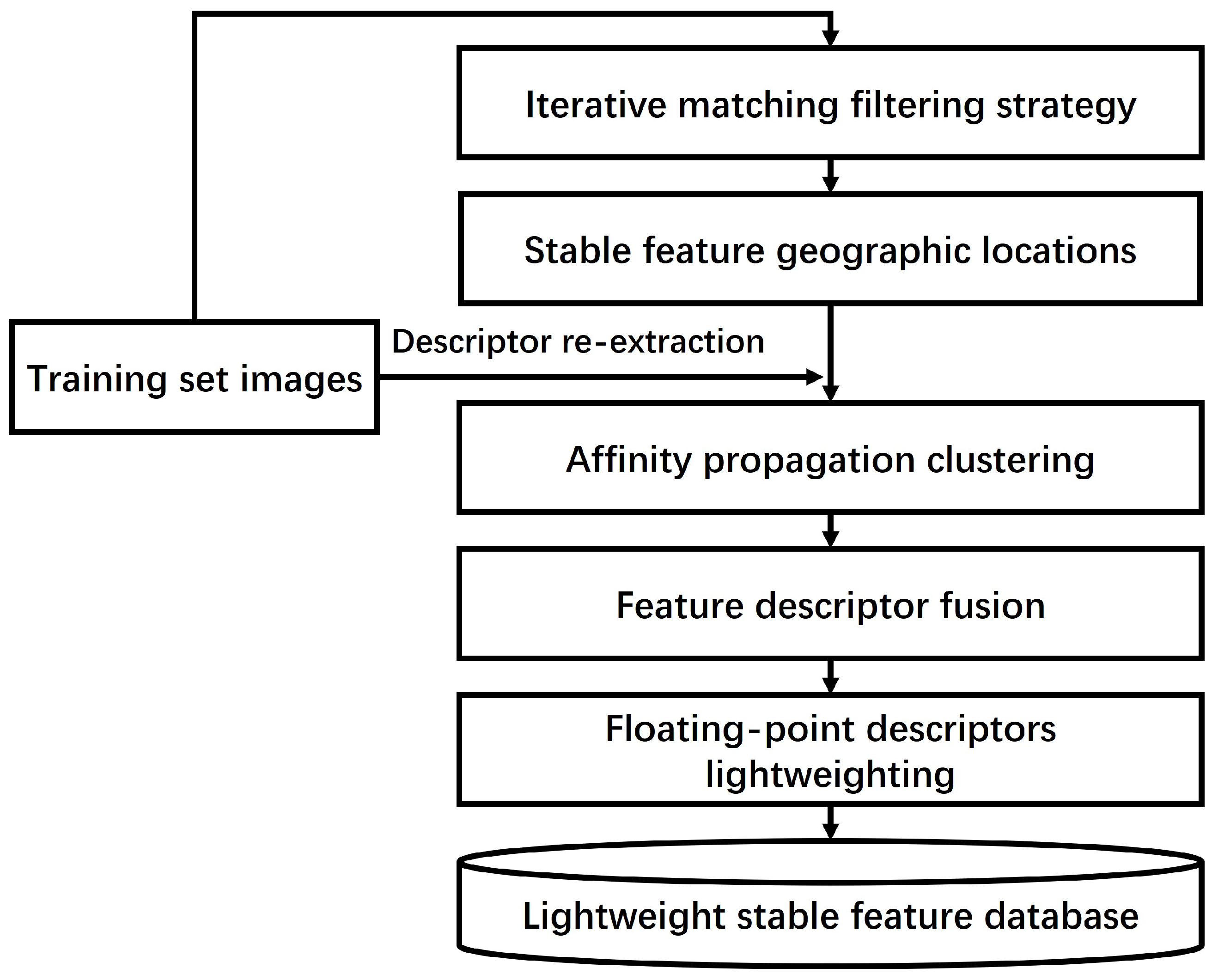
• Stable feature database construction: Building the stable feature database by combining the iterative matching filtering strategy and AP to store non-redundant descriptors under multiple imaging conditions, thus enhancing matching stability.
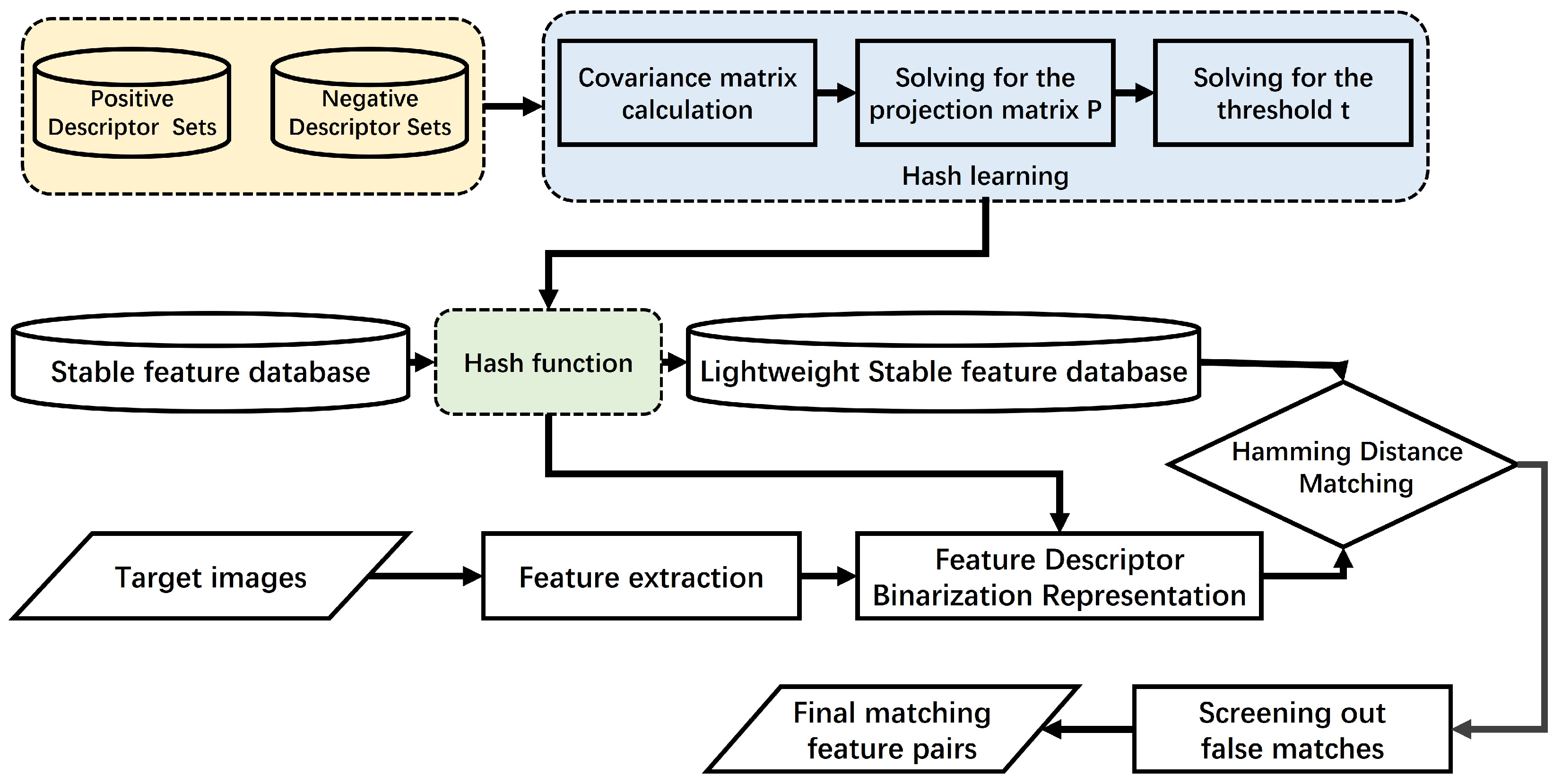
• Lightweight feature descriptor: LDAHash is employed to derive binary descriptors for high-capacity floating-point descriptors, thereby effectively reducing storage demands.
• Feature enrichment in the database: The introduction of multi-scale region features and RIFT to the stable feature databases enriches the type of feature database and extends the applicable scenarios.

The remaining sections of this paper are organized as follows: Section 2.1 describes our proposed improved approach for stable feature database construction based on an iterative matching filtering strategy and AP. Section 2.2 describes the steps for the LDAHash-based floating-point descriptor lightweight. Section 3 and Section 4 conduct the experiments and discuss the results in depth. And finally, Section 5 concludes the paper.

2. Materials and Methods

2.1. Stable Feature Database Construction Based on Iterative Matching Filtering Strategy and Affinity Propagation

This section details the construction of the stable feature database to improve database stability and reduce descriptor redundancy. Initially, the iterative matching filtering strategy is used to determine the accurate geographic locations of stable feature classes [42]. Later, stable feature descriptors are re-extracted from each image in the training set, with each feature point storing descriptors for multiple imaging conditions. Later, we clustered multiple descriptors under each stable feature point using AP and fused descriptors of the same class. This process increases the storage of descriptors for various imaging conditions while reducing redundancy. See Figure 2 for the specific flow chart.

2.1.1. Stable Feature Filtering Based on an Iterative Matching Filtering Strategy

In this subsection, the previously proposed training-feedback mechanism is utilized to iteratively match the feature database, aiming to obtain the locations of relatively stable features and build an initial simple and stable feature database.

Simple and stable feature database construction is undertaken in two steps. Initially, the relevant features are extracted from the geographically accurate reference image, and the pertinent information about these features is stored in the initial feature database. Subsequently, the training images undergo continuous matching with the feature database, leading to updates in the content of the feature database based on matching results, which may involve the addition or deletion of feature points. Throughout the continuous matching iteration process, relatively stable features are identified. The specific information stored in the feature database can be found in

Table 1. Information stored in the simple and stable feature database.

Single Feature Storage Content	Description
Feature Properties	geographic coordinate, response, angle, size, octave
Update Parameters	number of matches (M), number of unmatched matches ($UM$), number of consecutive matches ($CM$), number of consecutive unmatched matches ($CUM$), feature class label
Feature Descriptor	multi-dimensional feature vector

.

First, apply the adaptive histogram equalization preprocessing to the reference image R. Then, extract feature points using the selected feature algorithm. Collect all extracted features to form the feature set $F_0=\{f_1^0,f_2^0,\dots ,f_{n_0}^0\}$ and store them in the initial feature database. Each extracted feature from the reference image is treated as a feature class and labeled accordingly. Here, $f_i^{\mathrm{k}}$ represents the feature class with an index of i in the feature database, and k denotes the number of images input into the feature database. $n_0$ represents the total number of feature classes in the feature set. In the initial feature database, the matching parameters for each feature are set as $M_j=C{M}_j=U{M}_j=CU{M}_j=0$, where $j=0,1,2,\dots ,N_0$. Here, $N_0$ represents the total number of feature points in the feature set $F_0$, and initially, $n_0$ is equal to $N_0$.

Afterward, input the training images $\{S_1,S_2,\dots ,S_N\}$ and match them with the initial feature database, where N represents the number of training images. When inputting the k-th training image $S_k$, retrieve the feature set $F_k=\{f_1^k,f_2^k,\dots ,f_{n_f}^k\}$ from the feature database based on the latitude and longitude of the training image. Then, extract the feature set $T_k=\{t_1^k,t_2^k,\dots ,t_{n_t}^k\}$ from the training image $S_k$ using the same feature extraction method. During the matching process, the successful correspondences between the points are grouped to form the feature classes, and the matching parameters are recorded. If a feature does not find a match, the relevant parameters are also recorded. If a feature matches successfully with a feature class, it is considered a successful match with the corresponding location. The feature set $F_k$ is modified under the condition of valid matches, adjusted based on the matching results with $T_k$ and two predefined thresholds $thre1$ and $thre2$, and then stored in the feature database. Refer to Algorithm 1 for specific algorithmic details, more detailed training steps and parameter settings can be found in reference [42].

We made a simple modification to enhance the likelihood of multiple descriptors within feature classes, and we maintain the $CUM$ of unmatched feature points within successfully matched feature classes unchanged, so it no longer increases compared to the original method [42]. Furthermore, to ensure the accuracy of features within feature classes, during the training-matching process, we ensure that one feature class can only match one feature point in the training image.

The number of feature matches for the same feature class is consistent and can indicate the stability of that feature class to some extent. A higher number of feature matches suggests frequent appearances of the feature class during training iterations, while a lower count indicates fewer successful matches in training. During the training process, feature points with a high number of unmatched matches are eliminated. We continue to utilize the matching number of feature classes as the criterion for filtering stable features. We screen stable feature points with filter match number ($FMN$). For example, $FMN=6$ indicates that only feature classes with a matching frequency greater than or equal to six are extracted. We have previously verified that a higher $FMN$ corresponds to more stable extracted feature classes from the database, yet fewer feature classes are extracted. A limited number of feature classes also cannot achieve a good matching effect. Therefore, we generally set $FMN=6$, which can obtain a certain number of stable feature classes.

Algorithm 1: Feature Database Construction

Figure 3 illustrates the distribution of stabilizing feature points obtained according to the method in this paper using KAZE as an example. Since the degree of overlap between the training images varies, there are relatively few stable feature points in regions with less overlap.

The location of each stable feature class is consistent. Currently, multiple descriptors at the same location are aggregated within the class. However, the descriptors within the set are all similar, representing a typical scenario. To increase the possibility of matching remote sensing images under different imaging conditions, we re-extract the corresponding feature descriptors at the same latitude and longitude positions in each training image after obtaining stable feature positions with high repeatability. In this manner, the descriptors for all imaging conditions within the training set are stored in each stabilization point, which is considered a new feature class.

As depicted in Figure 4, a schematic representation of the neighborhood surrounding several stabilized feature points is presented. The training set composed of multi-source optical images exhibits variations in image performance when trained using the acquired stabilized point locations. It is apparent that despite the similarity in most neighborhood images surrounding the stabilized feature points across different time and viewpoint image sets, they also exhibit diversity, as depicted in Figure 4b,c. If descriptors of stable points are extracted from each training image, we can obtain descriptors not only for individual scenes but also under diverse observational conditions.

Whether the post-training feature class or the re-extracted descriptors for stable point location, multiple similar descriptors are stored in the feature database. In this case, these descriptors need to be processed by clustering and dimensionality reduction. In addition to enabling the extraction of multiple descriptors under various imaging conditions at the same feature location, this approach also facilitates the reduction of storage space and eliminates redundant descriptors.

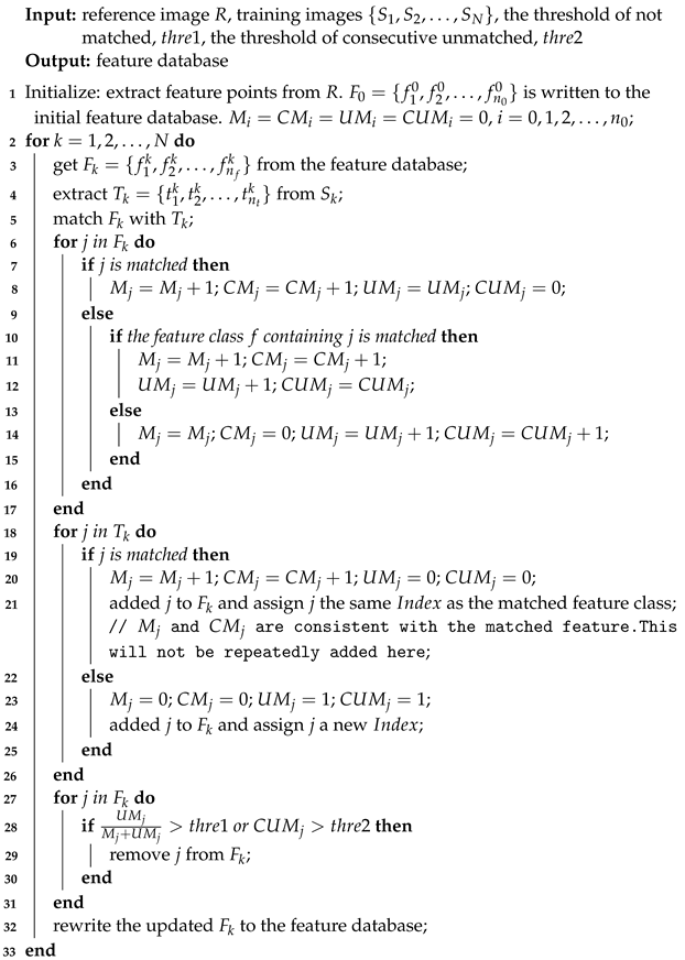
2.1.2. Same-Location Descriptor Clustering and Fusion Based on AP

To eliminate the redundant information in the feature database mentioned above, this subsection details the clustering downscaling of feature descriptors using AP.

AP is well-suited for rapid clustering of high-dimensional, multi-class data. Unlike traditional algorithms, it does not require specifying cluster numbers, broadening its applicability. This explains our choice of utilizing the AP clustering descriptor. Using AP to cluster image feature descriptors within each stable class can differentiate descriptors captured under different imaging conditions, retain a set number of features, and improve matching consistency.

AP considers each data point as a potential clustering center and is primarily based on connecting all descriptors within the same feature class as network nodes. The algorithm computes the clustering centers for different classes of descriptors by employing two types of messages passing within the network: “responsibility” and “availability”. Through iteration, the values of “responsibility” and “availability” for each point are continuously updated until a set number of high-quality clustering centers (denoted as m) are determined. Subsequently, the remaining data points are assigned to their respective clusters.

Set a certain feature class of the input as $x=x_{n\times z}={(x_1,x_2,\dots ,x_n)}^T$. n denotes n descriptors for the same stable feature point location. z is the dimension of the descriptor. First, calculate the similarity matrix of the initial feature descriptors of the same class $S^{\left(0\right)}={\left(s_{ij}\right)}_{n\times n}$ and the initial preference P.

$$s_{ij}=s(i,j)=-d^2(x_i,x_j)=-{∥x_i-x_j∥}^2$$

(1)

$$P=P_{n\times 1}={\left(P_1,P_2,\dots ,P_N\right)}^T$$

(2)

where $s_{ij}$ represents the initial similarity between every pair of feature descriptors within the feature class, while $P_i=P\left(i\right)$ signifies the preference of $x_i$, indicating its reliability as the center of gravity for clustering. The preference is typically set as the median of the similarity values, denoted as $P=median\left(S\right)$.

The iterative update rule for clustering is as follows:

$$r_{t+1}(i,k)=\left\{\begin{array}{c}S(i,k)-{max}_{j\ne k}\{a_t(i,j)+r_t(i,j)\},i\ne k\\ S(i,k)-{max}_{j\ne k}\left\{S(i,j)\right\},i=k\end{array}\right.$$

(3)

$$a_{t+1}(i,k)=\left\{\begin{array}{c}min\{0,r_{t+1}(k,k)+{\sum }_{j\ne i,k}max\left\{r_{t+1}(j,k)\right\},0\},i\ne k\\ {\sum }_{j\ne i,k}max\{r_{t+1}(j,k),0\}\},i=k\end{array}\right.$$

(4)

where the “responsibility” $r(i,k)$ represents the extent to which feature k serves as the exemplar of feature i, taking into account other possible clustering centers for feature i; and the “availability” $a(i,k)$ describes the degree of suitability of feature i to select feature k as its clustering center, taking into account the support of other features for selecting k as a clustering center, with an initial value of zero. t represents the number of iterations.

Meanwhile, the equation above is weakened based on the default damping factor $\lambda =0.5$, primarily utilized to control the convergence rate of the algorithm and ensure the stability of the iterative process.

$$\left\{\begin{array}{c}{r}_{t+1}(i,k)=\lambda ·r_t(i,k)+(1-\lambda )·r_{t+1}(i,k)\\ a_{t+1}(i,k)=\lambda ·a_t(i,k)+(1-\lambda )·a_{t+1}(i,k)\end{array}\right.$$

(5)

The exemplar for feature i is determined by the value of k that maximizes the sum of $a(i,k)$ and $r(i,k)$. Repeatedly execute the aforementioned steps until the clusters and their exemplars achieve stability, or the algorithm terminates when the maximum number of iterations is reached.

Figure 5 shows the clustering of descriptors at four stable feature point locations, taking SURF as a reference. Each stable feature point is chosen to display two neighborhood images that exhibit significant differences after clustering. Each scene encompasses multiple similar descriptors, which have been obtained through AP. Differences in descriptors due to temporal and perspective variations within neighborhood sections of the same feature point location can be observed. Yet, the fluctuations in feature descriptors obtained under similar neighborhood scenes are generally consistent. Hence, utilizing multiple training images in the ground system allows for the clustering of feature descriptors across various temporal phases and viewing angles. This transformation from one-to-one descriptor matching to one-to-many cases enhances the accuracy of feature matching.

Since AP has already performed the classification of descriptors under multiple imaging conditions, descriptors within the same category show significant similarity. As a result, merging similar descriptors is viable, aiding in reducing storage needs and improving computational efficiency. We employ a correlation-weighted average technique to fuse descriptors located at the same stable feature point. Initially, a unique descriptor is selected from each descriptor category. The correlation coefficient between this chosen descriptor and similar descriptors is determined, and the total of these correlation coefficients is calculated. This overall correlation sum is then assigned as the weight (denoted as $w_i)$ for the descriptor. Consequently, descriptors with stronger correlations to feature descriptors within the same class hold higher weights, while those with weaker correlations possess lower weights. The final same-category descriptor fusion results are as follows: In this equation, $\overline{d_i}$ represents the fusion result of similar feature descriptors, and n denotes the total count of these similar descriptors.

$$\overline{d_i}=\frac{{d_i}^1{w}_1+{d_i}^2{w}_2+\cdots \cdots +{d_i}^n{w}_n}{w_1+w_2+\cdots \cdots +w_n}$$

(6)

Figure 6 illustrates a schematic diagram depicting the descriptors of a particular category for multiple feature methods after clustering, along with their fused results represented in histogram form. The figure illustrates the efficacy of fused descriptors in capturing the fluctuations seen in the clustering outcomes of similar descriptors. It is evident from the figure that the similarity level of floating-point descriptors within the same descriptor category is notably greater than that of non-floating-point descriptors. Specific comparisons can be seen between methods such as KAZE and SURF and methods such as AKAZE and ORB. Considering the large change in descriptor fluctuation after the similar fusion of non-floating-point type descriptors, we choose the most relevant one of them as the representative of the class.

2.2. LDAHash-Based Floating-Point Descriptor Lightweighting

This section details the process of lightweighting the descriptors in the feature database using LDAHash to effectively decrease storage space without compromising matching stability. Initially, the unclustered feature database from a training image set is utilized for hash learning. This includes training the projection matrix and threshold vector essential for the hash algorithm. Subsequently, the projection matrix and threshold vector are used to transform the floating-point descriptors in the feature database into binary codes, accomplishing the hash quantization of the floating-point descriptors. Figure 7 depicts the process of lightweighting and matching the feature database using hashing.

2.2.1. LDAHash

This subsection mainly introduces the basic principles of LDAHash.

The hash mapping technique involves converting floating-point descriptors into binary descriptors through the use of affine transformations and sign functions. Firstly, a substantial set of matched feature points is utilized for training to obtain the projection matrix P and threshold vector t for hash learning. Next, the feature vectors are multiplied by the projection matrix P to generate the mapping data. Finally, the mapping data undergoes hashing utilizing the threshold restriction t and a symbolic function, leading to the conversion of the mapping data into binary code.

The relevant formulas are as follows:

$$y=sign(Px+t)$$

(7)

where y represents the $m\times 1$ binary descriptor resulting from mapping, P denotes the $m\times n$ projection matrix, t represents the $m\times 1$ threshold restriction vector, and x represents the floating-point descriptor vector of the feature point.

Implementing hash quantization of descriptors necessitates training on a substantial amount of data to ensure that the hash codes generated from high-dimensional descriptors preserve good similarity properties. The simple feature database trained in Section 2.1.1 can be regarded as a collection of keypoint descriptors, storing both similar and dissimilar features from the training images. All descriptors within the same feature class are treated as belonging to a positive sample class. Simultaneously, descriptors from different feature classes are considered negative samples. Consequently, positive samples constitute the set of homonymous point descriptors T, and negative samples constitute the set of non-homonymous point descriptors F.

The loss function L is defined as follows:

$$L=\alpha E\left\{d_H(y,y^{+})\right|T\}-E\left\{d_H(y,y^{+})\right|F\}$$

(8)

In the equation, $E\{·\}$ represents the expected value, $d_H(·)$ represents the Hamming distance between binary descriptors, $x^{+}$ represents the descriptor of the corresponding feature point in x, and $y^{+}$ represents the binary descriptor of the corresponding feature point in y. $\alpha$ parameter controls trade-offs between false positive and false negative rates. The loss function is optimized to represent the Hamming distance as the square of the second-order moment of the descriptor vector. An alternative expression for the loss function is given below.

$$L=\alpha E\left\{\right||sign(Px+T)-sign(P{x}^{+}+T)|{|}^2\left|T\right\}-E\left\{\right||sign(Px+T)-sign(P{x}^{+}+T)|{|}^2\left|F\right\}$$

(9)

The goal is to minimize the loss function, and it essentially follows the principle of linear discriminant analysis (LDA), which aims to minimize within-class variance and maximize between-class variance.

Due to the non-differentiability of the binary descriptor y when a sign function is applied, direct optimization becomes challenging. Therefore, stepwise optimization can be employed using the projection matrix P and the threshold vector t. The conditions are initially relaxed by eliminating the $sign(·)$ function, allowing for the separate optimization of P. Subsequently, the threshold vector t is determined based on the binary descriptor condition of $y=sign(Px+t)$ utilizing the obtained P matrix.

2.2.2. Projection Matrix P Solution

This subsection describes the method for solving the projection matrix P.

After eliminating the sign function, the loss function can be mathematically represented by the following equation:

$$L=\alpha E\left\{\right||Px-P{x}^{+}|{|}^2\left|T\right\}-E\left\{\right||Px-P{x}^{+}|{|}^2\left|F\right\}$$

(10)

Using property $V^{T}V=tr\left(V{V}^T\right)$ of the vector V, the above equation can be transformed into the following equation:

$$\begin{array}{cc}\hfill L& =\alpha E\{tr\left(\left(P(x-x^{+})\right){\left(P(x-x^{+})\right)}^T\right)|T\}-E\{tr\left(\left(P(x-x^{+})\right){\left(P(x-x^{+})\right)}^T\right)|F\}\hfill \\ \hfill & =\alpha trE\left\{P(x-x^{+}){(x-x^{+})}^T{P}^T\right|T\}-trE\left\{P(x-x^{+}){(x-x^{+})}^T{P}^T\right|F\}\hfill \\ \hfill & =\alpha tr\left\{P{\Sigma }_T{P}^T\right\}-tr\left\{P{\Sigma }_F{P}^T\right\}\hfill \end{array}$$

(11)

where ${\Sigma }_T=E\left\{(x-x^{+}){(x-x^{+})}^T\right|T\}$ represents the covariance matrix that captures the vector difference of the feature descriptors between homonymous points, and ${\Sigma }_F=E\{(x-x^{+})$${(x-x^{+})}^T\left|F\right\}$ represents the covariance matrix that captures the vector difference of the feature descriptors between non-homonymous points.

Subsequently, the multiplication of x by ${\Sigma }_F^{-1/2}$ yields a constant for the second term of the loss function, resulting in the transformation of the loss function into the following equation:

$$L_{min}\propto tr\left\{P{\Sigma }_F^{-1/2}{\Sigma }_T{\Sigma }_F^{-T/2}{P}^T\right\}=tr\left\{P{\Sigma }_R{P}^T\right\}$$

(12)

Here, ${\Sigma }_R$ represents the ratio of the covariance matrices between the descriptors of the positive and negative point sets. It is a symmetric positive semi-definite matrix. The eigen-decomposition of this matrix results in ${\Sigma }_R=US{U}^T$. Where S is a non-negative diagonal matrix, the minimum loss function can be solved by projecting onto the space spanned by the first m smallest eigenvectors of the matrix ${\Sigma }_R$. This procedure ultimately yields the following equation:

$$P{\Sigma }_F^{-1/2}={\left({\Sigma }_R\right)}_m^{-1/2}{\Sigma }_F^{-1/2}={\tilde{S}}_m^{-1/2}{\tilde{U}}^T{\Sigma }_F^{-1/2}$$

(13)

$\tilde{S}$ is a $m\times m$ matrix with the minimum eigenvalue, while $\tilde{U}$ is a $n\times m$ matrix with the corresponding eigenvectors. This completes the calculation of the projection matrix P.

2.2.3. Threshold Vector t Solution

This subsection describes the method for solving the threshold vector t.

After obtaining the projection matrix P, the squared Euclidean distance between vectors $y^{+}$ and y can be computed using an isomorphic method, given the binary descriptor of $y=sign(Px+t)$. Consequently, the loss function can be further redefined as the following equation:

$$\begin{array}{cc}\hfill L& =E\left\{\mathrm{sign}{(Px+t)}^T\mathrm{sign}(P{x}^{+}+t)\right|F\}-\alpha E\left\{\mathrm{sign}{(Px+t)}^T\mathrm{sign}(P{x}^{+}+t)\right|T\}\hfill \\ \hfill & =\sum _{i=1}^m\left\{E\left\{\mathrm{sign}(p_{i}x+t_i)\mathrm{sign}(p_i{x}^{+}+t_i)\right|F\}-\alpha E\left\{\mathrm{sign}(p_{i}x+t_i)\mathrm{sign}(p_i{x}^{+}+t_i)\right|T\}\right\}\hfill \end{array}$$

(14)

Here, $p_i$ represents the i-th row vector of the matrix P, while $p_i$ corresponds to the i-th numerical variable in the threshold vector t.

The minimization of the loss function can essentially be reformulated as the minimization of the following expression:

$$E\left\{\mathrm{sign}(p_{i}x+t_i)\mathrm{sign}(p_i{x}^{+}+t_i)\right|F\}-\alpha E\left\{\mathrm{sign}(p_{i}x+t_i)\mathrm{sign}(p_i{x}^{+}+t_i)\right|T\}$$

(15)

At this stage, the task of solving the threshold vector t can be transformed into a one-dimensional search problem for each independent variable $t_i$. Specifically, it involves determining the false negative rate $FNR\left(t_i\right)$ and the false positive rate $FPR\left(t_i\right)$ of $t_i$, which can be expressed as the following two equations:

$$\begin{array}{cc}\hfill FNR\left(t_i\right)& =Pr(p_{i}x+t_i\le 0 \& \& p_i{x}^{+}+t_i>0|T)\hfill \\ \hfill & +Pr(p_{i}x+t_i>0 \& \& p_i{x}^{+}+t_i\le 0|T)\hfill \end{array}$$

(16)

$$\begin{array}{cc}\hfill FPR\left(t_i\right)& =Pr(p_{i}x+t_i>0 \& \& p_i{x}^{+}+t_i>0|F)\hfill \\ \hfill & +Pr(p_{i}x+t_i\le 0 \& \& p_i{x}^{+}+t_i\le 0|F)\hfill \end{array}$$

(17)

Let $h=-p_{i}x$, $h^{+}=-p_i{x}^{+}$, then we have.

$$\begin{array}{cc}\hfill FNR\left(t_i\right)& =Pr(min\{h,h^{+}\}<t_i\le max\{h,h^{+}\}|T)\hfill \\ \hfill & =1-Pr(t_i\le min\{h,h^{+}\}||max\{h,h^{+}\}<t_i|T)\hfill \\ \hfill & =cdf(min\{h,h^{+}\}|T)-cdf(max\{h,h^{+}\}|T)\hfill \end{array}$$

(18)

$$\begin{array}{cc}\hfill FPR\left(t_i\right)& =Pr(min\{h,h^{+}\}\ge t_i||max\{h,h^{+}\}<t_i|F)\hfill \\ \hfill & =1-Pr(min\{h,h^{+}\}<t_i|F)+Pr(max\{h,h^{+}\}<t_i|F)\hfill \\ \hfill & =1-cdf(min\{h,h^{+}\}|F)+cdf(max\{h,h^{+}\}|F)\hfill \end{array}$$

(19)

In this case, $Pr(·)$ represents the probability function, and $cdf(·)$ denotes the cumulative distribution function. These functions can be approximated by utilizing the minimum-maximum statistical histogram of the projected values h versus $h^{+}$. As a result, the conversion of the loss function leads to the subsequent problem:

$$\underset{t_i}{min}\alpha FNR\left(t_i\right)+FPR\left(t_i\right)$$

(20)

Upon acquiring the projection matrix and threshold vector, we can apply these trained parameters to quantize the descriptors within the feature database. By combining the superior feature description capability of floating-point descriptors with the efficiency advantage of binary descriptors, it becomes possible to save storage space, lower computational costs, efficiently compare descriptor similarity, and achieve high-precision matching. Figure 8 illustrates the process of converting a floating-point descriptor into a binary descriptor.

3. Experiments and Results

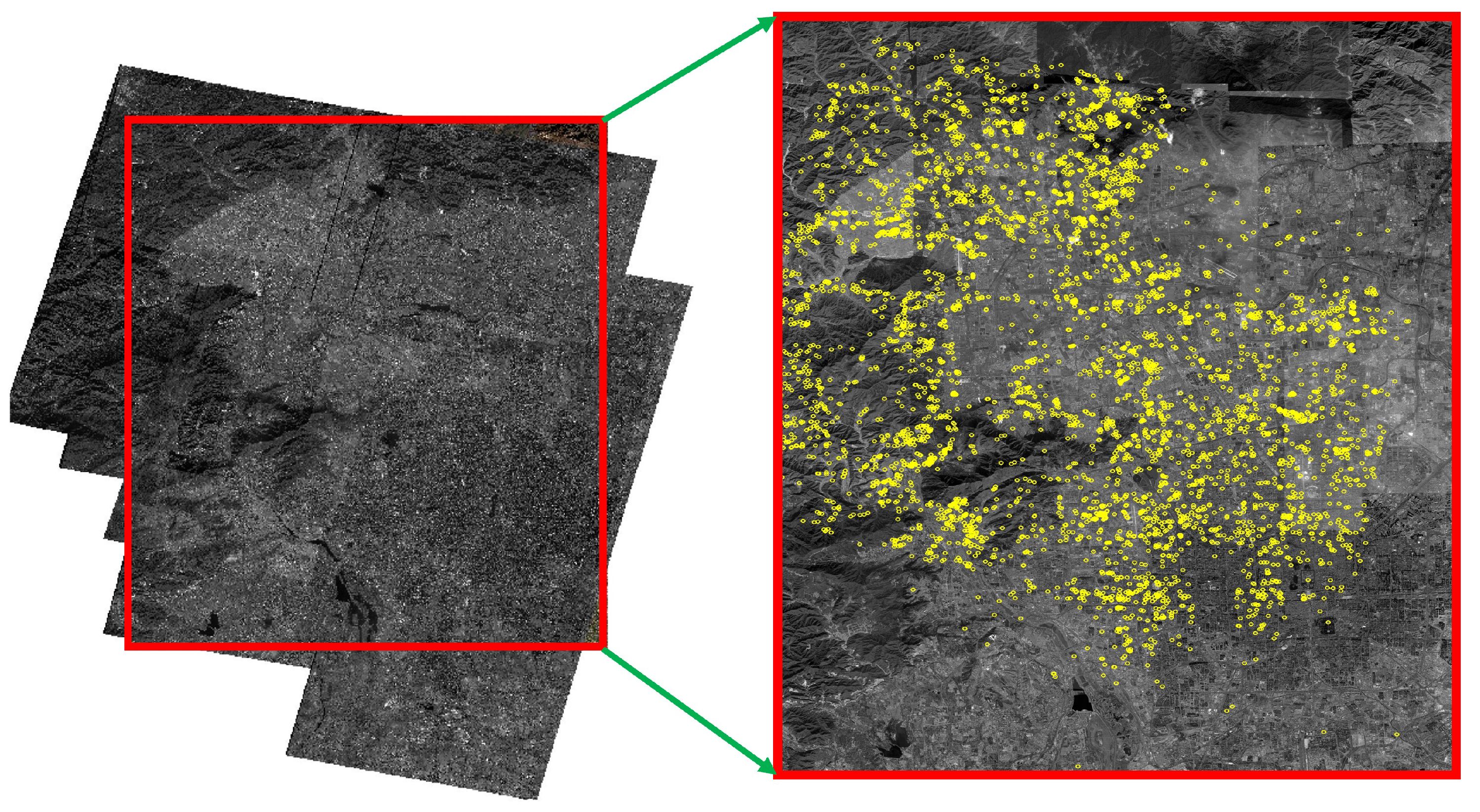
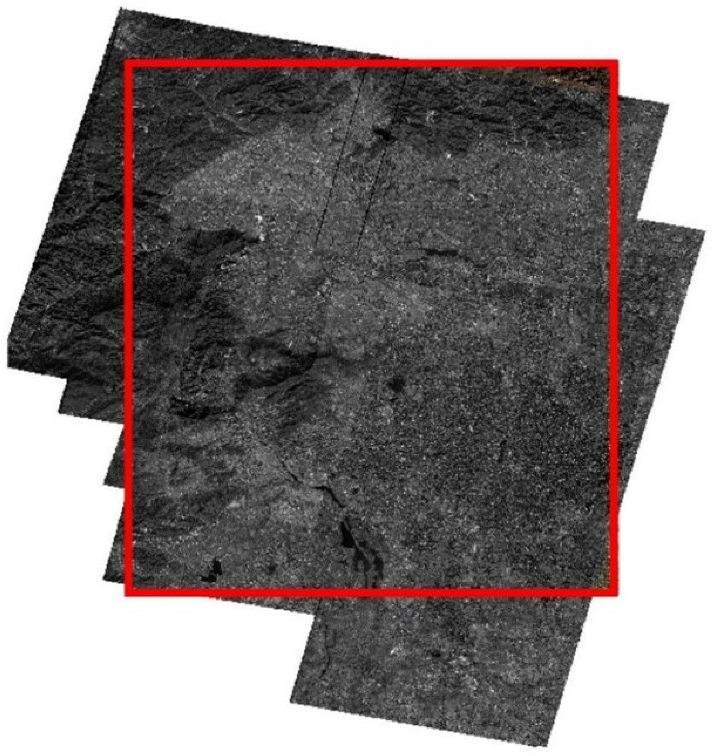
In this section, we will experiment with lightweight stable feature databases constructed using multiple features. These experiments will be conducted on multi-source optical remote sensing images to assess the effectiveness of our proposed method.

3.1. Image Data

In the experiment, a dataset of multi-satellite optical remote sensing images with different perspectives and different time phases, which have a certain overlapping area, is used to verify the proposed method for constructing the feature databases. The experimental area for the dataset is the western region of Beijing, which comprises one reference image, fifty training images, and nine target images. The reference image used in this study is from Google, providing precise geographic locations. Training images include fifty high-resolution Gaofen-2 (GF-2) remote sensing images. Target images are chosen from Jilin-1 (JL-1), Gaofen-1 (GF-1), and GF-2, all being high-resolution remote sensing images, with three images in each category. To ensure effective feature database training and subsequent geometric localization, we pre-align training images, minimizing pixel deviation between the reference image and the training images.

Specific details about the dataset, including its source, number of images, image size, acquisition time, and spatial resolution, are provided in

Table 2. Information for the dataset.

Image	Source	Number	Date	Size (Pixel × Pixel)	Resolution (m)
Reference (A)	Google Earth	1	2016	53,120 × 49,152	1.19
Training (B)	GF-2	50	2016–2022	27,620 × 29,200	0.81
Target (C)	JL-1 (C-1 C-2 C-3)	3	2019–2020	28,651 × 28,720	0.75
	GF-1 (C-4 C-5 C-6)	3	2019–2021	18,236 × 18,190	2
	GF-2 (C-7 C-8 C-9)	3	2019–2021	27,620 × 29,200	0.81

. Figure 9 presents the corresponding diagram, with the red box denoting the coverage area of the reference image.

3.2. Experimental Setup and Evaluation Criterion

In this study, the multi-resolution images are standardized to a consistent resolution using interpolation. The dataset is set to a uniform resolution of 4 m. Considering computer performance and experiment time, setting a 4 m resolution can accelerate the establishment of feature databases and matching of test images while maintaining a certain high resolution. In multi-feature training and matching experiments, a blocking approach with a regional block size of $2500\times 2500$ pixels is used. If matching points in block matching results of a single image are less than 10, it is deemed unstable, and all metrics in the experiment are set to zero.

For point features, we extract 2000 points from each block using the feature algorithm and iteratively match them with the feature database. For region features, we utilize two scales, 4 m and 16 m, to train the extraction of MSER. Selecting 4 m resolution maintains consistency with point feature training. Using identical MSER parameters, opting for a 16 m resolution captures the reference image’s crucial object contours, facilitating comparison with the 4 m resolution for MSER extraction. The minimum area to be extracted is set as 1/10,000 of the area of the region blocks, while the maximum area is limited to 1/100 of the block area. In addition, we control the maximum rate of change to be 0.5.

KAZE and SURF descriptors utilized in the method introduction demonstration are 64-dimensional. For LDAHash experiments, we increase the dimensionality of KAZE and SURF descriptors to 128 to align with SIFT and augment the hash code dimensionality. The FREAK employs the BRISK detection method.

Three quantitative metrics are utilized in this experimental section to assess the performance of the proposed feature database matching method.

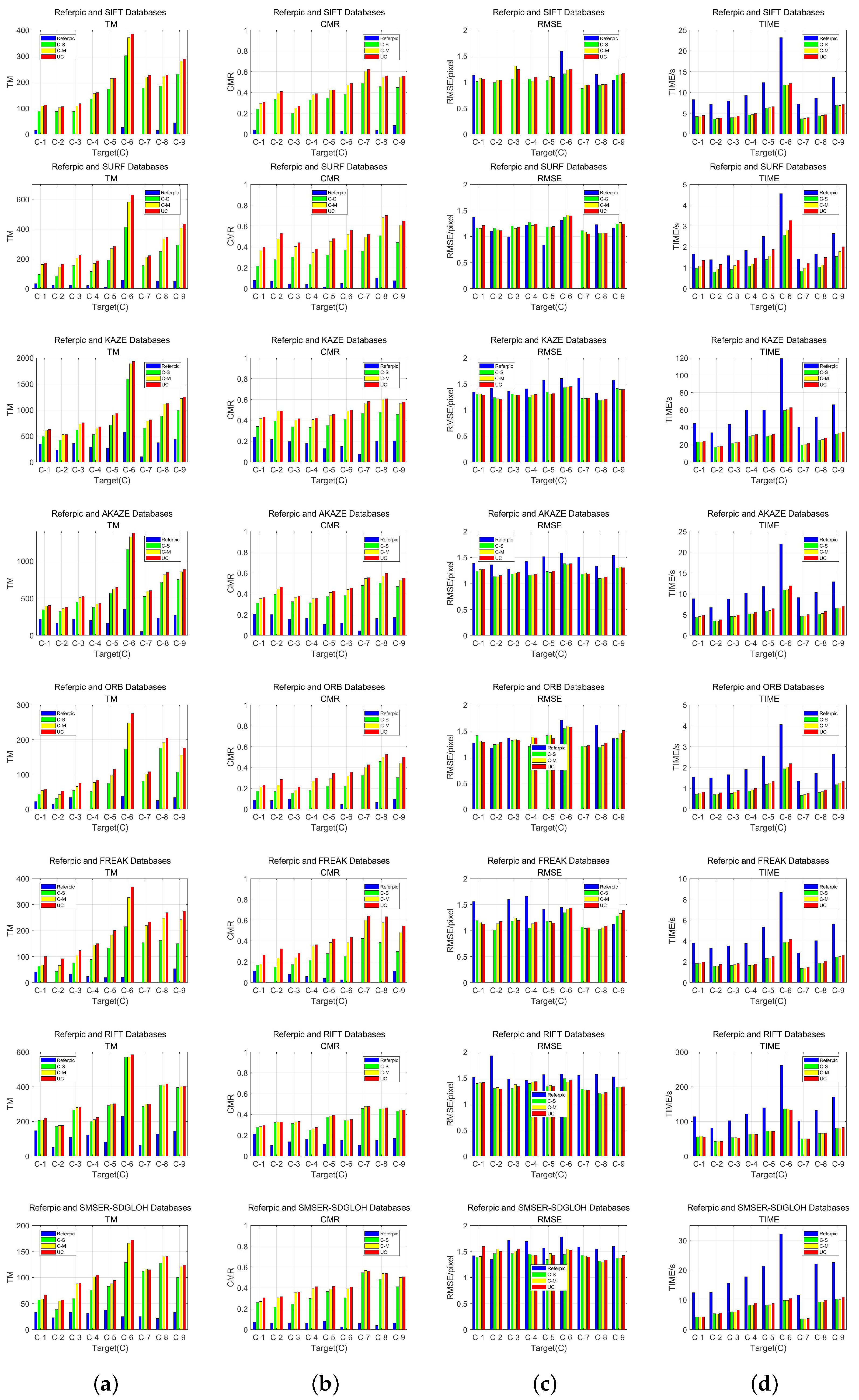
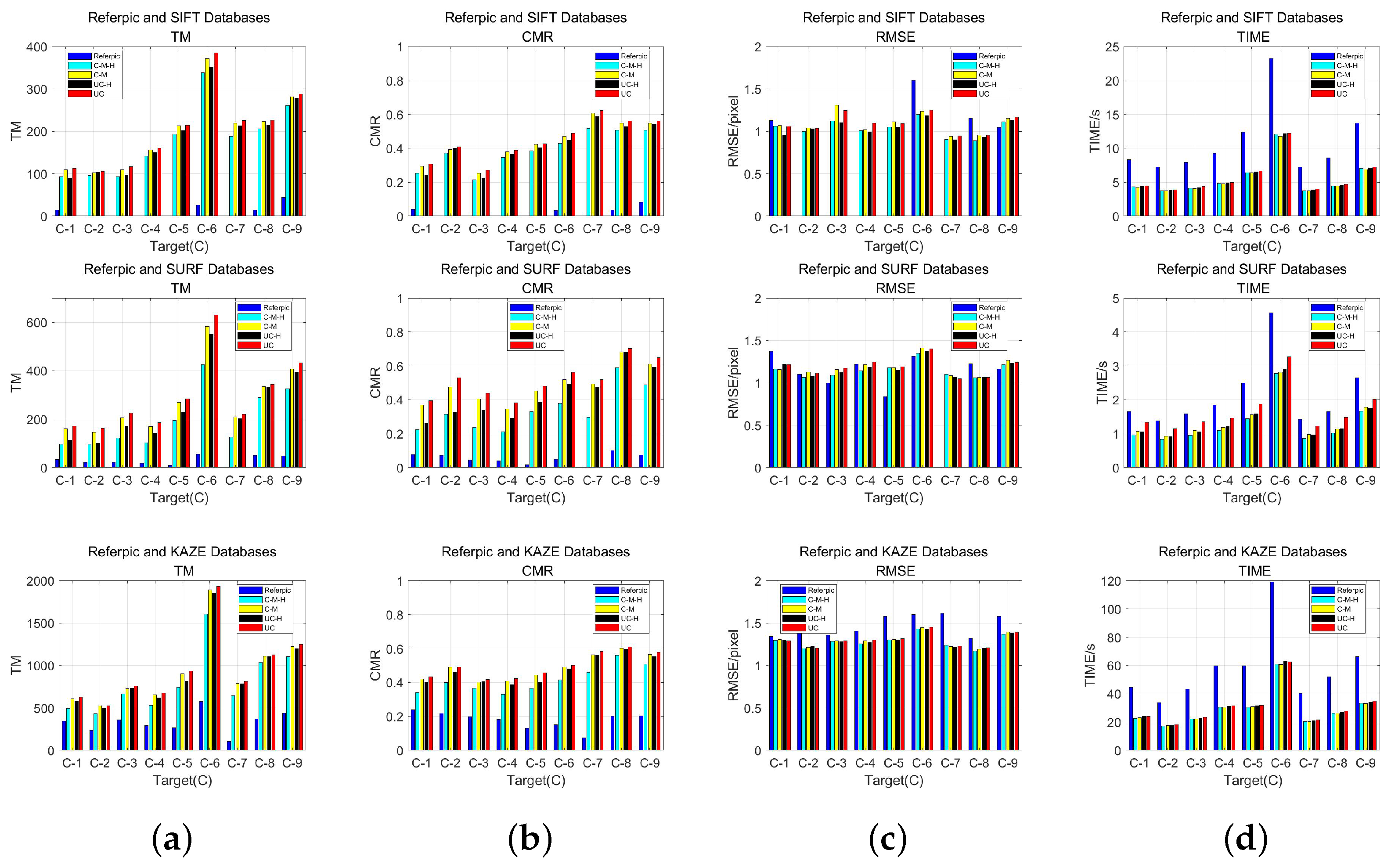
• Correct Matching Ratio (CMR): CMR in this paper is defined as the ratio of the total number of matches (TM) obtained after the false match filtering process to the total number of features ($N_{orig}$) extracted from the feature database. Higher CMR indicates better matching of matching methods. CMR in this paper is calculated at the feature class level. When multiple descriptors in a feature class have matches, they are treated as a single match, considering only the total number of matches for each feature class.

  $$CMR=\frac{TM}{N_{orig}}$$

  (21)
• Root Mean Square Error (RMSE): RMSE is used to reflect the geometric localization accuracy of the feature matching method. Where $(x_i^r,y_i^r)$ denotes the coordinates of the matched features in the reference image or feature database and $(x_i^{t^{\prime }},y_i^{t^{\prime }})$ denotes the corresponding coordinates of the matched points in the target image after geometric correction. The smaller RMSE denotes a higher degree of geometric localization accuracy.

  $$RMSE=\sqrt{\frac{1}{TM}\sum _{i=1}^{TM}\left(\right(x_i^r-x_i^{t^{\prime }}{)}^2+{(y_i^r-y_i^{t^{\prime }})}^2})$$

  (22)
• TIME: TIME is the total time spent on feature extraction and matching between the reference image or feature database and the target image, reflecting the efficiency of the matching method.

3.3. Experiment Analysis

3.3.1. Matching of Stable Feature Databases

This experiment verifies the superiority of the stable feature database proposed in Section 2.1. The experiments used a variety of features to produce multiple feature databases, including SIFT, SURF, KAZE, AKAZE, ORB, FREAK, RIFT, and the stable region features SMSER-SDGLOH [37]. This study involves a comparative analysis of feature database matching and reference image matching. For matching experiments, the number of features extracted from each database was the same as those from the reference image. In this experiment, the quantitative comparison was primarily focused on using the same resolution 4 m.

Compared to matching with the reference image, our stable feature database achieves better matching performance. The matching performance of a few features in a stable database is comparable to that of many features in the reference image. Meanwhile, we compare matching differences in three feature databases: unclustered (UC), clustered multi-descriptor (C-M), and clustered single-descriptor (C-S). Each feature in the C-M feature database stores all fusion results, while each feature in the C-S feature database selects the fusion result of the category with the most descriptors as the representative descriptor. This analysis allows us to further examine the impact of our proposed method.

Hereafter, we will present our findings and undertake both qualitative and quantitative analyses.

Figure 10 illustrates stable features obtained using multi-feature approaches. These stable features are obtained after undergoing training with an iterative filtering strategy. The figure shows that KAZE and AKAZE generate more stable feature points for point features under the same training conditions, consistent with our previous study. However, in terms of region features, the limited number of stable regions remains after iterative matching through the feature database. There could be several reasons for this. First, the limitation on the number of homogeneous region features can only be realized by thresholding, making it difficult to accurately control the number. In addition, the number of regions in an image is inherently small compared to point features, and the initial extracted MSERs in the training images are relatively sparse.

Table 3. Comparison of storage space (MB) before and after clustering of multiple feature databases.

Database Type	SIFT	SURF	KAZE	AKAZE	ORB	FREAK	RIFT	SMSER-SDGLOH-4 m
Unclustered (UC)	16.90	26.90	92.00	14.50	2.58	5.29	63.00	12.90
Clustered Multi-descriptor (C-M)	8.42	12.70	46.80	5.29	0.86	1.46	33.60	5.99
Clustered Single-descriptor (C-S)	2.18	3.32	11.50	0.99	0.19	0.31	7.76	1.63

shows the comparison of the storage space of different feature databases. After clustering fusion, the storage space of the stable feature database is significantly reduced compared to before clustering. Furthermore, storing a single descriptor at a specific point location requires significantly less space than storing multiple descriptors.

We individually match the feature databases with the target image set and compare the results with the reference image matching to validate the effectiveness of our proposed method. The experimental results will be illustrated in Figure 11. Through the analysis of Figure 11, the following findings were observed.

Comparing stable feature database with reference image. The TM and CMR of the stable feature database matching significantly surpass those of direct matching with the reference image for the same number of extracted features. In most cases, the stable feature database shows lower RMSE compared to matching with the reference image, indicating higher registration accuracy. Furthermore, in contrast to potential instability in reference image matching, our feature database matching ensures successful matching of each target image without compromising accuracy. For example, matching the C-7 image with the reference image using a specified number of features (e.g., SIFT, SURF, ORB) did not produce stable results. However, successes were achieved by matching with the stable feature database generated by the corresponding method. Additionally, the matching efficiency is increased by the feature databases, which saves time by avoiding the need to run the feature extraction again to extract features from the reference image.

Comparing the C-M feature database with the C-S feature database. Observing the storage of multiple descriptors at stable feature point locations reveals higher TM and CMR compared to storing a single descriptor. Storing multiple descriptors for imaging conditions at the same feature point location can enhance matching possibilities by transitioning from the traditional one-to-one matching of descriptors to one-to-many matching. This is one of the advantages of feature database matching over single reference image matching. The RMSE of the C-M feature database matching and the C-S feature database matching are not significantly different. In terms of TIME, because the C-S feature database stores less content than the C-M feature database, the matching time is shorter, but it is not very apparent in the graph.

Comparing the C-M feature database with the UC feature database. Before clustering, each feature in the feature database stores redundant multiple imaging condition descriptors. Although the UC feature database matching effect is slightly better than that of the C-M feature database, there is much redundant information. The C-M feature database retains feature descriptors under different imaging conditions while significantly reducing storage space in the feature database. The C-M feature database yields results that are highly similar to those of the UC feature database. Taking into account the storage space and the matching results, the C-M feature database is more comprehensive.

From the figure of experimental comparison, we can also have some interesting findings. For the RIFT database, the impact on matching effectiveness is minimal before and after clustering, regardless of the quantity of stored descriptors. Particularly noteworthy is the comparison of matching effectiveness between the C-S feature database and the C-M feature database based on RIFT. In this context, the matching accuracy and the number of correct matches for RIFT remain largely unaffected. This observation indirectly highlights the advantages of RIFT. However, in terms of time efficiency, RIFT does not show significant superiority over other features, especially when considering the need to achieve real-time performance. Similarly, blob features such as KAZE, AKAZE, SIFT, and SURF exhibit relatively minor changes in matching effectiveness before and after clustering, compared to corner features such as ORB and FREAK. This observation underscores the stability advantages of these features in conjunction with corner points and binary descriptors. However, the obvious combination of corner points and binary codes has stronger timeliness, which gives it an advantage in real-time matching. In the future, we will further explore techniques such as parallel CUDA acceleration or on-board hardware acceleration to improve the computational efficiency of feature databases.

3.3.2. Matching of Lightweight and Stable Feature Databases

This experiment verifies the superiority of the lightweight and stable feature database proposed in Section 2.2. Classical blob feature algorithms, such as SIFT, SURF, and KAZE, which are known for their floating-point descriptors, were selected for hash quantization experiments to ensure stable feature point acquisition and lightweight feature representations.

Our experiment aims to convert floating-point descriptors of the same dimension into binary hash codes (0, 1) of equivalent dimension. For instance, the 128-dimensional floating-point descriptor of SIFT occupies $128\times 4$, i.e., 512 bytes, when stored in a computer. However, post conversion to hash code, the resulting vector is 128 bits, equal to 16 bytes. This represents a storage space reduction of 97% compared to the original. The conversion from Euclidean distance matching to Hamming distance matching can also improve the matching efficiency to some extent.

Table 4. Comparison of storage space (MB) before and after LDAHash.

Database Type	SIFT	SURF	KAZE
Unclustered (UC)	16.90	26.90	92.00
Unclustered-Hash (UC-H)	1.83	2.43	9.37
Clustered Multi-descriptor (C-M)	8.42	12.70	46.80
Clustered Multi-descriptor-Hash (C-M-H)	0.60	0.83	3.50

shows a schematic comparison of the storage space of the stable feature database before and after LDAHash. From the table, it can be seen that the storage space of classical feature floating-point descriptors is significantly reduced after clustering, especially after LDAHash.

Figure 12 shows the result diagrams of our lightweight stable feature databases matching experiments using the three methods of SURF, SIFT, and KAZE. By analyzing the experimental results, we observe that the TM and CMR of the feature databases show a decreasing trend after the LDAHash quantization process. The observed trend may be attributed to information loss caused by LDAHash. The purpose of hash quantization is to convert a high-dimensional descriptor into a low-dimensional binary hash code for more efficient similarity comparisons. However, this mapping invariably results in the loss of certain details from the original descriptors, and multiple distinct descriptors can be assigned the same binary code. Consequently, this situation can lead to a decline in the accuracy of matches in certain scenarios.

Although there is a declining trend, it is important to note that the quantization-based matching method still performs significantly better than a direct matching method that relies on a reference image alone. Furthermore, there is no substantial impact on the accuracy of registration while achieving a significant reduction in storage space. This result further demonstrates the potential of LDAHash as an effective means of feature processing that maintains relatively high matching accuracy while reducing feature database storage requirements.

We can also observe that the lightweight feature database takes significantly less time to match, and this trend is more significant, especially in SURF. SURF exhibits a short computation time for feature extraction, and the time saved by the hash-processed algorithm constitutes a significant portion of this time. Consequently, LDAHash shows a distinct time advantage in SURF matching. In contrast, KAZE has longer extraction times and generates numerous stable feature points, resulting in a relatively minor reduction in matching time through hashing.

The obtained experimental results provide useful insights for further optimization of future matching strategies and lightweight methods. Under specific application needs and performance requirements, it is acceptable to sacrifice a small percentage of matching correctness for higher storage efficiency or faster matching speed within a certain range. Therefore, when choosing the lightweight stable feature database to be used, the matching accuracy and computational efficiency need to be carefully weighed to meet the different needs in practical applications. In the future, we will prioritize targeting specific application scenarios by adjusting the parameters of the hash function or implementing additional optimization strategies. This will improve the differentiation and matching performance of the hash code.

4. Discussion

In this discussion section, our primary focus is to compare the distinctions between region feature databases and point feature databases, and to outline prospects for future enhancements of feature databases.

We enriched the experimental feature database by incorporating multi-scale region feature databases. The setting of the region feature database is similar to that of the point feature database. In the region feature database, we will also store the parameters such as the height, width, and angle of the ellipse obtained from the fitting of the stabilized SMSERs. This not only comprehensively describes region features but also enhances the expressive power of the region feature database.

Point features and region features have distinct characteristics and advantages. As shown in Figure 13, the stable point features and region features obtained from training exhibit a complementary relationship. Region features primarily capture homogeneous ground features, providing richer contextual information and exhibiting less susceptibility to change as they match a set of related pixel points as a whole. The stabilized regions obtained through training are sparse and have relatively low registration accuracy, suitable for initial point localization on a large scale. While point features focus on capturing rich texture information in the image, they are discrete points that can be densely extracted from an image. Thus, they are suitable for tasks requiring precise and dense localization, such as change detection, where high registration accuracy is essential. However, they are susceptible to noise interference.

Table 5. Point Features vs. Region Features.

Feature Attributes	Regions	Points
Feature Composition	a set of interconnected pixel points	discrete points
Distribution Density	sparse	dense
Registration Accuracy	relatively lower	higher
Stability	small variation	susceptible to noise
Application	rough localization of a wide range of primary points	fine and dense localization

shows the comparison between the region features and the point features obtained from our experimental analysis of the feature database.

It should be noted that training at different scales yields distinct and stable region features, as shown in Figure 13b,c, with resolutions of 4 m and 16 m, respectively. We obtained different stable region distributions by training at different scales with the same MSER parameters. This means that we can choose the appropriate feature database according to the scale and characteristics of the images to be matched to optimize the matching results. This aspect will become an important direction for future research, and we will deeply explore the differences in the stabilized region features obtained by training at different resolutions and scales, and provide a more flexible and precise feature selection strategy for practical applications.

This paper mainly uses multiple feature methods to validate the universality of feature databases, but does not conduct experiments by incorporating multiple features into the same feature database. Later, matching can also be enhanced by storing multiple point features or region features in the same area. In complex scenes, point features may be more suitable if the image structure is primarily composed of small yet significant feature points. Conversely, for images lacking distinct feature points but containing prominent homogeneous regions, region features may offer stronger registration capabilities. By exploring the advantages and limitations of point features and region features, we can gain a deeper understanding of their applicability in different scenarios and tasks, providing useful guidance for future feature database construction and selection of image matching. Furthermore, it is beneficial to enhance the diversity of feature information in the feature database. For instance, alongside storing texture information of the region feature, storing contour information can be valuable in enhancing the probability of matching the region feature [45].

The outcome of feature database matching is also closely linked to the training set. The selection of different training sets significantly impacts the stable feature points and descriptors obtained. The properties of descriptors in the feature database are directly influenced by multiple factors of the training dataset, including the selection of geographic features, time span, image types, and image quality, etc. [46,47]. This flexibility allows us to comprehensively consider the performance of different feature types and different training sets in experiments. We will explore these issues in more depth in future research.

5. Conclusions

In this study, we develop lightweight and stable feature databases. Our approach combines AP and LDAHash techniques to enhance the simplicity and stability of the feature databases. This enables us to obtain lightweight and stable descriptors that can efficiently handle multi-imaging conditions while adapting to diverse time-phase and viewing perspectives with reduced redundancy. In addition to the original point-based feature method, we introduce multi-scale region features to enhance the overall generalizability of the features in the database. Our method offers the following key advantages:

• Feature stability: The stability of the features stored in the database is somewhat improved through the implementation of the training set filtering strategy.
• Descriptions richness: Utilizing AP to obtain multiple imaging condition descriptors at the same point to enhance matching possibilities.
• Storage efficiency: AP reduces redundancy in the feature databases, while LDAHash converts floating-point descriptors into binary representations, resulting in significant space savings.
• Universality of multiple features: Our feature databases can incorporate various features, including point features and region features. This flexibility allows for a more comprehensive reference in practical applications.

References

1. Du, Q.; Nekovei, R. Fast real-time onboard processing of hyperspectral imagery for detection and classification. J. Real-Time Image Process. 2009, 4, 273–286. [Google Scholar] [CrossRef]
2. Long, T.; Jiao, W.; He, G.; Yin, R.; Wang, G.; Zhang, Z. Block Adjustment With Relaxed Constraints From Reference Images of Coarse Resolution. IEEE Trans. Geosci. Remote Sens. 2020, 58, 7815–7828. [Google Scholar] [CrossRef]
3. Lai, G.; Zhang, Y.; Tong, X.; Wu, Y. Method for the Automatic Generation and Application of Landmark Control Point Library. IEEE Access 2020, 8, 112203–112219. [Google Scholar] [CrossRef]
4. Pi, Y.; Xie, B.; Yang, B.; Zhang, Y.; Li, X.; Wang, M. On-orbit geometric calibration of Linear push-broom optical satellite based on sparse GCPs. J. Geod. Geoinf. Sci. 2020, 3, 64. [Google Scholar]
5. Wang, T.; Zhang, G.; Li, D.; Tang, X.; Jiang, Y.; Pan, H.; Zhu, X. Planar block adjustment and orthorectification of ZY-3 satellite images. Photogramm. Eng. Remote Sens. 2014, 80, 559–570. [Google Scholar] [CrossRef]
6. Liu, D.; Zhou, G.; Zhang, D.; Zhou, X.; Li, C. Ground control point automatic extraction for spaceborne georeferencing based on FPGA. IEEE J. Sel. Top. Appl. Earth Obs. Remote Sens. 2020, 13, 3350–3366. [Google Scholar] [CrossRef]
7. Wang, M.; Zhang, Z.; Zhu, Y.; Dong, Z.; Li, Y. Embedded GPU implementation of sensor correction for on-board real-time stream computing of high-resolution optical satellite imagery. J. Real-Time Image Process. 2018, 15, 565–581. [Google Scholar] [CrossRef]
8. Salazar, C.; Gonzalez-Llorente, J.; Cardenas, L.; Mendez, J.; Rincon, S.; Rodriguez-Ferreira, J.; Acero, I.F. Cloud Detection Autonomous System Based on Machine Learning and COTS Components On-Board Small Satellites. Remote Sens. 2022, 14, 5597. [Google Scholar] [CrossRef]
9. Yang, J.; Zhao, Z. A fast geometric rectification of remote sensing imagery based on feature ground control point database. WSEAS Trans. Comput. 2009, 8, 195–204. [Google Scholar]
10. Bay, H.; Tuytelaars, T.; Van Gool, L. Surf: Speeded up robust features. In Proceedings of the Computer Vision–ECCV 2006: 9th European Conference on Computer Vision, Graz, Austria, 7–13 May 2006; Proceedings, Part I 9. Springer: Berlin/Heidelberg, Germany, 2006; pp. 404–417. [Google Scholar]
11. Ji, S.; Zhang, Y.; Dong, Y.; Fan, D. Spaceborne lightweight image control points generation method. Acta Geod. Et Cartogr. Sin. 2022, 51, 413–425. [Google Scholar]
12. Lowe, D.G. Distinctive image features from scale-invariant keypoints. Int. J. Comput. Vis. 2004, 60, 91–110. [Google Scholar] [CrossRef]
13. Kelman, A.; Sofka, M.; Stewart, C.V. Keypoint descriptors for matching across multiple image modalities and non-linear intensity variations. In Proceedings of the 2007 IEEE Conference on Computer Vision and Pattern recognition, Minneapolis, MN, USA, 17–22 June 2007; pp. 1–7. [Google Scholar]
14. Schowengerdt, R.A. CHAPTER 8—Image Registration and Fusion. In Remote Sensing (Third Edition); Schowengerdt, R.A., Ed.; Academic Press: Burlington, VT, USA, 2007; pp. 355–385, XXIV–XXVI. [Google Scholar] [CrossRef]
15. Feng, R.; Du, Q.; Li, X.; Shen, H. Robust registration for remote sensing images by combining and localizing feature-and area-based methods. ISPRS J. Photogramm. Remote Sens. 2019, 151, 15–26. [Google Scholar] [CrossRef]
16. Sedaghat, A.; Mokhtarzade, M.; Ebadi, H. Uniform robust scale-invariant feature matching for optical remote sensing images. IEEE Trans. Geosci. Remote Sens. 2011, 49, 4516–4527. [Google Scholar] [CrossRef]
17. Alcantarilla, P.F.; Bartoli, A.; Davison, A.J. KAZE features. In Proceedings of the Computer Vision–ECCV 2012: 12th European Conference on Computer Vision, Florence, Italy, 7–13 October 2012; Proceedings, Part VI 12. Springer: Berlin/Heidelberg, Germany, 2012; pp. 214–227. [Google Scholar]
18. Alcantarilla, P.F.; Solutions, T. Fast explicit diffusion for accelerated features in nonlinear scale spaces. IEEE Trans. Patt. Anal. Mach. Intell 2011, 34, 1281–1298. [Google Scholar]
19. Mikolajczyk, K.; Schmid, C. A performance evaluation of local descriptors. IEEE Trans. Pattern Anal. Mach. Intell. 2005, 27, 1615–1630. [Google Scholar] [CrossRef] [PubMed]
20. Tola, E.; Lepetit, V.; Fua, P. Daisy: An efficient dense descriptor applied to wide-baseline stereo. IEEE Trans. Pattern Anal. Mach. Intell. 2009, 32, 815–830. [Google Scholar]
21. Sedaghat, A.; Ebadi, H. Remote sensing image matching based on adaptive binning SIFT descriptor. IEEE Trans. Geosci. Remote Sens. 2015, 53, 5283–5293. [Google Scholar] [CrossRef]
22. Rublee, E.; Rabaud, V.; Konolige, K.; Bradski, G. ORB: An efficient alternative to SIFT or SURF. In Proceedings of the 2011 International Conference on Computer Vision, Barcelona, Spain, 6–13 November 2011; pp. 2564–2571. [Google Scholar]
23. Leutenegger, S.; Chli, M.; Siegwart, R.Y. BRISK: Binary robust invariant scalable keypoints. In Proceedings of the 2011 International Conference on Computer Vision, Barcelona, Spain, 6–13 November 2011; pp. 2548–2555. [Google Scholar]
24. Alahi, A.; Ortiz, R.; Vandergheynst, P. Freak: Fast retina keypoint. In Proceedings of the 2012 IEEE Conference on Computer Vision and Pattern Recognition, Providence, RI, USA, 16–21 June 2012; pp. 510–517. [Google Scholar]
25. Feng, R.; Shen, H.; Bai, J.; Li, X. Advances and opportunities in remote sensing image geometric registration: A systematic review of state-of-the-art approaches and future research directions. IEEE Geosci. Remote Sens. Mag. 2021, 9, 120–142. [Google Scholar] [CrossRef]
26. Ye, Y.; Shan, J.; Bruzzone, L.; Shen, L. Robust registration of multimodal remote sensing images based on structural similarity. IEEE Trans. Geosci. Remote Sens. 2017, 55, 2941–2958. [Google Scholar] [CrossRef]
27. Fan, J.; Wu, Y.; Li, M.; Liang, W.; Cao, Y. SAR and optical image registration using nonlinear diffusion and phase congruency structural descriptor. IEEE Trans. Geosci. Remote Sens. 2018, 56, 5368–5379. [Google Scholar] [CrossRef]
28. Li, J.; Hu, Q.; Ai, M. RIFT: Multi-modal image matching based on radiation-variation insensitive feature transform. IEEE Trans. Image Process. 2019, 29, 3296–3310. [Google Scholar] [CrossRef] [PubMed]
29. Viswanathan, D.G. Features from accelerated segment test (fast). In Proceedings of the 10th Workshop on Image Analysis for Multimedia Interactive Services, London, UK, 6–8 May 2009; pp. 6–8. [Google Scholar]
30. Harris, C.; Stephens, M. A combined corner and edge detector. In Proceedings of the Alvey Vision Conference, Manchester, UK, September 1988; Citeseer: Princeton, NJ, USA, 1988; Volume 15, pp. 147–152. [Google Scholar]
31. Tuytelaars, T.; Mikolajczyk, K. Local invariant feature detectors: A survey. Found. Trends® Comput. Graph. Vis. 2008, 3, 177–280. [Google Scholar] [CrossRef]
32. Tuytelaars, T.; Van Gool, L.; Mirmehdi, M.; Thomas, B.T. Wide baseline stereo matching based on local, affinely invariant regions. In Proceedings of the BMVC, Bristol, UK, 11–14 September 2000; British Machine Vision Association: Durham, UK, 2000. [Google Scholar]
33. Tuytelaars, T.; Van Gool, L. Matching widely separated views based on affine invariant regions. Int. J. Comput. Vis. 2004, 59, 61–85. [Google Scholar] [CrossRef]
34. Matas, J.; Chum, O.; Urban, M.; Pajdla, T. Robust wide-baseline stereo from maximally stable extremal regions. Image Vis. Comput. 2004, 22, 761–767. [Google Scholar] [CrossRef]
35. Liu, L.; Tuo, H.; Xu, T.; Jing, Z. Multi-spectral image registration and evaluation based on edge-enhanced MSER. Imaging Sci. J. 2014, 62, 228–235. [Google Scholar] [CrossRef]
36. Martins, P.; Carvalho, P.; Gatta, C. On the completeness of feature-driven maximally stable extremal regions. Pattern Recognit. Lett. 2016, 74, 9–16. [Google Scholar] [CrossRef]
37. Zhao, Z.; Wang, F.; You, H. Robust Region Feature Extraction with Salient MSER and Segment Distance-weighted GLOH for Remote Sensing Image Registration. IEEE J. Sel. Top. Appl. Earth Obs. Remote Sens. 2023, 17, 2475–2488. [Google Scholar] [CrossRef]
38. Ordóñez, Á.; Acción, Á.; Argüello, F.; Heras, D.B. HSI-MSER: Hyperspectral Image Registration Algorithm Based on MSER and SIFT. IEEE J. Sel. Top. Appl. Earth Obs. Remote Sens. 2021, 14, 12061–12072. [Google Scholar] [CrossRef]
39. Śluzek, A. Improving performances of MSER features in matching and retrieval tasks. In Proceedings of the Computer Vision–ECCV 2016 Workshops, Amsterdam, The Netherlands, 8–10 and 15–16 October 2016; Proceedings, Part III 14. Springer: Berlin/Heidelberg, Germany, 2016. [Google Scholar]
40. Zhang, Q.; Wang, Y.; Wang, L. Registration of images with affine geometric distortion based on maximally stable extremal regions and phase congruency. Image Vis. Comput. 2015, 36, 23–39. [Google Scholar] [CrossRef]
41. Zhang, Y.; Guo, Y.; Gu, Y. Robust feature matching and selection methods for multisensor image registration. In Proceedings of the 2009 IEEE International Geoscience and Remote Sensing Symposium, Cape Town, South Africa, 12–17 July 2009; Volume 3, p. III-255. [Google Scholar]
42. Zhao, Z.; Long, H.; You, H. An Optical Remote Sensing Image Matching Method Based on the Simple and Stable Feature Database. Appl. Sci. 2023, 13, 4632. [Google Scholar] [CrossRef]
43. Frey, B.J.; Dueck, D. Clustering by passing messages between data points. Science 2007, 315, 972–976. [Google Scholar] [CrossRef] [PubMed]
44. Strecha, C.; Bronstein, A.; Bronstein, M.; Fua, P. LDAHash: Improved matching with smaller descriptors. IEEE Trans. Pattern Anal. Mach. Intell. 2011, 34, 66–78. [Google Scholar] [CrossRef] [PubMed]
45. Cheng, L.; Pian, Y.; Chen, Z.; Jiang, P.; Liu, Y.; Chen, G.; Du, P.; Li, M. Hierarchical filtering strategy for registration of remote sensing images of coral reefs. IEEE J. Sel. Top. Appl. Earth Obs. Remote Sens. 2016, 9, 3304–3313. [Google Scholar] [CrossRef]
46. Jiang, X.; Ma, J.; Fan, A.; Xu, H.; Lin, G.; Lu, T.; Tian, X. Robust feature matching for remote sensing image registration via linear adaptive filtering. IEEE Trans. Geosci. Remote Sens. 2020, 59, 1577–1591. [Google Scholar]
47. Ghiasi, Y.; Duguay, C.R.; Murfitt, J.; Asgarimehr, M.; Wu, Y. Potential of GNSS-R for the Monitoring of Lake Ice Phenology. IEEE J. Sel. Top. Appl. Earth Obs. Remote Sens. 2023, 17, 660–673. [Google Scholar] [CrossRef]
Figure 1. Flowchart of the methodology in this paper.
Remotesensing 16 01237 g001
Figure 2. Stable feature database construction flow based on iterative matching filtering strategy and AP.
Remotesensing 16 01237 g002
Figure 3. Stable KAZE points viewable obtained by the iterative matching filtering strategy. The yellow dots represent the relatively stable KAZE feature points that remain after iterative matching and filtering.
Remotesensing 16 01237 g003
Figure 4. Schematic of the neighborhood of stable feature sites at the same location under different imaging conditions (we discharged the scenes with similar individual feature sites together). Six stable feature points, labeled as (af), are selected, and ten image neighborhoods are chosen for each feature point to facilitate comparison.
Remotesensing 16 01237 g004
Figure 5. The SURF descriptors are employed as an illustrative example to analyze the variability among descriptors in the clustering results. Four sets of scenarios were selected to demonstrate cases at the same geographical location under different imaging conditions, labeled as (ad). Each image set displays two distinct geospatial representations at the same feature location, along with corresponding fluctuations in descriptors post-clustering.
Remotesensing 16 01237 g005
Figure 6. Diagram of multi-feature fusion. Each feature algorithm includes three images: left shows post-clustered descriptors of a category, middle displays the fused descriptor, and right provides a comparison. (a) SIFT. (b) SURF. (c) KAZE. (d) AKAZE. (e) ORB. (f) FREAK.
Remotesensing 16 01237 g006
Figure 7. The process of lightweighting and matching the feature database using hash.
Remotesensing 16 01237 g007
Figure 8. A simple schematic for converting a floating-point descriptor into a binary descriptor.
Remotesensing 16 01237 g008
Figure 9. Diagram of the dataset.
Remotesensing 16 01237 g009
Figure 10. Multi-feature stable feature position visualization. The yellow dots denote stable feature points, while the red circles represent stable feature regions. (a) SIFT. (b) SURF. (c) KAZE. (d) AKAZE. (e) ORB. (f) FREAK. (g) RIFT. (h) SMSER-SDGLOH-4 m. (i) SMSER-SDGLOH-16 m.
Remotesensing 16 01237 g010
Figure 11. Multi-feature stable feature databases matching result diagram. (a) TM. (b) CMR. (c) RMSE. (d) TIME.
Remotesensing 16 01237 g011
Figure 12. Comparison of feature databases (SIFT, SURF, KAZE) matching results after LDAHash quantization. (a) TM. (b) CMR. (c) RMSE. (d) TIME.
Remotesensing 16 01237 g012
Figure 13. Detailed Visual Comparison of Stability Features. The yellow dots denote stable feature points, while the red circles represent stable feature regions. (a) SIFT. (b) SMSER-4 m. (c) SMSER-16 m.
Remotesensing 16 01237 g013