Article

Urban Above-Ground Biomass Estimation Using GEDI Laser Data and Optical Remote Sensing Images

1
The National Joint Engineering Laboratory of Internet Applied Technology of Mines, China University of Mining and Technology, Xuzhou 221116, China
2
School of Environment and Spatial Informatics, China University of Mining and Technology, Xuzhou 221116, China
*
Author to whom correspondence should be addressed.
Remote Sens. 2024, 16(7), 1229; https://doi.org/10.3390/rs16071229
Submission received: 29 February 2024 / Revised: 28 March 2024 / Accepted: 28 March 2024 / Published: 30 March 2024
(This article belongs to the Section Urban Remote Sensing)

Abstract

:
Accurate estimating of above-ground biomass (AGB) of vegetation in urbanized areas is essential for urban ecosystem services. NASA’s Global Ecosystem Dynamics Investigation (GEDI) mission can obtain precise terrestrial vegetation structure, which is very useful for AGB estimation in large forested areas. However, the spatial heterogeneity and sparse distribution of vegetation in urban areas lead to great uncertainty in AGB estimation. This study proposes a method for estimating vegetation heights by fusing GEDI laser observations with features extracted from optical images. GEDI is utilized to extract the accurate vegetation canopy height, and the optical images are used to compensate for the spatial incoherence of GEDI. The correlation between the discrete vegetation heights of GEDI observations and image features is constructed using Random Forest (RF) to obtain the vegetation canopy heights in all vegetated areas, thus estimating the AGB. The results in Xuzhou of China using GEDI observations and image features from Sentinel-2 and Landsat-8 satellites indicate that: (1) The method of combining GEDI laser observation data with optical images is effective in estimating AGB, and its estimation accuracy (R2 = 0.58) is higher than that of using only optical images (R2 = 0.45). (2) The total AGB in the shorter vegetation region is higher than the other two in the broadleaf forest and the coniferous forest, but the AGB per unit area is the lowest in the shorter vegetation area at 33.60 Mg/ha, and it is the highest in the coniferous forest at 46.60 Mg/ha. And the highest average AGB occurs in October–December at 59.55 Mg/ha in Xuzhou. (3) The near-infrared band has a greater influence on inverted AGB, followed by textural features. Although more precise information about vegetation should be considered, this paper provides a new method for the AGB estimation and also a way for the evaluation and utilization of urban vegetation space.

1. Introduction

Above-ground biomass (AGB) of vegetation is an important indicator for measuring the carbon sequestration capacity of a region and assessing its carbon balance [1,2,3]. Because vegetation fixes atmospheric CO2 in the form of carbohydrates in urban ecosystems through photosynthesis [4], this carbon sequestration capacity is closely related to the AGB of vegetation. Moreover, carbon stocks can also be obtained by calculating the AGB of vegetation in the region [5,6]. Therefore, accurate measurement of urban vegetation AGB is essential for a better understanding of urban ecological functions [7], sustainable urban development, the global carbon cycle, and global warming [8,9].
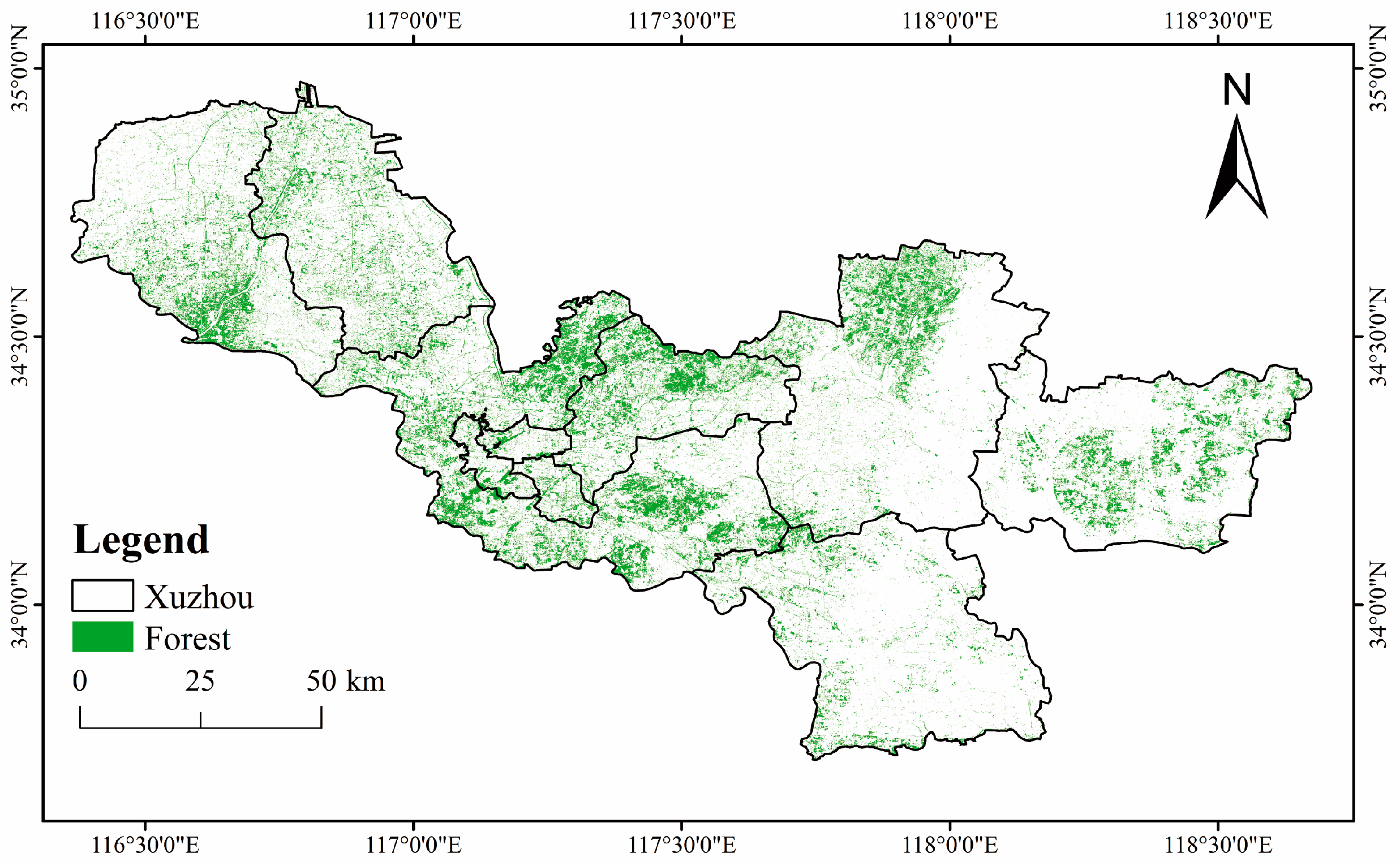
Since the below-ground biomass of vegetation is difficult to obtain, AGB is more commonly used to replace the traditional method for estimating biomass, which is to measure the weight of organic matter of all vegetation within a unit area in the field [10,11]. However, although the AGB of field measurements is more accurate, it requires a large amount of time and labor costs and causes damage to the survey object, it is difficult to use in large-scale AGB surveys [12]. Remote sensing is an effective technique for estimating AGB over large areas, which is characterized by a long number of observations, wide spatial coverage, multiple bands, and the ability to provide rich horizontal structural information [13]. Some studies have utilized a geographically weighted regression model (GER) [14], Random Forest model (RF), and other methods to establish the relationship between remote sensing image features and the samples of AGB in the field, and then invert the distribution of AGB in the whole image-covered area [15]. For example, Mthembeni Mngadi et al. and Sandra Eckert et al. used RF, multiple linear regression method with Sentinel-2 and WorldView-2 image data to invert the AGB distribution in the Buffelsdraai area, and in the northeast of Madagascar, respectively [16,17]. Jue Xiao et al. and Nichol et al. used the texture features to further improve the accuracy of AGB inversion from remote sensing images [18,19]. However, passive optical remote sensing images are unable to obtain vertical structural information of trees and are limited by the influence of cloud cover at the time of observation [20]. These limitations would result in the generally low accuracy of AGB estimation, especially in the dense vegetation areas with high biomass for the image spectra have a strong saturation effect and tend to lose sensitivity [21,22,23].
As an active remote sensing method, spaceborne Light Detection and Ranging (LiDAR) can penetrate the canopy to obtain three-dimensional structural information of vegetation in densely vegetated areas. The Global Ecosystem Dynamics Investigation (GEDI) instrument—a new-generation spaceborne LiDAR system from NASA—provides the first global coverage of high-resolution 3D altimetry data aimed specifically at mapping Earth’s forests [24]. LiDAR measurements of vertical forest structure are sensitive to higher AGB and have little or no saturation, which effectively improves the accuracy of the inversion of vegetation canopy height and AGB, and has been widely used in the estimation of AGB in forests, grasslands, and other large areas [25]. For example, Xiaohuan Xi et al. utilized the wavelet method and Geoscience Laser Altimeter System (GLAS) LiDAR data to invert the biomass distribution in Xishuangbanna, Yunnan Province, China [26]; Mengjia Wang et al. overcame the saturation at high values of the existing AGB map using a map of correction factors generated from GLAS spaceborne LiDAR data [27]. Carlos Alberto Silva et al. assessed data fusion framework using simulations of GEDI, ICESat-2, and NISAR data from airborne laser scanning (ALS) and UAVSAR data acquired over the temperate high AGB forest and complex terrain in Sonoma County, California, USA [28]. Since spaceborne LiDAR data are scattered and do not provide spatially continuous information, interpolation methods such as Kriging [29,30] or spatially continuous optical imagery [31] were used to generate a regional distribution of AGB [32,33]. These methods are suitable for the inversion of canopy height and AGB within large-scale forest regions [34,35,36,37], but it is a still challenge for the estimation of AGB in non-homogeneous areas such as urban areas. The distribution of vegetation in urban areas is scattered and diverse with strong spatial heterogeneity under the influence of human activities and dynamic land cover [38]. Spaceborne LiDAR footprints do not all fall right in the vegetation areas, and thus there is a certain inaccuracy in the estimation of AGB of vegetation in urban areas by directly using spaceborne LiDAR observations [39,40].
Considering that remote sensing imagery can obtain the complete spatial distribution of vegetation in the region, it is possible to establish the correlation between the features of vegetation extracted from the remote sensing imagery and height features of vegetation derived from the spaceborne LiDAR, and thus to estimate more accurate canopy height and AGB of vegetation in urban areas by combining spaceborne LiDAR data with remote sensing imagery. In this study, laser altimetry from GEDI and remote sensing multispectral imagery from Sentinel-2 and Landsat-8 satellites are combined to construct a coupling model between multi-parameter features of remote sensing imagery and the canopy height of vegetation derived from GEDI, and thus the canopy height and AGB of vegetation in all the region are estimated continuously and accurately. The city of Xuzhou in Jiangsu Province of China is selected as the study area to verify the effectiveness of estimating accurate canopy height and AGB of vegetation in the urban and neighboring areas.
The rest of this study is organized as follows. In Section 2, the study area and data used in this study are introduced. Section 3 is the methodology of vegetation canopy height extraction and AGB estimation using the combined data. The results of canopy height mapping and AGB estimation are described in Section 4. The discussion and conclusions are listed in Section 5 and Section 6, respectively.

2. Study Area and Materials

2.1. Study Area

As shown in Figure 1, the study area is located in Xuzhou City (116°22′~118°40′E, 33°43′~34°58′N), Jiangsu Province, which is situated in the eastern part of China and covers an area of about 11,258 km2. The topography of Xuzhou is dominated by plains with elevations generally ranging from 30 to 50 m above sea level, which account for about 90% of the city’s area. A few hills and mountains exist in central and eastern of Xuzhou, of which the elevation is generally about 100~200 m above sea level, and the area accounts for about 9.4% of the city. Affected by the southeast monsoon, Xuzhou has a temperate monsoon climate with four distinct seasons, no summer heat, no winter cold, plenty of sunshine, and moderate rainfall [41]. As an ancient coal city, Xuzhou has been transformed from a resource-depleted city into a national ecological garden city in recent years. The ecological environment has undergone great changes, especially the area of forest reaches about 288,567.62 hm2 and the forest coverage rate reaches about 27.8%, which is the highest forest coverage in the province [16]. Since Xuzhou is a well-developed city in central and eastern China, there are a lot of human activities in both urban and suburban areas, and the vegetation distribution is not uniform. It should be noted that different from the AGB estimation of only trees, three typical vegetated types in Xuzhou, the coniferous forest, broadleaf forest, and shorter vegetation, are selected to estimate the AGB. Because the shorter vegetation, including low crops in farmland, grass or shrubs, and scattered trees in residential areas takes up a lot of space, the whole administrative area of Xuzhou is selected as our study area.

2.2. Laser Altimetry Data

GEDI was launched on 5 December 2018, to collect data between 51.6°N and 51.6°S. During its nominal 24-month mission, GEDI has acquired approximately 10 billion cloud-free observations [42]. These data will be of immense value for forest and water management, carbon cycle science, and weather forecasting [43]. The GEDI instrument consists of three lasers emitting at a rate of 242 Hz, which produce eight parallel observation tracks that illuminate a 25-m diameter footprint on the surface of the 3D structure being measured [44]. The footprints are spaced 60 m apart in the same track and 600 m apart in the cross-track direction relative to the flight direction, with a cross-track width of about 4.2 km. It allows for high-resolution laser-ranging observations of the Earth’s 3D structure with the densest sampling of any LiDAR instrument to date. It provides an unprecedented sampling density of forest structural properties.
In this study, the L1B data of GEDI covering the study area in 2021 is selected to extract the canopy height of vegetation at the footprint level after the wave process described in Section 3.1. The data contains the corrected footprint data, and waveform data, which is available on (https://search.earthdata.nasa.gov/search (accessed on 27 March 2024)). Footprint data are geo-located with a position error of 15–20 m (standard deviation) and a ranging error of 0.6 m [42]. For each footprint, the parameters of waveform, waveform noise standard deviation, and waveform noise mean are selected to extract and calculate the canopy height of vegetation. The distribution of GEDI laser points is shown in Figure 1b. A total of 52,411 points are used in this study.

2.3. Optical Remote Sensing Imagery

To avoid the influence of clouds on images, two types of optical remote sensing imagery are selected. One is from the Sentinel-2 satellite, which is the primary image source for the extraction of spectral features and texture features. The other one is from the Landsat-8 satellite, which is only for extraction of spectral features.
Sentinel-2 is a high-resolution multispectral imaging satellite carrying a multispectral imager (MSI) at an altitude of 786 km, covering 13 spectral bands with a width of up to 290 km, which is used for terrestrial monitoring, providing images of vegetation, soil, and water cover, inland waterways and coastal areas, and also for emergency rescue services. From visible and near-infrared to short-wave infrared with different spatial resolutions (10 m, 20 m and 60 m). Sentinel-2 data is the only data type among the optical data types that contains three bands in the red-edge range, which is very effective for monitoring information on vegetation [45]. We downloaded Sentinel-2 images from ESA (https://browser.dataspace.copernicus.eu/ (accessed on 27 March 2024)) (Figure 1b) and chose images with less than 10% cloudiness to meet the quality requirements.
Landsat-8 carries two sensors, the OLI (Operational Land Imager) and the TIRS (Thermal Infrared Sensor) [46]. The spatial resolution of these images is 30 m, and the projection system of these images is Universal Transverse Mercator (UTM) (World Geodetic System (WGS) 84 datum) [47]. These multi-temporal Landsat-8 images cover different vegetation states from green to dormant, which has great flexibility for a wide time span and many options. We download these images from the USGS website (https://earthexplorer.usgs.gov (accessed on 27 March 2024)). Images with less than 10% clouds acquired at different times but in the same season are used as a priority. The image information is shown in Table 1.

2.4. Digital Elevation Model (DEM) Data

DEM from the Shuttle Radar Topography Mission (SRTM) is also selected as one surface feature to estimate the AGB in this study. SRTM was executed by NASA and the National Geospatial-Intelligence Agency (NGA) in 2000. The 11-day mission was used to generate near-global land elevation data products. SRTM successfully collected elevation data over 80% of the Earth’s surface (60°N–56°S) and ultimately acquired a global digital elevation model (DEM) with a planimetric accuracy of ± 20 m and elevation accuracy of ±16 m. In this paper, the elevation values of the DEM data covering the study area with a spatial resolution of 30 m were downloaded from the U.S. Geological Survey website (https://earthexplorer.usgs.gov (accessed on 27 March 2024)).

2.5. Measurements from Fieldwork

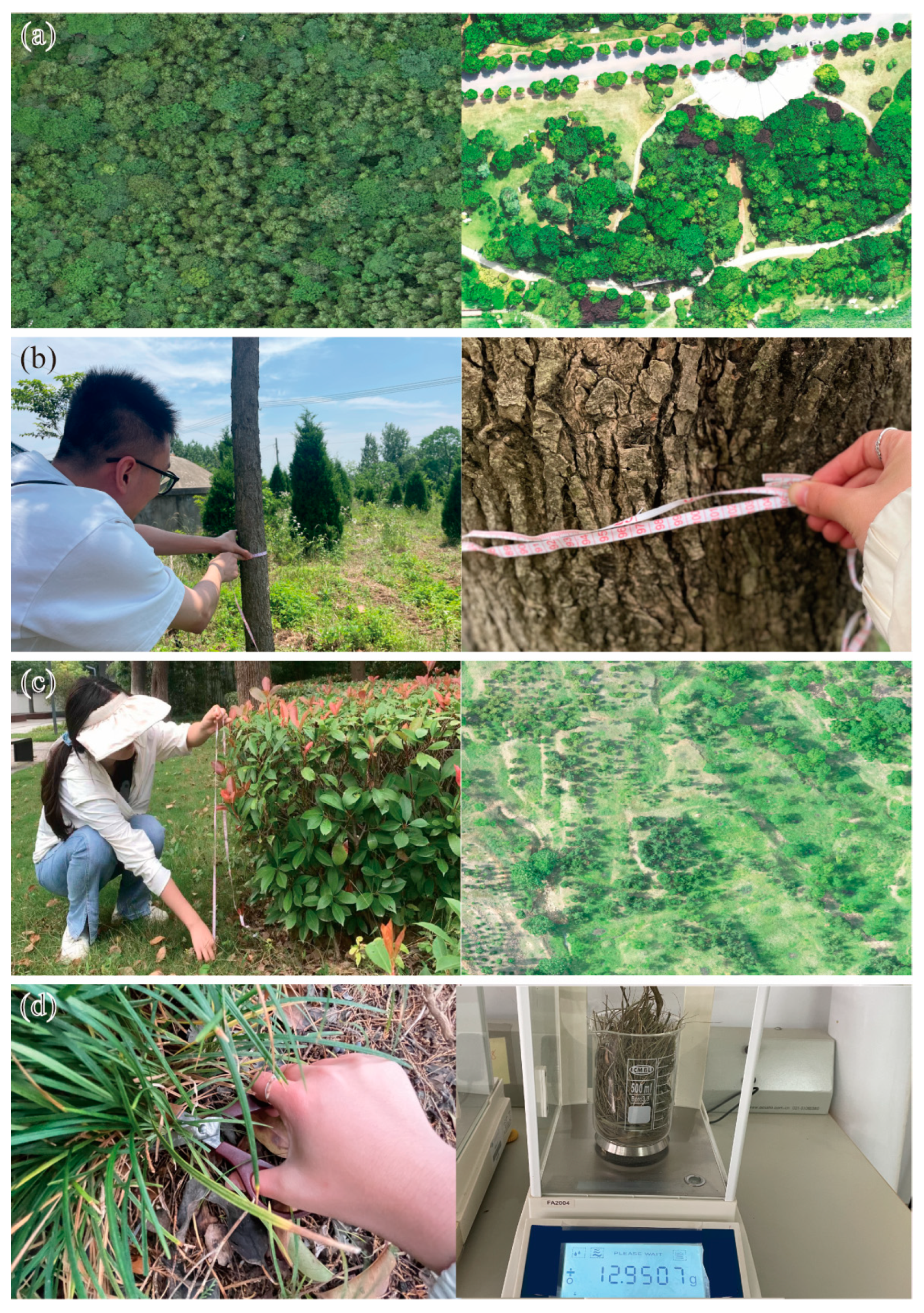
The canopy height and AGB of vegetation obtained by field measurements are used to validate the accuracy of AGB estimation of vegetation in this study. The quadrat is set as an area of interest (25 m × 25 m circle) in different vegetated areas, where there are laser observations according to the distribution of GEDI footprints. The quadrats with different vegetation cover are as evenly distributed as possible and surveyed by unmanned aerial vehicles (UAVs) or manual measurements. There are 22 field measurement quadrats in this study.
For the forest area, UAVs are used to obtain the tilted images of the area. The images are performed by 3D modeling to obtain the canopy height of the forest. At the same time, a laser range finder is supplemented to measure the canopy height of the trees, and a tape measure is used to measure the diameter at the breast height (DBH) of all the trees in the area. For the area with scattered vegetation distribution, the total number, canopy height, and DBH of trees are measured. For the area where the vegetation type is shorter vegetation, such as crops or shrubs in Figure 2c, a tape measure is used to obtain their heights, and above-ground vegetation per unit area is cut close to the ground and brought back to the laboratory, dried in a dryer, and weighed on an electronic balance for AGB calculations as shown in Figure 2d. There are 13 samples with shorter vegetation in this study.

3. Methods

In this study, the inversion of AGB in urban areas combines the advantages of vegetation canopy height obtained from laser altimetry data with the advantages of spatially continuous distribution of vegetation extracted from optical images. In the area covered by vegetation and also distributed by GEDI footprints, a correlation model is established between the vegetation canopy height obtained from laser altimetry and multi-features extracted from optical images. Based on this model, the vegetation canopy height in other areas without GEDI distribution can be estimated. Then, the AGB of vegetation is estimated by combining the vegetation canopy height and vegetation classification information.
The specific method consists of five steps: (1) Process the GEDI waveform data to obtain canopy height; (2) Extract a series of spectral, textural, and elevation parameters from optical images; (3) Establish a correlation model between vegetation canopy height and multi-features from optical images and DEM parameters in the vegetation coverage areas with GEDI footprints distribution; (4) Generate spatially continuous vegetation canopy heights in all vegetation cover areas and evaluate the accuracy of vegetation canopy height maps; (5) Combine the vegetation canopy height and vegetation type to invert the spatially continuous AGB maps and evaluate the accuracy of AGB. The flow chart of the method is shown in Figure 3.

3.1. Canopy Height Extraction from GEDI Waveform Data

The canopy height is equal to the elevation difference between the elevation of vegetation and the bare elevation of the ground, which corresponds to the start of the laser signal corresponding to the echo minus the elevation corresponding to the ground echo, as shown in Equation (1) [48].
Canopy height = Signal_start − Ground_return
To ensure the high quality of the training and validation data, the available GEDI waveform data with beam sensitivity ≥ 0.95 are selected. Beam sensitivity is a measure of signal-to-noise related to the canopy cover through which a waveform has sufficient energy to penetrate the ground [48].
Due to signal saturation and natural conditions, the quality of waveform data will be reduced, so the original data should be pre-processed before the forest canopy height is obtained to ensure the accuracy of waveform parameters and canopy height extraction. The main contents of waveform data processing include data normalization, Gaussian filtering, noise estimation, threshold determination, ground echo, and canopy echo location determination [49].
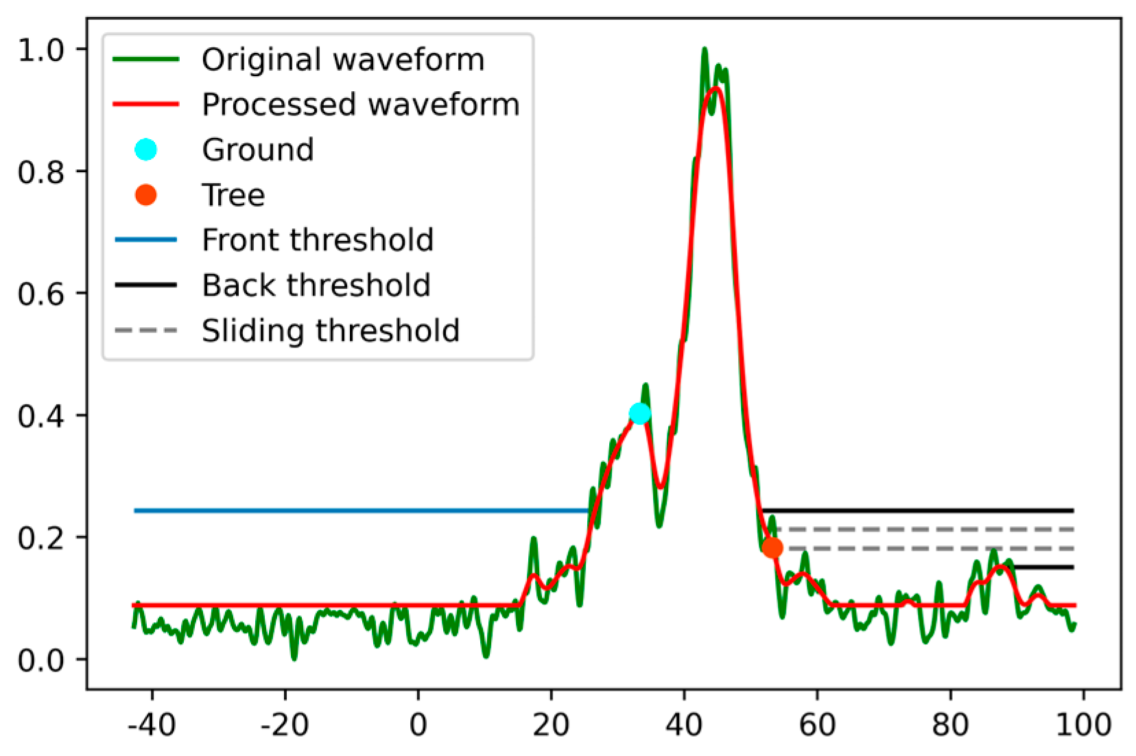
First, the GEDI waveform amplitude is standardized to the range 0~1 as the normalized cumulative return energy, and the standardized waveform is shown as the green curve in Figure 4; Then the Gaussian filtering is performed on the standardized waveform so that the waveform is smoothed, and the processed waveform is shown as the red curve in Figure 4; The waveform length is defined as the vertical distance between the first effective return (Signal_start) and the ground return (Ground_return) in the Gaussian-filtered smoothed waveform as shown in Equation (1).
The first valid echo is defined as the rightmost intersection of the post-threshold with the normalized smooth waveform (orange point in Figure 4), and the ground echo is defined as the peak Gaussian component on the last valid echo with the peak Gaussian greater than the pre-threshold (blue point in Figure 4). The canopy height is equal to the elevation corresponding to the first valid echo minus the elevation corresponding to the ground echo.
To determine the thresholds, the average noise and the noise standard deviation are used. The thresholds include the pre-threshold and post-threshold. The pre-threshold is used to extract the canopy height, while the post-threshold is used to extract the ground elevation. These thresholds are calculated using different constants, which can be found in Equation (2):
h0 = h1 ± x × h2
where h0 is threshold, h1 is the average noise, h2 is the noise standard deviation, x is constant, and x are different constants to obtain the pre-threshold and post-threshold, respectively.
The method of sliding threshold is used to test the extracted canopy height. When the canopy height is greater than the average of all canopy heights plus 5 times the standard deviation of the canopy heights, the post-threshold is continuously increased to re-extract the canopy heights until the post-threshold is equal to the pre-threshold. If the canopy height is not greater than the average of all canopy heights plus 5 times the standard deviation of the canopy heights in the process of increasing the post-threshold extraction, the canopy height under the threshold is directly output as the new canopy height. If in the process of increasing the post-threshold extraction, until the post-threshold is equal to the pre-threshold, the canopy height is still greater than the average of all canopy heights plus 5 times the standard deviation of the canopy height, it means that the data are accurate, and still outputs the canopy height under the most original threshold.
We check whether the extracted canopy heights are too large due to the influence of noise by continuously increasing the post-threshold, which means that the location of the canopy echoes is checked to avoid overestimation of the canopy height. The blue straight line in Figure 4 is the pre-threshold (the noise mean + 5.5 × noise standard deviation), the black straight line is the post-threshold (the noise mean + x × noise standard deviation), x takes the value of 3~5.5, and the short gray line is the sliding post-threshold.

3.2. Feature Extraction from Optical Images in Vegetated Areas

Features including spectral indices, vegetation indices, texture, topography, seasonal characteristics, and land type are extracted to describe the characteristics of vegetated areas. Spectral indices include spectral values in the vegetated area, vegetation indices include normalized difference vegetation index (NDVI), green normalized difference vegetation index (GNDVI), enhanced vegetation index (EVI), normalized burn ratio (NBR), relative vigor index (RVI), difference vegetation index (DVI), atmospherically resistant vegetation index (ARVI). A texture feature is a global feature that describes the surface properties of the image region, including the parameters of Mean, Variance, Homogeneity, Contrast, Dissimilarity, Entropy, Angular Second Moment, and Correlation. We use ENVI 5.6 for texture feature extraction, and the specific parameters are shown in Table 2. Texture features, vegetation indices, and spectral indices are extracted for Sentinel-2 imagery, while vegetation indices and spectral indices are extracted for Landsat-8 imagery after performing radiometric calibration and atmospheric correction. In addition, surface topography parameters are extracted from SRTM. The extracted parameters for the vegetated area are shown in Table 2.
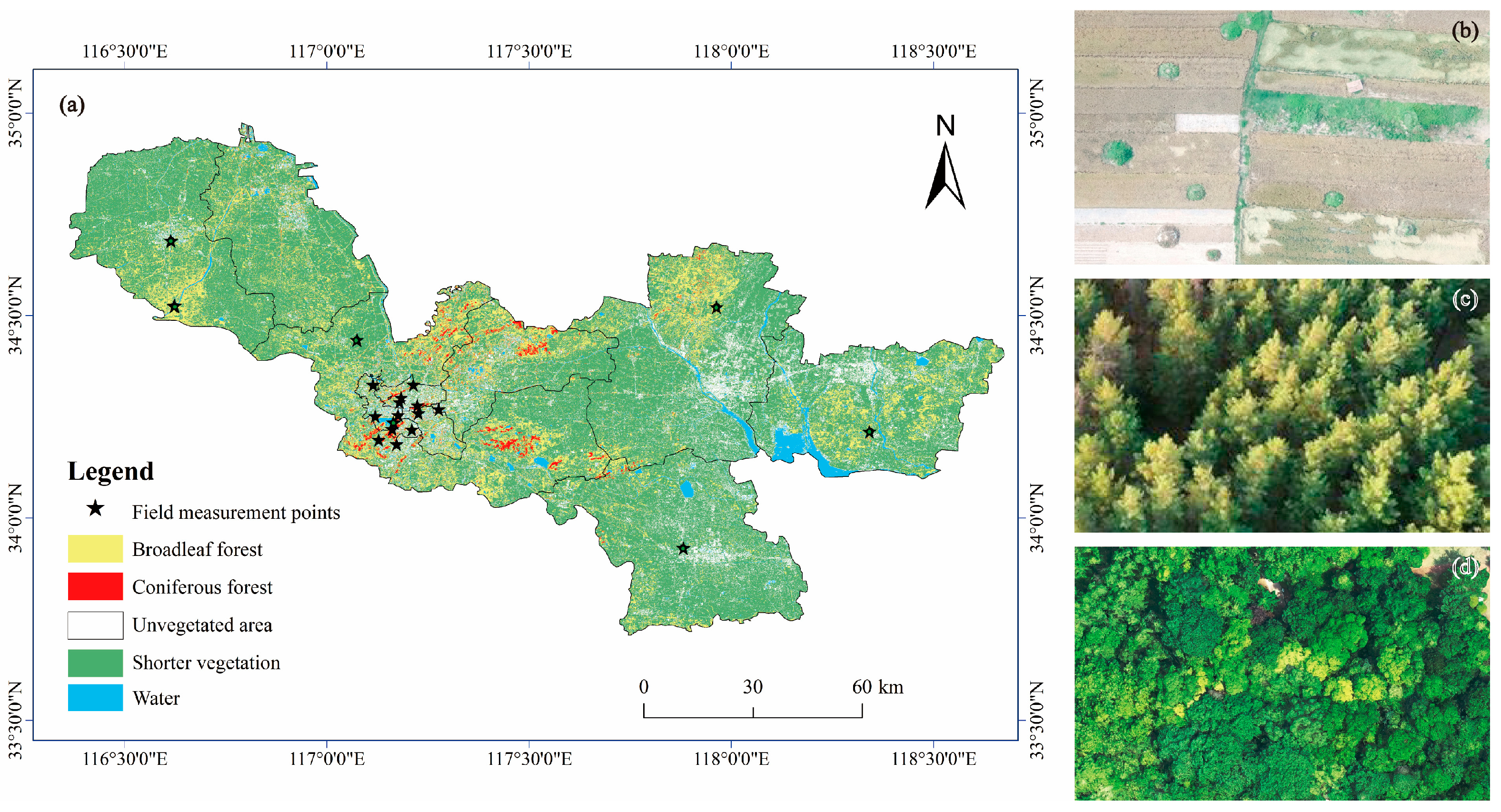
Sentinel-2 imagery and Landsat-8 imagery in 2021, according to the timing of GEDI observations, are used to extract the vegetated area. Since the vegetation growth is strongly tied to seasonal changes, images in four seasons are considered and processed separately. The images with clouds are removed and replaced by images taken on similar dates. Support vector machine classification method based on false-color images and the field investigation is adopted to generate the region-of-interest samples and classification. As shown in Figure 5, the land cover in Xuzhou is divided into five types in this study, unvegetated area, water, coniferous forest, broadleaf forest, and shorter vegetation, which are covered with low crops or shrubs, or scattered trees in residential areas. The coniferous forest, the broadleaf forest, and the shorter vegetation region are selected as the vegetated area and used for AGB calculation in this study.

3.3. Canopy Height Estimation Model through Random Forest

3.3.1. Canopy Height Estimation Model Using GEDI Joint Optical Images

To estimate the vegetation canopy height in all vegetated areas, Random Forest (RF) is adopted to establish the correlation model between the vegetation canopy height and feature parameters of the vegetated area extracted from optical images. In the vegetated areas with GEDI observations, the canopy height of vegetation is extracted from GEDI using the method in Section 3.1. Assuming that the canopy height extracted from GEDI in vegetated areas is h , the corresponding feature vector in this vegetated area is X , then the correlation model can be described in Equation (3):
h = f ( X )
where X = [ x 1 , x 2 , , x 43 ] , representing 43 feature parameters of vegetated area. The spectral indices from each band of the multispectral optical image, eight texture features, and seven vegetation indices in Table 2 are denoted as x 1 , x 2 , …, x 39 . The slope and elevation parameters are denoted as x 40 and x 41 , respectively. The quarterly information is denoted as x 42 , and the land cover of the region is denoted as x 43 . The RF algorithm is used to establish the nonlinear relationship model between the independent variable X and the dependent variable h for its high tolerance for noise and outliers, which can avoid the problem of overfitting [55]. Since the RF algorithm is based on decision trees, it has two important parameters, the maximum depth in the tree (mdep) and the number of trees (ntree). In this study, the values of mdep and ntree are set to 30 and 100, respectively. X is the input in the RF model to predict the canopy height h . Therefore, with the correlation model, the vegetation canopy height can be estimated using the feature parameters extracted from optical images in all vegetated areas.
It should be noted that a uniformly distributed grid with a spatial resolution of 300 m is established in the study area. All the feature parameters are extracted for each pixel of the grid in the vegetated area and used as inputs in the RF model to predict canopy height for each pixel. The average value of the points falling in the grid is taken as the canopy height of the grid to generate a spatially continuous canopy height map covering the study area.

3.3.2. Canopy Height Estimation Model Only Using Optical Images

Assuming that the canopy height extracted by the UAV is Z and the feature vector corresponding to this vegetation zone is the above X , the correlation model can be described by Equation (4):
Z = f ( X )
The optical image inversion of canopy height is performed in the same way as the method described above, while the RF model and X are trained by the canopy height Z acquired by the UAV. Therefore, with the RF model, the vegetation canopy height can be estimated using optical images in all vegetated areas.

3.4. Estimation of AGB with Canopy Height of Vegetation

For the estimation of AGB within the field samples, the stratified aggregation method is used to calculate the AGB of the tree, shrub, and grass layers separately, then summed to obtain the total AGB. To derive the AGB of the vegetation in this area on an individual tree basis, the canopy height, tree DBH, and crown width are measured in the field. These measurements are used in conjunction with allometric growth equations to establish a model for the maximum canopy height and AGB (refer to Equation (5)).
AGB = F (Max (Canopy height))
where F can be in the form of power function, exponential function, etc. (Table 3). By comparing the field measurement of AGB with the inversion results, the power function model with the highest accuracy is selected as the final AGB estimation model. This equation derives the spatially continuous AGB map by bringing into the canopy height from the spatially continuous canopy height map.

4. Results

4.1. Vegetation Canopy Heights Mappings

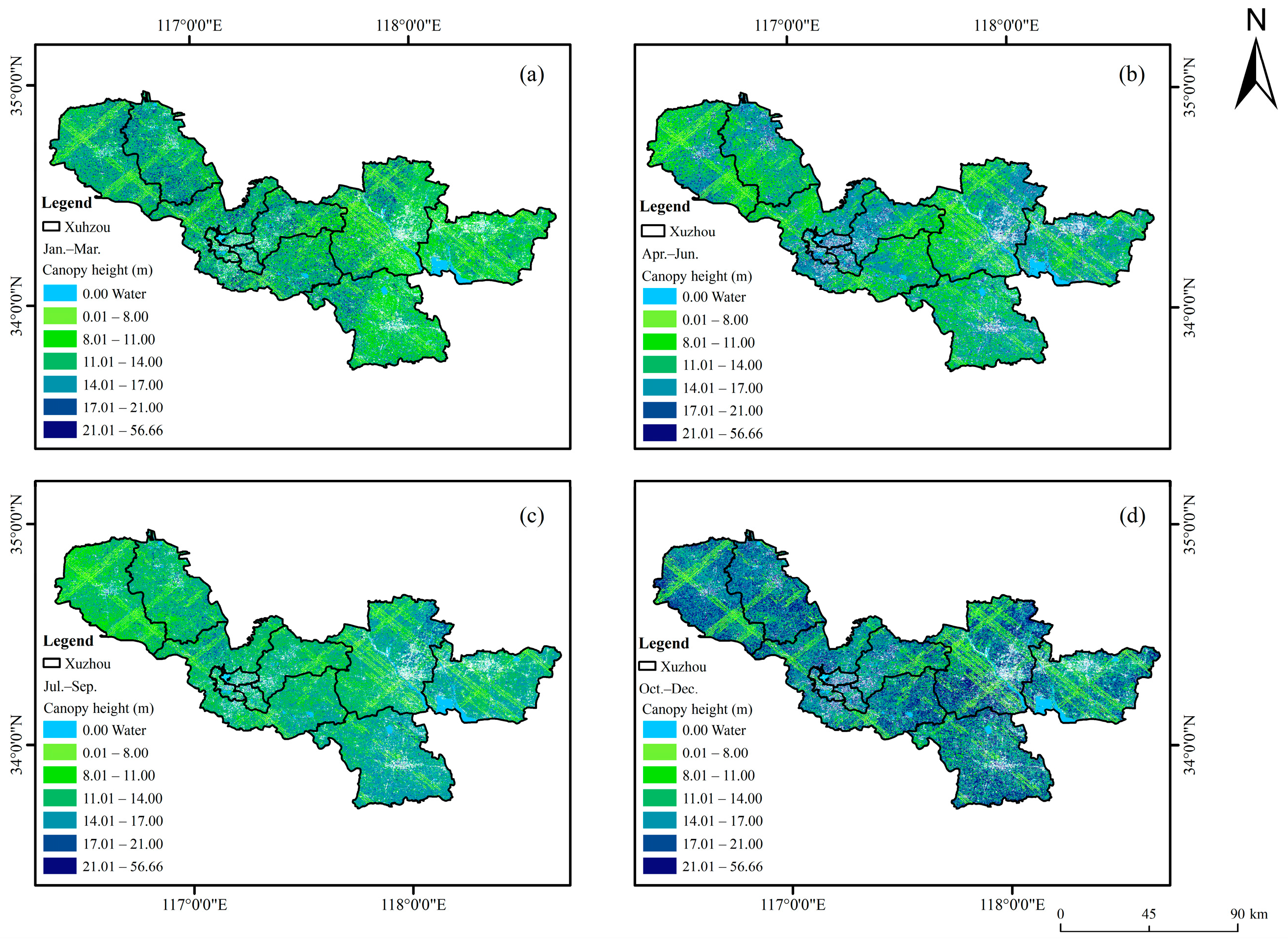
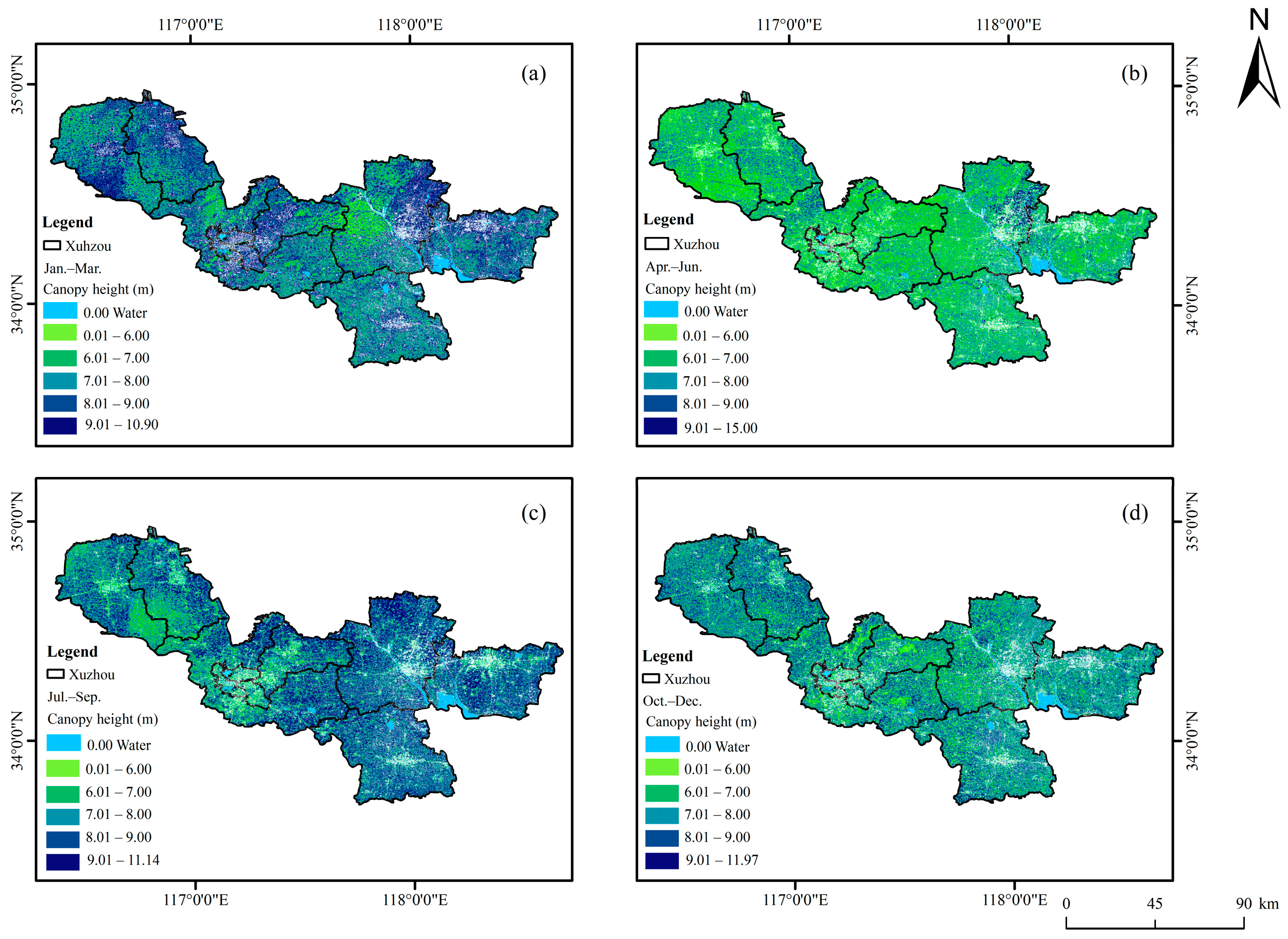
The continuous canopy height map inverted by GEDI joint optical imagery is shown in Figure 6. Figure 6a–d show the canopy height maps for January–March, April–June, July–September, and October–December, respectively. Since the vegetation canopy height extracted by GEDI has the highest accuracy, it is used in fishnets with GEDI footprints, and the vegetation canopy height estimated by GEDI joint optical imagery inversion is used in fishnets without GEDI footprints. The average canopy height at 17.77 m. The northwest, northeast, and central parts of the study area showed higher canopy height, mainly ranging from 17 m to 56 m. The canopy height in the other regions is relatively low, mainly ranging from 0 to 12 m, corresponding to the shorter vegetation regions. The canopy height during the months of July–September are obviously relatively lower, while those in the months of October–December are obviously higher.

4.2. Vegetation AGB Mappings

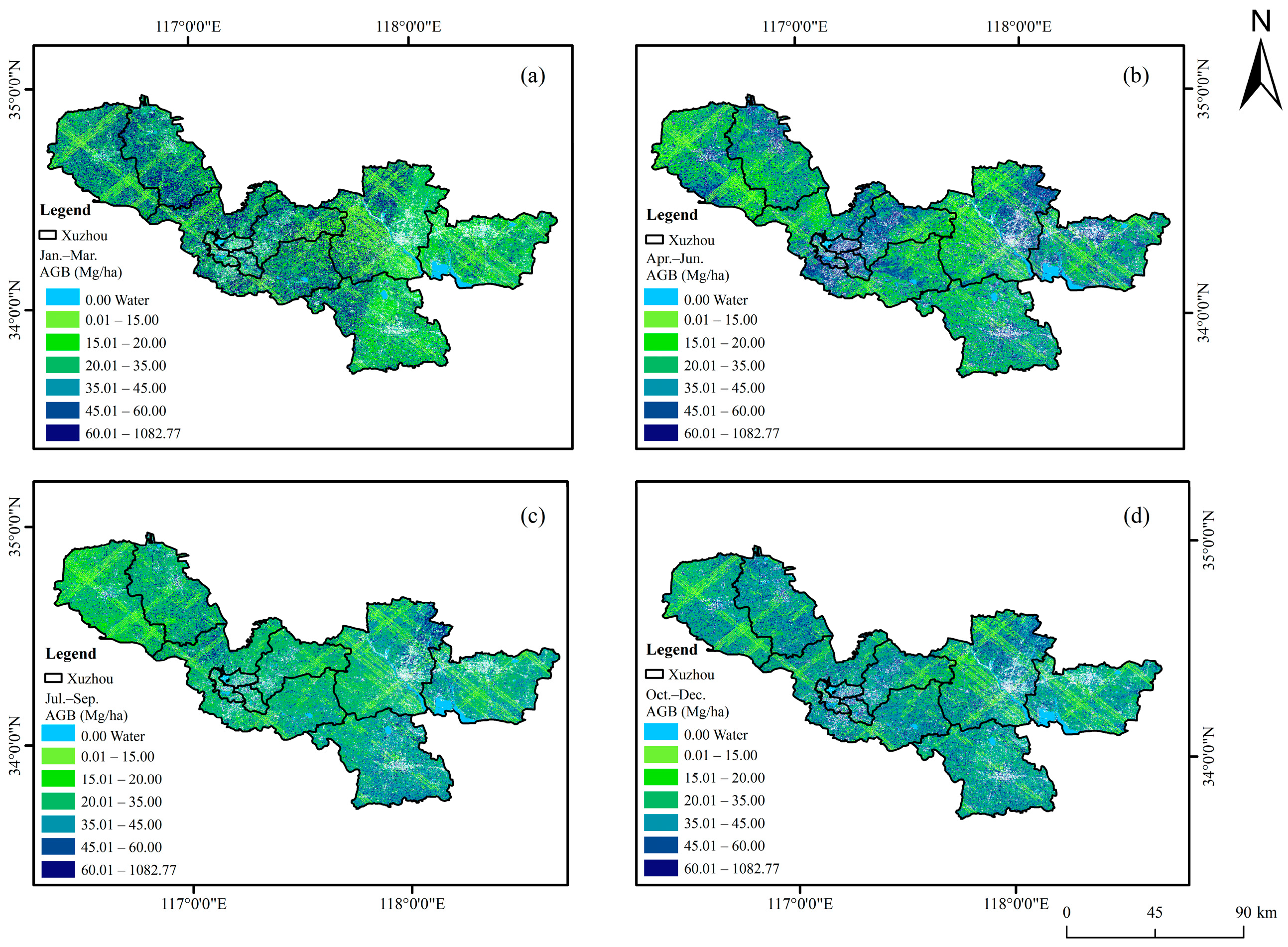
The results of the canopy height values from the inverse GEDI joint optical images are substituted into the power function for AGB estimation. Then, the AGB values are obtained in a spatially continuous manner. Figure 7a–d show the AGB maps for January–March, April–June, July–September, October–December, respectively. As can be seen in Figure 7, the distribution of AGB is similar to that of canopy height.

4.3. Comparison and Validation

4.3.1. Canopy Height Accuracy

The canopy heights obtained from the UAV modeling are taken as the true values to evaluate the canopy height accuracy of optical image inversion. The spectral index, land class information, etc. of the spot are extracted to estimate the canopy height using RF modeling 70% of the UAV modeled canopy height is divided into a training set and 30% into a test set. Figure 8a shows the validation of the accuracy of the inverted canopy height of the optical imagery with the canopy height extracted from the three-dimensional modeling of the UAV imagery (R2 = 0.59, RMSE = 2.23 m).
However, the accuracy is mostly validated by the canopy heights extracted by GEDI. Figure 8b shows the accuracy validation of the canopy heights extracted by GEDI against the canopy heights predicted by GEDI joint optical imagery using the RF method (R2 = 0.94, RMSE = 1.59 m).
The continuous vegetation canopy height map from the GEDI joint optical images inversion is shown in Figure 6 and the continuous canopy height from the optical image inversion is shown in Figure 9. It is observed that the canopy height range of the optical image inversion is limited, leading to singular values in the inverted canopy height due to incomplete sample coverage.
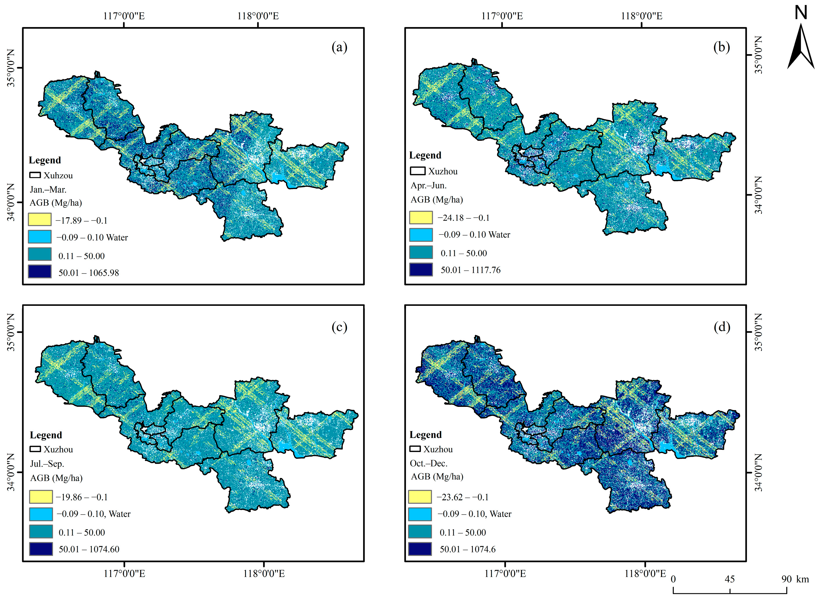
Figure 10 shows the difference obtained by the vegetation canopy height from GEDI joint optical images inversion minus the vegetation canopy height from optical images inversion. The blue part is water, there is no vegetation in the water, so there is no change in canopy height. Except for the strip areas with GEDI footprints, the canopy height of vegetation estimated by GEDI joint optical images is significantly higher than that only by optical image inversion. This is due to the fact the inversion of vegetation canopy height with optical imagery needs more samples and more comprehensive coverage in the study area.

4.3.2. AGB Accuracy

Four fitting functions including the cubic term function, power function, exponential function, and quadratic function are tested for the relationship between max canopy height and AGB derived from partial field measurements. According to the distribution of vegetation canopy height in Figure 6, most of the vegetation canopy heights in Xuzhou are less than 20 m, nine field measurements with canopy height less than 20 m are used as the sample sites to fit the model, the remaining field measurements are used as the validate data.
Figure 11 shows the results of four fitting functions. The AGB measured fitting model performed best with the cubic term function (Figure 11a), but there is overfitting. The power function (Figure 11b) with fitting value R2 = 0.80, RMSE = 8.10 Mg/ha performed better and more accurately than others, so the power function is adopted to predict the values of AGB in the subsequent study.
Figure 12a is the comparison between the measured AGB and the predictions of AGB obtained by joint inversion of GEDI observations and optical images, and the fitting value R2 = 0.58, RMSE = 14.25 Mg/ha. Figure 12b is the comparison between the measured AGB and the predictions of AGB obtained only by optical images, and the fitting value R2 = 0.45, RMSE = 13.55 Mg/ha. It is apparent that the joint estimation using GEDI and optical images results in higher accuracy in AGB inversion than that using only optical images.
Figure 13 shows the difference obtained by the AGB from GEDI joint optical images inversion minus the AGB from optical images inversion. It can be seen that the distribution of AGB in Figure 13 is the same as the distribution of canopy height in Figure 10.

5. Discussion

5.1. Importance of Multi-Features for Canopy Height and AGB Estimation

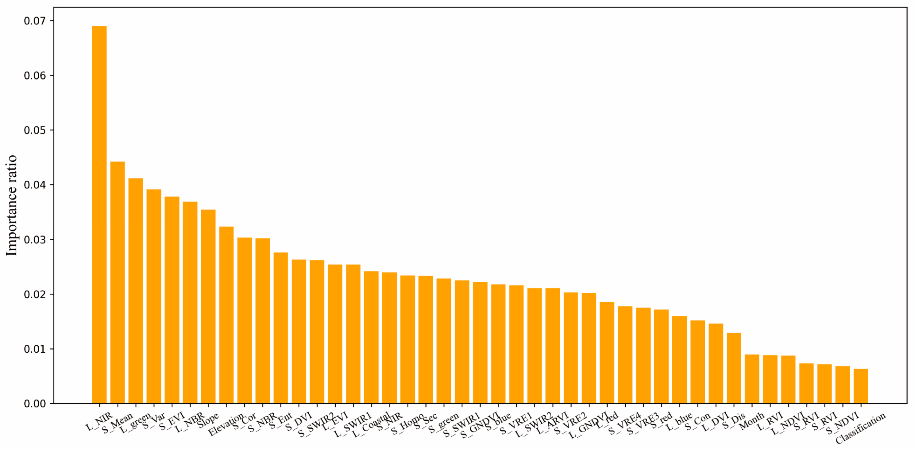
Figure 14 shows the importance of each feature parameter, which is calculated by averaging the estimates of predictive values over several randomized features in RF. The higher the reduction of the variance of such an estimate, the more important the contribution of the matching feature. The total importance ratios of all features are positive and sum to 1.0. It can be seen that the NIR band of Landsat-8 images had the strongest influence on predicting canopy height, followed by texture features of Sentinel-2 imagery. Moreover, the key spectral variables for canopy height estimation are EVI and NBR, which are both closely correlated with the NIR band. However, other vegetation indices like NDVI and RVI, had low correlations with canopy heights. The reason for this is that the vegetation indices are not likely to perform well in dense forests with complex structures because of saturation problems and shadow effects of the tall trees [65]. Topographic parameters including slope and elevation also have a high impact on the estimation. This may be because the height of vegetation is affected by terrain, and the extraction of bare terrain requires more consideration.
On the other hand, textures extracted from Sentinel-2 images show greater potential for canopy height estimation. Texture features can enhance the discrimination of spatial information and canopy detection levels simultaneously, something that cannot be achieved with spectral vegetation indices [19]. Textures extracted from images with medium-to-high spatial resolution are also capable of simplifying complex canopy structures and have a strong correlation with forest stand structure, including density, age, and leaf area index [18].
Moreover, As shown in Figure 10b, the optical image inversion of vegetation canopy height is significantly underestimated, especially in the coniferous forest area (Figure 5a). This is because the near-infrared radiation from remote sensing cannot penetrate the canopy, and the spectral parameters can only obtain the canopy height of the vegetation, but not detailed information about its structure. However, the canopy of trees and shrubs is very similar to the optical images, thus leading to a lower estimation of the more heavily wooded and taller areas and a higher estimation of the places with shorter vegetation.

5.2. The Impact of Vegetation Distribution on AGB

The value of AGB is closely related to the distribution and type of vegetation [66]. Table 4 lists the AGB distribution with GEDI joint optical images in Apr.-Jun. The area of shorter vegetation region, broadleaf forest, and coniferous forest is 754,389 ha, 168,768 ha, and 19,404 ha, respectively. Compared with the distribution of vegetated areas in Figure 5, the total AGB in the shorter vegetation region is the highest because it has the largest coverage area in Xuzhou, while the total AGB of the coniferous forest is the lowest. However, the lowest AGB per unit area of 33.60 Mg/ha is found in the shorter vegetation region. Since the broadleaf trees are often sporadic distributed in the shorter vegetation region, the AGB per unit area of the broadleaf forest is about 34.76 Mg/ha, which is similar to that in the shorter vegetation region. The coniferous forests shown in Figure 5a are mostly distributed in the mountains or forest parks, where trees are concentrated and dense. Therefore, the AGB per unit area of coniferous forest is the largest, with 46.60 Mg/ha.
Meanwhile, the ratios of AGB distribution from different vegetated areas in Xuzhou are plotted in Figure 15. The ratio of AGB per unit area between 0 and 40 Mg/ha is about 67.0% in the shorter vegetation region in Figure 15a, while it is only 20.7% in the coniferous forest in Figure 15c. On the contrary, the ratio of AGB per unit area above 40 Mg/ha is about 79.3% in the coniferous forest which is larger than that only 33.0% in the shorter vegetation region. It can be seen that coniferous forests have a wider distribution range of AGB per unit area.
It can be seen that the contribution of the shorter vegetation region plays an important role in the AGB in Xuzhou, as its coverage is much larger than that of the coniferous and broadleaf forests. However, most AGB estimations of shorter vegetation are more concentrated in local small areas of farmland dominated by a single crop [8]. Therefore, the estimation of AGB in the shorter vegetation region should be equally emphasized in future studies.
Figure 16 shows the distribution of forests in Xuzhou, including both coniferous and broadleaf forests in Figure 5a. Compared with the distribution of AGB in Figure 7, the areas with more AGB are mostly distributed in urban forests. Compared with grass ecosystems, forests have a longer life cycle, a fairly complex hierarchy, higher AGB and growth, etc. [67]. The range of AGB in urban forest regions is significantly higher than in shorter vegetation regions. Because the urban unvegetated area is mostly covered by impervious surfaces such as roads, buildings, etc., vegetated areas patches are mostly fragmented and have high landscape heterogeneity when compared to the large dense forests. More detailed classification and extraction of vegetated areas should be considered in the estimation of AGB or carbon for urban regions.

5.3. Seasonal Factor for the Estimation of Canopy Height and AGB

The AGB distribution is also different in different seasons [15]. Since the inversion of AGB is directly related to the canopy height of vegetation obtained by GEDI joint optical images, the variation of AGB corresponds to the variation of vegetation canopy height in different seasons. Table 5 lists the average AGB in different seasons using GEDI joint optical images.
As shown in Table 5, the highest AGB per unit area is highest in October–December and lowest in July–September in Xuzhou. July–September is the hottest time with lush vegetation growth and green foliage in Xuzhou. However, the denser leaves block the information on tree density, a forest attribute directly related to AGB at stand level [10]. The sparse laser points cannot fully consider the denser leaves in this season, which leads to the lower estimation of the canopy height of vegetation in Figure 6c; thus the AGB is underestimated, which is about 30.95 Mg/ha. At the same time, the shorter vegetation is very similar to trees in the optical images due to the saturation effect, which leads to the higher estimation of the canopy height of vegetation using only optical images as shown in Figure 9c. It means that a more accurate estimation of AGB calls for more laser observations or more field measurements.
On the other hand, October–December is the harvesting season in Xuzhou, the green leaves of the vegetation start to fall off in this season. The inversion of vegetation canopy height using only optical images is strongly influenced by spectra. The shedding of leaves of shrubs and trees results in an overall underestimation of vegetation canopy height in Figure 9d. In contrast, shorter vegetation regions and trees can be well differentiated using GEDI joint optical imagery, and the influence of the saturation effect is limited during this season. Therefore, higher vegetation canopy height and AGB occur in October–December as shown in Figure 6d and Figure 7d, which has the largest AGB of 59.55 Mg/ha.
Figure 17 shows the difference in the GEDI joint optical imagery inversion of the AGB between October–December and April–June. It can be seen that the estimation of the AGB would decrease during the time when the vegetation is flourishing. As shown in Figure 7b, AGB levels are more average in April–June. There are more AGB in October–December than that in April–June on the whole, especially in the region with shorter vegetation. As shown in Table 5, the AGB per unit area in the shorter vegetation region is 59.70 Mg/ha in October–December, while it is only 33.59 Mg/ha in April–June. This is due to the fact that October–December is the harvesting season for rice in Xuzhou, whereas April–June is the sowing season for rice. Therefore, the AGB in the shorter vegetation region is higher in October–December than that in April–June.
In addition, most of the red areas in Figure 17 are residential areas, and the region in the red ellipse is the main urban area of Xuzhou, where vegetation types are diverse and dispersed, which also leads to a large difference in the estimated AGB values. However, there is little difference in the water area or the GEDI strips, because there is litter vegetation in the water and the canopy height of vegetation observed by GEDI is not much affected by the season factors.

5.4. Influence of Field Measurements on AGB Estimation

The field measurements were collected between April and October 2023, while the images involved in the AGB inversion were acquired in 2021. This temporal mismatch between field measurements and participating datasets likely contributes to increasing the uncertainty of the results [68]. To match the location of the laser footprints of GEDI, all the field samples need to fall in the area with laser footprints. Although the 22 field samples are evenly distributed in the study area, the number of sampling quadrats is still insufficient for the whole large area, which leads to possible uncertainties in the modeling of canopy height and AGB of vegetation, especially the reference of AGB.
At the same time, it is not convenient to collect or measure the AGB of all the local vegetation directly, the AGB in the forest samples is measured by an allometric equation, which would also lead to uncertainties in the inversion of AGB [69]. This is because the AGB of vegetation is different in different areas even with the same vegetation. The allometric growth equation of the sample trees in this study refers to that of relevant trees in China, a more accurate AGB reference in Xuzhou should be considered and obtained to optimize the estimation model.

6. Conclusions

In this study, GEDI laser observations joint Landsat-8 and Sentinel-2 imagery are utilized to estimate the canopy height of vegetation and thus the AGB in Xuzhou. The correlation between the discrete vegetation heights of GEDI observations and multi-features extracted from optical images is constructed using Random Forest (RF) to obtain the vegetation canopy heights in all vegetated areas, thus estimating the AGB in all study areas. The conclusions of the study are summarized below:
(1)
The method of combining GEDI and optical images can improve the accuracy of vegetation canopy height estimation, and thus effectively improve the accuracy of AGB estimation. The estimation accuracy (R2 = 0.58) is higher than that of using only optical images (R2 = 0.45).
(2)
Three typical vegetated areas including the coniferous forest, broadleaf forest, and the shorter vegetation region are extracted to estimate the AGB. The total AGB in the shorter vegetation region is higher than the other two in the broadleaf forest and the coniferous forest, but the AGB per unit area is the lowest in the shorter vegetation area at 33.60 Mg/ha, and the coniferous forests have a wider distribution range of AGB per unit area at 46.60 Mg/ha.
(3)
Seasonal variations in vegetation also have a significant impact on the estimation of AGB. However, the highest average AGB occurs in October–December at 59.55 Mg/ha in Xuzhou using GEDI joint optical images, which is different from the normal pattern and the results using only optical images. A more accurate estimation of AGB calls for more laser observations or more field measurements.
(4)
The importance of multi-features is different for canopy height and AGB estimation. The near-infrared band and texture features have a greater influence on the estimation. However, the spectral similarity of trees and shrubs in the optical images leads higher estimation of canopy height in the shorter vegetation region and lower estimation in forest areas while using GEDI joint optical images. More detailed structures and precise features of vegetation are needed for AGB estimation in the future.
Vegetated areas are an important part of the urban ecosystem and play an important role in improving the quality of life and regulating the climate. In general, trees have a greater capacity to sequester carbon and produce more AGB than shorter vegetation. However, it is crucial to diversify tree species to reduce ecological vulnerability and ensure stronger urban ecosystems, leading to more sustainable urban development. Although large-scale mapping can be realized by inverting AGB with heterogeneous growth equations, the accuracy still needs to be improved. Additionally, the structure and composition of urban trees are more complex than natural forests, and the estimation of urban biomass is still subject to large errors due to the heterogeneity and fragmentation of urban landscapes and needs more consideration.

Author Contributions

Conceptualization, W.H. and X.Z.; methodology, X.Z.; software, X.Z.; validation, J.X., J.H. and W.W.; formal analysis, W.H.; investigation, J.H.; resources, W.W.; data curation, W.H.; writing—original draft preparation, X.Z.; writing—review and editing, W.H.; visualization, X.Z.; supervision, W.H.; project administration, W.H.; funding acquisition, W.H. All authors have read and agreed to the published version of the manuscript.

Funding

This research received no external funding.

Data Availability Statement

The raw data supporting the conclusions of this article will be made available by the authors on request.

Conflicts of Interest

The authors declare no conflict of interest.

References

  1. Wilson, J.S.; Clay, M.; Martin, E.; Stuckey, D.; Vedder-Risch, K. Evaluating environmental influences of zoning in urban ecosystems with remote sensing. Remote Sens. Environ. 2003, 86, 303–321. [Google Scholar] [CrossRef]
  2. Pataki, D.E. Urban greening needs better data. Nature 2013, 502, 624. [Google Scholar] [CrossRef]
  3. MacKenzie, R.; Pugh, T.; Rogers, C. Sustainable cities: Seeing past the trees. Nature 2010, 468, 765. [Google Scholar] [CrossRef] [PubMed]
  4. Habib, S.; Al-Ghamdi, S.G. Estimation of Above-Ground Carbon-Stocks for Urban Greeneries in Arid Areas: Case Study for Doha and FIFA World Cup Qatar 2022. Front. Environ. Sci. 2021, 9, 635365. [Google Scholar] [CrossRef]
  5. Henn, K.A.; Peduzzi, A. Biomass Estimation of Urban Forests Using LiDAR and High-Resolution Aerial Imagery in Athens–Clarke County, GA. Forests 2023, 14, 1064. [Google Scholar] [CrossRef]
  6. Nowak, D.C.; Crane, D.E. Carbon storage and sequestration by urban trees in the USA. Environ. Pollut. 2002, 116, 381–389. [Google Scholar] [CrossRef] [PubMed]
  7. Li, L.; Zhou, X.; Chen, L.; Chen, L.; Zhang, Y.; Liu, Y. Estimating Urban Vegetation Biomass from Sentinel-2A Image Data. Forests 2020, 11, 125. [Google Scholar] [CrossRef]
  8. Sousa Júnior, V.d.P.; Sparacino, J.; Espindola, G.M.D.; Assis, R.J.S.D. Carbon Biomass Estimation Using Vegetation Indices in Agriculture–Pasture Mosaics in the Brazilian Caatinga Dry Tropical Forest. ISPRS Int. J. Geoinf. 2023, 12, 354. [Google Scholar] [CrossRef]
  9. Davies, Z.G.; Dallimer, M.; Edmondson, J.L.; Leake, J.R.; Gaston, K.J. Identifying potential sources of variability between vegetation carbon storage estimates for urban areas. Environ. Pollut. 2013, 183, 133–142. [Google Scholar] [CrossRef] [PubMed]
  10. Zhu, X.; Liu, D. Improving forest aboveground biomass estimation using seasonal Landsat NDVI time-series. ISPRS J. Photogramm. Remote Sens. 2015, 102, 222–231. [Google Scholar] [CrossRef]
  11. Lin, J.; Wang, M.; Ma, M.; Lin, Y. Aboveground Tree Biomass Estimation of Sparse Subalpine Coniferous Forest with UAV Oblique Photography. Remote Sens. 2018, 10, 1849. [Google Scholar] [CrossRef]
  12. Seidel, D.; Fleck, S.; Leuschner, C.; Hammett, T. Review of ground-based methods to measure the distribution of biomass in forest canopies. Ann. For. Sci. 2011, 68, 225–244. [Google Scholar] [CrossRef]
  13. Avitabile, V.; Baccini, A.; Friedl, M.A.; Schmullius, C. Capabilities and limitations of Landsat and land cover data for aboveground woody biomass estimation of Uganda. Remote Sens. Environ. 2012, 117, 366–380. [Google Scholar] [CrossRef]
  14. Bai, L.; Shu, Y.; Guo, Y. Estimating aboveground biomass of urban trees by high resolution remote sensing image: A case study in Hengqin, Zhuhai, China. IOP Conf. Ser. Earth Environ. Sci. 2020, 569, 012053. [Google Scholar] [CrossRef]
  15. Pang, Y.; Räsänen, A.; Juselius-Rajamäki, T.; Aurela, M.; Juutinen, S.; Väliranta, M.; Virtanen, T. Upscaling field-measured seasonal ground vegetation patterns with Sentinel-2 images in boreal ecosystems. Int. J. Remote Sens. 2023, 44, 4239–4261. [Google Scholar] [CrossRef]
  16. Xiao, J.; Chen, L.; Zhang, T.; Li, L.; Yu, Z.; Wu, R.; Bai, L.; Xiao, J.; Chen, L. Identification of Urban Green Space Types and Estimation of Above-Ground Biomass Using Sentinel-1 and Sentinel-2 Data. Forests 2022, 13, 1077. [Google Scholar] [CrossRef]
  17. Mngadi, M.; Odindi, J.; Mutanga, O. The Utility of Sentinel-2 Spectral Data in Quantifying Above-Ground Carbon Stock in an Urban Reforested Landscape. Remote Sens. 2021, 13, 4281. [Google Scholar] [CrossRef]
  18. Eckert, S. Improved Forest Biomass and Carbon Estimations Using Texture Measures from WorldView-2 Satellite Data. Remote Sens. 2012, 4, 810–829. [Google Scholar] [CrossRef]
  19. Sarker, L.R.; Nichol, J.E. Improved forest biomass estimates using ALOS AVNIR-2 texture indices. Remote Sens Environ. 2011, 115, 968–977. [Google Scholar] [CrossRef]
  20. Stratoulias, D.; Nuthammachot, N.; Suepa, T.; Phoungthong, K. Assessing the Spectral Information of Sentinel-1 and Sentinel-2 Satellites for Above-Ground Biomass Retrieval of a Tropical Forest. ISPRS Int. J. Geoinf. 2022, 11, 199. [Google Scholar] [CrossRef]
  21. Popescu, S.C.; Zhao, K.; Neuenschwander, A.; Lin, C. Satellite lidar vs. small footprint airborne lidar: Comparing the accuracy of aboveground biomass estimates and forest structure metrics at footprint level. Remote Sens. Environ. 2011, 115, 2786–2797. [Google Scholar] [CrossRef]
  22. Su, Y.; Ma, Q.; Guo, Q. Fine-resolution forest tree height estimation across the Sierra Nevada through the integration of spaceborne LiDAR, airborne LiDAR, and optical imagery. Int. J. Digit. Earth 2016, 10, 307–323. [Google Scholar] [CrossRef]
  23. Qin, H.; Zhou, W.; Qian, Y.; Zhang, H.; Yao, Y. Estimating aboveground carbon stocks of urban trees by synergizing ICESat-2 LiDAR with GF-2 data. Urban For. Urban Green. 2022, 76, 127728. [Google Scholar] [CrossRef]
  24. Sun, M.; Cui, L.; Park, J.; García, M.; Zhou, Y.; Silva, C.A.; He, L.; Zhang, H.; Zhao, K. Evaluation of NASA’s GEDI Lidar Observations for Estimating Biomass in Temperate and Tropical Forests. Forests 2022, 13, 1686. [Google Scholar] [CrossRef]
  25. Li, Y.; Li, M.; Li, C.; Liu, Z. Forest aboveground biomass estimation using Landsat 8 and Sentinel-1A data with machine learning algorithms. Sci. Rep. 2020, 10, 9952. [Google Scholar] [CrossRef] [PubMed]
  26. García, M.; Saatchi, S.; Ustin, S.; Balzter, H. Modelling forest canopy height by integrating airborne LiDAR samples with satellite Radar and multispectral imagery. Int. J. Appl. Earth Obs. Geoinf. 2018, 66, 159–173. [Google Scholar] [CrossRef]
  27. Wang, M.; Sun, R.; Xiao, Z. Estimation of Forest Canopy Height and Aboveground Biomass from Spaceborne LiDAR and Landsat Imageries in Maryland. Remote Sens. 2018, 10, 344. [Google Scholar] [CrossRef]
  28. Silva, C.A.; Duncanson, L.; Hancock, S.; Neuenschwander, A.; Thomas, N.; Hofton, M.; Fatoyinbo, L.; Simard, M.; Marshak, C.Z.; Armston, J.; et al. Fusing simulated GEDI, ICESat-2 and NISAR data for regional aboveground biomass mapping. Remote Sens. Environ. 2021, 253, 112234. [Google Scholar] [CrossRef]
  29. El Hajj, M.; Baghdadi, N.; Fayad, I.; Vieilledent, G.; Bailly, J.S.; Ho Tong Minh, D. Interest of Integrating Spaceborne LiDAR Data to Improve the Estimation of Biomass in High Biomass Forested Areas. Remote Sens. 2017, 9, 213. [Google Scholar] [CrossRef]
  30. Fayad, I.; Baghdadi, N.; Bailly, J.-S.; Barbier, N.; Gond, V.; Hérault, B.; El Hajj, M.; Fabre, F.; Perrin, J. Regional Scale Rain-Forest Height Mapping Using Regression-Kriging of Spaceborne and Airborne LiDAR Data: Application on French Guiana. Remote Sens. 2016, 8, 240. [Google Scholar] [CrossRef]
  31. Zhang, Y.; Liang, S.; Sun, G. Forest Biomass Mapping of Northeastern China Using GLAS and MODIS Data. IEEE J. Sel. Top. Appl. Earth Obs. Remote Sens. 2014, 7, 140–152. [Google Scholar] [CrossRef]
  32. Chi, H.; Sun, G.; Huang, J.; Li, R.; Ren, X.; Ni, W.; Fu, A. Estimation of Forest Aboveground Biomass in Changbai Mountain Region Using ICESat/GLAS and Landsat/TM Data. Remote Sens. 2017, 9, 707. [Google Scholar] [CrossRef]
  33. Liu, K.; Wang, J.; Zeng, W.; Song, J. Comparison and Evaluation of Three Methods for Estimating Forest above Ground Biomass Using TM and GLAS Data. Remote Sens. 2017, 9, 341. [Google Scholar] [CrossRef]
  34. Xi, X.; Han, T.; Wang, C.; Luo, S.; Xia, S.; Pan, F. Forest above Ground Biomass Inversion by Fusing GLAS with Optical Remote Sensing Data. ISPRS Int. J. Geoinf. 2016, 5, 45. [Google Scholar] [CrossRef]
  35. Nie, S.; Wang, C.; Zeng, H.; Xi, X.; Li, G. Above-ground biomass estimation using airborne discrete-return and full-waveform LiDAR data in a coniferous forest. Ecol. Indic. 2017, 78, 221–228. [Google Scholar] [CrossRef]
  36. Dorado-Roda, I.; Pascual, A.; Godinho, S.; Silva, C.A.; Botequim, B.; Rodríguez-Gonzálvez, P.; González-Ferreiro, E.; Guerra-Hernández, J. Assessing the Accuracy of GEDI Data for Canopy Height and Aboveground Biomass Estimates in Mediterranean Forests. Remote Sens. 2021, 13, 2279. [Google Scholar] [CrossRef]
  37. Qi, W.; Saarela, S.; Armston, J.; Ståhl, G.; Dubayah, R. Forest biomass estimation over three distinct forest types using TanDEM-X InSAR data and simulated GEDI lidar data. Remote Sens. Environ. 2019, 232, 111283. [Google Scholar] [CrossRef]
  38. Wilkes, P.; Disney, M.; Vicari, M.B.; Calders, K.; Burt, A. Estimating urban above ground biomass with multi-scale LiDAR. Carbon Balance Manag. 2018, 13, 10. [Google Scholar] [CrossRef]
  39. Shao, Z.; Zhou, W.; Deng, X.; Zhang, M.; Cheng, Q. Multilabel Remote Sensing Image Retrieval Based on Fully Convolutional Network. IEEE J. Sel. Top. Appl. Earth Obs. Remote Sens. 2020, 13, 318–328. [Google Scholar] [CrossRef]
  40. Staben, G.; Lucieer, A.; Scarth, P. Modelling LiDAR derived tree canopy height from Landsat TM, ETM+ and OLI satellite imagery—A machine learning approach. Int. J. Appl. Earth Obs. Geoinf. 2018, 73, 666–681. [Google Scholar] [CrossRef]
  41. Ma, X.; Qiu, F.; Li, Q.; Shan, Y.; Cao, Y. Spatial pattern and regional types of rural settlements in Xuzhou City, Jiangsu Province, China. Chin. Geogr. Sci. 2013, 23, 482–491. [Google Scholar] [CrossRef]
  42. GEDI User Guide. Available online: https://lpdaac.usgs.gov/documents/986/GEDI02_UserGuide_V2.pdf (accessed on 18 December 2023).
  43. Hancock, S.; Armston, J.; Hofton, M.; Sun, X.; Tang, H.; Duncanson, L.I.; Kellner, J.R.; Dubayah, R. The GEDI Simulator: A Large-Footprint Waveform Lidar Simulator for Calibration and Validation of Spaceborne Missions. Earth Space Sci. 2019, 6, 294–310. [Google Scholar] [CrossRef]
  44. Duncanson, L.; Kellner, J.R.; Armston, J.; Dubayah, R.; Minor, D.M.; Hancock, S.; Healey, S.P.; Patterson, P.L.; Saarela, S.; Marselis, S.; et al. Aboveground biomass density models for NASA’s Global Ecosystem Dynamics Investigation (GEDI) lidar mission. Remote Sens. Environ. 2022, 270, 112845. [Google Scholar] [CrossRef]
  45. Ren, C.; Jiang, H.; Xi, Y.; Liu, P.; Li, H. Quantifying Temperate Forest Diversity by Integrating GEDI LiDAR and Multi-Temporal Sentinel-2 Imagery. Remote Sens. 2023, 15, 375. [Google Scholar] [CrossRef]
  46. Landsat 8-9 Collection 2 (C2) Level 2 Science Product (L2SP) Guide. 2023. Available online: https://d9-wret.s3.us-west-2.amazonaws.com/assets/palladium/production/s3fs-public/media/files/LSDS-1619_Landsat8-9-Collection2-Level2-Science-Product-Guide-v5.pdf (accessed on 18 December 2023).
  47. Landsat 8 (L8) Data Users Handbook. 2019. Available online: https://d9-wret.s3.us-west-2.amazonaws.com/assets/palladium/production/s3fs-public/atoms/files/LSDS-1574_L8_Data_Users_Handbook-v5.0.pdf (accessed on 18 December 2023).
  48. Michelle, H.; Blair, J.B. Algorithm Theoretical Basis Document (ATBD) for GEDI Transmit and Receive Waveform Processing for L1 and L2 Products; Goddard Space Flight Center: Greenbelt, MD, USA, 2019. [Google Scholar]
  49. Adam, M.; Urbazaev, M.; Dubois, C.; Schmullius, C. Accuracy Assessment of GEDI Terrain Elevation and Canopy Height Estimates in European Temperate Forests: Influence of Environmental and Acquisition Parameters. Remote Sens. 2020, 12, 3948. [Google Scholar] [CrossRef]
  50. Wu, X.; Shen, X.; Zhang, Z.; Cao, F.; She, G.; Cao, L. An Advanced Framework for Multi-Scale Forest Structural Parameter Estimations Based on UAS-LiDAR and Sentinel-2 Satellite Imagery in Forest Plantations of Northern China. Remote Sens. 2022, 14, 3023. [Google Scholar] [CrossRef]
  51. Zhang, Y.; Shao, Z. Assessing of Urban Vegetation Biomass in Combination with LiDAR and High-resolution Remote Sensing Images. Int. J. Remote Sens. 2020, 42, 964–985. [Google Scholar] [CrossRef]
  52. Alcaras, E.; Costantino, D.; Guastaferro, F.; Parente, C.; Pepe, M. Normalized Burn Ratio Plus (NBR+): A New Index for Sentinel-2 Imagery. Remote Sens. 2022, 14, 1727. [Google Scholar] [CrossRef]
  53. Xi, Z.; Xu, H.; Xing, Y.; Gong, W.; Chen, G.; Yang, S. Forest Canopy Height Mapping by Synergizing ICESat-2, Sentinel-1, Sentinel-2 and Topographic Information Based on Machine Learning Methods. Remote Sens. 2022, 14, 364. [Google Scholar] [CrossRef]
  54. Liu, J.; Zhu, Y.; Su, X.; Wang, W. Optimizing window size and directional parameters of GLCM texture features for estimating rice AGB based on UAVs multispectral imagery. Front. Plant Sci. 2023, 14, 1284235. [Google Scholar] [CrossRef]
  55. Zhang, Q.; Xu, L.; Zhang, M.; Wang, Z.; Gu, Z.; Wu, Y.; Shi, Y.; Lu, Z. Uncertainty Analysis of Remote Sensing Pretreatment for Biomass Estimation on Landsat OLI and Landsat ETM+. ISPRS Int. J. Geoinf. 2020, 9, 48. [Google Scholar] [CrossRef]
  56. Zhou, W. Study on Forest Vegetation Carbon Stock and Its Influencing Factors in Xuzhou City; Nanjing Forestry University: Nanjing, China, 2012. [Google Scholar]
  57. Li, J.; Li, C.; Peng, S. Methods and Applications of Biomass Estimation in Poplar Plantation Forests; Nanjing Forestry University: Nanjing, China, 2007; pp. 37–40. [Google Scholar]
  58. Zhu, Y. Compositional Structure of Trees and Their Carbon Storage Characteristics in the Campus Green Space of Anhui Agricultural University, China; Anhui University of Agriculture: Hefei, China, 2016. [Google Scholar]
  59. Kun, L.; Gao, L.; Wang, G.; Gao, F. Ginkgo biomass allocation pattern and heterogeneous growth modeling. J. Beijing For. Univ. 2017, 39, 12–20. [Google Scholar]
  60. Chun, R. Modeling of single wood biomass of larch in North China. Shanxi For. Sci. Technol. 2017, 46, 35–36. [Google Scholar]
  61. Zhang, X.; Leng, H.; Zhao, G.; Jing, J.; Tu, A.; Song, K.; Da, L. Aboveground biomass modeling of four common greening tree species in Shanghai. Nanjing For. Univ. Nanjing China 2018, 42, 141–146. [Google Scholar]
  62. Yang, X.; Wu, G.; Huang, D.; Yang, C. Quantitative study on the biomass accumulation pattern of Lankao paulownia trees. J. Appl. Ecol. 1999, 02, 16–19. [Google Scholar]
  63. Institute of Forest Ecology and Conservation, Chinese Academy of Forestry; The Nature Conservancy; State Forestry Administration Survey Planning and Design Institute; China Green Carbon Foundation. Guidelines for Measuring and Monitoring Carbon Sinks in Afforestation Projects; State Forestry Administration China: Beijing, China, 2014; 64p. [Google Scholar]
  64. Yao, Z. Estimation of Aboveground Carbon Stocks in Xi’an’s Urban Greenlands; North West Agriculture and Forestry University: Yangling, China, 2015. [Google Scholar]
  65. Dube, T.; Mutanga, O.; Adam, E.; Ismail, R. Intra-and-inter species biomass prediction in a plantation forest: Testing the utility of high spatial resolution spaceborne multispectral RapidEye sensor and advanced machine learning algorithms. Sensors 2014, 14, 15348–15370. [Google Scholar] [CrossRef] [PubMed]
  66. Su, Y.; Guo, Q.; Xue, B.; Hu, T.; Alvarez, O.; Tao, S.; Fang, J. Spatial distribution of forest aboveground biomass in China: Estimation through combination of spaceborne lidar, optical imagery, and forest inventory data. Remote Sens. Environ. 2016, 173, 187–199. [Google Scholar] [CrossRef]
  67. Yang, M.; Zhou, X.; Liu, Z.; Li, P.; Tang, J.; Xie, B.; Peng, C. A Review of General Methods for Quantifying and Estimating Urban Trees and Biomass. Forests 2022, 13, 616. [Google Scholar] [CrossRef]
  68. McRoberts, R.E.; Næsset, E.; Saatchi, S.; Liknes, G.C.; Walters, B.F.; Chen, Q. Local validation of global biomass maps. Int. J. Appl. Earth Obs. Geoinf. 2019, 83, 101931. [Google Scholar] [CrossRef]
  69. Neeti, N.; Kennedy, R. Comparison of national level biomass maps for conterminous US: Understanding pattern and causes of differences. Carbon Balance Manag. 2016, 11, 19. [Google Scholar] [CrossRef]
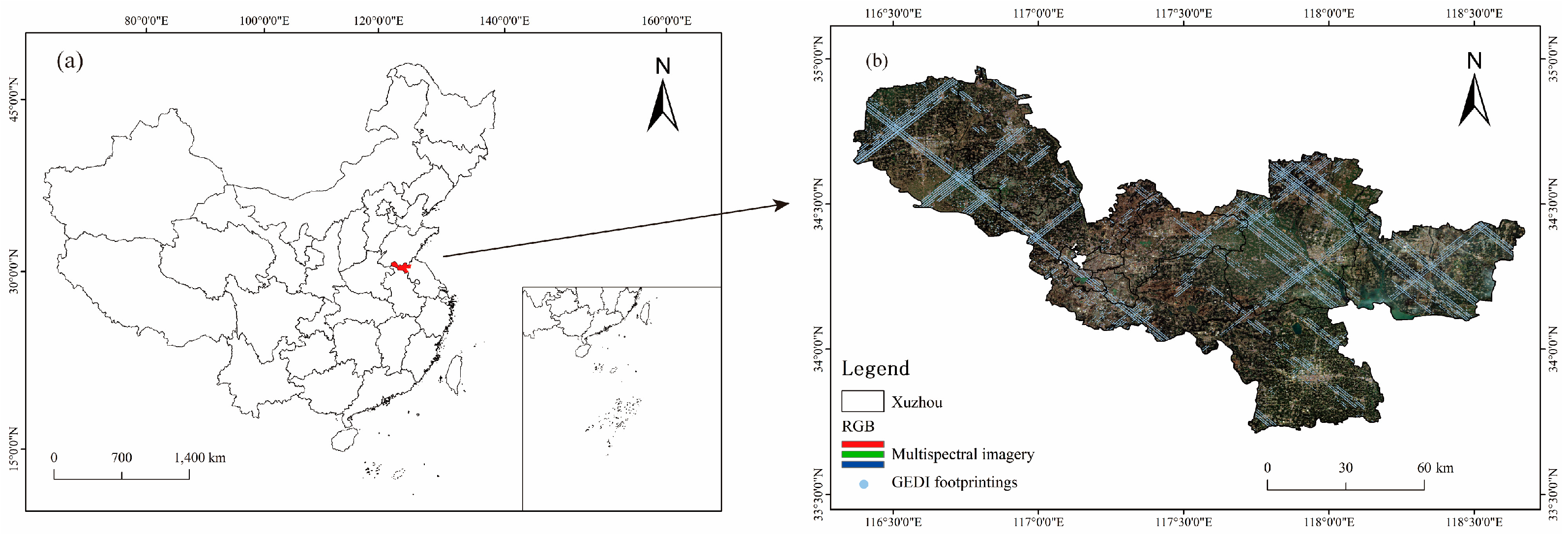
Figure 1. (a) Map of China’s administrative divisions; (b) Xuzhou administrative district, multispectral image and GEDI footprints distribution.
Remotesensing 16 01229 g001
Figure 2. Pictures of field measurements. (a) UAV mapping of forests; (b) tree DBH measurements; (c) shorter vegetation height measurements; (d) laboratory measurement of AGB.
Remotesensing 16 01229 g002
Figure 3. The flowchart of estimating the canopy height and AGB of vegetation using GEDI and optical images.
Remotesensing 16 01229 g003
Figure 4. GEDI waveform. The horizontal coordinate (unit: meter) represents the elevation corresponding to the waveform, and the vertical coordinate represents the normalized voltage value of the waveform after normalization.
Remotesensing 16 01229 g004
Figure 5. (a) Five types of land cover in Xuzhou and field measurement points; (bd) field photos illustrating three typical vegetated areas, (b) the shorter vegetation region; (c) the coniferous forest; and (d) the broadleaf forest.
Remotesensing 16 01229 g005
Figure 6. Distribution of spatially continuous canopy height using GEDI laser points and optical images inversion in four seasonal periods. (a) January–March, (b) April–June, (c) July–September, and (d) October–December.
Remotesensing 16 01229 g006
Figure 7. Distribution of spatially continuous AGB using GEDI laser points and optical images inversion in four seasonal periods. (a) January–March, (b) April–June, (c) July–September, and (d) October–December.
Remotesensing 16 01229 g007
Figure 8. (a) Scatter plot between the canopy height modeled by UAV imagery and the prediction canopy height estimated by optical images; (b) Scatter plot between the canopy height extracted by GEDI and the predicted canopy height estimated by GEDI joint optical images.
Remotesensing 16 01229 g008
Figure 9. Distribution of spatially continuous vegetation canopy height only using optical image inversion. (a) January–March, (b) April–June, (c) July–September, and (d) October–December.
Remotesensing 16 01229 g009
Figure 10. The difference obtained by the canopy height derived from GEDI joint optical images inversion minus the canopy height derived from only optical images inversion in (a) January–March, (b) April–June, (c) July–September, and (d) October–December.
Remotesensing 16 01229 g010
Figure 11. Comparison of four fitting functions for the relationship between max canopy height and measured AGB. (a) cubic function; (b) power function; (c) exponential function; (d) quadratic function.
Remotesensing 16 01229 g011
Figure 12. Comparison of between the measured AGB and the predictions of AGB. (a) Predictions of AGB are obtained by joint inversion of GEDI observations and optical images. (b) Predictions of AGB are obtained by only optical images.
Remotesensing 16 01229 g012
Figure 13. The difference obtained by the AGB derived from GEDI joint optical images inversion minus the AGB derived from only optical images inversion in (a) January–March, (b) April–June, (c) July–September, and (d) October–December.
Remotesensing 16 01229 g013
Figure 14. The importance of feature parameters in the Xuzhou region. The prefix of “L” represents Landsat-8, and the prefix of “S” represents Sentinel-2.
Remotesensing 16 01229 g014
Figure 15. Distribution ratio of AGB from different urban green space types in Xuzhou using GEDI joint optical images. (a) Distribution ratio of AGB from shorter vegetation; (b) Distribution ratio of AGB from broadleaf Forest; (c) Distribution ratio of AGB from coniferous Forest.
Remotesensing 16 01229 g015
Figure 16. Distribution of forest resources in Xuzhou.
Remotesensing 16 01229 g016
Figure 17. The AGB difference between October–December and April–June.
Remotesensing 16 01229 g017
Table 1. Image information.
ImageCountTimeResolutionUse Bands
7March 202130 mCoastal; blue; green; red; NIR; SWIR1; SWIR2
2April 2021
3June 2021
Landsat-84August 2021
2October 2021
4November 2021
4December 2021
5January 2021Prioritize the use of 10 m resolution images, followed by 20 m resolution imagesCoastal; blue; green; red; VRE1; VRE2; VRE3; NIR; Narrow NIR; SWIR1; SWIR2
1February 2021
8March 2021
1April 2021
Sentinel-29May 2021
2June 2021
3July 2021
6September 2021
5November 2021
19December 2021
Table 2. Feature parameters of the vegetated area used in this study.
TypeParametersDescription & EquationReference
Vegetation indicesNDVI(NIR − Red)/(NIR + Red)[50]
GNDVI(NIR − Green)/(NIR + Green)[51]
EVI2.5 × (NIR − Red)/(NIR + 6 × Red − 7.5 × Blue + 1)[51]
NBR(NIR − SWIR)/(NIR + SWIR)[52]
RVINIR/Red[51]
DVINIR − Red[53]
ARVI(NIR − 2 × Red + Blue)/(NIR + 2 × Red − Blue)[51]
Spectral bandsBlueBlue band/
GreenGreen band/
RedRed band/
NIRNIR band/
SWIRSWIR band/
CoastalCoastal band/
VREVegetation red edge band/
Texture feature (gray level co-occurrence matrix window size: 7 × 7 pixels; gray level: 64; moving step length: 1; direction: 45°)Mean i j = 0 N 1 i P i j [54]
Variance i j = 0 N 1 P i j ( i M e a n ) 2 [54]
Homogeneity i j = 0 N 1 P i j P i j 1 + ( i j ) 2 [54]
Dissimilarity i j = 0 N 1 P i j | i j | [54]
Entropy i j = 0 N 1 P i j ( ln P i j ) [54]
Second moment i j = 0 N 1 P i j 2 [54]
Correlation i j = 0 N 1 P i j ( i M e a n ) ( j M e a n ) V a r i a n c e i V a r i a n c e j [54]
Contrast i j = 0 N 1 i P i j ( i j ) 2 [54]
TopographySlopeSlope in degrees/
ElevationElevation above sea level in meters/
Pij represents the probability of each pixel pair (i, j) value and i, j are the gray tones in the windows, which are also the coordinates of the co-occurrence matrix space; N represents the number of distinct grey levels in the quantized image, which has a gray value range of the original image [54].
Table 3. Allometric growth equation for calculating quadrat AGB.
Tree/Shrub SpeciesAGB Model (Mg)Reference
Platycladus orientalis (L.) Franco W = 0.0573 ( D 2 H ) 0.8657 + 0.0043 ( D 2 H ) 1.1085 + 0.0038 ( D 2 H ) 1.3085 [56]
Populus L. W = 0.006 ( D 2 H ) 1.098 + 0.001 ( D 2 H ) 1.157 + 0.012 ( D 2 H ) 0.685 [57]
Cinnamomum camphora (L.) Presl. W = 0.0914 ( D 2 H ) 0.7755 + 0.0099 ( D 2 H ) 1.0256 + 0.0011 ( D 2 H ) 1.1713 [58]
Ginkgo biloba L. W = E X P ( 3.84 + 0.95 l n ( D 2 H ) ) + E X P ( 9.38 + 1.46 l n ( D 2 H ) + E X P ( 6.95 + 1.03 l n ( D 2 H ) ) [59]
Pinoideae Pilger W = E X P ( 2.8319 + 0.8379 l n ( D 2 H ) ) + E X P ( 3.9021 + 0.8822 l n ( D 2 H ) ) + E X P ( 4.0174 + 0.7659 l n ( D 2 H ) ) [60]
Ligustrum lucidum Ait. W = 0.03939 ( D 2 H ) 0.95679 + 0.03357 ( D 2 H ) 0.77809 + 0.11613 ( D 2 H ) 0.45871 [61]
Koelreuteria paniculata Laxm. W = 0.08259 ( D 2 H ) 0.80831 + 0.0053 ( D 2 H ) 1.29104 + 0.01286 ( D 2 H ) 0.69408 [61]
Firmiana platanifolia W = 0.021158 D 2.43244 + 0.057869 D 2.06599 + 0.060045 D 1.54688 [62]
Metasequoia glyptostroboides W = 0.656 + 0.028 ( D 2 H ) 1.258 + 0.007 ( D 2 H ) 0.004 + 0.001 ( D 2 H ) [63]
Other hard broadlesf trees W = 0.07112 ( D 2 H ) 0.910358078 [63]
Other soft broadlesf trees W = 0.012541 ( D 2 H ) 1.144 + 0.00478 ( D 2 H ) 1.006 + 0.04718 ( D 2 H ) 0.769 [63]
Other broadlesf trees W = 0.0452 ( D 2 H ) 0.8741 + 0.0201 ( D 2 H ) 0.8389 + 0.0101 ( D 2 H ) 0.7801 [58]
Other coniferous trees W = 0.0179 ( D 2 H ) 1.089 + 0.0131 ( D 2 H ) 0.8571 + 0.0051 ( D 2 H ) 0.9291 [58]
Photinia serrulata W = 0.805 ( D 2 H ) 1.051 [64]
Hibiscus syriacus W = 206.627 V c 1.589 [64]
Tree-like shrub W = 0.274 D 2.454 [64]
Other shrubs W = 157.759 V c 0.881 [64]
Grass W = 0.63 /
D represents DBH; H represents canopy height; W refers to AGB. V C is the volume of the plant crown (calculated as V C = π C 1 × C 2 × H ( C 1 for north-south crown diameter, C 2 for east-west crown diameter)).
Table 4. Distribution of AGB for different vegetated areas using GEDI joint optical images.
Shorter VegetationBroadleaf ForestConiferous Forest
Total AGB (Mg)25,342,735.525,866,387.54904,178.41
Area (ha)754,389168,76819,404
Average AGB (Mg/ha)33.6034.7646.60
Table 5. Distribution of average AGB in different seasons using GEDI joint optical images.
January–MarchApril–JuneJuly–SeptemberOctober–December
Shorter vegetation (Mg/ha)34.5633.5931.0159.70
Broadleaf forest (Mg/ha)40.9834.7629.4857.42
Coniferous forest (Mg/ha)39.4446.6032.0753.74
Average AGB (Mg/ha)36.0434.2930.9559.55
Disclaimer/Publisher’s Note: The statements, opinions and data contained in all publications are solely those of the individual author(s) and contributor(s) and not of MDPI and/or the editor(s). MDPI and/or the editor(s) disclaim responsibility for any injury to people or property resulting from any ideas, methods, instructions or products referred to in the content.