Abstract
The accurate estimation of forest above-ground biomass (AGB) is vital for monitoring changes in forest carbon sinks. However, the spatial heterogeneity of AGB, coupled with inherent uncertainties, poses challenges in acquiring high-quality AGBs. This study introduced a bias-corrected ensemble machine learning (ML) algorithm for AGB downscaling that integrated a ML for AGB mapping with another for residual mapping. The accuracies of six bias-corrected ensemble ML algorithms were evaluated at resolutions of 0.05°, 0.025°, and 0.01°. Moreover, a step-by-step downscaling (SBSD) method was introduced, utilizing bias-corrected ensemble ML algorithms to downscale AGB from 0.1° to 0.05°, 0.025°, and 0.01° resolutions and was compared with the direct downscaling (DD) at three scales. A comparative analysis was conducted in the Daxing’anling Mountains and Xiaoxing’anling Mountains. AGB and corresponding uncertainty maps at three scales were generated using SBSD. The results showed that the efficacy of the XGBoost-based AGB model combined with the random forest-based residual correction model was superior. Spatial patterns in AGB maps generated by SBSD and DD were found to be similar. Notably, SBSD yielded enhanced accuracy in the Daxing’anling Mountains with complex topography, while both performed comparably in the Xiaoxing’anling Mountains with milder topography, highlighting SBSD’s advantages in high heterogeneity areas.
1. Introduction
The accurate estimation of above-ground biomass (AGB) in forests is essential for addressing climate change, planning forest management, and promoting sustainable development [1,2,3]. Remote sensing techniques have been extensively used for AGB estimation [4]. With the aid of machine learning (ML) algorithms, many AGB products are generated using data from multiple satellites at local or global scales [5]. These published studies predominantly employed upscaling methods, which first compiled field biomass and subsequently utilized satellite data for comprehensive wall-to-wall mapping. However, generating high-resolution AGB maps through upscaling methods necessitates a substantial number of training samples from field data, posing challenges in data acquisition. Additionally, the spatial resolution of the resulting AGB map is constrained by the size of the study plot. Spatial downscaling techniques offer a viable solution to these challenges. In contrast to upscaling methods, downscaling approaches do not demand an extensive number of training samples from field data [6,7]. Furthermore, they mitigate spatial discrepancies between field measurement and satellite data.
Spatial downscaling techniques have been widely used in various fields such as the retrieval of high-resolution soil moisture and climate data [8,9]. Although many methods have been proposed for downscaling such as statistical downscaling and super-resolution, published studies mainly employed the statistical downscaling method owing to its low computational complexity and high model interpretability [10,11]. The statistical downscaling method is implemented by initially establishing statistical models between coarse-resolution target variables and predictors [12]. Subsequently, downscaled maps were generated using the established model and finer-resolution predictors [13]. Until now, there have been few studies dedicated to downscaling forest AGB. Wang and Sun [14] utilized multi-scale geographically weighted regression (MGWR) to downscale AGB from 30 m to 15 m. However, the statistical downscaling method operates under the assumption that a model developed at a coarser resolution can be applied to finer resolutions, a premise that may deviate from reality. As the scale difference increases, the validity of this assumption will diminish, particularly in complex regions characterized by high heterogeneity [15]. To mitigate the impacts of the assumption that estimation models are scale invariant, we introduced the stepwise downscaling method. This approach involves defining multiple intermediate resolutions between the initial resolution and the target resolution. For each intermediate resolution and the final target resolution, spatial downscaling models are employed.
An additional critical aspect of spatial downscaling pertains to the disaggregation of residuals at coarser resolutions, which cannot be explained by models, into finer resolutions. In many studies, all finer pixels within each coarser-resolution pixel are assigned a constant value equal to the residual of the corresponding coarser-resolution pixel. However, this approach may result in to the manifestation of the ‘boxy artifact,’ which indicates that the low-resolution grid is still apparent in the finer resolution disaggregated images [16]. In addition, the spatial variability present at higher resolutions due to variations in AGB has not been taken into account by constant residuals derived at lower resolutions. To address this issue, some studies employed spline tension interpolation [17] or the artificial neural network model [18] to generate a residual map. In this context, we drew inspiration from bias-corrected ML algorithms [19] and examined the efficacy of ensemble ML algorithms in modelling residuals. Liu and Sun [20] utilized multivariate linear stepwise regression and power function methods to downscale AGB from 1 km to 30 m resolution, indicating that the nonlinear regression method is more adept at capturing the nonlinear relationship between AGB and auxiliary variables. ML algorithms which have been demonstrated to perform well in nonlinear modeling and AGB estimation [21] were incorporated for downscaling in this study. Our investigation focused on assessing the performance of ML for AGB and residual mapping, along with identifying optimal combinations for AGB downscaling—serving as one of the primary objectives of this study.
To summarize, the objective of this study is to formulate an optimal SBSD method based on ML algorithms. The specific research contributions included: (1) the development of dual MLs for downscaling, with one ML dedicated to AGB mapping and another to residual mapping; (2) the comparison of various ML combinations to determine the optimal MLs for AGB downscaling; (3) the implementation of the SBSD method to mitigate the impacts of the scale-invariant hypothesis while generating multi-scale forest AGB maps; and (4) the comparison of the SBSD method with the traditional direct downscaling (DD) method to assess the efficacy of the SBSD method in contrast to the traditional DD technique.
2. Data and Methods
2.1. Study Area
Northeastern China is an important timber production base of the country, contributing to approximately 46% of the total forest biomass in China [22] (Figure 1). Geographically, it spans from longitude 115°32′ to 135°09′E and latitude 38°42′ to 53°35′N, encompassing the provinces of Heilongjiang, Jilin, and Liaoning, as well as the eastern part of the Inner Mongolia Autonomous Region. The study region belongs to a temperate continental monsoon climate, with the mean precipitation of 250–1100 mm and temperature of −4–11.5 °C [23].
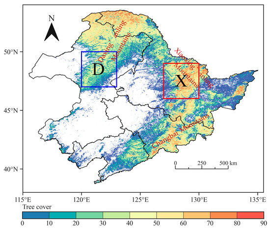
Figure 1.
Study area. Red rectangular box labeled X represents a section of Xiaoxing’anling Mountains. Blue rectangular box labeled D represents a section of Daxing’anling Mountains. Background map shows spatial distribution of tree cover in study area.
The diverse forest ecosystems within the region include warm temperate deciduous broadleaf forests with Korean pine (Pinus koraiensis Sieb. Et Zucc.) as the representative species, temperate coniferous and broadleaf mixed forests with Dahurian larch (Larix gmelinii Rupr.) andWhite Brich (Betula platyphylla Suk.) as the dominant species, and boreal forests with Mongolian pine (Pinus sylvestris var. mongolica Litv.) as the dominant species. These ecosystems are predominantly distributed across three distinct forest regions: the Daxing’anling Mountains, Xiaoxing’anling Mountains, and Changbai Mountains, each covering forest land areas of 15.0, 6.0, and 13.6 million hectares, respectively [24].
2.2. Coarse-Resolution Forest AGB Data
Global AGB maps for the years 2000, 2008, 2010, and 2017, at a resolution of 0.1°, were obtained from https://doi.org/10.6084/m9.figshare.18393689.v1, accessed on 12 June 2023 [25]. The accuracy of the AGB maps closely matched the plot AGB values from the National Forest Inventory in terms of the mean difference and root mean squared difference [26]. Additionally, they also provided baseline AGB values [27]. We used the global AGB map for the year 2010 as the base map for forest AGB downscaling. The base forest AGB map is a bias-corrected AGB map, which originated from a synthesis of spaceborne synthetic aperture radar (SAR), LiDAR, and optical remote sensing data [28]. The uncertainty associated with the original map was assessed using field AGB, and Random Forest (RF) was employed to model the bias. The bias was subsequently used to correct the generated AGB map from Santoro, Cartus [28]. The coarse-resolution AGB map exhibited values ranging from 0.00 to 136.25 Mg/ha, with an average AGB of 20.24 Mg/ha.
2.3. Remote Sensing Data
In accordance with findings from prior research, forest AGB was correlated with various remote sensing parameters, including Nadir bidirectional reflectance distribution function adjusted reflectance (NBAR), net primary productivity (NPP), vegetation continuous fields (VCF), and land surface temperature (LST) [29,30]. In this study, features were extracted from the Moderate Resolution Imaging Spectroradiometer (MODIS) NBAR product at a resolution of 500 m (MCD43A4) [31], annual NPP (MOD17A3HGF) at 500 m resolution [32], the VCF product (MOD44B) at 250 m resolution [33], and LST data (MOD11A2) at 1 km resolution [34] for the year 2010, serving as predictors of forest AGB.
Additionally, we computed the enhanced vegetation index (EVI) and normalized difference infrared index for Band 6 (NDIIB6) from MODIS NBAR data, both considered predictors of forest AGB [35,36].
To mitigate the impact of clouds on LST quality, cloud-affected pixels were excluded based on ‘QC’ flags [37]. To incorporate temporal information from MODIS data [38], percentiles (10th, 25th, 50th, 75th, and 90th) of reflectance, EVI, NDIIB6, and LST were included in the downscaling of forest AGB.
Considering their established correlations with forest AGB [30], the forest canopy height [39], climatological predictors, and topographic predictors were also integrated. Monthly precipitation and temperature data at 0.0083333° (~1km) resolution were obtained from the National Earth System Science Data Center, National Science and Technology Infrastructure of China (http://www.geodata.cn, accessed on 18 July 2023) [40]. Annual mean temperature and annual cumulative precipitation data for the year 2010 were calculated. Elevation and slope data were obtained from the Global Multi-Resolution Terrain Elevation Data 2010 (GMTED2010) product at 7.5 arcsec (~250 m) resolution [41].
The detailed description of these predictor variables is shown in Table 1.

Table 1.
Lists of predictor variables used in study.
The tree cover map, provided by Hansen and Potapov [42] at 0.0025° resolution and obtained from the Global Forest Watch platform (http://www.globalforestwatch.org/, accessed on 12 August 2023), was aggregated to the 0.01° resolution. Pixels with tree cover less than 10% at the 0.01° resolution were defined as non-forest and excluded from the analysis.
2.4. Methods
In this section, we describe the proposed algorithm for AGB estimation and two downscaling methods (Figure 2).
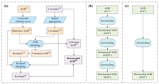
Figure 2.
(a) Flowchart detailing downscaling process for AGB; (b) flowchart of SBSD method; (c) flowchart depicting DD approach.
2.4.1. Bias-Corrected Ensemble ML Algorithms for AGB Mapping
Figure 2a illustrates the flowchart depicting the spatial downscaling process for AGB estimates. The key steps were as follows:
- (1)
- Predictor aggregation and coarse-resolution modeling in (3):
Predictors were aggregated to coarser resolution (e.g., 0.025°, 0.05°, and 0.1° in this study) through averaging. ML algorithms were applied to model AGB at coarse resolutions. The AGB model describes the relationship between the predictor variables and the target AGB at the coarse scale.
where represents the AGB model at the coarse scale, denotes the coarse-scale covariates, and signifies the reference AGB value at the coarse scale.
- (2)
- Estimation of forest AGB at coarse resolutions in (4) and (5):
The trained model was employed to estimate forest AGB at coarse resolutions. Residuals, representing the unexplained portion by ML models, were derived by calculating the difference between reference AGB and estimated AGB based on ML models.
where represents the estimated AGB value at the coarse scale and represents the AGB residual value at the coarse scale.
- (3)
- Residual modeling based on ML algorithms in (6):
The inputs of residual modeling included predictors of AGB and forest AGB at coarse resolutions [19].
where is the residual model at the coarse scale.
- (4)
- Downscaling to finer resolutions in (7)–(9):
Under the assumption of scale invariance, forest AGB at finer resolutions was estimated based on the AGB model developed in step (2) and AGB residuals were from the AGB residual model developed step (3). The derived high-resolution AGB should be corrected using the AGB residual. The downscaled AGB was calculated as the sum of estimated AGB and AGB residuals at a finer resolution.
where is indicative of the estimated AGB value at the fine scale, signifies the fine-scale residual value, and represents the downscaled AGB at the fine scale.
As shown in step (4), the proposed method utilized the high-resolution residuals derived from the ML algorithms to correct the high-resolution AGB. The downscaled AGB was not affected by “box artifacts”, since the approach does not assume that the contribution to the residuals by the fine-resolution pixels constituting the coarse-resolution pixels is constant. Meanwhile, the residual model, by incorporating multiple predictor variables such as AGB, topography, etc., could capture complex nonlinear statistical relationships and enhance certain spatial details.
In this study, ensemble ML algorithms RF and XGBoost were employed for AGB and AGB residual modeling. RF, a tree-based ensemble algorithm utilizing subsamples and a random subset of features [43], exhibits excellent performance in estimating AGB [44]. XGBoost, a boosting algorithm that transforms weak learners into strong learners by increasing the weights of samples with errors in multiple iterations, has proven effective for AGB retrieval [44,45]. The multilayer perceptron (MLP) has been recognized as a reliable model for forest AGB estimation [46]. To identify optimal models for AGB downscaling, we compared the performance of RF, XGBoost, and MLP for AGB modeling, as well as the performances of RF and XGBoost for residual modeling.
To reduce the impacts of spatial averaging effect on downscaled results, AGB correction based on tree cover was implemented. Specifically, tree cover data from Hansen and Potapov [42] were aggregated to coarse resolution, and AGB was divided by tree cover. The tree cover-corrected forest AGB data, serving as the reference AGB, were utilized to establish the AGB model and validate the accuracy of the estimated AGB.
2.4.2. Proposed Step-by-Step Spatial Downscaling Method
When there is a large difference in spatial resolution between fine-resolution predictor variables and coarse-resolution AGB, the assumption of scale invariance is difficult to satisfy. A significant limitation of the downscaling method, particularly when employing ML algorithms, lies in the presumption that the model developed in step (1) remains applicable across diverse spatial scales. The training data, utilized to develop the model at a coarse scale, essentially averages out the spatial variability present. Consequently, as the gap in spatial resolutions between the fine-scale predictor variables and the coarse-scale AGB widens, the downscaled AGB does not accurately characterize the spatial distribution of the AGB, especially in areas with high spatial heterogeneity. Given that ML algorithms tend to struggle with predicting datasets that fall outside the range of training data, coarse-resolution models are unlikely to effectively incorporate the finer spatial details.
In order to mitigate the potential impact of the assumption that the AGB model is scale-invariant, we introduced the SBSD method (Figure 2b). This method substantially enhanced the spatial resolution of AGB with high accuracy via a series of small-scale spatial resolution downscaling steps. Throughout the operation of the SBSD method, each downscaling phase integrated finer predictor variables into the models. Consequently, this methodology enhanced the accuracy in capturing the relationship between AGB and predictor variables.
In this research, the SBSD method involved downscaling the AGB from the original 0.1° resolution to 0.05°, then further to 0.025°, and ultimately to 0.01°, employing the proposed bias-corrected ensemble ML algorithms. The SBSD method was systematically evaluated against the conventional DD approach, wherein forest AGB is directly downscaled from 0.1° to the target resolution of 0.01° (Figure 2c).
2.5. Accuracy Assessment
In this study, we employed the 10-fold cross-validation (CV) method to assess the performance of the downscaling models. The evaluation metrics utilized included the coefficient of determination (R2), mean absolute error (MAE), bias, and root mean square error (RMSE).
The metrics are defined as follows:
where represents the total number of test samples, is the mean of the reference AGB, denotes the reference AGB, and represents the predicted AGB.
3. Results
3.1. Performances of Bias-Corrected ML Downscaling Algorithms for AGB Mapping
Table 2 presents the average performance across 10 runs at 0.1° resolution for each of the 6 downscaled models. The findings indicated a consistent superior of RF-based residual models over their XGBoost-based counterparts in terms of RMSE and MAE. Notably, the XGBoost-RF downscaling model, wherein XGBoost is employed for AGB estimation and RF for residual modeling, achieved the highest accuracy in AGB estimates at 0.1° resolution. Conversely, the MLP-XGBoost downscaling model exhibited the lowest accuracy. These results at 0.1° resolution were also established at resolutions of 0.05° and 0.025° when employing the SBSD method, underscoring the stability of model performances.
Table 2.
Average performance metrics for 10 runs of 6 downscaling models at 0.1° resolution.
3.2. Downscaled Forest AGB Maps Using SBSD and DD
The ten developed XGBoost-RF models were employed to generate forest AGB maps. The final downscaled results, shown in Figure 3, were derived as the mean values of the ten AGB maps, with the standard deviations of the ten generated results utilized to indicate the uncertainty with the AGB maps (Figure 4). The SBSD method produced multi-scale AGB maps with spatial resolutions of 0.05°, 0.025°, and 0.01°.
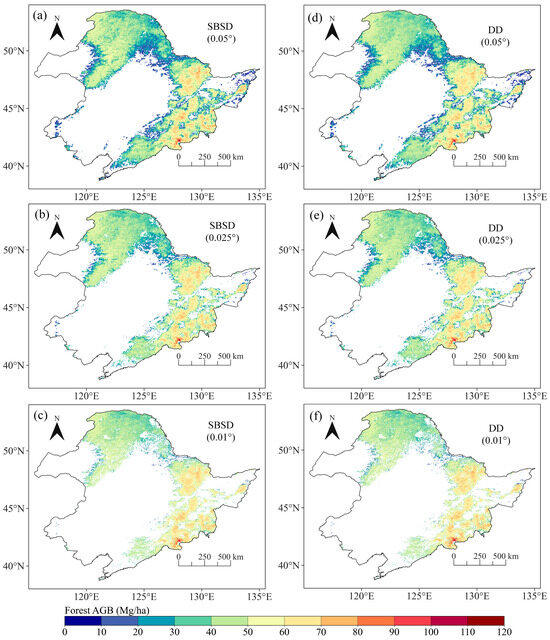
Figure 3.
Comparative analysis of multi-scale AGB maps derived by SBSD method and corresponding aggregated AGB maps obtained through DD method. (a–c) Downscaled AGB using SBSD method at 0.05°, 0.025°, and 0.01° resolutions; (d–f) aggregated AGB maps.
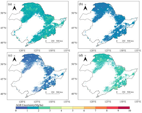
Figure 4.
(a–c) Spatial pattern of AGB uncertainties derived by SBSD method at 0.05°, 0.025°, and 0.01° resolutions. (d) Spatial pattern of AGB uncertainty obtained through DD method at 0.01° resolution.
In order to compare the downscaled AGB results using SBSD and DD, we aggregated the DD downscaled AGB at 0.01° resolution to 0.025° and 0.05° by averaging. The comparison results suggested a consistent spatial distribution of AGB maps generated using SBSD with those resulting from DD. Higher AGB values were predominantly observed in the Changbai Mountains and the Xiaoxing’anling Mountains, characterized by dense forest cover (Figure 1), aligning with findings from previous studies [23,47]. Figure 5 illustrates the AGB map in the Daxing’anling Mountains, which is one of the areas with complex topography in the study area. The downscaled AGB maps using SBSD and DD methods in Figure 5 showed more spatial details than the coarse-scale reference AGB maps. In addition, at three scales, the AGB maps using the SBSD method were more consistent with the details observed in the reference AGB map than the conventional DD method. As shown in Figure 6a–c, the AGB distributions using DD and SBSD exhibited similar statistical patterns across the three scales. Overall, AGB values at the 0.01° scale were higher than those at 0.025° and 0.05° scales.
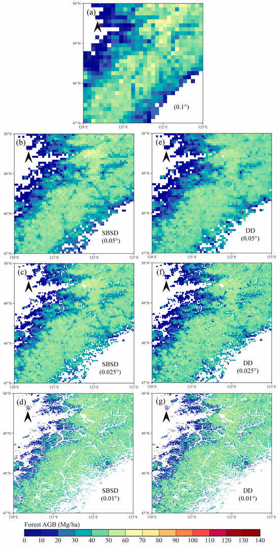
Figure 5.
Magnified perspective of area labeled D in Figure 3. (a) Reference AGB at 0.1° resolution; (b–d) downscaled AGB using SBSD method at 0.05°, 0.025°, and 0.01° resolutions; (e–g) aggregated AGB maps.
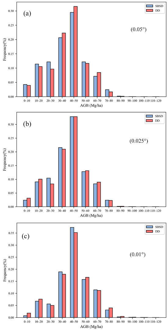
Figure 6.
(a–c) Histogram of downscaled forest AGB using SBSD and DD methods at 0.05°, 0.025°, and 0.01° resolutions.
To examine pixel-level disparities between SBSD results and DD results, AGB difference maps were obtained at three resolutions (Figure 7a–c). Pixels with difference values falling within the range of −5 to 5 Mg/ha were categorized as “no change”. The majority of forest AGB difference values ranged from −10 to 10 Mg/ha (Figure 7d–f). Approximately 52%, 42%, and 38% of the pixels exhibited a difference value between −10 to −5 Mg/ha at 0.05°, 0.025°, and 0.01° resolutions, respectively. Additionally, around 27%, 37%, and 60% of the pixels have a difference within the range of 5–10 Mg/ha at 0.05°, 0.025°, and 0.01° resolutions. These findings suggested that at 0.05° and 0.025° scales, in most forest areas, AGB values obtained through DD were generally higher than those obtained through SBSD. Conversely, at the 0.01° scale, AGB values obtained through DD were generally lower than those obtained through SBSD.
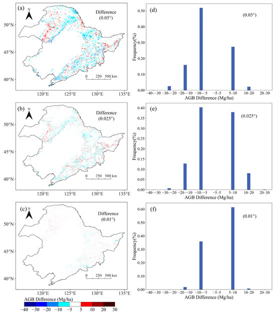
Figure 7.
(a–c) Difference maps between AGB obtained through SBSD and corresponding aggregated AGB maps by DD method at resolutions of 0.05°, 0.025°, and 0.01°; (d–f) pixel frequency histograms associated with AGB difference.
Additionally, notable differences in AGB between DD and SBSD were observed across three resolutions, particularly in regions characterized by high and low elevations. This emphasizes the significance of complex mountainous terrain in the downscaling of AGB, as suggested by Wang and Sun [14]. Subsequently, a detailed analysis of AGB difference maps was conducted in the high-elevation areas of the Daxing’anling Mountains (Figure 8) and the low-elevation areas of the Xiaoxing’anling Mountains (Figure 9). As shown in Figure 8, across all three scales, the percentage of positive difference values of difference was notably higher in high-elevation areas, indicating that the AGB values derived through SBSD were higher than those obtained through DD in complex mountainous environments. Furthermore, with an increase in spatial resolution, the percentage of positive values exhibited an upward trend, highlighting the advantage of SBSD in more complex areas. As shown in Figure 10, the standard deviations of AGB difference values were the highest within the elevation range of 800–1000 m, followed by the range of 1200–1500 m. This pattern may be attributed to the fact that the elevation range of 800–1000 m primarily encompasses transitional zones between higher and lower elevations. In essence, both in transitional zones and high-elevation areas, the standard deviations of AGB differences were higher, indicating greater variation in the AGB difference values. In areas with steeper slopes, the standard deviations of the AGB difference values were smaller, indicating less variation in AGB differences. The relatively small AGB differences in the central part of the region may be attributed to the influence of slope. In flatter terrain, specifically in spatially homogeneous areas, the percentage of negative difference values was higher at the 0.05° scale. Although this trend persisted at the 0.025° scale, at the 0.01° scale the percentage of negative difference values was close to the percentage of positive difference values (Figure 9). This indicated a diminishing advantage of SBSD in areas characterized by low heterogeneity.
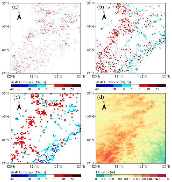
Figure 8.
(a–c) AGB difference maps in high-elevation area of Daxing’anling Mountains at 0.01°, 0.025°, and 0.05° resolutions; (d) corresponding elevation map.
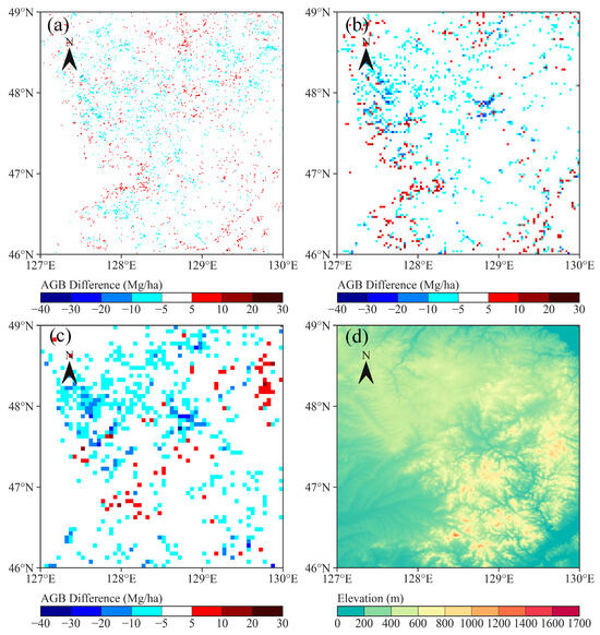
Figure 9.
(a–c) AGB difference maps in low-elevation area of Xiaoxing’anling Mountains at 0.01°, 0.025°, and 0.05° resolutions; (d) corresponding elevation map.
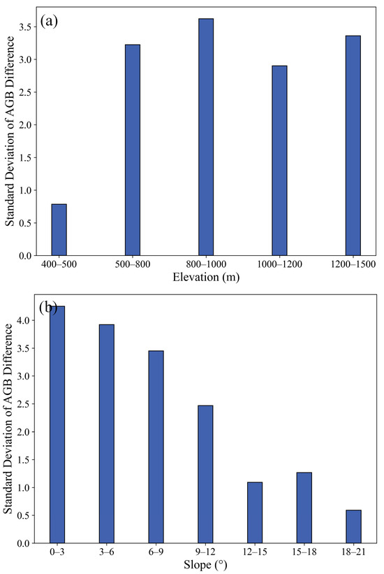
Figure 10.
High-elevation area of Daxing’anling Mountains. (a) Standard deviation of AGB difference per elevation class; (b) standard deviation of AGB difference per slope class.
We conducted a comparative analysis of carbon stocks between the DD and SBSD methods. The total forest biomass in the northeast region for the year 2010 was calculated by summing the AGB of all forest pixels. The corresponding carbon stocks were computed by applying a standardized coefficient of 0.5 (Table 3) [48]. At the initial resolution of 0.1°, the carbon stock was estimated at 1.438 Pg C. From 0.1° to 0.05° scale, the carbon difference was 0.036 Pg C and 0.061 Pg C for DD and SBSD methods, respectively. From 0.05° to 0.025° scale, the carbon difference was 0.072 Pg C and 0.049 Pg C for DD and SBSD methods, respectively. From 0.025° to 0.01° scale, carbon difference was 0.184 Pg C and 0.180 Pg C for DD and SBSD methods, respectively. From 0.1° to 0.05° scale, the percentages of the carbon difference were 2.5% and 4.2% for DD and SBSD methods, respectively. From 0.05° to 0.025° scale, the percentages of the carbon difference were 5.1% and 3.6% for DD and SBSD methods, respectively. From 0.025° to 0.01° scale, the percentages of the carbon difference were 13.8% and 13.6% for DD and SBSD methods, respectively. When the spatial resolution went from 0.1° to 0.01°, the percentage of carbon differences for DD and SBSD methods all showed an overall increase. This indicated that when the spatial resolution increased, the variation of carbon stock also increased. Simultaneously, the forest area was 70.82, 64.97, and 51.4 million ha at 0.05°, 0.025°, and 0.01° scales, respectively. The different forest areas at three scales were attributed to the effect of mixed forest pixels. At low spatial resolutions, there were a large number of mixed forest pixels. With the increase in spatial resolution, non-forest pixels that were counted within forest pixels at the coarse resolutions were excluded, resulting in progressively smaller forest areas and corresponding smaller carbon stocks. The SBSD method demonstrated a lower carbon stock difference compared to the DD method.
Table 3.
Corresponding forest carbon storage, forest area, and percentage of difference of downscaled forest AGB using DD and SBSD methods at various resolutions.
4. Discussion
4.1. Uncertainties of AGB Estimates by Using Spatial Downscaling
Methods based on remote sensing data for AGB estimation still have substantial uncertainties [49,50]. Uncertainty analysis is considered a crucial tool to determine factors influencing the performance of downscaled models, enabling model optimization [51]. The sources of downscaled AGB uncertainty at each scale emanates from errors in the input data and downscaled models employed [6,52]. In this study, the 10-fold CV is used to quantify model uncertainty. The uncertainty of input data, including errors in input AGB, can affect the accuracy of the downscaled AGB results, but has not been considered [6]. Previous studies predominantly addressed input data uncertainty through the error propagation method [53,54].
Furthermore, within the SBSD process, errors can propagate from the initial level to the final level, affecting the accuracy of downscaled AGB. In response, we addressed the errors in the input data of the downscaled model at subsequent levels through residual correction applied to the predicted AGB at the previous level and correcting the downscaled AGB at the previous level using tree cover data, contributing to error mitigation in the SBSD framework.
Figure 4 presents the spatial distribution of multi-scale forest AGB uncertainty maps in Northeast China. High uncertainties were observed in the high AGB areas, consistent with results of previous studies [50]. The AGB uncertainty employing SBSD at the 0.05° scale and the AGB uncertainty employing DD at the 0.01° scale demonstrated close similarity due to the fact that the main component of both was the model uncertainty at the 0.1° scale. With the increase in resolution, the AGB uncertainties employing SBSD diminished. This reduction was because the SBSD method involves multiple residual corrections, which effectively reduced the model uncertainty at each resolution.
4.2. Performances of Bias-Corrected ML Downscaling Algorithms
In this study, the bias-corrected ML downscaling algorithm proposed consists of the AGB model and residual model. We explored the performances of six ML combinations in estimating forest AGB. Our results suggested that the four tree-based ML combinations, including XGBoost-RF, XGBoost-XGBoost, RF-XGBoost, and RF-RF algorithms, demonstrated similar accuracies in terms of estimated AGB. In contrast, the prediction accuracies of the MLP-XGBoost and MLP-RF models were lower. This discrepancy can be attributed to the inherent instability and heightened sensitivity of the MLP algorithm to the training dataset, consistent with the results of Zhang et al. [21]. Some published results have also showed bias correction methods based on tree-based ML models outperformed other bias correction methods [55]. He and Chaney [56] found that the performance of a double RF for downscaling precipitation was superior compared to a single RF. Therefore, considering different combinations of ML algorithms can optimize performance when determining the most suitable ML algorithm combination.
4.3. Advantages and Limitations of the Stepwise Spatial Downscaling Method
In general, the SBSD method outperformed the DD method in terms of the accuracy of AGB downscaling. This discrepancy can be attributed to the SBSD method’s incorporation of intermediate resolutions and a great number of downscaling processes compared to the DD method. The scale difference between these processes is smaller in the SBSD approach than in the DD process. Moreover, the SBSD method involves multiple residual correction processes. In the DD process, the substantial scale difference between the initial resolution and the target resolution may lead to information loss, resulting in suboptimal accuracy of the residuals from the residual models. However, the relatively small-scale difference in the SBSD method reduces the impacts of scale invariance assumption, thereby enhancing the accuracy of residual models obtained from each resolution.
In spatially complex regions with high heterogeneity, the SBSD method was more advantageous than the DD method. This phenomenon can be attributed to the greater residual accuracy of the SBSD method in complex regions and the fact that it is more adept at capturing spatial information through multiple residual correction processes. In spatially homogenous regions, the advantage of the SBSD method weakened. This is due to the fact that the impact of the scale invariance assumption was reduced, resulting in the residual accuracy of the DD method was close to that of the SBSD method.
Furthermore, at 0.05° and 0.025° resolutions, the carbon stock of the DD method slightly exceeded that of the SBSD method. However, it remained lower than that valued derived from the TRIPLEX 1.0 model (1.4–1.6 Pg C) [57] and the 1.55 Pg C estimate using GLAS and MODIS Data [58]. At the 0.01° scale, the carbon stock values from both methods approached the value of 1.045 Pg C obtained using the biomass-volume model proposed by Wei and Yu [59]. It is important to note that differences in forest definitions across these studies may introduce uncertainties in forest carbon stock estimates.
It is noteworthy that the downscaling model exhibited a tendency to underestimate high biomass values. This discrepancy may come from the intricate structure of forests and spectral saturation of optical remote sensing images, resulting in estimation errors in high biomass areas. Future improvements could involve Radar and LiDAR data for AGB downscaling algorithms to enhance the accuracy of downscaling models. Additionally, deep learning, including convolutional neural networks, offers innovative avenues to invert downscaling products, presenting opportunities to enhance model performance. Finally, careful consideration of the setting of intermediate resolution sequences in the SBSD method is crucial, as it directly impacts model accuracy. Future research should focus on selecting the most appropriate intermediate resolutions based on different scenarios, ensuring the refinement and optimization of the SBSD methodology.
5. Conclusions
In this study, we introduced bias-corrected ensemble ML algorithms and conducted a comprehensive comparison of six such algorithms at resolutions of 0.05°, 0.025°, and 0.01°. The findings revealed that the XGBoost-RF downscaling model exhibited greater accuracy in predicting AGB prediction at all three scales. Additionally, we proposed the SBSD framework based on bias-corrected ensemble ML algorithms and compared it with the DD method. The results suggested that the SBSD method outperformed the DD method and was more suitable for downscaling studies of AGB in complex terrain regions, while the downscaled AGB results using DD and SBSD were closely aligned in spatially homogeneous regions. Moreover, the SBSD method demonstrated a smaller carbon stock difference compared to the DD method.
Furthermore, we employed the optimal SBSD method to generate forest AGB maps and associated uncertainty maps for 2010 at resolutions of 0.05°, 0.025°, and 0.01°. The methodology proposed in this study is applicable to larger spatial scales, such as China or global regions, and can be readily extended to higher spatial resolutions, representing a potential avenue for future research.
Author Contributions
Y.Z. and J.L. conceived the study; Y.Z. and J.L. performed the data analysis; Y.Z. and J.L. contributed to the writing of the manuscript. All authors have read and agreed to the published version of the manuscript.
Funding
This research received no external funding.
Data Availability Statement
No new data were created or analyzed in this study. Data sharing is not applicable to this article.
Conflicts of Interest
The authors declare no conflicts of interest.
References
- Pan, Y.; Birdsey, R.A.; Phillips, O.L.; Jackson, R.B. The structure, distribution, and biomass of the world’s forests. Annu. Rev. Ecol. Evol. Syst. 2013, 44, 593–622. [Google Scholar] [CrossRef]
- Mitchard, E.T. The tropical forest carbon cycle and climate change. Nature 2018, 559, 527–534. [Google Scholar] [CrossRef]
- Lu, D. The potential and challenge of remote sensing-based biomass estimation. Int. J. Remote Sens. 2006, 27, 1297–1328. [Google Scholar] [CrossRef]
- Zheng, D.; Rademacher, J.; Chen, J.; Crow, T.; Bresee, M.; Le Moine, J.; Ryu, S.-R. Estimating aboveground biomass using Landsat 7 ETM+ data across a managed landscape in northern Wisconsin, USA. Remote Sens. Environ. 2004, 93, 402–411. [Google Scholar] [CrossRef]
- Zhang, Y.; Liang, S.; Yang, L. A Review of Regional and Global Gridded Forest Biomass Datasets. Remote Sens. 2019, 11, 2744. [Google Scholar] [CrossRef]
- Ge, Y.; Jin, Y.; Stein, A.; Chen, Y.; Wang, J.; Wang, J.; Cheng, Q.; Bai, H.; Liu, M.; Atkinson, P.M. Principles and methods of scaling geospatial Earth science data. Earth-Sci. Rev. 2019, 197, 102897. [Google Scholar] [CrossRef]
- Markham, K.; Frazier, A.E.; Singh, K.K.; Madden, M. A review of methods for scaling remotely sensed data for spatial pattern analysis. Landsc. Ecol. 2023, 38, 619–635. [Google Scholar] [CrossRef]
- Hutengs, C.; Vohland, M. Downscaling land surface temperatures at regional scales with random forest regression. Remote Sens. Environ. 2016, 178, 127–141. [Google Scholar] [CrossRef]
- Tian, J.; Deng, X.; Su, H. Intercomparison of two trapezoid-based soil moisture downscaling methods using three scaling factors. Int. J. Digit. Earth 2019, 12, 485–499. [Google Scholar] [CrossRef]
- Li, N.; Wu, H.; Ouyang, X. Localized Downscaling of Urban Land Surface Temperature—A Case Study in Beijing, China. Remote Sens. 2022, 14, 2390. [Google Scholar] [CrossRef]
- Ha, W.; Gowda, P.H.; Howell, T.A. A review of downscaling methods for remote sensing-based irrigation management: Part I. Irrig. Sci. 2013, 31, 831–850. [Google Scholar] [CrossRef]
- Agathangelidis, I.; Cartalis, C. Improving the disaggregation of MODIS land surface temperatures in an urban environment: A statistical downscaling approach using high-resolution emissivity. Int. J. Remote Sens. 2019, 40, 5261–5286. [Google Scholar] [CrossRef]
- Wigley, T.M.L.; Jones, P.D.; Briffa, K.R.; Smith, G. Obtaining sub-grid-scale information from coarse-resolution general circulation model output. J. Geophys. Res. Atmos. 1990, 95, 1943–1953. [Google Scholar] [CrossRef]
- Wang, N.; Sun, M.; Ye, J.; Wang, J.; Liu, Q.; Li, M. Spatial downscaling of forest above-ground biomass distribution patterns based on Landsat 8 OLI images and a multiscale geographically weighted regression algorithm. Forests 2023, 14, 526. [Google Scholar] [CrossRef]
- Li, X.; Zhang, G.; Zhu, S.; Xu, Y. Step-By-Step Downscaling of Land Surface Temperature Considering Urban Spatial Morphological Parameters. Remote Sens. 2022, 14, 3038. [Google Scholar] [CrossRef]
- Agam, N.; Kustas, W.P.; Anderson, M.C.; Li, F.; Neale, C.M. A vegetation index based technique for spatial sharpening of thermal imagery. Remote Sens. Environ. 2007, 107, 545–558. [Google Scholar] [CrossRef]
- Duan, Z.; Bastiaanssen, W.G.M. First results from Version 7 TRMM 3B43 precipitation product in combination with a new downscaling–calibration procedure. Remote Sens. Environ. 2013, 131, 1–13. [Google Scholar] [CrossRef]
- Bindhu, V.M.; Narasimhan, B.; Sudheer, K.P. Development and verification of a non-linear disaggregation method (NL-DisTrad) to downscale MODIS land surface temperature to the spatial scale of Landsat thermal data to estimate evapotranspiration. Remote Sens. Environ. 2013, 135, 118–129. [Google Scholar] [CrossRef]
- Zhang, G.; Lu, Y. Bias-corrected random forests in regression. J. Appl. Stat. 2012, 39, 151–160. [Google Scholar] [CrossRef]
- Liu, Q.; Sun, R. Spatial downscaling of forest biomass based on remote sensing. Acta Ecol. Sin. 2019, 39, 3967–3977. [Google Scholar]
- Zhang, Y.; Ma, J.; Liang, S.; Li, X.; Li, M. An Evaluation of Eight Machine Learning Regression Algorithms for Forest Aboveground Biomass Estimation from Multiple Satellite Data Products. Remote Sens. 2020, 12, 4015. [Google Scholar] [CrossRef]
- Yu, D.; Zhou, L.; Zhou, W.; Ding, H.; Wang, Q.; Wang, Y.; Wu, X.; Dai, L. Forest management in Northeast China: History, problems, and challenges. Environ. Manag. 2011, 48, 1122–1135. [Google Scholar] [CrossRef] [PubMed]
- Tan, K.; Piao, S.; Peng, C.; Fang, J. Satellite-based estimation of biomass carbon stocks for northeast China’s forests between 1982 and 1999. For. Ecol. Manag. 2007, 240, 114–121. [Google Scholar] [CrossRef]
- Zhang, X.; Wang, W.-C.; Fang, X.; Ye, Y.; Zheng, J. Vegetation of Northeast China during the late seventeenth to early twentieth century as revealed by historical documents. Reg. Environ. Chang. 2011, 11, 869–882. [Google Scholar] [CrossRef]
- Araza, A.; de Bruin, S.; Herold, M.; Quegan, S.; Labriere, N.; Rodriguez-Veiga, P.; Avitabile, V.; Santoro, M.; Mitchard, E.T.; Ryan, C.M.; et al. A comprehensive framework for assessing the accuracy and uncertainty of global above-ground biomass maps. Remote Sens. Environ. 2022, 272, 112917. [Google Scholar] [CrossRef]
- McRoberts, R.E.; Tomppo, E.O. Remote sensing support for national forest inventories. Remote Sens. Environ. 2007, 110, 412–419. [Google Scholar] [CrossRef]
- Csillik, O.; Asner, G.P. Near-real time aboveground carbon emissions in Peru. PLoS ONE 2020, 15, e0241418. [Google Scholar] [CrossRef] [PubMed]
- Santoro, M.; Cartus, O.; Carvalhais, N.; Rozendaal, D.M.A.; Avitabile, V.; Araza, A.; de Bruin, S.; Herold, M.; Quegan, S.; Rodríguez-Veiga, P.; et al. The global forest above-ground biomass pool for 2010 estimated from high-resolution satellite observations. Earth Syst. Sci. Data 2021, 13, 3927–3950. [Google Scholar] [CrossRef]
- Zhang, Y.; Liu, J.; Li, W.; Liang, S. A Proposed Ensemble Feature Selection Method for Estimating Forest Aboveground Biomass from Multiple Satellite Data. Remote Sens. 2023, 15, 1096. [Google Scholar] [CrossRef]
- Xu, L.; Saatchi, S.S.; Yang, Y.; Yu, Y.; Pongratz, J.; Bloom, A.A.; Bowman, K.; Worden, J.; Liu, J.; Yin, Y.; et al. Changes in global terrestrial live biomass over the 21st century. Sci. Adv. 2021, 7, eabe9829. [Google Scholar] [CrossRef]
- Schaaf, C.B.; Gao, F.; Strahler, A.H.; Lucht, W.; Li, X.; Tsang, T.; Strugnell, N.C.; Zhang, X.; Jin, Y.; Muller, J.-P.; et al. First operational BRDF, albedo nadir reflectance products from MODIS. Remote Sens. Environ. 2002, 83, 135–148. [Google Scholar] [CrossRef]
- Running, S.; Zhao, M. MODIS/Terra Net Primary Production Gap-Filled Yearly L4 Global 500m SIN Grid V061; NASA EOSDIS Land Processes DAAC: Sioux Falls, SD, USA, 2021.
- DiMiceli, C.; Carroll, M.; Sohlberg, R.; Kim, D.H.; Kelly, M.; Townshend, J.R.G. MOD44B MODIS/Terra Vegetation Continuous Fields Yearly L3 Global 250m SIN Grid V006; NASA EOSDIS Land Processes DAAC: Sioux Falls, SD, USA, 2015; Volume 10.
- Hulley, G.; Hook, S. MODIS/Terra Land Surface Temperature/3-Band Emissivity Daily L3 Global 1km SIN Grid Night V061; NASA EOSDIS Land Process DAAC: Sioux Falls, SD, USA, 2021.
- Huete, A.; Didan, K.; Miura, T.; Rodriguez, E.P.; Gao, X.; Ferreira, L.G. Overview of the radiometric and biophysical performance of the MODIS vegetation indices. Remote Sens. Environ. 2002, 83, 195–213. [Google Scholar] [CrossRef]
- Hunt, E.R., Jr.; Rock, B.N. Detection of changes in leaf water content using near-and middle-infrared reflectances. Remote Sens. Environ. 1989, 30, 43–54. [Google Scholar]
- Xie, F.; Fan, H. Deriving drought indices from MODIS vegetation indices (NDVI/EVI) and Land Surface Temperature (LST): Is data reconstruction necessary? Int. J. Appl. Earth Obs. Geoinf. 2021, 101, 102352. [Google Scholar] [CrossRef]
- Zhang, Y.; Liu, J. Estimating forest aboveground biomass using temporal features extracted from multiple satellite data products and ensemble machine learning algorithm. Geocarto Int. 2022, 38, 2153930. [Google Scholar] [CrossRef]
- Simard, M.; Pinto, N.; Fisher, J.B.; Baccini, A. Mapping forest canopy height globally with spaceborne lidar. J. Geophys. Res. Biogeosciences 2011, 116, 4021. [Google Scholar] [CrossRef]
- Peng, S.; Ding, Y.; Liu, W.; Li, Z. 1 km monthly temperature and precipitation dataset for China from 1901 to 2017. Earth Syst. Sci. Data 2019, 11, 1931–1946. [Google Scholar] [CrossRef]
- Danielson, J.J.; Gesch, D.B. Global Multi-Resolution Terrain Elevation Data 2010 (GMTED2010); US Geological Survey: Reston, VA, USA, 2011.
- Hansen, M.C.; Potapov, P.V.; Moore, R.; Hancher, M.; Turubanova, S.A.; Tyukavina, A.; Thau, D.; Stehman, S.V.; Goetz, S.J.; Loveland, T.R.; et al. High-resolution global maps of 21st-century forest cover change. Science 2013, 342, 850–853. [Google Scholar] [CrossRef] [PubMed]
- Breiman, L. Random forests. Mach. Learn. 2001, 45, 5–32. [Google Scholar] [CrossRef]
- Zhang, Y.; Liu, J.; Shen, W. A Review of Ensemble Learning Algorithms Used in Remote Sensing Applications. Appl. Sci. 2022, 12, 8654. [Google Scholar] [CrossRef]
- Bühlmann, P.; Hothorn, T. Boosting Algorithms: Regularization, Prediction and Model Fitting; Institute Of Mathematical Statistics: Beachwood, OH, USA, 2008. [Google Scholar]
- Englhart, S.; Keuck, V.; Siegert, F. Modeling Aboveground Biomass in Tropical Forests Using Multi-Frequency SAR Data—A Comparison of Methods. IEEE J. Sel. Top. Appl. Earth Obs. Remote Sens. 2012, 5, 298–306. [Google Scholar] [CrossRef]
- Zhang, Y.; Liang, S. Changes in forest biomass and linkage to climate and forest disturbances over Northeastern China. Glob. Chang. Biol. 2014, 20, 2596–2606. [Google Scholar] [CrossRef] [PubMed]
- Myneni, R.B.; Dong, J.; Tucker, C.J.; Kaufmann, R.K.; Kauppi, P.E.; Liski, J.; Zhou, L.; Alexeyev, V.; Hughes, M.K. A large carbon sink in the woody biomass of Northern forests. Proc. Natl. Acad. Sci. USA 2001, 98, 14784–14789. [Google Scholar] [CrossRef] [PubMed]
- Réjou-Méchain, M.; Barbier, N.; Couteron, P.; Ploton, P.; Vincent, G.; Herold, M.; Mermoz, S.; Saatchi, S.; Chave, J.; de Boissieu, F.; et al. Upscaling forest biomass from field to satellite measurements: Sources of errors and ways to reduce them. Surv. Geophys. 2019, 40, 881–911. [Google Scholar] [CrossRef]
- Rodríguez-Veiga, P.; Wheeler, J.; Louis, V.; Tansey, K.; Balzter, H. Quantifying forest biomass carbon stocks from space. Curr. For. Rep. 2017, 3, 1–18. [Google Scholar] [CrossRef]
- Wang, G.; Oyana, T.; Zhang, M.; Adu-Prah, S.; Zeng, S.; Lin, H.; Se, J. Mapping and spatial uncertainty analysis of forest vegetation carbon by combining national forest inventory data and satellite images. For. Ecol. Manag. 2009, 258, 1275–1283. [Google Scholar] [CrossRef]
- Zhang, L.; Yu, G.; Gu, F.; He, H.; Zhang, L.; Han, S. Uncertainty analysis of modeled carbon fluxes for a broad-leaved Korean pine mixed forest using a process-based ecosystem model. J. For. Res. 2012, 17, 268–282. [Google Scholar] [CrossRef]
- Xu, Q.; Man, A.; Fredrickson, M.; Hou, Z.; Pitkänen, J.; Wing, B.; Ramirez, C.; Li, B.; Greenberg, J.A. Quantification of uncertainty in aboveground biomass estimates derived from small-footprint airborne LiDAR. Remote Sens. Environ. 2018, 216, 514–528. [Google Scholar] [CrossRef]
- Rodríguez-Veiga, P.; Saatchi, S.; Tansey, K.; Balzter, H. Magnitude, spatial distribution and uncertainty of forest biomass stocks in Mexico. Remote Sens. Environ. 2016, 183, 265–281. [Google Scholar] [CrossRef]
- Belitz, K.; Stackelberg, P.E. Evaluation of six methods for correcting bias in estimates from ensemble tree machine learning regression models. Environ. Model. Softw. 2021, 139, 105006. [Google Scholar] [CrossRef]
- He, X.; Chaney, N.W.; Schleiss, M.; Sheffield, J. Spatial downscaling of precipitation using adaptable random forests. Water Resour. Res. 2016, 52, 8217–8237. [Google Scholar] [CrossRef]
- Peng, C.; Zhou, X.; Zhao, S.; Wang, X.; Zhu, B.; Piao, S.; Fang, J. Quantifying the response of forest carbon balance to future climate change in Northeastern China: Model validation and prediction. Glob. Planet. Chang. 2009, 66, 179–194. [Google Scholar] [CrossRef]
- Zhang, Y.; Liang, S.; Sun, G. Forest biomass mapping of Northeastern China Using GLAS and MODIS Data. IEEE J. Sel. Top. Appl. Earth Obs. Remote Sens. 2014, 7, 140–152. [Google Scholar] [CrossRef]
- Wei, Y.; Yu, D.; Lewis, B.J.; Zhou, L.; Zhou, W.; Fang, X.; Zhao, W.; Wu, S.; Dai, L. Forest carbon storage and tree carbon pool dynamics under natural forest protection program in northeastern China. Chin. Geogr. Sci. 2014, 24, 397–405. [Google Scholar] [CrossRef]
Disclaimer/Publisher’s Note: The statements, opinions and data contained in all publications are solely those of the individual author(s) and contributor(s) and not of MDPI and/or the editor(s). MDPI and/or the editor(s) disclaim responsibility for any injury to people or property resulting from any ideas, methods, instructions or products referred to in the content. |
© 2024 by the authors. Licensee MDPI, Basel, Switzerland. This article is an open access article distributed under the terms and conditions of the Creative Commons Attribution (CC BY) license (https://creativecommons.org/licenses/by/4.0/).