Abstract
The continuous monitoring of the terrestrial Earth system by a growing number of optical satellite missions provides valuable insights into vegetation and cropland characteristics. Satellite missions typically provide different levels of data, such as level 1 top-of-atmosphere (TOA) radiance and level 2 bottom-of-atmosphere (BOA) reflectance products. Exploiting TOA radiance data directly offers the advantage of bypassing the complex atmospheric correction step, where errors can propagate and compromise the subsequent retrieval process. Therefore, the objective of our study was to develop models capable of retrieving vegetation traits directly from TOA radiance data from imaging spectroscopy satellite missions. To achieve this, we constructed hybrid models based on radiative transfer model (RTM) simulated data, thereby employing the vegetation SCOPE RTM coupled with the atmosphere LibRadtran RTM in conjunction with Gaussian process regression (GPR). The retrieval evaluation focused on vegetation canopy traits, including the leaf area index (LAI), canopy chlorophyll content (CCC), canopy water content (CWC), the fraction of absorbed photosynthetically active radiation (FAPAR), and the fraction of vegetation cover (FVC). Employing band settings from the upcoming Copernicus Hyperspectral Imaging Mission (CHIME), two types of hybrid GPR models were assessed: (1) one trained at level 1 (L1) using TOA radiance data and (2) one trained at level 2 (L2) using BOA reflectance data. Both the TOA- and BOA-based GPR models were validated against in situ data with corresponding hyperspectral data obtained from field campaigns. The TOA-based hybrid GPR models revealed a range of performance from moderate to optimal results, thus reaching = 0.92 (LAI), = 0.72 (CCC) and 0.68 (CWC), = 0.94 (FAPAR), and = 0.95 (FVC). To demonstrate the models’ applicability, the TOA- and BOA-based GPR models were subsequently applied to imagery from the scientific precursor missions PRISMA and EnMAP. The resulting trait maps showed sufficient consistency between the TOA- and BOA-based models, with relative errors between and ( between 0.68 and 0.97). Altogether, these findings illuminate the path for the development and enhancement of machine learning hybrid models for the estimation of vegetation traits directly tailored at the TOA level.
1. Introduction
Satellite-based optical remote sensing from missions such as ESA’s Sentinel-2 (S2) have emerged as valuable tools for continuously monitoring the Earth’s surface, thus making them particularly useful for quantifying key cropland traits in the context of sustainable agriculture [1]. Upcoming operational imaging spectroscopy satellite missions will have an improved capability to routinely acquire spectral data over vast cultivated regions, thereby providing an entire suite of products for agricultural system management [2]. The Copernicus Hyperspectral Imaging Mission for the Environment (CHIME) [3] will complement the multispectral Copernicus S2 mission, thus providing enhanced services for sustainable agriculture [4,5]. To use satellite spectral data for quantifying vegetation traits, it is crucial to mitigate the absorption and scattering effects caused by molecules and aerosols in the atmosphere from the measured satellite data. This data processing step, known as atmospheric correction, converts top-of-atmosphere (TOA) radiance data into bottom-of-atmosphere (BOA) reflectance, and it is one of the most challenging satellite data processing steps e.g., [6,7,8]. Atmospheric correction relies on the inversion of an atmospheric radiative transfer model (RTM) leading to the obtaining of surface reflectance, typically through the interpolation of large precomputed lookup tables (LUTs) [9,10]. The LUT interpolation errors, the intrinsic uncertainties from the atmospheric RTMs, and the ill posedness of the inversion of atmospheric characteristics generate uncertainties in atmospheric correction [11]. Also, usually topographic, adjacency, and bidirectional surface reflectance corrections are applied sequentially in processing chains, which can potentially accumulate errors in the BOA reflectance data [6]. Thus, despite its importance, the inversion of surface reflectance data unavoidably introduces uncertainties that can affect downstream analyses and impact the accuracy and reliability of subsequent products and algorithms, such as vegetation trait retrieval [12]. To put it another way, owing to the critical role of atmospheric correction in remote sensing, the accuracy of vegetation trait retrievals is prone to uncertainty when atmospheric correction is not properly performed [13].
Although advanced atmospheric correction schemes became an integral part of the operational processing of satellite missions e.g., [9,14,15], standardised exhaustive atmospheric correction schemes in drone, airborne, or scientific satellite missions remain less prevalent e.g., [16,17]. The complexity of atmospheric correction further increases when moving from multispectral to hyperspectral data, where rigorous atmospheric correction needs to be applied to hundreds of narrow contiguous spectral bands e.g., [6,8,18]. For this reason, and to bypass these challenges, several studies have instead proposed to infer vegetation traits directly from radiance data at the top of the atmosphere [12,19,20,21,22,23,24,25,26]. Though the latter studies exemplify the diversity of TOA-based trait retrieval methods that have been proposed, the overarching rationale is that the direct retrieval of radiance data presents the advantage of circumventing the complex process of atmospheric correction, thereby mitigating the potential transmission of errors to subsequent retrieval processes.
Regardless of the specific methodological implementation, all those proposed TOA-based retrieval studies have in common that they account for the fundamental physical principles governing radiative transfer [12,19,21,22,23,25,26]. This entails the integration of a vegetation RTM with an atmospheric RTM [20,27,28,29]. Atmospheric RTMs systematically model the atmospheric influences on surface-reflected radiance, thus calculating the interaction of radiation with the atmosphere while accounting for diverse gaseous absorptions under assumptions of anisotropic or Lambertian surfaces [30]. Some of the most relevant atmospheric models include the MODerate resolution atmospheric TRANsmission (MODTRAN) [31], the Second Simulation of a Satellite Signal in the Solar Spectrum (6SV) [32], and the libRadtran (Library for Radiative Transfer) [33]. The principle of TOA-based trait retrievals lies in the coupling of vegetation RTMs with such an atmospheric RTM, with the latter explicitly modelling the atmospheric effects on the radiance received by the sensor. This coupling enables the generation of a LUT of TOA radiance simulations, which forms the foundation for subsequent retrieval strategies or sensitivity analysis studies. For instance, the theoretical validation of TOA-based trait retrieval was established through a global sensitivity analysis [20,34]; atmospheric parameters demonstrate sensitivity in distinctive, largely nonoverlapping spectral bands, such as those associated with ozone column concentration and water vapour. Furthermore, the spectral signal experiences comparatively minimal impact from most atmospheric variables when contrasted with the more influential canopy or leaf-level variables. These vegetation variables, particularly prominent in the visible and shortwave infrared regions, exert a predominant effect, thus implying that, in principle, they can be retrieved directly from TOA radiance data [20,34].
Building upon these theoretical foundations, recent experimental studies have demonstrated that hybrid retrieval methods can function as powerful processors to process TOA radiance data into quantifiable vegetation variables [29,35,36,37,38]. In essence, hybrid methods combine RTM simulations with machine learning regression algorithms (MLRAs). These methods are usually applied to the processing of BOA reflectance data e.g., [39,40,41,42], where hybrid models achieved accurate estimations of plant functional traits due to their robustness, transferability, and fast processing (see reviews in [43,44,45]). Yet recently, pursuing the hybrid strategy, some studies inferred vegetation traits directly from TOA satellite imagery with adequate spectral coverage but with only a limited number of bands, such as Copernicus Sentinel-2 or Sentinel-3 [29,35,36,37,38]. The core algorithm of these hybrid models is usually the Bayesian MLRA Gaussian process regression (GPR) [46]. GPR is typically preferred in hybrid models because of its proven excellent prediction accuracies and insights in relevant bands e.g., [41,42,47,48,49]. Furthermore, associated model uncertainties can be derived from the GPR models, which is useful to understand the quality of the variable prediction when transferring models to different sites and under diverse conditions e.g., [36,50].
While the studies have demonstrated the effectiveness of hybrid or TOA-based models, their application has been limited to the processing of multispectral or BOA data. Recently, satellite imaging spectroscopy missions have been designed and partly launched, thereby possessing hundreds of spectral bands that provide a vast amount of data of high detail and accuracy. In addition to CHIME, these missions include the launched PRecursore IperSpctrale de la Missione Applicativa (PRISMA) [51], the Environmental Mapping and Analysis Program (EnMAP) [52], and the planned Surface Biology and Geology (SBG) [53]. In light of the challenges associated with atmospheric correction and the recent successes in developing TOA-based hybrid retrieval models, the natural progression would be to explore and develop hyperspectral TOA-based hybrid models.
Altogether, given the upcoming era of imaging spectroscopy, this work is determined to develop TOA-based hybrid retrieval models that enable the accurate and fast processing of hyperspectral images directly from TOA radiance data, thus bypassing the need for an atmospheric correction. Specifically, we aim to address some of the most relevant vegetation traits in the field of agriculture, such as the leaf area index (LAI), the canopy water content (CWC), the fraction of absorbed active photosynthetic radiation (FAPAR), the fractional vegetation cover (FVC), and the canopy chlorophyll content (CCC). It has recently been demonstrated that these traits can be successfully retrieved from atmospherically corrected imaging spectroscopy reflectance data using hybrid GPR models [49]. As a next step, we aim to provide evidence that these traits can be directly predicted from hyperspectral TOA radiance data, which brings us to the following objectives: (1) to develop and evaluate TOA-based hybrid GPR models for estimating vegetation traits using simulated hyperspectral TOA data and (2) to assess the generalisability of the TOA-based hybrid models to different imaging spectroscopy datasets, including PRISMA and EnMAP imagery. Finally, (3) we will address the feasibility of the TOA-based hybrid retrieval schemes for upcoming global imaging spectroscopy missions, such as CHIME.
2. Material and Methods
2.1. Study Design and Workflow
To build TOA-based hybrid retrieval models, we have developed a workflow that consists of three main steps, as illustrated in Figure 1 and briefly outlined below. Further details can be found in Section 2.2, Section 2.3, Section 2.4, Section 2.5, Section 2.6 and Section 2.7.

Figure 1.
Workflow scheme of the two pursued hybrid TOA and BOA retrieval strategies.
The first step consists of the generation of the BOA and TOA training datasets using RTM simulations. In brief, a BOA training database was first generated using the integrated soil–leaf–canopy RTM SCOPE [54]. This initial dataset was then optimized and reduced using active learning techniques. Active learning allows for the selection of the most informative data points from the original simulated dataset. This focus on informative data can help reduce bias in the resulting training set [48]. This step was executed within the Automated Radiative Transfer Model Operator (ARTMO) [55] (https://artmotoolbox.com/, accessed on 26 March 2024). The Atmospheric Lookup Table Generator (ALG) toolbox [56] was employed to run the atmospheric RTM LibRadtran [33,57] (http://www.libradtran.org/, accessed on 26 March 2024). Subsequently, both the SCOPE and the atmospheric simulations were then coupled with ARTMO’s so-called “TOC2TOA” toolbox to achieve a TOA radiance LUT.
The second step involved the training and validation of the hybrid BOA and TOA models for each of the vegetation traits. This step was also done through the ARTMO platform. GPR was used as the core algorithm for retrieval and uncertainty estimation in the hybrid models. Regarding the training of GPR, an optimal way to deal with the spectral redundancy of hyperspectral data is to apply principal component analysis (PCA) as a spectral dimensionality reduction technique before entering the spectral data into a GPR model [49]. Once the final BOA- and TOA-based GPR models have been trained, they are subsequently validated against field data.
Finally, the third step focused on applying the validated hybrid GPR models based on the BOA and TOA to PRISMA and EnMAP images previously resampled to CHIME bands, both at the BOA and TOA scales. The resulting maps were then compared by analyzing different goodness-of-fit statistics to evaluate the consistency of the estimates retrieved from the BOA and TOA scales. We analyzed the comparison of the root mean square error (RMSE), relative RMSE (RRMSE), and normalized RMSE (NRMSE), together with the coefficient of determination R² and, additionally, the mean absolute error (MAE) used in the scatterplots against in situ data.
2.2. Top-of-Canopy Radiative Transfer Modeling: SCOPE
Regarding the generation of top-of-canopy simulations, we selected the Soil Canopy Observation, Photochemistry, and Energy fluxes (SCOPE) model (version 1.7) [54,58]. The SCOPE model is a comprehensive RTM that simulates the radiative transfer of solar and thermal radiation in vegetated canopies. The model also simulates the energy balance and fluxes of water and carbon dioxide between the canopy and the atmosphere. SCOPE exhibits a modular architecture that integrates knowledge from radiative transfer, micrometeorology, and plant physiology. The individual modules can be executed independently or interconnected in a cascading manner, thus allowing for the exchange of inputs and outputs. SCOPE is based on the concept of a turbid medium, which means that the vegetation canopy is treated as a collection of scattering and absorbing particles. The soil reflectance was characterised using the Brightness–Shape–Moisture (BSM) soil reflectance model [59,60]. The optical properties of leaves were modeled using PROSPECT-PRO [61] and Fluspect [62], while the structural characteristics of the canopy were described by SAIL [63].
Key retrievable leaf variables involve the leaf chlorophyll content () and leaf water content (). These driving variables of leaf optical properties cause leaf spectral variability, and they are also strong indicators of plant health e.g., [64,65]. However, estimating leaf variables from space is a challenging task, given the numerous confounding factors driving the reflectance of a pixel-scale vegetated surface, such as leaf density, orientation, 3D heterogeneity, and soil background. Therefore, leaf variables are usually more successfully estimated at the canopy scale e.g., [35,66]. Concerning the variables associated with canopy structure, the LAI and the leaf inclination distribution function parameters (LIDFa/b) are part of the SAIL model [63]. The LAI is indispensable for upscaling the leaf-level variables to the canopy level (see Table 1). The upscaling of the leaf and variables to the canopy level was achieved by multiplying the corresponding leaf variables with the LAI in g/m, thereby leading to deriving the canopy chlorophyll content (i.e., ) and canopy water content (i.e., ). Further, the usage of the SCOPE model facilitated the indirect determination of the fraction of absorbed photosynthetically active radiation (FAPAR) and the fractional vegetation cover (FVC) based on the primary variables LAI and . See also [39,49] for further details regarding the calculation of these variables. Regarding the illumination and viewing variables, i.e., the sun zenith angle (SZA), the observer zenith angle (OZA), and the relative azimuth between the sun and observer (RAA), those were varied to encompass the full range of possible sun–sensor–target configurations for the imagery. These variables were assigned uniform distributions, with no preferred observation direction. Table 1 summarises the particular ranges of variables used in the RTM configuration used to generate the initial training dataset.

Table 1.
Parameterisation of SCOPE and BSM soil reflectance models, with notations, units, ranges and distributions of inputs used to simulate the spectral training database. : mean. SD: standard deviation.
For the creation of the training database, the ranges of the target variables were defined based on similar previous works, e.g., [39,49,67,68,69,70,71,72]. Following the provided ranges in Table 1, a total of 2000 simulations were randomly selected from the combinations of variables. While previous studies [71,72] conducted a substantially larger number of simulations (e.g., in the order of 100,000), it has been demonstrated that competitive results can be achieved with a smaller, carefully selected sample size for hybrid retrieval strategies [48,73,74]. Therefore, as elaborated in [49], the generated 2000 samples in this training dataset were subsequently used as input for a specific active learning (AL) method to identify the most relevant samples. The AL step consists of optimising and reducing the training data set against a validation dataset, thus implying that this step was only possible for the variables where field data were available (i.e., LAI, CCC, and CWC). At the same time, 26 additional nonvegetated spectra (e.g., soils, water, man-made surfaces, etc.) were added to account for nonvegetated surface covers in the image. See also [49] for details.
2.3. Top-of-Atmosphere Radiative Transfer Modeling: LibRadtran
For upscaling the above-described SCOPE reflectance simulations to TOA radiance, we employed the ALG software tool [34]. ALG was developed as an interface to facilitate and streamline the utilization of atmospheric RTMs, thereby providing an easy-to-use interface for configuring, running, and storing atmospheric RTM simulations. We selected the open source libRadtran RTM [33,57]. LibRadtran produces spectrally resolved data with enough resolution to model hyperspectral satellite data. The RTM offers high resolution, down to 1 cm (0.01–0.6 nm in the 400–2500 nm spectral range) and allows users to define and configure the atmospheric conditions (molecules, aerosols) and surface boundary conditions. The key libRadtran input variables and their respective ranges are given in Table 2. Based on Latin hypercube sampling (LHS) a total of 1500 simulations were generated, thereby ensuring that the sun–target–sensor geometry of the canopy corresponded with the geometry of the atmosphere. Note that no additional AL was applied at the TOA scale, as we felt the need to keep all possible atmospheres in the LUT. As for the spectral configuration, libRadtran simulations were carried out in two spectral intervals that were later concatenated by ALG: 380–940 nm (at 5 cm) and 940–2505 nm at (15 cm). As the output, the libRadtran LUT generated by ALG contains the so-called atmospheric transfer functions: path radiance (), at-surface direct/diffuse solar irradiance (), spherical albedo (S), and target-to-sensor direct/diffuse transmittance (). These atmospheric transfer functions allow for decoupling of the radiative transfer effects between the surface and the atmosphere, which makes them particularly valuable for atmospheric correction and forward modelling [32], as is aimed here.
Table 2.
Parameterisation of atmosphere libRadtran model, with notations, units, ranges, and distributions of inputs used to simulate the spectral training database.
The ALG’s output file, containing atmospheric transfer functions, was then read by ARTMO’s TOC2TOA toolbox, together with the SCOPE datasets. Both datasets were converted into the TOA radiance dataset according to Equation (1) [20]. This equation assumes a homogeneous Lambertian surface with reflectance . Here, is the cosine of the SZA.
Once the TOA training dataset was produced, the next step was to create hybrid GPR models that were generically applicable. These models were applied to PRISMA and EnMAP imagery, thereby allowing the retrieval of targeted vegetation traits. It is important to note that the PRISMA and EnMAP instruments have slightly different spectral configurations. While PRISMA covers the 400–2500 nm spectral range with 239 bands, EnMAP is in the 420–2450 nm range with 230 bands. To ensure consistency and aim for general applicability, we resampled the final datasets according to the CHIME spectral settings by using cubic spline interpolation, which contained a total of 295 bands distributed between 417 and 2475 nm. It should be noted that the absorption bands of oxygen and water vapour have previously been eliminated from the original CHIME bands. The following band ranges were eliminated: [936–938], [1124–1126], [1315–1500], [1750–1900], and [2440–2480] (in nm). We also note that EnMAP does not fully cover the spectral range of CHIME. When resampling the bands from EnMAP to CHIME, the missing bands were removed in the subsequent processing.
2.4. Gaussian Process Regression (GPR)
GPR was chosen as the core algorithm in the hybrid retrieval scheme due to its proven performance in variable retrieval studies and provision of per-pixel uncertainties, e.g., [36,50,70,75,76]. For the rationale behind using GPR instead of alternative statistical algorithms, the reader is referred to [20,43,77].
Expressed mathematically, the GPR model establishes a connection between the input (B band spectra) and the output variable (canopy variable to be retrieved) , which is represented as (Equation (2)):
Here, are the spectra used during the training phase, the are the weights determined by GPR to each spectrum in the training set, and K is a kernel function measuring the similarity between an unseen test spectrum x and all the spectra in the training set. Each input training spectrum is represented as , where , and B are the total number of satellite bands. The use of a particular kernel function is crucial to fit the particular problem. In our case, we used the automatic relevance determination (ARD) rational quadratic kernel:
This kernel is a blend of exponential quadratic kernels, where the mixture parameter establishes the weighting between them. The scaling factor is derived from the total variance, while denotes feature-dependent length scales.
In our setting, we assumed that the observed variable was formed by additive noisy observations of the true underlying function . Moreover, we assumed the noise to be additive and independently Gaussian distributed, with a zero mean and a variance of . Let us define the stacked output values ; the covariance terms of the test point and represent the self-similarity of . From the previous model assumption, the output values are distributed according to Equation (4):
For prediction purposes, each GPR model is obtained by computing the posterior distribution over the unknown output , , where is the training dataset. Interestingly, this posterior can be shown to be a Gaussian distribution, = , for which one can estimate the predictive mean (pointwise predictions), as One of the advantages of GPR is to provide the predictive variance (confidence intervals), which is estimated as . The corresponding hyperparameters are optimised through the marginal likelihood (also known as the evidence) of the observations [46].
2.5. Spectral Dimensionality Reduction: Principal Components Analysis (PCA)
PCA is a key part of the presented workflow, and it is used twofold. Firstly, it reduces the effective dimension of the input spectra [78] by maintaining its original variability. Secondly, it provides robustness to the proposed methodology, as it acts as a proven noise reducer; see [39]. Specifically, PCA involves mapping spectral data to a lower-dimensional feature space in which the original dataset variance is maximally preserved. Consequently, PCA identifies dominant spectral features while also uncovering signals in other spectral bands, the extent of which depends on the number of principal components considered. To extract these dominant spectral characteristics, PCA addresses an optimisation task that aims to maximize the variance within the transformed space. This optimisation can be formulated as a Rayleigh quotient as follows:
The solution of the above task 5 leads to solving the equation , thus involving the computation of the eigenvalues and eigenvectors of the covariance matrix . These eigenvalues summarise the contribution of each principal component, i.e., each eigenvector, to the total amount of retained variance. In our setting, we chose an optimised number of principal components that attained relatively high explained variability (greater than 99%; see Figure 5).
To optimally explore the spectral information of both BOA and TOA reflectance data entered into the training of the GPR models, we first evaluated the explained spectral variability as a function of the total number of PCs. At the same time, we evaluated the spectral reconstruction accuracy, i.e., how well the original spectrum can be reconstructed. For this purpose, 1 to 30 components were applied to the spectral training dataset, and GPR algorithms were trained. The insights to be revealed by this analysis are expected to confirm that using 20 components in GPR training is a conservative number to ensure that 99.95% of the original spectral variance is kept, both for BOA and TOA. Another way to analyze the relevance of these components is by inspecting the GPR band relevance, i.e., as obtained by the ARD rational quadratic kernel—the feature-dependent length scales (Equation (2)). Since the features represent the components, we can inspect and compare what the driving components are for each of the targeted traits in both the BOA- and TOA-based GPR models. To visualise this, we calculated polar plots (Figure 6), in which a larger distance from the center indicates a higher relevance of the component in the creation of the GPR model.
2.6. Campaign Data: Field Measurements and Hyperspectral Acquisitions
The field dataset used for validation purposes was obtained from comprehensive in situ measurements carried out at two test sites. The first dataset was acquired in the northern region of Munich (southern Germany) at an agricultural test site located at N 48°16′ and E 11°42′, which mainly comprises communal farmlands owned by the city of Munich. Over recent years, the agricultural test site Munich-North-Isar (MNI) has evolved into a validation site for the development of agricultural algorithms within the framework of the German hyperspectral EnMAP mission [79,80]. From the MNI site, 28 experimental sampling units (ESUs) were available for all three variables (LAI, CCC, and CWC). The second campaign took place in Italy at an agricultural site in the north of Grosseto located in central Italy (N 42°49.78′, E 11°4.21′) during the summer season of 2018. Sampling was performed within two corn (Zea mays L.) fields of varying phenological cycles due to different sowing dates (i.e., early May and mid-June). Regarding the measurements taken in Grosseto, leaf traits were scaled up to the canopy level by multiplication with the LAI. Also in Grosseto, we obtained a total of 31 measurements for the CWC and 87 for the LAI and CCC. The details of the field and laboratory measurement protocols can be found in [79,80,81]. The dataset collected in Munich was taken by a ASD FieldSpec 3 spectroradiometer (Analytical Spectral Devices Inc., Boulder, CO, USA). The sensor provides an effective spectral resolution of 3 nm in the VIS domain from 350 to 700 nm, and 10 nm from 700 to 2500 nm, i.e., near infrared (NIR) to SWIR.
Regarding the Italian campaigns in Grosseto, LAI measurements were carried out (2–7 July 2018 and 31 July–1 August 2018) using the optical LAI-2200 instrument, which estimates the effective LAI based on the canopy gap fraction. Thus, the obtained values represent the effective plant area index [82,83]. The measurements were conducted both above and below the canopy. In addition, hemispheric images were processed by employing CAN-EYE software (https://www6.paca.inrae.fr/can-eye/ (accessed on 26 March 2024)) to estimate the LAI. Overall, we used the LAI observations of 87 ESUs.
The CCC values were derived from an empirical relationship between destructive measurements and SPAD readings collected in the field. The CWC was assessed through destructive measurements on leaf discs within 31 ESUs, with the calculated from initial and postdrying weights. These techniques collectively provide a comprehensive approach to evaluate critical canopy attributes. Simultaneously with plant trait sampling at Grosseto, two airborne hyperspectral acquisitions were realised on 7 July and 30 July 2018 in clear sky conditions using the HyPlant DUAL sensor [84]. The sensor covers a spectral range from 380 to 2530 nm (629 bands) with a FWHM of 3–10 nm and a ground sampling distance from 1 m (7 July) to 4.5 m (30 July). HyPlant raw images were geometrically and atmospherically corrected to top-of-canopy reflectance through a dedicated processing chain described in [84].
Both the MNI and Grosseto datasets were merged for validation purposes. Spectral observations from the fields and HYPLANT were resampled to CHIME spectral configurations. Due to the absence of TOA radiance measurements, the reflectance measurements corresponding to the in situ data were propagated to TOA radiance following the same TOC2TOA procedure that was performed to create the database of TOA training (see Section 2.3). TOA radiance was also resampled to the CHIME spectral bands.
Table 3 provides an overview of the measured (and calculated) variables from the Grosseto and MNI sites with the mean values, standard deviations, range, and number of samples.
Table 3.
Overview statistics of measured and targeted variables of Grosseto and MNI campaigns.
2.7. Imagery Acquisition and Preprocessing
We explored the data provided by two different satellites: PRISMA [51], and EnMAP [52]. As depicted in Figure 2, the PRISMA and EnMAP images have been chosen firstly at the same time of year and secondly, although 2 years apart, they both mainly cover croplands. As the developed models are supposed to be generically applicable in principle, they should be able to process both images and then allow for BOA- vs TOA-based mapping comparison.
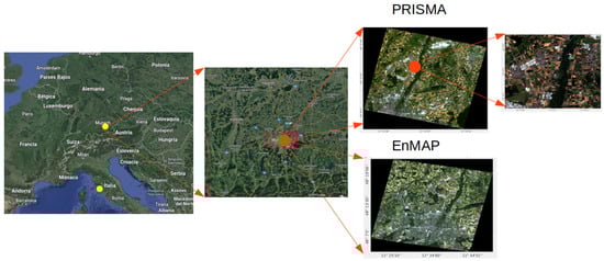
Figure 2.
Zoom in with PRISMA scene at the test site in the North of Munich (Munich-North-Isar, MNI), Germany. EnMAP scene in North of Munich, Germany. The Grosseto and MNI test sites are marked with yellow dots.
2.7.1. PRISMA Acquisition
The PRISMA satellite is operated by the Italian Space Agency (ASI). PRISMA is an imaging spectrometer with 239 contiguous wavebands spanning from 400 to 2500 nm. It offers a spectral sampling interval of less than 11 nm and a full width at half maximum (FWHM) of less than 15 nm. PRISMA provides high-resolution imagery, with a ground spatial resolution of 30 m and a swath width of 30 km. Its capabilities include off-nadir observations of up to ±14.7 degrees.
A PRISMA image was acquired over the MNI agricultural area on 1 August 2020, during a 4-second interval, spanning from 10:25:51 to 10:25:55. This image was downloaded at both the TOA level and the BOA level. The choice of this image is because it was taken 2 years after the validation data collection at exactly the same time of year. The image, at the BOA scale, corresponds to the L2D PRISMA reflectance cube, while the TOA scale image represents the L1 PRISMA radiance cube. These images were obtained in HDF5 format and read using the prismaread tool [85].
A key assumption of the hybrid GPR models is that the training dataset corresponds with that of the imagery to be processed. Therefore, to justify the validity of our approach, in Figure 3 we show two datasets as expressed by the averaged spectra, standard deviation (shaded areas), and min–max ranges. In the first dataset, 70 random vegetation pixels were chosen from the PRISMA image whose spectra are in shades of red, and the second dataset shows the spectra of the RTM used for training, specifically of the CCC variable whose spectra serve as a representative of the other target variables; these spectra are represented in shades of blue. The figures represent the BOA reflectance spectra in plot (A) and the TOA radiance spectra in (B). For both scales, the RTM training data matches closely with that of PRISMA data, thereby supporting the validity of the training data for processing PRISMA imagery. As expected, the RTM training data varies in a wider range, i.e., this variability allows the generation of a valid and generic hybrid model. Altogether, the figures support the usage of the BOA- and TOA-scale training datasets for GPR-based processing of PRISMA imagery.
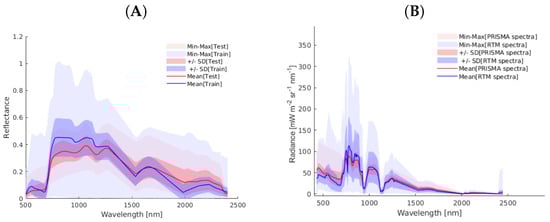
Figure 3.
Comparative statistical analysis of spectral information. (A) Spectral comparison of 70 vegetation pixels from the PRISMA reflectance BOA image (in red) versus the SCOPE-simulated reflectance database for BOA GPR-20PCA models training (in blue). (B) Spectral comparison of 70 vegetation pixels from the PRISMA radiance TOA image (in red) versus the coupled SCOPE-libRadtran simulated reflectance database for training TOA GPR-20PCA models (in blue). [mW msrnm].
2.7.2. EnMAP Acquisition
The German hyperspectral EnMAP sensor is a pushbroom imaging spectrometer with a total of 240 spectral bands divided in the VNIR range (420–1000 nm at 6.5 nm resolution) and SWIR range (900–2450 nm at 10 nm resolution). It offers high radiometric resolution and stability in both spectral ranges. EnMAP provides a swath width of 30 km with a spatial resolution of 30 × 30 m. It supports rapid target review by pointing towards nadir (30 degrees) and can acquire a sweep of 1 km per orbit and a total of 5 km per day.
The models developed in this study were applied to an EnMAP image captured on 28 July 2022. The selection of this image serves a dual purpose. Firstly, it was acquired two years after the PRISMA image described above while retaining the same seasonality. Secondly, it belongs to the same agricultural site in northern Germany. Two different level EnMAP products were downloaded: the L2A BOA reflectance cube and the L1C TOA radiance cube. These EnMAP data files were retrieved from the EnMAP mission portal (https://planning.enmap.org/, accessed on 26 March 2024) in TIF format and read using the QGIS application version 3.26, within the specialised EnMAP BOX package. The TOA image was downloaded in digital number (DN) format and accordingly transformed into radiance data through the gain and offset values included in the metadata .xml file.
Analogous to the PRISMA data, Figure 4 shows the comparison of the BOA and TOA simulated datasets compared to the EnMAP data. For both scales, the RTM training data matches closely with that of the EnMAP data, thereby supporting the validity of the training data for processing EnMAP imagery. As expected, the RTM training dataset varies in a wider range, i.e., this variability allows for the generation of a valid and generic hybrid model. Altogether, the figures support the usage of the BOA- and TOA-scale training datasets for the GPR-based processing of EnMAP imagery.
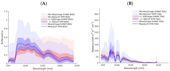
Figure 4.
Comparative statistical analysis of spectral information. (A) Spectral comparison of 70 vegetation pixels from the EnMAP reflectance BOA image (in red) versus the SCOPE-simulated reflectance database for BOA GPR-20PCA models training (in blue). (B) Spectral comparison of 70 vegetation pixels from the EnMAP radiance TOA image (in red) versus the coupled SCOPE–libRadtran simulated reflectance database for training TOA GPR-20PCA models (in blue).
To provide insights into the computational efficiency of our approach, we recorded the execution time on a personal computer (Ubuntu 20.04 LTS 64-bit operating system, Intel i7-9700K CPU 3.60 GHz, 32 GB RAM). Efficient runtime is crucial for operational processing. By optimising both the spectral and sampling domains, we ensured a streamlined and efficient model, even though both models involve 20 functions in their implementation.
3. Results
This section starts with an analysis of the usefulness of using principal component analysis for spectral dimensionality reduction and as an essential part of our hyperspectral workflow. Here, we detail the number of principal components used in the experiments. Also, we provide insights into the importance of each component in the GPR model training at both the BOA and TOA scales. Following that, this section also offers results about the validation of models with acquired in situ data. Finally, trait maps are generated using the BOA- and TOA-based GPR models for both PRISMA and EnMAP imagery, and they are crosscompared.
3.1. PCA and Component Relevance BOA- and TOA-Based GPR Models
We first evaluated the role of PCA spectral dimensionality reduction in the GPR models at the BOA and TOA scales. Figure 5 shows the cumulative explained variability (left axis) and reconstruction error (right axis) as functions of the number of principal components. The total variability was maintained by projecting onto the PCA subspace. The reconstruction accuracy (in terms) was determined after projecting the original data and performing the inverse PCA projection to assess the reconstruction achieved by the low-rank projection. As observed, a subspace of 10 principal components was sufficient to maintain both the explained variability of the original data and the reconstruction accuracy. To be on the safe side, and in agreement with earlier analysis [49], we selected a total of 20 principal components to obtain a projection that satisfied both criteria: the explained variability and the reconstruction error.
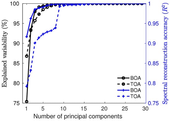
Figure 5.
Dual-axis plot showing the explained variability (in black, left axis) and reconstruction accuracy measured by the coefficient of determination (in blue, right axis) at both BOA and TOA levels.
After the development of the BOA- and TOA-based hybrid GPR models with 20 PCA components, we inspected the relative importance of the 20 components that built the final GPR models (GPR-20PCA models). For each model, the relevance of the components can be demonstrated in a polar plot, i.e., the more outwardly positioned, the more relevant (Figure 6). The relevance of each component has been obtained according to [49]. This value provides numerical evidence regarding the relevance assigned to each component: the bigger the value, the more the relevancy. The polar plots allow us to compare the strengths of the models between the BOA and TOA. Particularly for the LAI and FVC, the BOA components were given more weight than the TOA models, especially in the case of the FVC. Conversely, for the CCC, CWC, and FAPAR the TOA components received slightly more weight than the BOA models. It is noteworthy that the first component was not found in any of the models evaluated among the most important, that is, in none of the cases did the first component preserve most of the spectral variance. Instead, the most relevant components emerged beyond the fifth component. The relevant components all appeared up to component 20. While higher components can capture subtleties relevant to the development of the models, they also capture noise present in the spectral data. At the same time, some components hardly play a relevant role, i.e., they are located in the center of the polar plots. It is worth noting that a more concise data representation can be achieved by retaining only the most relevant components, thus resulting in a reduced data representation while preserving a lower representation error. Yet, we kept the 20 components for all the models to standardise the model comparisons.
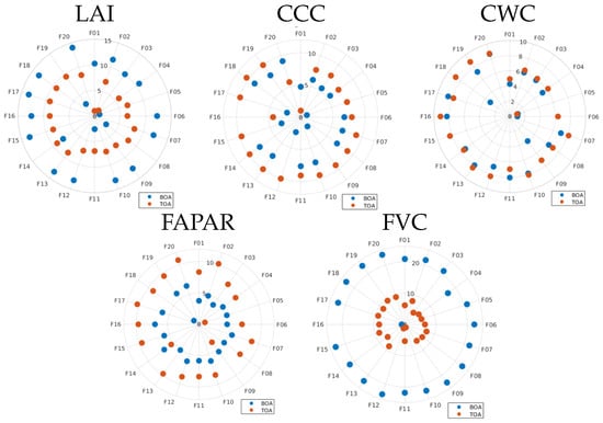
Figure 6.
Polar plots of the principal components (P01–P20) explaining the spectral variability or each variable in the GPR-20PCA models. Distance to origin represents the importance of each component: the more outside, the more important.
3.2. Validation of BOA- and TOA-Based GPR Models
The BOA-based GPR models were used as a reference for evaluating the TOA-based models. They were developed in [49] and were spectrally adapted and retrained so that the models could process both PRISMA and EnMAP imagery, i.e., nonmatching bands were removed. Table 4 summarises the goodness-of-fit statistics, number of samples (N), root mean square error RMSE, relative RMSE (RRMSE), normalised RMSE (NRMSE), , and the computational time (s: seconds) for the algorithm training and model testing. The variables LAI, CCC, and CWC have been accurately validated against in situ data at the BOA scale, with the ranging between 0.69 and 0.82. In situ data were absent for the variables FAPAR and FVC, so they have only been theoretically validated, i.e., against SCOPE simulations. The good validation results give confidence that these models, and subsequently the derived maps, can serve as reference products to evaluate the performance of the TOA-based models.
Table 4.
Goodness-of-fit statistics for canopy variables in Grosseto and MNI in situ datasets (and theoretical results for FVC and FAPAR) achieved with GPR-20PCA models at BOA scale.
Following that, the TOA-based models were also validated. The existing BOA-level validation database was augmented with atmospheric profiles derived from the combined application of the ALG and TOC2TOA toolboxes. The upscaled spectral profiles allowed for validation at the TOA scale. This validation database is only available for the following variables: CCC, CWC, and LAI. For the FAPAR and FVC, we did not have field data for any of the levels, so only theoretical goodness-of-fit results are provided (Table 5). Upon inspecting the validation results, it is encouraging that the TOA validation statistics are similar to those of the BOA, with an improvement for the LAI ( of 0.92) and a slight decline for the other variables, as noted by the error metrics (RMSE, RRMSE, and NRMSE). The results give confidence that the models can be directly applied at the TOA scale. Also, the training time took considerably longer than the BOA models, given the larger training size (1500 samples), which in GPR training times increase cubically. Nevertheless, the testing time (i.e., runtime) is still quasi-instant, thereby implying that full images were processed in the order of minutes.
Table 5.
Goodness-of-fit statistics for canopy variables in Grosseto and MNI in situ data sets (and theoretical results for FVC and FAPAR) achieved with GPR-20PCA models at TOA scale: number of samples (N), RMSE, RRMSE, NRMSE, , and computational time (s: seconds) for algorithm training and model testing.
For a closer comparison of the models’ performances, Figure 7 displays the scatterplots of the BOA- and TOA-based GPR models against corresponding validation data. The plots also provide the same goodness-of-fit statistics, the number of validation samples n, and the equation for the linear fitting line. Overall, the fitting line closely follows a 1:1 line, thereby indicating robust validation. The colour bar, along with the estimates, represents the associated standard deviation (SD), i.e., uncertainty, as produced by the GPR models. It can be noted that the uncertainties are low for the large majority of retrievals. When comparing the BOA against the TOA, it is of interest is that no systematic degradation at the TOA scale can be noted, which suggests the consistency of the TOA models relative to the BOA models. These results thus support the adequacy of the TOA-based GPR models for traits mapping directly at the TOA radiance scale. In the next step, the BOA and TOA models were applied to process the PRISMA and EnMAP imageries.
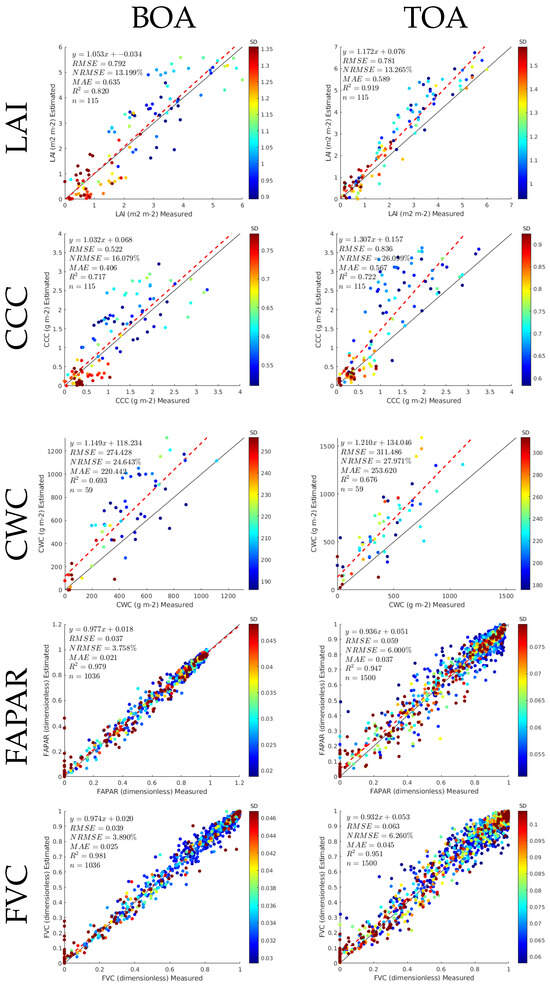
Figure 7.
Scatterplots with goodness-of-fit statistics for the GPR-20PCA models at BOA and TOA levels with validation using in situ data from Grosseto and MNI measurements. In the case of FAPAR and FVC, crossvalidation results are provided (no in situ data are available). The colour bar indicates the standard deviation (SD), i.e., uncertainty, achieved by the GPR models.
3.3. BOA- and TOA-Based Vegetation Trait Mapping Using PRISMA and EnMAP Imagery and Comparison
The hybrid GPR models were applied at both the BOA and TOA levels of the PRISMA and EnMAP imagery acquired in northern Munich to illustrate the mapping application. To avoid anomalies related to the lack of PRISMA L1 geometry and geometric matching between the BOA and TOA images, only a spatial subset of the PRISMA images was processed. The output trait maps were then compared by computing a scatterplot and goodness-of-fit statistics (RMSE, NRMSE, and ). A visualisation analysis allows for the evaluation of the accuracy of the processing surfaces with and without vegetation. Apart from croplands dominating the image, the area is also characterized by strips of natural vegetation along the river and some patches of forest.
3.3.1. PRISMA Mapping Results
The PRISMA image was acquired both at the BOA and TOA levels over the Jolanda di Savoia site. Figure 8 illustrates the results of processing the PRISMA images through the TOA- and BOA-based GPR models for the traits LAI, CCC, CWC, FAPAR, and FVC. A visual inspection of the resulting maps indicates consistency between the vegetated and nonvegetated surfaces mapped at both the BOA and TOA scales. For all traits, the NRMSE relative errors between the BOA- and TOA-based maps were in the same order, around 10–16%. However, the LAI, CCC and CWC suffered from overestimations over the nonvegetation surfaces, such as barren land and water bodies.
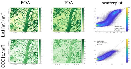
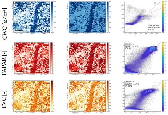
Figure 8.
Results of estimated canopy variables LAI, CCC, CWC, FAPAR, and FVC, for the GPR-20PCA model. The first and second columns show the trait maps retrieved from the PRISMA L2D BOA image and PRISMA L1 TOA image, respectively. The third row illustrates the scatterplots of both maps, the X axis corresponds to the BOA results, and the Y axis corresponds to the TOA results; the scatterplot’s colour bar indicates the relative density of points.
The CWC exhibited the weakest performance in the TOA domain, with pronounced overestimations over nonvegetated surfaces. Conversely, it is worth noting that the FAPAR and FVC yielded comparable BOA- and TOA-based maps, even though the models of these traits were not optimized against in situ data. Both models produced estimates within the 0 to 1 range, and the spatial patterns recovered matched closely between the BOA and TOA retrievals. Furthermore, all traits displayed expected higher values in the vegetated regions, particularly along the riverbanks and areas with trees and dense vegetation. In contrast, the nonvegetated surfaces exhibited lower values or even near-zero values, especially for the FVC and FAPAR. The third column of Figure 8 includes the scatterplots between the maps and the numerical results. It can be noticed that the reached a relatively high value between the maps, thus being greater than for all variables. This encouraging correlation between the BOA and TOA maps supports the suitability of mapping vegetation traits directly at the TOA scale.
3.3.2. EnMAP Mapping Results
To provide a wider comparison of the proposed methodology, the BOA- and TOA-based GPR models were additionally applied to EnMAP L2A and L1C images acquired in the same region located over the south of Munich. A visual inspection of the resulting maps indicates consistency between the vegetated and nonvegetated surfaces, which were consistently mapped at both scales (BOA and TOA). The comparison results achieved in all variables can be considered good, as the between BOA and TOA was above 0.85, and the NRMSE relative errors were between 4 and 11% for all the traits. Furthermore, visual inspection describes consistency between the maps at both levels for all the considered traits. The scatterplots in Figure 9 (right column) demonstrate a strong correlation between the maps and the corresponding numerical values by achieving relatively low values of the RMSE and NRMSE error metrics.
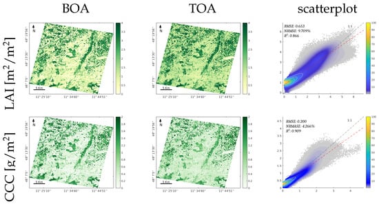

Figure 9.
Mapping of estimated canopy variables LAI, CCC, CWC, FAPAR, and FVC, for the GPR-20PCA models. The first and second columns show the trait maps retrieved from the EnMAP L2A BOA image and the EnMAP L1C TOA image, respectively. The third row illustrates the scatterplots of both maps, the X axis corresponds to the BOA results, and the Y axis corresponds to the TOA results; the scatterplot’s colour bar indicates the relative density of points.
3.3.3. Mapping Runtime
The computational execution time was acquired both from the training and test phases. Table 6 summarises the computational execution time of the hybrid models based on the BOA and TOA for the EnMAP and PRISMA scenes. As can be observed, the computational execution time for the retrievals of the PRISMA image was generally lower than the EnMAP; this is due to its lower size scene in pixels. The PRISMA scene contains pixels and the EnMAP scene contains pixels, thereby affecting the CPU execution time. Regarding the execution time in the training phase, it was higher for the hybrid models based on TOA, since they involved a larger training dataset of 1500 samples (see Table 5), and in the BOA models, they involved 409 samples for the CCC variable, 526 samples for the LAI and CWC variables, and 1036 samples for the FAPAR and FVC (see Table 4). It is worth mentioning that the GPR model used dominated the CPU execution time, thereby having a cubic order concerning the number of samples; this implies a heavier calculation when N grows.
Table 6.
Computational execution time to process the images into trait maps. Times are reported in seconds [s].
4. Discussion
Despite the widespread practice of applying retrieval models to atmospherically corrected images, in this study, we explored the development of hybrid models capable of directly analyzing hyperspectral TOA radiance imagery. Essentially, such an approach saves the atmospheric correction processing time and avoids potential errors derived from this process. This TOA-based retrieval approach has been laid out here in support of the upcoming CHIME and evaluated with the scientific hyperspectral precursor mission data from PRISMA and EnMAP. To the best of our knowledge, this is the first study estimating multiple vegetation traits from satellite hyperspectral radiance data using a hybrid workflow. Though comparison studies at the TOA scale are lacking, our results can be compared against retrievals achieved at the BOA scale. The following sections discuss the key aspects achieved in this study. Firstly, we examine the RTM and sensors’ data comparison (Section 4.1); secondly, we examine the retrieval performance with the hybrid workflow applied to the BOA and TOA (Section 4.2); thirdly, we examine the Gaussian processes regression and delivered uncertainty (Section 4.4); and quarterly, we examine the variable-specific mapping using PRISMA and EnMAP imagery (Section 4.3). Lastly, the limitations and further research opportunities are discussed in Section 4.5).
4.1. RTM and Sensor Data Comparison
When aiming to move towards a routine processing of hyperspectral data into vegetation traits across the globe, the implemented retrieval algorithm has to be accurate, robust, and fast, preferably with the provision of uncertainty intervals alongside the estimates [43]. To this end, hybrid models have been evaluated as the most promising, thereby combining physically based RTMs with the flexibility of machine learning algorithms [44]. In this context, the ability to generate realistic data from RTMs is crucial for developing highly effective hybrid models. This was achieved by both optimizing in the spectral domain, through PCA dimensionality reduction [49], and through optimising the training dataset. In addition to applying a realistic sampling design within the RTM parameter spaces, this can be accomplished by further optimising the selection of RTM training samples through the AL procedure, as has been extensively demonstrated and discussed in previous studies [47,48,49,73]. Using AL supports, we can accomplish the establishment of a representative training dataset, which is the main prerequisite for the successful training of the retrieval models. Furthermore, the RTM spectral output should be configured according to the band settings of the imagery where the hybrid model will be applied to [39,49]. The usage of a proper RTM setting allows for the simulation of diverse, yet realistic vegetation scenarios, which better represent real scenarios. The primary objective of this study was to develop hybrid models tailored to the capabilities of the upcoming CHIME satellite. Since the CHIME mission is still in its development phase and a proven atmospheric correction method is unavailable, we explored the development of hybrid models directly at the TOA scale and benchmarked them against BOA-based models. Anticipating the availability of CHIME data, the developed models were evaluated using PRISMA and EnMAP imagery. PRISMA and EnMAP image spectral bands were resampled to align with the spectral range of previously validated CHIME models, thereby ensuring compatibility with the sensor specifications [49].
Having a consistent band setting between the RTM training and satellite-recorded data at both the BOA and TOA scales, Section 2.7 provided descriptive statistical comparisons of the spectra for both PRISMA and EnMAP sensors to validate their spectral similarity (Figure 3 and Figure 4). These illustrations showcase the similarity between the simulated and satellite-recorded spectra, thereby implying that the hybrid models can correctly interpret and convert the spectral data into vegetation traits both at the BOA and TOA levels.
4.2. Retrieval Performance at BOA and TOA Scales
The hybrid models developed in this study combine the strengths of physical and statistical models to achieve both portability and robustness. At the same time, the PCA dimensionality reduction step ensures optimal exploitation of the spectral domain, while the AL step ensures optimal selection of the RTM training samples [49]. As a novelty compared to previous studies, in this study both optimization steps were applied to the BOA and TOA scales. For the traits LAI, CCC, and CWC, both the BOA and TOA models were adequately validated against field data (e.g., ranging between 0.69 and 0.92). Moreover, a slight tendency emerged favoring superior estimates derived from the TOA scale for the canopy variable LAI. It is noteworthy that previous studies conducted by Estévez et al. [29,35] using Sentinel-2 data also demonstrated superior LAI retrieval performance at the TOA scale as opposed to the BOA scale. At the same time, the BOA validation showed slightly higher accuracies for the other analyzed variables. However, the TOA scale demonstrated comparable accuracy levels, thus highlighting its competitive performance. The high TOA-based accuracies could be attributed to the potential degradation of BOA hyperspectral data quality during the multiple processing stages involved in converting the L1C product to L2A, which could have negatively impacted retrieval accuracy [11].
Related to this topic, hybrid models often add some degree of noise to the training dataset, e.g., [29,35,39,86]. This spectral degradation of the training dataset can lead to an improvement in the validation statistics, as it mitigates the tendency of overfitting the model toward synthetic RTM data. In our TOA-based models, combining canopy simulations with atmospheric simulations might likewise have acted somewhat as a noise perturbation factor of the vegetation RTM spectra, i.e., this perturbation similarly mitigates the tendency of overfitting.
Also, the observed moderate discrepancies between the BOA and TOA and the field validation data require further explanation. On the one hand, these discrepancies may be attributed to the use of different RTMs for the atmospheric simulation versus the atmospheric correction in the PRISMA and EnMAP processors, which causes a net effect similar to radiometric calibration errors. While in this study libRadtran was used to generate the TOA training dataset, both PRISMA’s and EnMAP’s atmospheric corrections are based on MODTRAN [87,88]. This suggests that further work should ensure consistency among the atmospheric RTMs used for the generation of the training dataset and in the atmospheric correction processors. On the other hand, as previously mentioned, the spectral resampling to a common spectral configuration (CHIME) introduces additional noise in the PRISMA/EnMAP images, particularly in the vicinity of gas absorption regions. This noise is enhanced by effects such as spectral calibration errors and smile. Although major absorption bands have been filtered out (Section 2.3) to reduce the impact of this noise, residual HO and O bands were still present in the data and might have contributed to an increased noise level in the data.
4.3. Machine Learning Regression Model and Uncertainty
The work presented here is the natural continuation of a research line that focuses on the development of GPR-based hybrid models e.g., [29,35,36,37,38]. GPR allows for the development of hybrid models with accurate predictions and valuable estimations of uncertainty for each test spectrum. Following the results achieved in Table 4 and Table 5, it can be deduced that GPR achieves good performance along the considered metrics.
The training time for GPR hybrid models is a significant factor to consider. As the training time grows cubically as a function of the training samples [89], it typically exceeds the application time by several orders of magnitude. However, in the context of real-world operational applications, where timely retrieval estimations are paramount, the prediction time emerges as the more critical parameter. GPR hybrid models, despite their relatively lengthy training process, excel in their application performance, thereby enabling them to swiftly process new incoming spectra and rendering them highly suitable for routine global mapping applications. This trade-off between training time and application efficiency makes GPR hybrid models particularly well suited for scenarios demanding the rapid retrieval of new spectra.
Another aspect of GPR that makes it a highly appealing MLRA for operational contexts is its built-in uncertainty estimation. GPR not only provides an estimation but also generates a corresponding normal distribution. This normal distribution is characterized by its standard deviation, which serves as an uncertainty estimate for the mean retrieval value. Uncertainty estimates are crucial for the effective interpretation of GPR model outputs, as they enable per-pixel evaluation of the performance of the model [50]. Furthermore, uncertainty estimations are particularly valuable in operational contexts where models cannot be validated for all locations. For instance, uncertainty information from (future) Copernicus products is usually requested to support the application of the data and products in various contexts, such as policy and climate modelling, e.g., [90]. Therefore, it should be an obligatory part of the provided products.
Here, the uncertainty estimation provided in Figure 7 indicates that our models are more proficient at estimating vegetation traits on spectra where vegetation density is high. Notably, the LAI, CCC, and CWC uncertainties were larger on the left side of the axis. This trend could be attributed to the increasing influence of soil in the spectra of pixels with lower vegetation density. This behavior is supported by the FVC and FAPAR uncertainty values, as these models were optimised and validated only against RTM-generated data (i.e., with less influence of soil in the turbid medium model SCOPE), and their uncertainty estimates appear to be less attributed to vegetation density.
4.4. Variable-Specific Mapping in PRISMA and EnMAP Sensors
Inspecting both the PRISMA- and EnMAP-based trait maps in Figure 8 and Figure 9, it can be concluded that TOA-based mapping is possible for both data sources. Particularly, the FAPAR and FVC led to meaningful maps with strong similarity towards their BOA-based counterparts. At the same time, it is also noteworthy that the PRISMA TOA-based LAI, CCC, and CWC maps were not completely behaving as expected, with a general tendency toward overestimation over nonvegetated surfaces. This can be attributed to various error sources. First, the spectral resampling to CHIME resolution might derive higher errors due to the coarser spectral resolution of PRISMA (∼15 nm) compared to EnMAP (6.5–10 nm). Second, the GPR models were trained by adding bare soil spectra to the training dataset. These soil spectra might not be suitable for the specific image acquisition by PRISMA. This factor warrants consideration during the development of future models.
In the broader context, the efficiency of the models in processing full TOA images within minutes underscores their feasibility for large-scale applications. The consistent mapping results between the BOA and TOA scales, along with the low uncertainties, emphasise the practical utility of these models for real-world applications such as precision agriculture, land cover monitoring, and ecosystem assessment. Discussing the larger implications of our findings, the consistent performance of the TOA-based models across multiple hyperspectral sensors signifies their applicability and scalability. The trait mapping results, particularly for the FAPAR and FVC, hold significance for monitoring vegetation health and productivity. These findings contribute valuable information for environmental monitoring, land management, and policy formulation.
It also deserves remarking that the cropland characteristics at the canopy level were often inferred more accurately from space than leaf-level traits such as the LCC [91]. Our findings for the L1C and L2A scales clearly showed that tendency, which was also supported by a few related studies examining Sentinel-2 data [66,92,93]. Xie et al. [66] suggested that this can be caused by the compensating effects between the LAI and LCC, which could account for the lower retrieval accuracy at the leaf level. The precision with which leaf biochemicals may be retrieved from canopy reflectance may also be influenced by the signal’s intensity or signal propagation, which is primarily determined by structural characteristics like the LAI [94,95].
4.5. Limitations and Further Research Opportunities
Reviewing our research objectives, the developed hybrid GPR models successfully addressed the challenge of canopy trait mapping from hyperspectral imagery at the TOA level. However, a few limitations had to be addressed, and some warrant further exploration to enhance the accuracy and robustness of the retrieval models. For instance, to overcome the lack of in situ observations for the FAPAR and FVC, we increased the number of simulated samples from 500 (as for the LAI, CCC, and CWC) to 1000, thus enhancing the generalisation capability and robustness of the models.
A notable limitation of the study is that only canopy-level traits were mapped. Some initial tests with leaf-level variables showed rather low performance. These findings align with the results of previous studies, thus demonstrating that leaf-level variables are more challenging to retrieve with sufficient accuracy using TOA-based data [35,36]. The superior performance of our canopy-scale retrievals for the CCC and CWC can be attributed to the role of LAI in leaf-to-canopy upscaling. The LAI represents the density of leaves and, as such, the contrast between vegetated and nonvegetated fractions of the surface. Indeed, the LAI is recognized as one of the strongest drivers of spectral variability across the entire VNIR and SWIR spectral range [20].
To further improve model efficiency, follow-up research could investigate potential improvements both in the employed algorithm and the optimization of the number of principal components. Alternative machine learning approaches could be explored to enhance the obtained results, such as employing large-scale formulations of GPR [46,96]. Multioutput regression models might also ensure physical correlations between the traits, thereby enhancing the robustness of the models [97]. Other methods such as multifidelity [98] can improve the efficiency of the retrieval while improving the accuracy of the output product. Additionally, the use of more advanced three-dimensional RTMs, such as DART e.g., [99] could be leveraged to generate more data and feed these large-scale approaches to construct more accurate models. To further broaden the applicability and implementation on other hyperspectral missions and in a range of geographical settings would significantly enhance the generalisability of the models e.g., [100]. Additionally, incorporating additional trait variables would provide a more comprehensive understanding of the vegetation dynamics and their underlying mechanisms across the globe e.g., [101].
Another relevant aspect of research is applying the developed models to hyperspectral time series data. These, however, are not yet available from current missions. This would allow us to track the temporal evolution of vegetation traits in various ecosystems. Additionally, expanding the scope of the study to include different crop types within the study region, and their various phenological stages would further enhance its value. Also, investing in the portability of the models would be beneficial to further advance this work. In the upcoming era of big data, it is expected that these TOA-based hybrid GPR models can be implemented into cloud computing platforms [102], thus opening the processing chain to the broader community without the need to download TOA radiance imagery. Finally, it is important to note that all the developments and models presented here can be relatively easily reproduced. The satellite data used in the study are open (upon registration), and the hybrid models can be replicated through the ALG tool and ARTMO toolbox (both downloadable at http://artmotoolbox.com/ (accessed on 26 March 2024)). Likewise, the provided tools facilitate customization for any applicable sensor by enabling the training of GPR models with resampled TOA spectral data tailored to the desired spectral band configuration.
5. Conclusions
This study successfully demonstrated the feasibility of directly retrieving vegetation traits from TOA radiance data using machine learning GPR models, thereby eliminating the need for atmospheric correction. A hybrid modelling approach was employed combining the vegetation radiative transfer model (SCOPE) with the atmospheric radiative transfer model (libRadtran) to train GPR directly on TOA radiance simulations. This enabled the retrieval of a comprehensive suite of vegetation canopy traits, including the LAI, CCC, CWC, FAPAR, and FVC. The developed TOA- and BOA-based hybrid GPR models exhibited promising performance in retrieving these traits, thereby achieving good to optimal accuracies when compared to in situ data ( values ranging between 0.68 and 0.95). The TOA models demonstrated slightly superior LAI accuracies compared to the BOA models, thus suggesting their potential for direct trait retrieval at the TOA level. To subsequently evaluate the hybrid models’ applicability, they were applied to PRISMA and EnMAP imagery, thus resulting in consistent landscape trait maps between the TOA and BOA levels. This study lays the foundation for the further development and refinement of physically based machine learning hybrid models, thereby paving the way for robust vegetation trait estimation directly at the TOA level. This advancement will streamline global trait mapping applications, particularly within the context of the upcoming operational mission CHIME.
Author Contributions
Conceptualization, J.E. and J.V. (Jochem Verrelst); Methodology, A.B.P.-V., K.B., J.E., J.V. (Jorge Vicent) and J.V. (Jochem Verrelst); Software, A.B.P.-V. and J.L.G.; Validation, A.B.P.-V., J.L.G., J.E. and J.V. (Jorge Vicent); Formal analysis, J.L.G., A.P.-S., S.V.W. and J.V. (Jochem Verrelst); Investigation, J.V. (Jorge Vicent) and J.V. (Jochem Verrelst); Data curation, A.B.P.-V., J.V. (Jorge Vicent) and J.V. (Jochem Verrelst); Writing—original draft, A.B.P.-V., K.B., J.E., A.P.-S., S.V.W. and J.V. (Jochem Verrelst); Writing—review & editing, A.B.P.-V., J.L.G., J.V. (Jorge Vicent), A.P.-S., S.V.W. and J.V. (Jochem Verrelst); Visualization, A.B.P.-V.; Supervision, A.P.-S., S.V.W. and J.V. (Jochem Verrelst); Project administration, J.V. (Jochem Verrelst); Funding acquisition, J.V. (Jochem Verrelst). All authors have read and agreed to the published version of the manuscript.
Funding
This research was funded by the European Research Council (ERC) under the projects SENTIFLEX (#755617) and FLEXINEL (#101086622). The views and opinions expressed are, however, those of the author(s) only and do not necessarily reflect those of the European Union or the European Research Council. Neither the European Union nor the granting authority can be held responsible for them. A.B.P. and S.V.W. were supported by the European Research Council (ERC) under the ERC-2021-STG project PHOTOFLUX (grant agreement no. 101041768).
Data Availability Statement
Data sharing is not applicable to this article.
Conflicts of Interest
Author Jorge Vicent was employed by the company Magellium. The remaining authors declare that the research was conducted in the absence of any commercial or financial relationships that could be construed as a potential conflict of interest.
References
- Weiss, M.; Jacob, F.; Duveiller, G. Remote sensing for agricultural applications: A meta-review. Remote Sens. Environ. 2020, 236, 111402. [Google Scholar] [CrossRef]
- Hank, T.B.; Berger, K.; Bach, H.; Clevers, J.G.P.W.; Gitelson, A.; Zarco-Tejada, P.J.; Mauser, W. Spaceborne Imaging Spectroscopy for Sustainable Agriculture: Contributions and Challenges. Surv. Geophys. 2019, 551, 515–551. [Google Scholar] [CrossRef]
- Celesti, M.; Rast, M.; Adams, J.; Boccia, V.; Gascon, F.; Isola, C.; Nieke, J. The Copernicus Hyperspectral Imaging Mission for the Environment (Chime): Status and Planning. In Proceedings of the IGARSS 2022—2022 IEEE International Geoscience and Remote Sensing Symposium, Kuala Lumpur, Malaysia, 17–22 July 2022; IEEE: Piscataway, NJ, USA, 2022; pp. 5011–5014. [Google Scholar]
- Ustin, S.L.; Middleton, E.M. Current and near-term advances in Earth observation for ecological applications. Ecol. Process. 2021, 10, 1. [Google Scholar] [CrossRef] [PubMed]
- Verrelst, J.; Halabuk, A.; Atzberger, C.; Hank, T.; Steinhauser, S.; Berger, K. A comprehensive survey on quantifying non-photosynthetic vegetation cover and biomass from imaging spectroscopy. Ecol. Indic. 2023, 155, 110911. [Google Scholar] [CrossRef]
- Gao, B.C.; Montes, M.J.; Davis, C.O.; Goetz, A.F. Atmospheric correction algorithms for hyperspectral remote sensing data of land and ocean. Remote Sens. Environ. 2009, 113, S17–S24. [Google Scholar] [CrossRef]
- Main-Knorn, M.; Pflug, B.; Louis, J.; Debaecker, V.; Müller-Wilm, U.; Gascon, F. Sen2Cor for Sentinel-2. In Proceedings of the Image and Signal Processing for Remote Sensing XXIII, Warsaw, Poland, 11–14 September 2017; Volume 10427, p. 3. [Google Scholar]
- Thompson, D.R.; Natraj, V.; Green, R.O.; Helmlinger, M.C.; Gao, B.C.; Eastwood, M.L. Optimal estimation for imaging spectrometer atmospheric correction. Remote Sens. Environ. 2018, 216, 355–373. [Google Scholar] [CrossRef]
- Vermote, E.F.; Kotchenova, S. Atmospheric correction for the monitoring of land surfaces. J. Geophys. Res. Atmos. 2008, 113, 012001. [Google Scholar] [CrossRef]
- Callieco, F.; Dell’Acqua, F. A comparison between two radiative transfer models for atmospheric correction over a wide range of wavelengths. Int. J. Remote Sens. 2011, 32, 1357–1370. [Google Scholar] [CrossRef]
- Thompson, D.; Guanter, L.; Berk, A.; Gao, B.C.; Richter, R.; Schläpfer, D.; Thome, K. Retrieval of Atmospheric Parameters and Surface Reflectance from Visible and Shortwave Infrared Imaging Spectroscopy Data. Surv. Geophys. 2019, 40, 333–360. [Google Scholar] [CrossRef]
- Laurent, V.; Verhoef, W.; Clevers, J.; Schaepman, M. Estimating forest variables from top-of-atmosphere radiance satellite measurements using coupled radiative transfer models. Remote Sens. Environ. 2011, 115, 1043–1052. [Google Scholar] [CrossRef]
- Wang, R.; Gamon, J.A.; Moore, R.; Zygielbaum, A.I.; Arkebauer, T.J.; Perk, R.; Leavitt, B.; Cogliati, S.; Wardlow, B.; Qi, Y. Errors associated with atmospheric correction methods for airborne imaging spectroscopy: Implications for vegetation indices and plant traits. Remote Sens. Environ. 2021, 265, 112663. [Google Scholar] [CrossRef]
- Martins, V.S.; Barbosa, C.C.F.; De Carvalho, L.A.S.; Jorge, D.S.F.; Lobo, F.d.L.; Novo, E.M.L.d.M. Assessment of atmospheric correction methods for Sentinel-2 MSI images applied to Amazon floodplain lakes. Remote Sens. 2017, 9, 322. [Google Scholar] [CrossRef]
- Ilori, C.O.; Pahlevan, N.; Knudby, A. Analyzing performances of different atmospheric correction techniques for Landsat 8: Application for coastal remote sensing. Remote Sens. 2019, 11, 469. [Google Scholar] [CrossRef]
- Vicent, J.; Sabater, N.; Verrelst, J.; Alonso, L.; Moreno, J. Assessment of Approximations in Aerosol Optical Properties and Vertical Distribution into FLEX Atmospherically-Corrected Surface Reflectance and Retrieved Sun-Induced Fluorescence. Remote Sens. 2017, 9, 675. [Google Scholar] [CrossRef]
- Nazeer, M.; Ilori, C.O.; Bilal, M.; Nichol, J.E.; Wu, W.; Qiu, Z.; Gayene, B.K. Evaluation of atmospheric correction methods for low to high resolutions satellite remote sensing data. Atmos. Res. 2021, 249, 105308. [Google Scholar] [CrossRef]
- Katkovsky, L.V.; Martinov, A.O.; Siliuk, V.A.; Ivanov, D.A.; Kokhanovsky, A.A. Fast atmospheric correction method for hyperspectral data. Remote Sens. 2018, 10, 1698. [Google Scholar] [CrossRef]
- Fang, H.; Liang, S. Retrieving leaf area index with a neural network method: Simulation and validation. IEEE Trans. Geosci. Remote Sens. 2003, 41, 2052–2062. [Google Scholar] [CrossRef]
- Verrelst, J.; Vicent, J.; Rivera-Caicedo, J.P.; Lumbierres, M.; Morcillo-Pallarés, P.; Moreno, J. Global Sensitivity Analysis of Leaf-Canopy-Atmosphere RTMs: Implications for Biophysical Variables Retrieval from Top-of-Atmosphere Radiance Data. Remote Sens. 2019, 11, 1923. [Google Scholar] [CrossRef] [PubMed]
- Lauvernet, C.; Baret, F.; Hascoët, L.; Buis, S.; Le Dimet, F.X. Multitemporal-patch ensemble inversion of coupled surface–atmosphere radiative transfer models for land surface characterization. Remote Sens. Environ. 2008, 112, 851–861. [Google Scholar] [CrossRef]
- Laurent, V.; Verhoef, W.; Clevers, J.; Schaepman, M. Inversion of a coupled canopy-atmosphere model using multi-angular top-of-atmosphere radiance data: A forest case study. Remote Sens. Environ. 2011, 115, 2603–2612. [Google Scholar] [CrossRef]
- Laurent, V.; Verhoef, W.; Damm, A.; Schaepman, M.; Clevers, J. A Bayesian object-based approach for estimating vegetation biophysical and biochemical variables from APEX at-sensor radiance data. Remote Sens. Environ. 2013, 139, 6–17. [Google Scholar] [CrossRef]
- Laurent, V.C.; Schaepman, M.E.; Verhoef, W.; Weyermann, J.; Chávez, R.O. Bayesian object-based estimation of LAI and chlorophyll from a simulated Sentinel-2 top-of-atmosphere radiance image. Remote Sens. Environ. 2014, 140, 318–329. [Google Scholar] [CrossRef]
- Shi, H.; Xiao, Z.; Liang, S.; Zhang, X. Consistent estimation of multiple parameters from MODIS top of atmosphere reflectance data using a coupled soil-canopy-atmosphere radiative transfer model. Remote Sens. Environ. 2016, 184, 40–57. [Google Scholar] [CrossRef]
- Shi, H.; Xiao, Z.; Liang, S.; Ma, H. A method for consistent estimation of multiple land surface parameters from MODIS top-of-atmosphere time series data. IEEE Trans. Geosci. Remote Sens. 2017, 55, 5158–5173. [Google Scholar] [CrossRef]
- Bayat, B.; van der Tol, C.; Verhoef, W. Retrieval of land surface properties from an annual time series of Landsat TOA radiances during a drought episode using coupled radiative transfer models. Remote Sens. Environ. 2020, 238, 110917. [Google Scholar] [CrossRef]
- Mousivand, A.; Menenti, M.; Gorte, B.; Verhoef, W. Multi-temporal, multi-sensor retrieval of terrestrial vegetation properties from spectral-directional radiometric data. Remote Sens. Environ. 2015, 158, 311–330. [Google Scholar] [CrossRef]
- Estévez, J.; Vicent, J.; Rivera-Caicedo, J.P.; Morcillo-Pallarés, P.; Vuolo, F.; Sabater, N.; Camps-Valls, G.; Moreno, J.; Verrelst, J. Gaussian processes retrieval of LAI from Sentinel-2 top-of-atmosphere radiance data. ISPRS J. Photogramm. Remote Sens. 2020, 167, 289–304. [Google Scholar] [CrossRef]
- Verhoef, W.; Bach, H. Coupled soil–leaf-canopy and atmosphere radiative transfer modeling to simulate hyperspectral multi-angular surface reflectance and TOA radiance data. Remote Sens. Environ. 2007, 109, 166–182. [Google Scholar] [CrossRef]
- Berk, A.; Anderson, G.; Acharya, P.; Bernstein, L.; Muratov, L.; Lee, J.; Fox, M.; Adler-Golden, S.; Chetwynd, J.; Hoke, M.; et al. MODTRANTM5: 2006 Update. In Proceedings of the SPIE 6233, Algorithms and Technologies for Multispectral, Hyperspectral, and Ultraspectral Imagery XII, Kissimmee, FL, USA, 17–20 April 2006. [Google Scholar]
- Vermote, E.; Tanré, D.; Deuzé, J.; Herman, M.; Morcrette, J.J. Second simulation of the satellite signal in the solar spectrum, 6S: An overview. IEEE Trans. Geosci. Remote Sens. 1997, 35, 675–686. [Google Scholar] [CrossRef]
- Emde, C.; Buras-Schnell, R.; Kylling, A.; Mayer, B.; Gasteiger, J.; Hamann, U.; Kylling, J.; Richter, B.; Pause, C.; Dowling, T.; et al. The libRadtran software package for radiative transfer calculations (version 2.0.1). Geosci. Model Dev. 2016, 9, 1647–1672. [Google Scholar] [CrossRef]
- Vicent, J.; Verrelst, J.; Sabater, N.; Alonso, L.; Rivera-Caicedo, J.P.; Martino, L.; Muñoz-Marí, J.; Moreno, J. Comparative analysis of atmospheric radiative transfer models using the Atmospheric Look-up table Generator (ALG) toolbox (version 2.0). Geosci. Model Dev. 2020, 13, 1945–1957. [Google Scholar] [CrossRef]
- Estévez, J.; Berger, K.; Vicent, J.; Rivera-Caicedo, J.P.; Wocher, M.; Verrelst, J. Top-of-Atmosphere Retrieval of Multiple Crop Traits Using Variational Heteroscedastic Gaussian Processes within a Hybrid Workflow. Remote Sens. 2021, 13, 1589. [Google Scholar] [CrossRef]
- Estévez, J.; Salinero-Delgado, M.; Berger, K.; Pipia, L.; Rivera-Caicedo, J.P.; Wocher, M.; Reyes-Muñoz, P.; Tagliabue, G.; Boschetti, M.; Verrelst, J. Gaussian processes retrieval of crop traits in Google Earth Engine based on Sentinel-2 top-of-atmosphere data. Remote Sens. Environ. 2022, 273, 112958. [Google Scholar] [CrossRef]
- Reyes-Muñoz, P.; Pipia, L.; Salinero-Delgado, M.; Belda, S.; Berger, K.; Estévez, J.; Morata, M.; Rivera-Caicedo, J.P.; Verrelst, J. Quantifying Fundamental Vegetation Traits over Europe Using the Sentinel-3 OLCI Catalogue in Google Earth Engine. Remote Sens. 2022, 14, 1347. [Google Scholar] [CrossRef]
- Kovács, D.D.; Reyes-Muñoz, P.; Salinero-Delgado, M.; Mészáros, V.I.; Berger, K.; Verrelst, J. Cloud-Free Global Maps of Essential Vegetation Traits Processed from the TOA Sentinel-3 Catalogue in Google Earth Engine. Remote Sens. 2023, 15, 3404. [Google Scholar] [CrossRef]
- De Grave, C.; Verrelst, J.; Morcillo-Pallarés, P.; Pipia, L.; Rivera-Caicedo, J.P.; Amin, E.; Belda, S.; Moreno, J. Quantifying vegetation biophysical variables from the Sentinel-3/FLEX tandem mission: Evaluation of the synergy of OLCI and FLORIS data sources. Remote Sens. Environ. 2020, 251, 112101. [Google Scholar] [CrossRef]
- Salinero-Delgado, M.; Estévez, J.; Pipia, L.; Belda, S.; Berger, K.; Paredes Gómez, V.; Verrelst, J. Monitoring Cropland Phenology on Google Earth Engine Using Gaussian Process Regression. Remote Sens. 2021, 14, 146. [Google Scholar] [CrossRef]
- Caballero, G.; Pezzola, A.; Winschel, C.; Casella, A.; Sanchez Angonova, P.; Rivera-Caicedo, J.P.; Berger, K.; Verrelst, J.; Delegido, J. Seasonal mapping of irrigated winter wheat traits in Argentina with a hybrid retrieval workflow using sentinel-2 imagery. Remote Sens. 2022, 14, 4531. [Google Scholar] [CrossRef]
- Wocher, M.; Berger, K.; Verrelst, J.; Hank, T. Retrieval of carbon content and biomass from hyperspectral imagery over cultivated areas. ISPRS J. Photogramm. Remote Sens. 2022, 193, 104–114. [Google Scholar] [CrossRef] [PubMed]
- Verrelst, J.; Camps-Valls, G.; Muñoz Marí, J.; Rivera, J.; Veroustraete, F.; Clevers, J.; Moreno, J. Optical remote sensing and the retrieval of terrestrial vegetation bio-geophysical properties—A review. ISPRS J. Photogramm. Remote Sens. 2015, 108, 273–290. [Google Scholar] [CrossRef]
- Verrelst, J.; Malenovskỳ, Z.; Van der Tol, C.; Camps-Valls, G.; Gastellu-Etchegorry, J.P.; Lewis, P.; North, P.; Moreno, J. Quantifying vegetation biophysical variables from imaging spectroscopy data: A review on retrieval methods. Surv. Geophys. 2019, 40, 589–629. [Google Scholar] [CrossRef]
- Abdelbaki, A.; Udelhoven, T. A Review of Hybrid Approaches for Quantitative Assessment of Crop Traits Using Optical Remote Sensing: Research Trends and Future Directions. Remote Sens. 2022, 14, 3515. [Google Scholar] [CrossRef]
- Rasmussen, C.E.; Williams, C.K.I. Gaussian Processes for Machine Learning; The MIT Press: New York, NY, USA, 2006. [Google Scholar]
- Verrelst, J.; Rivera-Caicedo, J.P.; Reyes-Muñoz, P.; Morata, M.; Amin, E.; Tagliabue, G.; Panigada, C.; Hank, T.; Berger, K. Mapping landscape canopy nitrogen content from space using PRISMA data. ISPRS J. Photogramm. Remote Sens. 2021, 178, 382–395. [Google Scholar] [CrossRef]
- Berger, K.; Rivera Caicedo, J.P.; Martino, L.; Wocher, M.; Hank, T.; Verrelst, J. A Survey of Active Learning for Quantifying Vegetation Traits from Terrestrial Earth Observation Data. Remote Sens. 2021, 13, 287. [Google Scholar] [CrossRef]
- Pascual-Venteo, A.B.; Portalés, E.; Berger, K.; Tagliabue, G.; Garcia, J.L.; Pérez-Suay, A.; Rivera-Caicedo, J.P.; Verrelst, J. Prototyping Crop Traits Retrieval Models for CHIME: Dimensionality Reduction Strategies Applied to PRISMA Data. Remote Sens. 2022, 14, 2448. [Google Scholar] [CrossRef]
- Verrelst, J.; Rivera, J.P.; Moreno, J.; Camps-Valls, G. Gaussian processes uncertainty estimates in experimental Sentinel-2 LAI and leaf chlorophyll content retrieval. ISPRS J. Photogramm. Remote Sens. 2013, 86, 157–167. [Google Scholar] [CrossRef]
- Loizzo, R.; Daraio, M.; Guarini, R.; Longo, F.; Lorusso, R.; Dini, L.; Lopinto, E. Prisma Mission Status and Perspective. In Proceedings of the IGARSS 2019—2019 IEEE International Geoscience and Remote Sensing Symposium, Yokohama, Japan, 28 July–2 August 2019; pp. 4503–4506. [Google Scholar] [CrossRef]
- Guanter, L.; Kaufmann, H.; Segl, K.; Foerster, S.; Rogass, C.; Chabrillat, S.; Kuester, T.; Hollstein, A.; Rossner, G.; Chlebek, C.; et al. The EnMAP Spaceborne Imaging Spectroscopy Mission for Earth Observation. Remote Sens. 2015, 7, 8830–8857. [Google Scholar] [CrossRef]
- National Academies of Sciences, Engineering, and Medicine. Thriving on Our Changing Planet: A Decadal Strategy for Earth Observation from Space; The National Academies Press: Washington, DC, USA, 2018. [Google Scholar] [CrossRef]
- Van der Tol, C.; Berry, J.A.; Campbell, P.K.E.; Rascher, U. Models of fluorescence and photosynthesis for interpreting measurements of solar-induced chlorophyll fluorescence. J. Geophys. Res. Biogeosci. 2014, 119, 2312–2327. [Google Scholar] [CrossRef]
- Verrelst, J.; Romijn, E.; Kooistra, L. Mapping vegetation density in a heterogeneous river floodplain ecosystem using pointable CHRIS/PROBA data. Remote Sens. 2012, 4, 2866–2889. [Google Scholar] [CrossRef]
- Vicent, J.; Sabater, N.; Alonso, L.; Verrelst, J.; Moreno, J. Alg: A Toolbox for the Generation of Look-Up tables Based on Atmospheric Radiative Transfer Models. In Proceedings of the 2018 9th Workshop on Hyperspectral Image and Signal Processing: Evolution in Remote Sensing (WHISPERS), Amsterdam, The Netherlands, 23–26 September 2018; pp. 1–5. [Google Scholar] [CrossRef]
- Mayer, B.; Kylling, A. Technical note: The libRadtran software package for radiative transfer calculations—description and examples of use. Atmos. Chem. Phys. 2005, 5, 1855–1877. [Google Scholar] [CrossRef]
- Yang, P.; Prikaziuk, E.; Verhoef, W.; van der Tol, C. SCOPE 2.0: A model to simulate vegetated land surface fluxes and satellite signals. Geosci. Model Dev. 2021, 14, 4697–4712. [Google Scholar] [CrossRef]
- Verhoef, W.; van der Tol, C.; Middleton, E.M. Hyperspectral radiative transfer modeling to explore the combined retrieval of biophysical parameters and canopy fluorescence from FLEX – Sentinel-3 tandem mission multi-sensor data. Remote Sens. Environ. 2018, 204, 942–963. [Google Scholar] [CrossRef]
- Yang, P.; van der Tol, C.; Yin, T.; Verhoef, W. The SPART model: A soil-plant-atmosphere radiative transfer model for satellite measurements in the solar spectrum. Remote Sens. Environ. 2020, 247, 111870. [Google Scholar] [CrossRef]
- Féret, J.B.; Berger, K.; De Boissieu, F.; Malenovskỳ, Z. PROSPECT-PRO for estimating content of nitrogen-containing leaf proteins and other carbon-based constituents. Remote Sens. Environ. 2021, 252, 112173. [Google Scholar] [CrossRef]
- Vilfan, N.; van der Tol, C.; Muller, O.; Rascher, U.; Verhoef, W. Fluspect-B: A model for leaf fluorescence, reflectance and transmittance spectra. Remote Sens. Environ. 2016, 186, 596–615. [Google Scholar] [CrossRef]
- Verhoef, W. Light scattering by leaf layers with application to canopy reflectance modeling: The SAIL model. Remote Sens. Environ. 1984, 16, 125–141. [Google Scholar] [CrossRef]
- Lichtenthaler, H.K. Vegetation Stress: An Introduction to the Stress Concept in Plants. J. Plant Physiol. 1996, 148, 4–14. [Google Scholar] [CrossRef]
- Pavlović, D.; Nikolić, B.; Đurović, S.; Waisi, H.; Anđelković, A.; Marisavljević, D. Chlorophyll as a measure of plant health: Agroecological aspects. Pestic. I Fitomedicina 2014, 29, 21–34. [Google Scholar] [CrossRef]
- Xie, Q.; Dash, J.; Huete, A.; Jiang, A.; Yin, G.; Ding, Y.; Peng, D.; Hall, C.C.; Brown, L.; Shi, Y.; et al. Retrieval of crop biophysical parameters from Sentinel-2 remote sensing imagery. Int. J. Appl. Earth Obs. Geoinf. 2019, 80, 187–195. [Google Scholar] [CrossRef]
- Berger, K.; Atzberger, C.; Danner, M.; D’Urso, G.; Mauser, W.; Vuolo, F.; Hank, T. Evaluation of the PROSAIL model capabilities for future hyperspectral model environments: A review study. Remote Sens. 2018, 10, 85. [Google Scholar] [CrossRef]
- García-Haro, F.J.; Campos-Taberner, M.; Munoz-Mari, J.; Laparra, V.; Camacho, F.; Sanchez-Zapero, J.; Camps-Valls, G. Derivation of global vegetation biophysical parameters from EUMETSAT Polar System. ISPRS J. Photogramm. Remote Sens. 2018, 139, 57–74. [Google Scholar] [CrossRef]
- Rivera-Caicedo, J.P.; Verrelst, J.; Muñoz-Marí, J.; Camps-Valls, G.; Moreno, J. Hyperspectral dimensionality reduction for biophysical variable statistical retrieval. ISPRS J. Photogramm. Remote Sens. 2017, 132, 88–101. [Google Scholar] [CrossRef]
- Verrelst, J.; Rivera, J.P.; Veroustraete, F.; Muñoz-Marí, J.; Clevers, J.G.; Camps-Valls, G.; Moreno, J. Experimental Sentinel-2 LAI estimation using parametric, non-parametric and physical retrieval methods—A comparison. ISPRS J. Photogramm. Remote Sens. 2015, 108, 260–272. [Google Scholar] [CrossRef]
- Verger, A.; Baret, F.; Camacho, F. Optimal modalities for radiative transfer-neural network estimation of canopy biophysical characteristics: Evaluation over an agricultural area with CHRIS/PROBA observations. Remote Sens. Environ. 2011, 115, 415–426. [Google Scholar] [CrossRef]
- Bacour, C.; Baret, F.; Béal, D.; Weiss, M.; Pavageau, K. Neural network estimation of LAI, fAPAR, fCover and LAI×Cab, from top of canopy MERIS reflectance data: Principles and validation. Remote Sens. Environ. 2006, 105, 313–325. [Google Scholar] [CrossRef]
- Verrelst, J.; Dethier, S.; Rivera, J.P.; Munoz-Mari, J.; Camps-Valls, G.; Moreno, J. Active Learning Methods for Efficient Hybrid Biophysical Variable Retrieval. IEEE Geosci. Remote Sens. Lett. 2016, 13, 1012–1016. [Google Scholar] [CrossRef]
- Verrelst, J.; Berger, K.; Rivera-Caicedo, J.P. Intelligent Sampling for Vegetation Nitrogen Mapping Based on Hybrid Machine Learning Algorithms. IEEE Geosci. Remote Sens. Lett. 2021, 18, 2038–2042. [Google Scholar] [CrossRef]
- Verrelst, J.; Alonso, L.; Camps-Valls, G.; Delegido, J.; Moreno, J. Retrieval of vegetation biophysical parameters using Gaussian process techniques. IEEE Trans. Geosci. Remote Sens. 2012, 50, 1832–1843. [Google Scholar] [CrossRef]
- Verrelst, J.; Alonso, L.; Rivera Caicedo, J.; Moreno, J.; Camps-Valls, G. Gaussian Process Retrieval of Chlorophyll Content From Imaging Spectroscopy Data. IEEE J. Sel. Top. Appl. Earth Obs. Remote Sens. 2013, 6, 867–874. [Google Scholar] [CrossRef]
- Camps-Valls, G.; Verrelst, J.; Munoz-Mari, J.; Laparra, V.; Mateo-Jimenez, F.; Gomez-Dans, J. A survey on Gaussian processes for earth-observation data analysis: A comprehensive investigation. IEEE Geosci. Remote Sens. Mag. 2016, 4, 58–78. [Google Scholar] [CrossRef]
- Jolliffe, I.T.; Cadima, J. Principal component analysis: A review and recent developments. Philos. Trans. R. Soc. A Math. Phys. Eng. Sci. 2016, 374, 20150202. [Google Scholar] [CrossRef]
- Wocher, M.; Berger, K.; Danner, M.; Mauser, W.; Hank, T. Physically-based retrieval of canopy equivalent water thickness using hyperspectral data. Remote Sens. 2018, 10, 1924. [Google Scholar] [CrossRef]
- Danner, M.; Berger, K.; Wocher, M.; Mauser, W.; Hank, T. Fitted PROSAIL parameterization of leaf inclinations, water content and brown pigment content for winter wheat and maize canopies. Remote Sens. 2019, 11, 1150. [Google Scholar] [CrossRef]
- Candiani, G.; Tagliabue, G.; Panigada, C.; Verrelst, J.; Picchi, V.; Rivera Caicedo, J.P.; Boschetti, M. Evaluation of Hybrid Models to Estimate Chlorophyll and Nitrogen Content of Maize Crops in the Framework of the Future CHIME Mission. Remote Sens. 2022, 14, 1792. [Google Scholar] [CrossRef]
- Jonckheere, I.; Fleck, S.; Nackaerts, K.; Muys, B.; Coppin, P.; Weiss, M.; Baret, F. Review of methods for in situ leaf area index determination Part I. Theories, sensors and hemispherical photography. Agric. For. Meteorol. 2004, 121, 19–35. [Google Scholar] [CrossRef]
- Ryu, Y.; Nilson, T.; Kobayashi, H.; Sonnentag, O.; Law, B.E.; Baldocchi, D.D. On the correct estimation of effective leaf area index: Does it reveal information on clumping effects? Agric. For. Meteorol. 2010, 150, 463–472. [Google Scholar] [CrossRef]
- Siegmann, B.; Alonso, L.; Celesti, M.; Cogliati, S.; Colombo, R.; Damm, A.; Douglas, S.; Guanter, L.; Hanuš, J.; Kataja, K.; et al. The High-Performance Airborne Imaging Spectrometer HyPlant—From Raw Images to Top-of-Canopy Reflectance and Fluorescence Products: Introduction of an Automatized Processing Chain. Remote Sens. 2019, 11, 2760. [Google Scholar] [CrossRef]
- Busetto, L.; Ranghetti, L. Prismaread: A Tool for Facilitating Access and Analysis of PRISMA L1/L2 Hyperspectral Imagery v1.0.0. 2020. Available online: https://irea-cnr-mi.github.io/prismaread/ (accessed on 26 March 2024).
- Gallo, I.; Boschetti, M.; Rehman, A.U.; Candiani, G. Self-Supervised Convolutional Neural Network Learning in a Hybrid Approach Framework to Estimate Chlorophyll and Nitrogen Content of Maize from Hyperspectral Images. Remote Sens. 2023, 15, 4765. [Google Scholar] [CrossRef]
- Bachmann, M.; Alonso, K.; Carmona, E.; Gerasch, B.; Habermeyer, M.; Holzwarth, S.; Krawczyk, H.; Langheinrich, M.; Marshall, D.; Pato, M.; et al. Analysis-ready data from hyperspectral sensors—the design of the enmap card4l-sr data product. Remote Sens. 2021, 13, 4536. [Google Scholar] [CrossRef]
- Pellegrino, A.; Fabbretto, A.; Bresciani, M.; de Lima, T.M.A.; Braga, F.; Pahlevan, N.; Brando, V.E.; Kratzer, S.; Gianinetto, M.; Giardino, C. Assessing the Accuracy of PRISMA Standard Reflectance Products in Globally Distributed Aquatic Sites. Remote Sens. 2023, 15, 2163. [Google Scholar] [CrossRef]
- Barber, D. Bayesian Reasoning and Machine Learning; Cambridge University Press: Cambridge, UK, 2012. [Google Scholar]
- Merchant, C.J.; Paul, F.; Popp, T.; Ablain, M.; Bontemps, S.; Defourny, P.; Hollmann, R.; Lavergne, T.; Laeng, A.; de Leeuw, G.; et al. Uncertainty information in climate data records from Earth observation. Earth Syst. Sci. Data 2017, 9, 511–527. [Google Scholar] [CrossRef]
- Li, W.; Li, D.; Liu, S.; Baret, F.; Ma, Z.; He, C.; Warner, T.A.; Guo, C.; Cheng, T.; Zhu, Y.; et al. RSARE: A physically-based vegetation index for estimating wheat green LAI to mitigate the impact of leaf chlorophyll content and residue-soil background. ISPRS J. Photogramm. Remote Sens. 2023, 200, 138–152. [Google Scholar] [CrossRef]
- Ali, A.M.; Darvishzadeh, R.; Skidmore, A.; Gara, T.W.; Heurich, M. Machine learning methods’ performance in radiative transfer model inversion to retrieve plant traits from Sentinel-2 data of a mixed mountain forest. Int. J. Digital Earth 2020, 14, 106–120. [Google Scholar] [CrossRef]
- Clevers, J.G.P.W.; Kooistra, L.; Van den Brande, M.M.M. Using Sentinel-2 Data for Retrieving LAI and Leaf and Canopy Chlorophyll Content of a Potato Crop. Remote Sens. 2017, 9, 405. [Google Scholar] [CrossRef]
- Asner, G.P. Biophysical and Biochemical Sources of Variability in Canopy Reflectance. Remote Sens. Environ. 1998, 64, 234–253. [Google Scholar] [CrossRef]
- Darvishzadeh, R.; Skidmore, A.; Abdullah, H.; Cherenet, E.; Ali, A.; Wang, T.; Nieuwenhuis, W.; Heurich, M.; Vrieling, A.; O’Connor, B.; et al. Mapping leaf chlorophyll content from Sentinel-2 and RapidEye data in spruce stands using the invertible forest reflectance model. Int. J. Appl. Earth Obs. Geoinf. 2019, 79, 58–70. [Google Scholar] [CrossRef]
- Rahimi, A.; Recht, B. Random Features for Large-Scale Kernel Machines. In Proceedings of the Advances in Neural Information Processing Systems, Vancouver British, CO, Canada, 3–6 December 2007; Platt, J., Koller, D., Singer, Y., Roweis, S., Eds.; Curran Associates, Inc.: Red Hook, NY, USA, 2007; Volume 20. [Google Scholar]
- Álvarez, M.A.; Rosasco, L.; Lawrence, N.D. Kernels for Vector-Valued Functions: A Review. Found. Trends Mach. Learn. 2012, 4, 195–266. [Google Scholar] [CrossRef]
- Vicent Servera, J.; Martino, L.; Verrelst, J.; Camps-Valls, G. Multifidelity Gaussian Process Emulation for Atmospheric Radiative Transfer Models. IEEE Trans. Geosci. Remote Sens. 2023, 61, 5519210. [Google Scholar] [CrossRef]
- Ebengo, D.M.; De Boissieu, F.; Vincent, G.; Weber, C.; Féret, J.B. Simulating imaging spectroscopy in tropical forest with 3d radiative transfer modeling. Remote Sens. 2021, 13, 2120. [Google Scholar] [CrossRef]
- Miraglio, T.; Adeline, K.; Huesca, M.; Ustin, S.; Briottet, X. Assessing vegetation traits estimates accuracies from the future SBG and biodiversity hyperspectral missions over two Mediterranean Forests. Int. J. Remote Sens. 2022, 43, 3537–3562. [Google Scholar] [CrossRef]
- Cawse-Nicholson, K.; Townsend, P.A.; Schimel, D.; Assiri, A.M.; Blake, P.L.; Buongiorno, M.F.; Campbell, P.; Carmon, N.; Casey, K.A.; Correa-Pabón, R.E.; et al. NASA’s surface biology and geology designated observable: A perspective on surface imaging algorithms. Remote Sens. Environ. 2021, 257, 112349. [Google Scholar] [CrossRef]
- Zheng, P.; Wu, Z.; Sun, J.; Zhang, Y.; Zhu, Y.; Shen, Y.; Yang, J.; Wei, Z.; Plaza, A. A parallel unmixing-based content retrieval system for distributed hyperspectral imagery repository on cloud computing platforms. Remote Sens. 2021, 13, 176. [Google Scholar] [CrossRef]
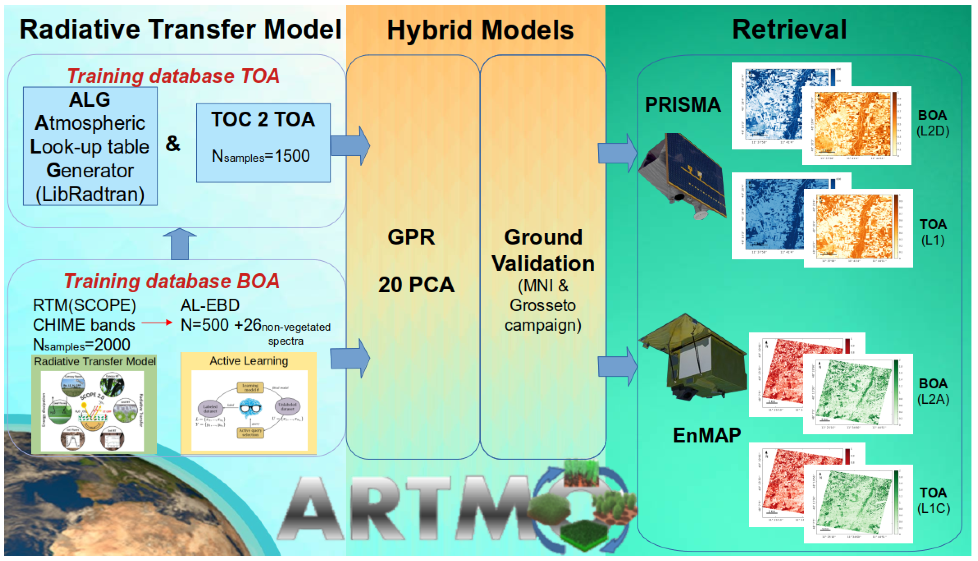
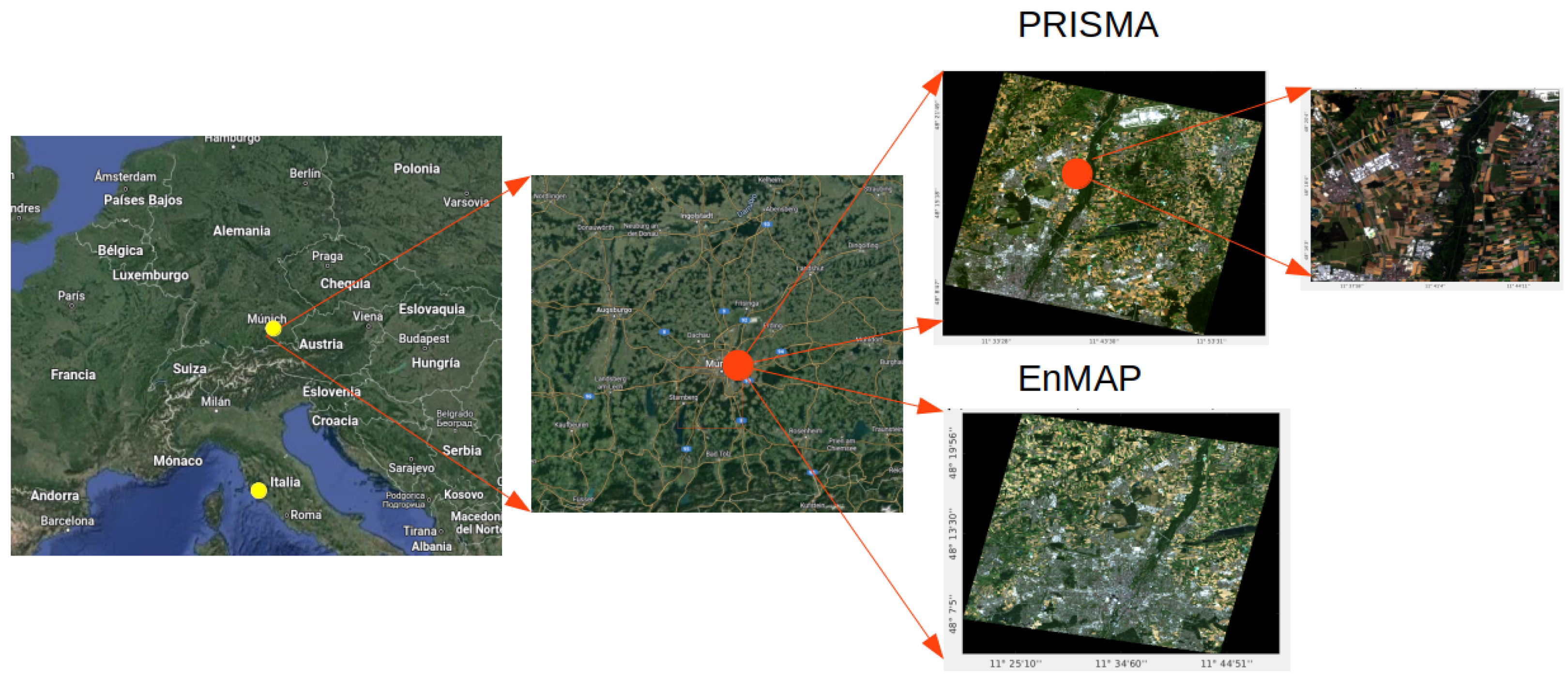
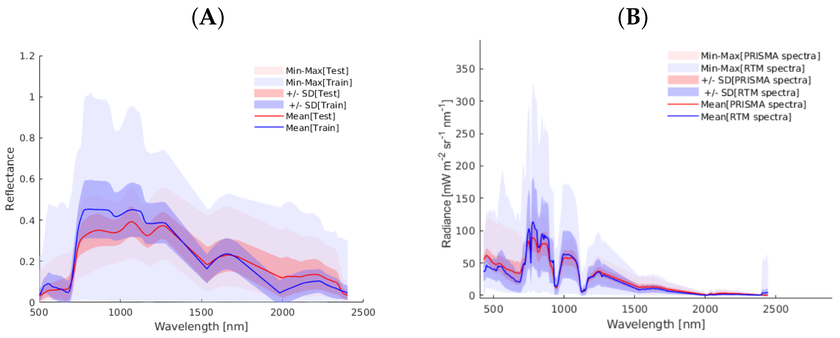
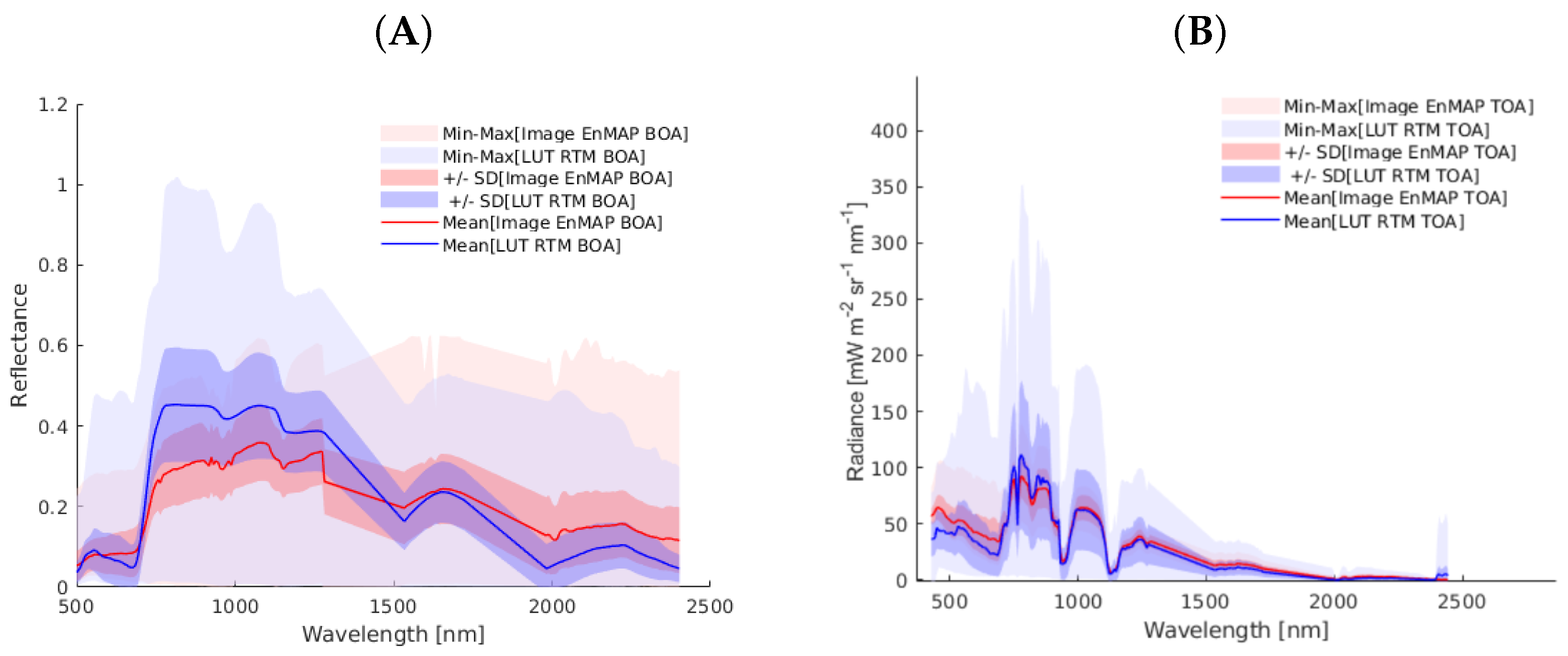
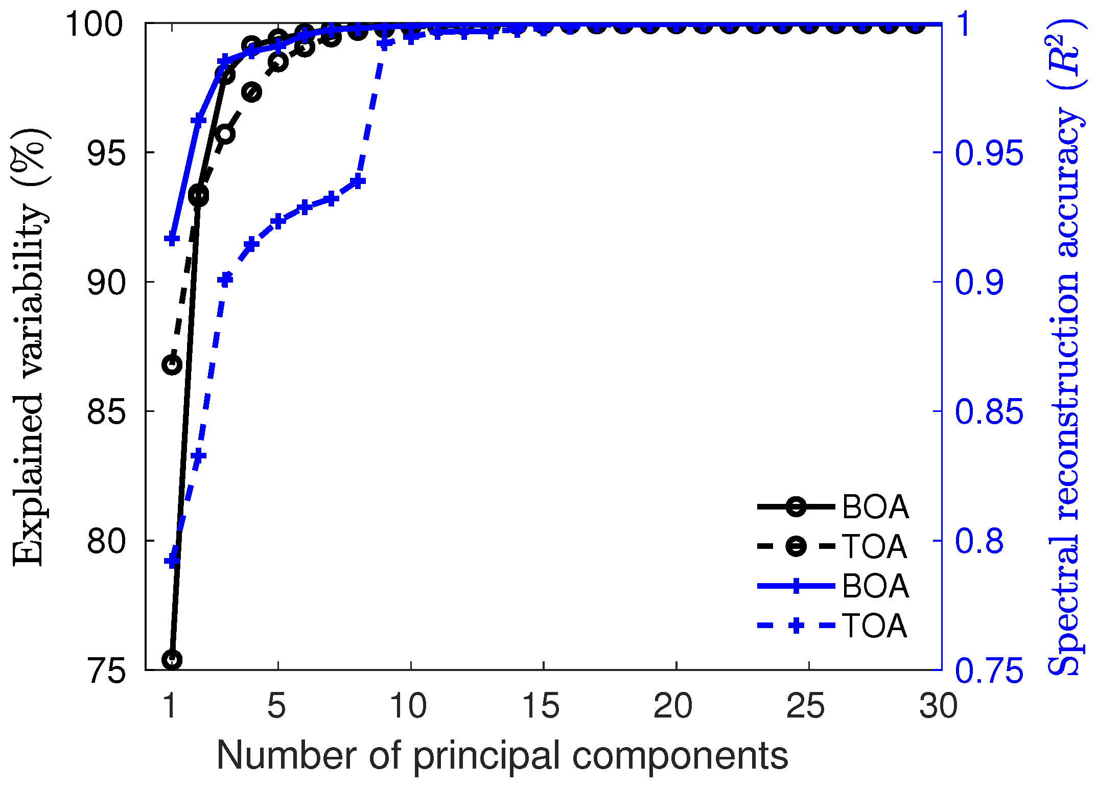
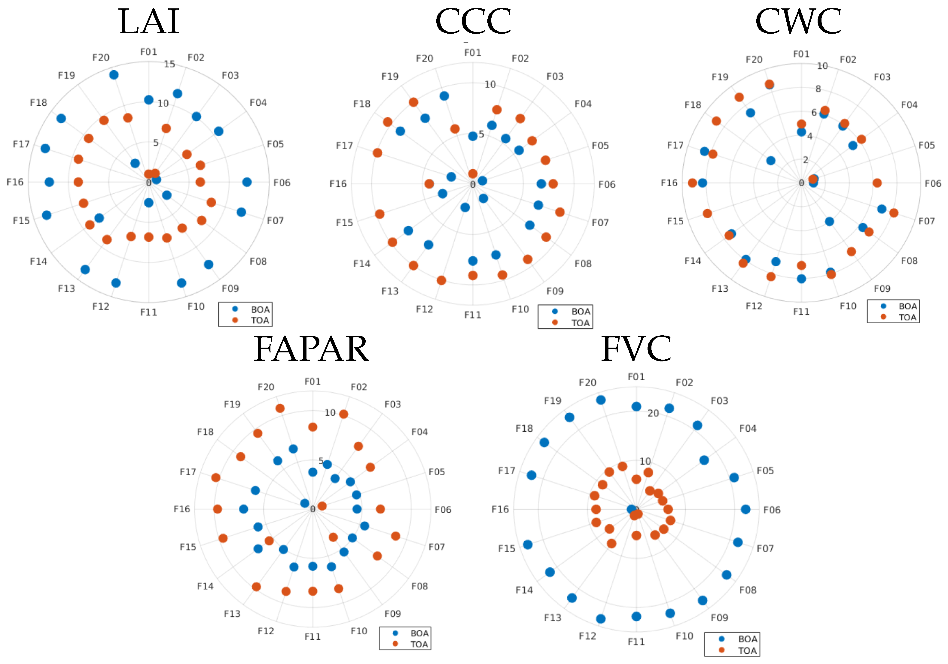
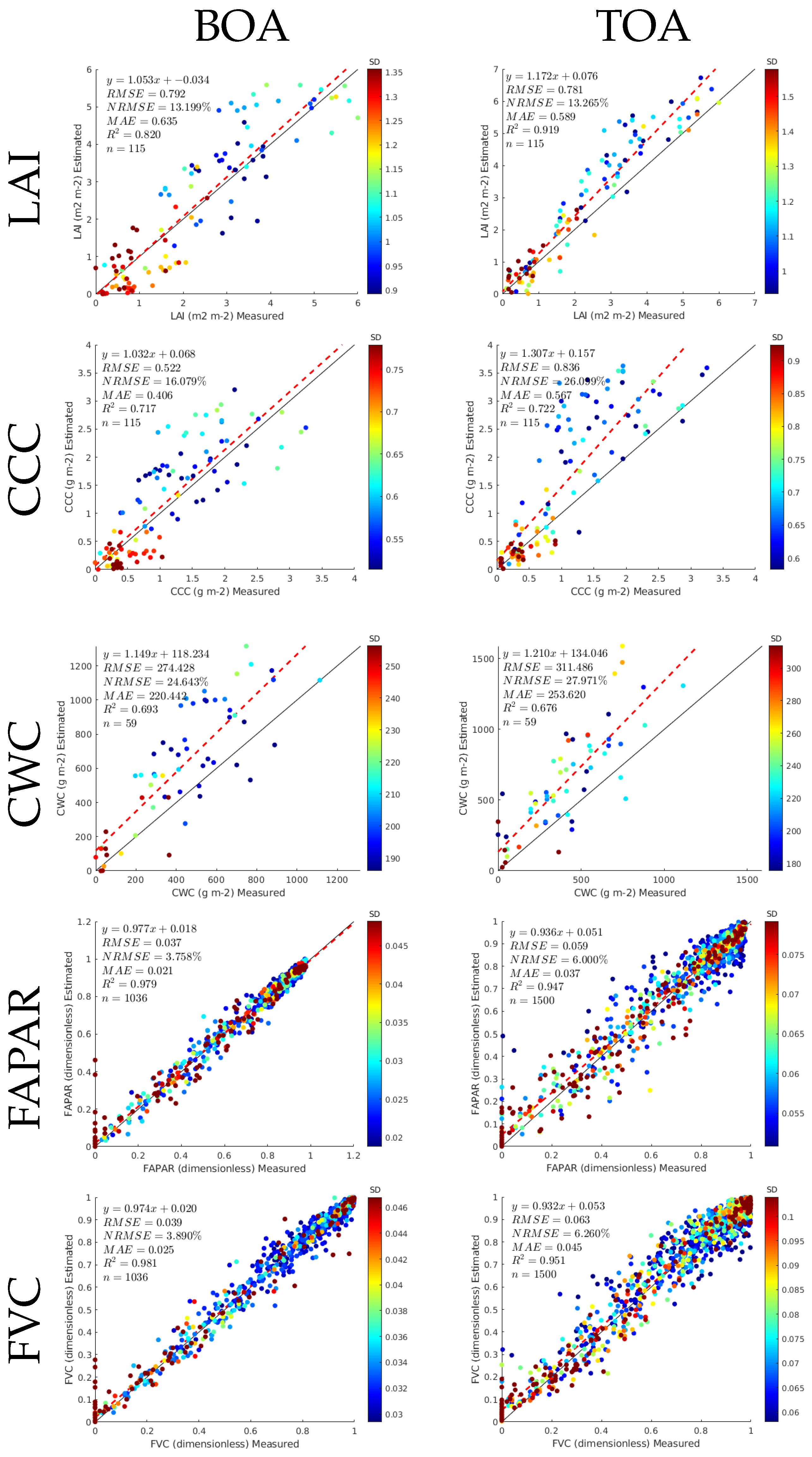

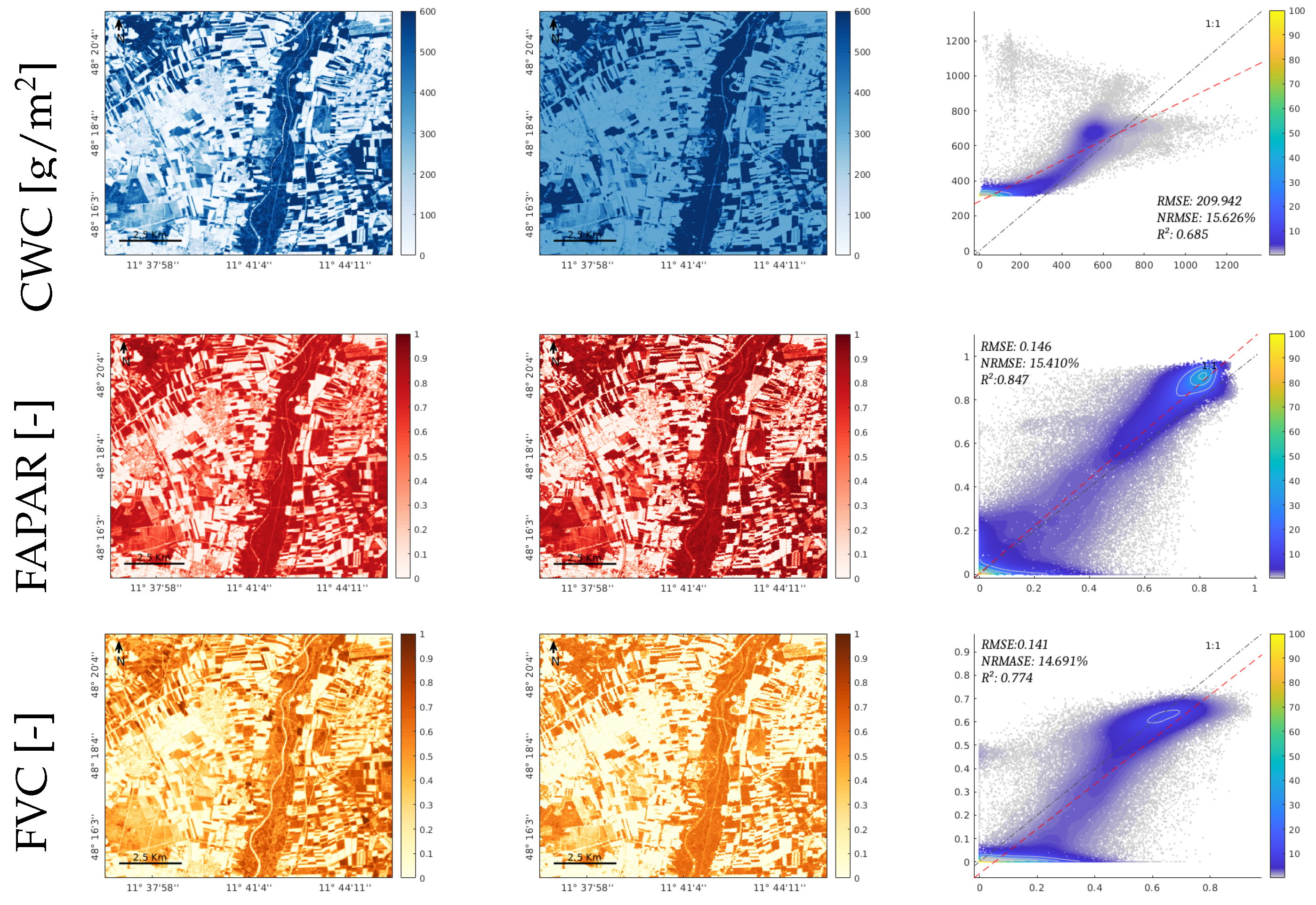
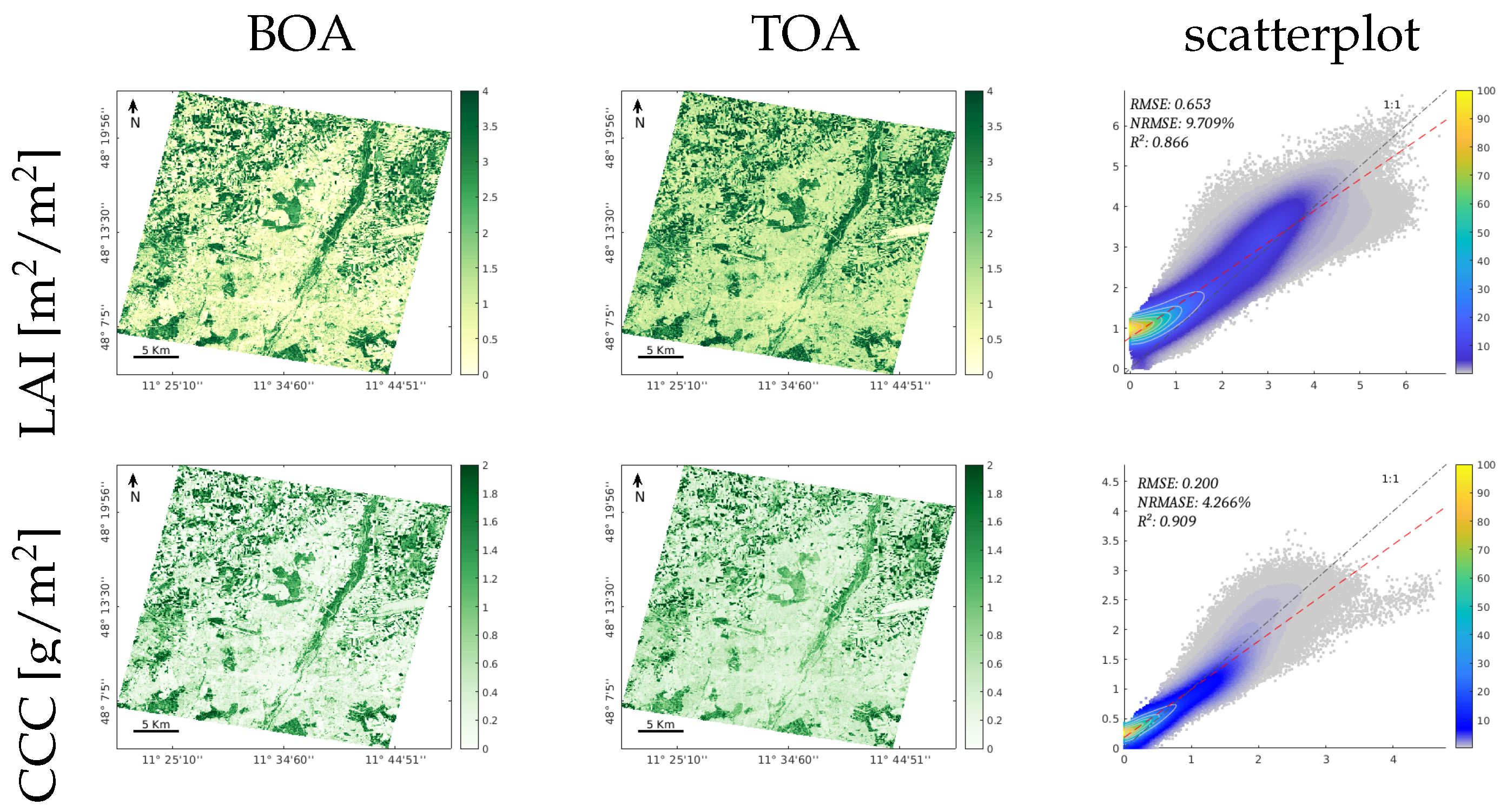
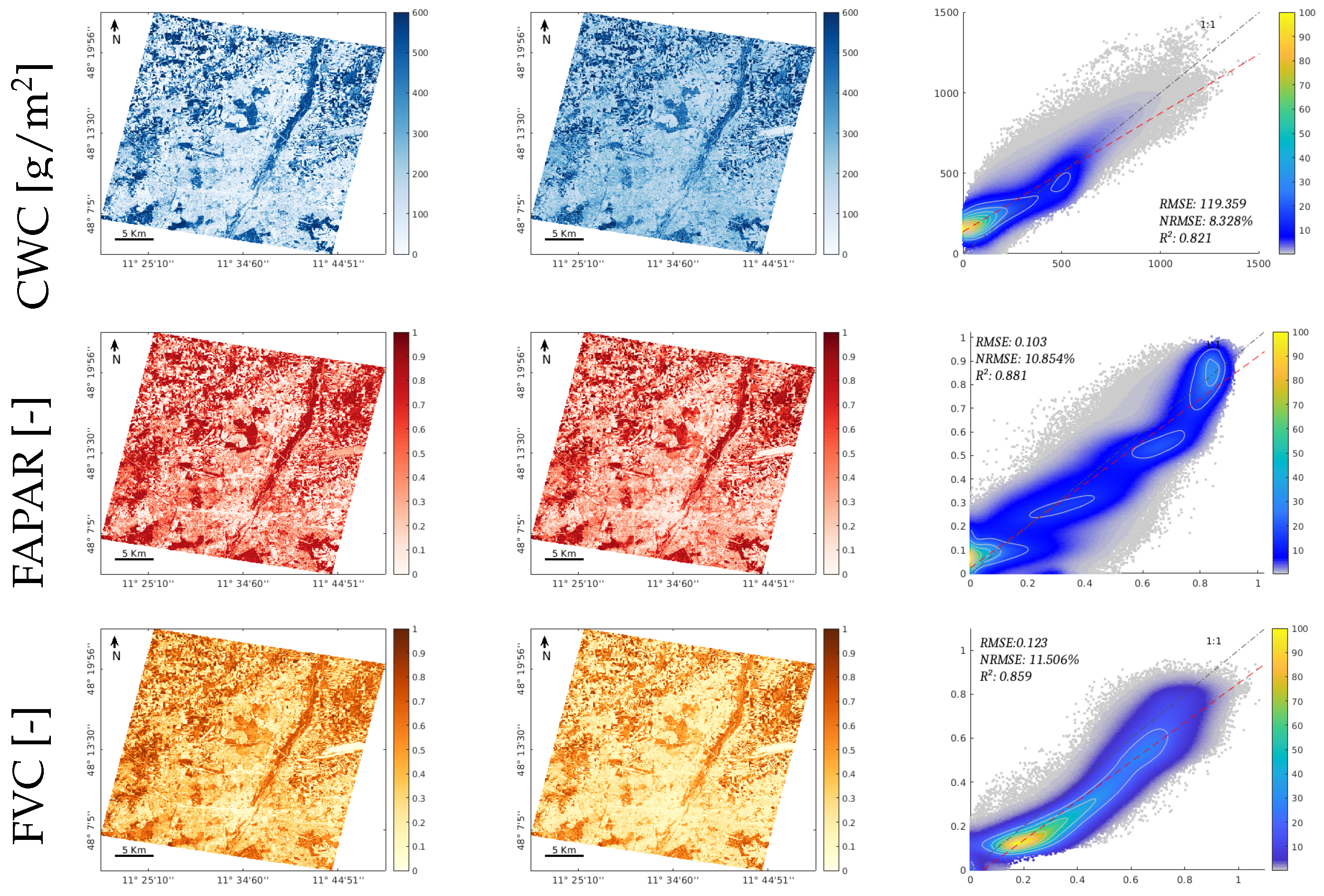
Disclaimer/Publisher’s Note: The statements, opinions and data contained in all publications are solely those of the individual author(s) and contributor(s) and not of MDPI and/or the editor(s). MDPI and/or the editor(s) disclaim responsibility for any injury to people or property resulting from any ideas, methods, instructions or products referred to in the content. |
© 2024 by the authors. Licensee MDPI, Basel, Switzerland. This article is an open access article distributed under the terms and conditions of the Creative Commons Attribution (CC BY) license (https://creativecommons.org/licenses/by/4.0/).