Satellite-Based Background Aerosol Optical Depth Determination via Global Statistical Analysis of Multiple Lognormal Distribution

Abstract

Determining background aerosol optical depth threshold value (BAOD) is critical to aerosol type identification and air pollution control. This study presents a statistical method to select the best BAOD threshold value using the VIIRS DB AOD products at 1 × 1 degree resolution from 2012 to 2019 as a major testbed. A series of multiple lognormal distributions with 1 to 5 peaks are firstly applied to fit the AOD histogram at each grid point, and the distribution with the highest correlation coefficient (R) gives preliminary estimations of BAOD, which is defined as either the intersection point of the first two normal distribution curves when having multiple peaks, or the midpoint between the peak AOD and the first AOD with non-zero probability when the mono peak is the best fit. Then, the lowest 1st to 100th percentile AOD distributions are compared with the preliminary BAOD distribution on a global scale. The final BAOD is obtained from the best cutoff percentile AOD distributions with the lowest bias compared with preliminary BAOD. Results show that the lowest 30th percentile AOD is the best estimation of BAOD for different AOD datasets and different seasons. Analysis of aerosol chemical information from MERRA-2 further supports this selection. Based on the BAOD, we updated the VIIRS aerosol type classification scheme, and the results show that the updated scheme is able to achieve reliable detection of aerosol type change in low aerosol loading conditions.

1. Introduction

Atmospheric aerosols play a key role in the earth-ocean-atmosphere system [1]. As a direct effect, they absorb and scatter the incoming short-wave solar radiation and the long-wave earth radiation; as an indirect effect, they modify the cloud formation processes by acting as the cloud condensation nuclei [2]. Aerosol particles can be emitted from various sources, such as the ocean, desert, wildfires, and urban/industrial emissions. Retrieving aerosol type information helps to characterize regional aerosol optical properties, track aerosol transport paths, and provide composition information for air quality research [3].

Background aerosol optical depth (BAOD) is a parameter characterizing the light extinction ability of local aerosol particles and represents the long-term stable level of aerosol concentrations from local emissions, rather than the long-range transport pollutants (i.e., dust storm), abrupt emission events (i.e., volcanic eruptions, wildfires), or unexpected aerosol accumulations due to adverse weather condition (i.e., haze). For a single site, BAOD could simply be regarded as a certain low level of AOD, but when applied to a large regional or global scale, BAOD should vary with locations; for example, BAOD in urban areas with anthropogenic emissions is supposed to be different from (generally higher than) BAOD at remote continent or grassland. Extracting BAOD from the total aerosol loading is important for us and model simulation to separate anthropogenic effects from natural variability and evaluate climate effects of specific aerosol types, e.g., urban/industrial, biomass burning, dust, etc. [4,5]. BAOD is also a key factor for some satellite retrieval algorithms performing atmospheric corrections of surface reflectance to remove aerosol contributions from satellite signals [6,7]. Thus, determining the BAOD threshold value is fundamental for both aerosol-climate effect assessment and satellite remote sensing correction.

Typical aerosols usually have certain AOD ranges. For example, background aerosols like clean continental and maritime aerosols often have an AOD value from 0 to 0.2, while anthropogenic and biomass-burning aerosols have much higher AOD, which ranges from 0.3 to 1.0, or even over 2 in some extremely polluted situations [8]. AOD is quite useful in identifying background aerosols, which are characterized by relatively low aerosol loading emitted from local sources [9,10]. Many previous studies have determined the BAOD threshold value when identifying aerosol types (e.g., urban industry, dust) from clean or background types. For example, Zhang, Kondragunta, Laszlo, Liu, Remer, Huang, Superczynski, and Ciren [6] used the lowest 5th percentile AOD as the estimate of the background AOD based on global AERONET observations; Xia, et al. [11] set the background level AOD₅₅₀ as less than 0.1 based on 40 ground-based observations across China; Petrenko, et al. [12] selected the peak histogram AOD as the background threshold for the month before the burning season; Chen, et al. [13] chose AOD₄₄₀ less than 0.2 as the background threshold over an urban area in Northeast China. These BAOD threshold values are generally determined by the researcher’s understanding of local emission and aerosol transport as well as their own experience and preference. There are also aerosol-type identification methods without the use of AOD [14,15], such as Angstrom Exponent and Single scattering albedo (AE-SSA) [16], fine mode fraction, and single scattering albedo (FMF-SSA) [17], and scattering Angstrom Exponent and absorbing Angstrom Exponent (SAE-AAE) [18]. However, it should be noted that the widely used aerosol properties, such as SSA and SAE from sun-photometer observations, are only available when AOD > 0.4. Therefore, these methods often miss the classification at AOD < 0.4 when ground-based sun-photometer products are used, and an AOD of 0.4 could be considered the hidden BAOD threshold value.

In addition to these ground-based studies, satellite sensors like VIIRS also provide global products with background aerosol information [19]. In the VIIRS aerosol classification algorithm, aerosols are divided into eight types, in which AOD less than 0.3 is identified as background type [3]. Different from ground-based observation, the selection of 0.3 as the BAOD threshold for VIIRS is more like a compromise to the limitation of the sensor and algorithm because the accuracy of AE is really limited when AOD is lower than 0.3. Aerosol type cannot be accurately identified, and thus, a ‘background’ type is used to represent these low-loading aerosol situations [20]. Zheng, Che, Xia, Wang, Yang, Chen, Wang, Zhao, Li, Zhang, Gui, Yang, Liang and Zhang [15] identified clean continent aerosols with AOD < 0.25 based on MODIS data. Chen, et al. [21] used an AOD threshold value of 0.2 to identify clean aerosols over China based on Himawari-8 observations, and the clean aerosol is identical to the background aerosol type. Whether for ground or satellite aerosol-type classification, the background AOD threshold value varies substantially from 0.1 to 0.3 and has not yet been properly defined. The classification of aerosol types, however, is rather sensitive to the selection of the BAOD threshold value [5,15,22]. Such a large variation in BAOD threshold value will cause uncertainty in the classification of aerosol types and decrease the comparability of similar studies [23,24,25]. Establishing a more reasonable and statistically based BAOD standard will help to unify the incoherence in aerosol-type studies, lower the level of difficulty in data comparisons, reduce the uncertainty in aerosol-type retrievals, and improve the quantification of the aerosol climate effects.

This study presents a reference map of global BAOD threshold values using a statistical method based on long-term satellite AOD observations from VIIRS, MODIS, and MISR. The statistical base of the BAOD determination involves multiple lognormal fitting processes for AOD histograms within each grid and an optimized process to search the best cutoff percentile of the lowest AOD on a global scale. With the help of the MERRA-2 dataset, we discussed the rationality of the BAOD from the chemical view, and we further discussed the implications of the BAOD threshold value for aerosol-type classification using VIIRS observations as an example.

2. Materials and Methods

2.1. Satellite AOD Data

VIIRS is a scanning radiometer onboard the Suomi National Polar-orbiting Partnership satellite launched in October 2011 [19]. It provides multi-spectral data twice per day, once during the daytime and once during the nighttime [26]. Aerosol properties are retrieved only during the daytime measurements at 1:30 P.M. local time. In this study, we choose VIIRS data as a testbed for our statistical method because of the following reasons: (1) VIIRS orbital swath is broader (by ~50%) than Moderate Resolution Imaging Spectroradiometer (MODIS), and it has no data gaps at equatorial regions and also twice or more sampling per day at the middle to high latitudes, which means VIIRS provides a broader spatiotemporal coverage of AOD measurement. (2) Since the aging of MODIS (especially Terra, launched in 1999) and Multi-angle imaging spectroradiometer (MISR, onboard) sensors, their data accuracy is getting unstable, and lots of efforts are needed to ensure the data is suitable for climate studies [3]. As a new generation sensor designed to continue the EOS-era data records, VIIRS will become the major sensor replacing MODIS soon. Thus, we choose the VIIRS DB AOD product as our major testbed. The VIIRS data used in this work is VIIRS V1 AOD from the Deep Blue Level 3 Daily aerosol data in the Level 1 Atmosphere (Archive Set 5110) collection (AERDB_D3_VIIRS_SNPP). The spatial resolution of the data is 1 × 1 degree, and the temporal coverage is from March 2012 to December 2019. Also, the latest MODIS C6.1 Level 3 Daily AOD product from Dark Target (DT), Deep Blue (DB), and their fusion (DTB) (MOD08_D3 for Terra and MYD08_D3 for Aqua) and MISR Version 23 Level 3 Global AOD product (MIL3DAEN) are also included to analyze the influence of spatial-temporal coverage of AOD on the determination of BAOD threshold value. VIIRS and MODIS data can be found at NASA’s Level-1 and Atmosphere Archive and Distribution System Distributed Active Archive Center (https://ladsweb.modaps.eosdis.nasa.gov/, accessed on 25 March 2024), and MISR data can be found at the Atmospheric Science Data Center (https://eosweb.larc.nasa.gov/project/misr/misr_table, accessed on 25 March 2024). The time ranges for MODIS and MISR AOD are from January 2012 to December 2019.

2.2. AERONET Data

Aerosol Robotic Network (AERONET) is a ground-based remote sensing network that provides long-term and continuous aerosol properties around the world [27]. The AERONET collaboration provides globally distributed observations of spectral AOD, inversion products, and precipitable water. These products are often used in aerosol-related research and satellite data validations [28]. The AERONET data are publicly accessible at the AERONET Team website at NASA Goddard Space Flight Center (http://aeronet.gsfc.nasa.gov/, accessed on 25 March 2024). In this work, Level 2.0 daily AODs at 440 nm and 670 nm in the AEROSOL OPTICAL DEPTH (V3)-SOLAR collection are used to obtain AOD₅₅₀ using an Angstrom Exponential relation. The interpolated AOD is regarded as the ground truth value to validate the VIIRS AOD.

2.3. MERRA-2 Aerosol Chemical Data

The Modern-Era Retrospective Analysis for Research and Applications, version 2 (MERRA-2), was developed by the NASA Global Modeling and Assimilation Office (GMAO) [29]. There are two primary objectives of developing MERRA-2: one is to assimilate data from NASA’s Earth Observation System (EOS) and demonstrate its usefulness for climate study, and the other is to improve the representation of the atmospheric hydrological cycle in reanalysis models compared to previous ones. MERRA-2 reanalysis data has a resolution of 0.625° longitude by 0.5° latitude on a global scale, and it provides hourly column mass density of black carbon (BC), organic carbon (OC), dust, SO₄, sea salt, SO₂, and Dimethyl sulfide (DMS) [30]. MERRA-2 data are available at MDISC, managed by the NASA Goddard Earth Sciences (GES) Data and Information Services Center (DISC) (https://disc.gsfc.nasa.gov/datasets?project=MERRA-2, accessed on 25 March 2024). Since this study focuses on background AOD over land, only column mass densities of BC, OC, dust, SO₄, and SS are taken into account. The time period of MERRA-2 data used in this study is between 2018 and 2019 (two years).

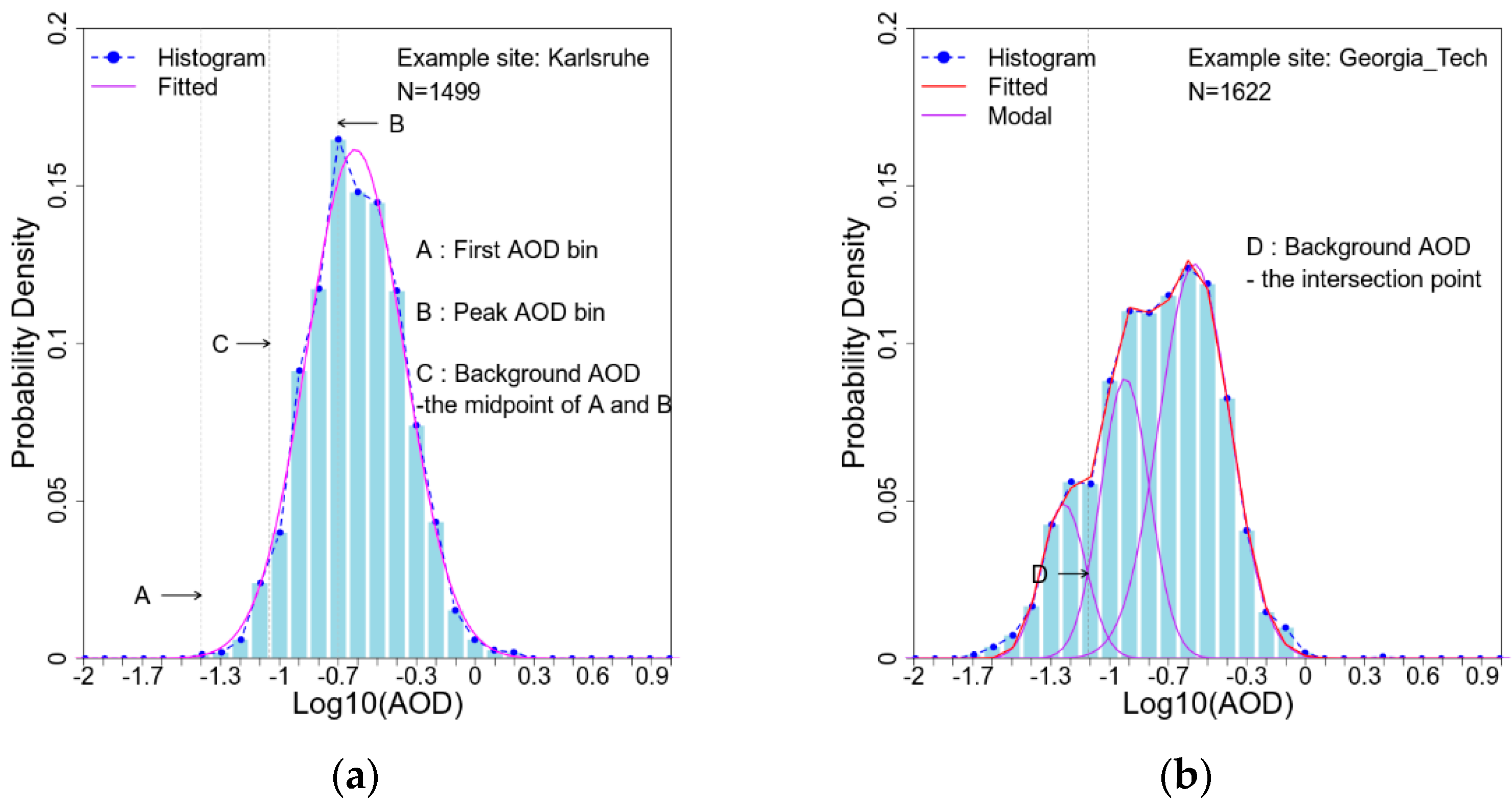
2.4. Multiple Lognormal Distribution Fitting for AOD Histogram

This study determines BAOD values by utilizing multiple lognormal fitting processes for AOD histograms within each grid. Multiple models in AOD histogram can be a representation of aerosol species [31,32]. The AOD histogram for each grid is created using a log10 AOD space ranging from −2 to 1 with an interval of 0.1 (a total of 31 bins with AOD ranging from 0.01 to 10). In each grid, five lognormal distributions with 1 to 5 modes are fitted to the histogram. $\mathrm{P}\left(\mathrm{l}\mathrm{o}\mathrm{g}\mathsf{\tau }\right)$ denotes the fitted AOD histogram for the five lognormal distributions. Function F is used to evaluate the fitting performance of the five lognormal distributions. The lognormal mode number with the lowest F value is considered the best estimation. Specifically, the target function is the square of the absolute bias between the AOD histogram and the fitted one.

$$P(\log \tau )={\displaystyle \sum _{i=1}^m\frac{P_i}{{\sigma }_i\sqrt{2\pi }}\times \exp (-\frac{\log ({\tau }^2/{\mu }_i^2)}{2{\sigma }_i^2})}$$

(1)

$$F={\displaystyle \sum _{j=1}^n{\left[P_{fit}(\log {\tau }_j)-P_{hist}(\log {\tau }_j)\right]}^2}$$

(2)

where τ represents AOD, m denotes the number of lognormal modes ranging from 1 to 5, $\mathrm{P}\left(\log \mathsf{\tau }\right)$ is the probability density of m lognormal with modal probability density P_i, geometric mean μ_i, and standard deviation ${\mathsf{\sigma }}_{\mathrm{i}}$, F is the target function, $\mathrm{j}$ represents the j-th AOD bin, ${\mathrm{P}}_{\mathrm{fit}}$ represents the fitted probability density function, and ${\mathrm{P}}_{\mathrm{hist}}$ is the reference probability density function from the AOD histogram.

The least squares method is used for fitting. The main idea of the least squares method is to minimize the sum of the squares of the errors (also known as residuals) of the true and predicted values by determining the unknown parameters (usually a matrix of parameters). The loss function F can be treated as a multivariate function, and F is a partial derivative of the parameters, respectively, so that the partial derivatives are equal to 0. Thus, a system of nonlinear equations is obtained, and then the iterative method is used to solve for the unknowns (i.e., P_i, μ_i, and σ_i).

$$\frac{\partial F}{\partial P_i}=\frac{\partial F}{\partial {\sigma }_i}=\frac{\partial F}{\partial {\mu }_i}=0$$

(3)

$$\min f(\mathbf{x})={\displaystyle \sum _{i=1}^n{\left[P_{hist,i}-P_{fit,i}\right]}^2}$$

(4)

$$F(x+dx)=F\left(x\right)+dx{F}^{\prime }\left(x\right)+O\left({\alpha }^2\right)\approx F\left(x\right)+dx{F}^{\prime }\left(x\right)$$

(5)

where x is the unknowns (i.e., P_i, μ_i, and σ_i), dx is the perturbation, and F′ represents the derivative.

An initial guess pool for each AOD histogram is constructed before fitting. In this pool, the highest point of the mono-mode, the turning points for the multi-modes (second, third, and later peak points), and the points where the slope changes significantly make up the initial guess of mode locations and their corresponding probability densities serve as the initial guess of mode heights. The initial standard deviations are 0.5, 0.45, 0.3, 0.35, and 0.3 for 1 to 5 modes, respectively. The boundary of each mode is set to be the same as $>0$, $-2<<1$, and $0.05<<1$. If any of the three parameters in each mode exceeds the boundaries, the fit is rejected. For example, if a negative P_i value is observed in a bimodal distribution, this fit is rejected, and we turn to fit the trimodal distribution. To avoid redundant modes, we calculate the specific value of each mode on the log10 AOD space. If less than two positive values are detected, this mode is deleted. For instance, if a trimodal fit is performed and the third mode generates only two positive values in the entire log10 AOD space, with all other values being zero, we delete the mode and degrade the trimodal distribution to a bimodal distribution. Sites with fewer than 60 observations are avoided during each fitting process because they are statistically insignificant and may cause unstable or unrealistic fitting results.

The best fit goes to the lognormal distribution with the lowest F values. The preliminary BAOD is either the intersection point of the first two normal distribution curves when having multiple modes, or the midpoint between the peak AOD and the first AOD with 1/10 peak probability density values when the mono normal distribution is the best fit (Figure 1).

2.5. Determination of the Best Cutoff Percentile for BAOD

Since the preliminary BAOD is obtained from statistical methods, the results will be inevitably influenced by factors such as the difference in the observation number in each grid and the data accuracy. Thus, the preliminary BAOD may not be smooth, and some outliers may appear. To avoid the outliers, we create 100 guesses with the lowest 1st to 100th AOD as reference BAODs and select the best cutoff percentile for the final BAOD threshold value. To determine the best estimation of BAOD, we have two target functions: an absolute bias (R) between the preliminary and guess BAOD and the other is a relative bias (Q).

$$R={\displaystyle \sum _{lon=-180}^{180}\sum _{lat=-90}^{90}{({\mathrm{BAOD}}_{lon,lat}^k-{\mathrm{BAOD}}_{lon,lat}^{pre})}^2},$$

(6)

$$Q={\displaystyle \sum _{lon=-180}^{180}\sum _{lat=-90}^{90}{(1-\frac{{\mathrm{BAOD}}_{lon,lat}^k}{{\mathrm{BAOD}}_{lon,lat}^{pre}})}^2},$$

(7)

where ${\mathrm{BAOD}}_{lon,lat}^k$ represents the AOD of the lowest kth percentile, and ${\mathrm{BAOD}}_{lon,lat}^{pre}$ is the preliminary BAOD; R and Q are the k-th absolute and relative bias, respectively. The best cutoff percentile is chosen as the percentile with the lowest R and Q, and the results based on VIIRS data are presented in Section 3.3.

2.6. IDW Interpolation

To evaluate the rationality of the reference BAOD obtained from VIIRS AOD using the methods described in Section 2.4 and Section 2.5, a ground-based BAOD map from global AERONET sites is obtained using an Inverse Distance Weight (IDW) interpolation [6]. The IDW interpolation is a deterministic method for multivariate interpolation with a known scattered set of points. The values at unknown points are calculated with a weighted average of the values available at the known points. A general form of finding an interpolated value y at a given point x based on samples ${\mathrm{y}}_{\mathrm{i} }=\mathrm{y}({\mathrm{x}}_{\mathrm{i}})$ for $\mathrm{i}=1,2,\dots ,\mathrm{N}$ using IDW is an interpolating function:

$$y(x)=\{\begin{array}{c}\frac{{\displaystyle \sum _{i=1}^N}{w}_i(x)y_i}{{\displaystyle \sum _{i=1}^N}{w}_i(x)}\hspace{1em},if\hspace{1em}d(x,x_i)\ne 0\\ y_i\hspace{1em},if\hspace{1em}d(x,x_i)=0\end{array},$$

(8)

where $w_i=1/d{(x,x_i)}^p$ is the IDW weighting function, x denotes an interpolated point, ${\mathrm{x}}_{\mathrm{i}}$ is an interpolating (known) point, d is the distance from the known point ${\mathrm{x}}_{\mathrm{i}}$ to the unknown point x, N is the total number of known points, and p is the power parameter [33]. Specifically, ${\mathrm{x}}_{\mathrm{i}}$ denotes the BAOD values from the i-th AERONET site using the same multiple lognormal fitting processes described in Section 2.4, and x denotes the same grid point as that in the VIIRS BAOD map.

3. Results

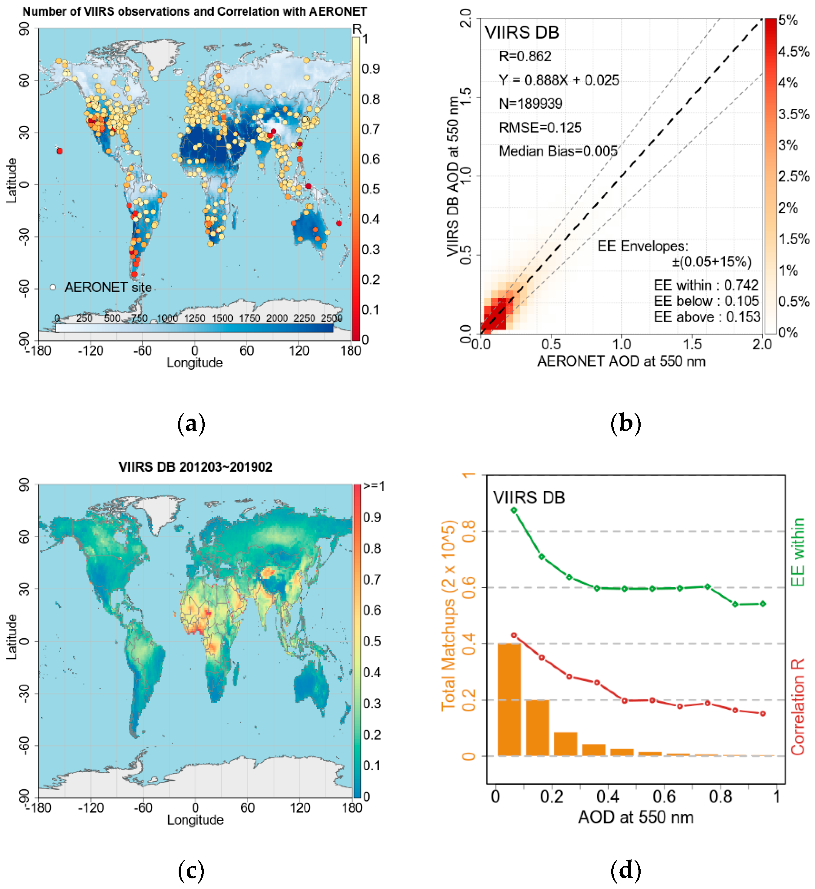
3.1. VIIRS DB AOD Comparison with AERONET AOD

The temporal coverage of the VIIRS DB AOD measurement is shown in Figure 2a. VIIRS DB AOD product has a high temporal coverage between 10 N and 50 N and between −10 N and −50 N, while a much lower temporal coverage is observed between the two belts. Such a temporal coverage difference is probably due to the high occurrence of clouds near the equator [34]. The scattering circles in Figure 2a illustrate the 697 AERONET sites used in evaluating the VIIRS DB AOD products. The vertical color bar illustrates the magnitude of the correlation between AERONET and VIIRS DB AOD, and the horizontal color bar indicates the VIIRS DB AOD observation frequency. Since AERONET provides a point observation with a sampling frequency of 5–15 min while satellite provides a regional snapshot at a single time, a spatiotemporal matchup scheme is applied. To be specific, AERONET data is firstly averaged within a time window of ±30 min from the satellite overpass, and then a spatial average is conducted if more than one AERONET observation is available in the 1° × 1° grid cell.

Figure 2b shows the overall statistics based on 189,939 common observations from paired AERONET and VIIRS observations. VIIRS DB AOD generally performs well in most AERONET sites and has an overall correlation of 0.862 with AERONET AOD, and 74.2% of VIIRS DB AODs fell in the estimated error (EE) envelopes of $\pm (0.05+15\%)$. The VIIRS DB data set was previously validated by Sayer et al. [35] on an instantaneous basis. Compared with the results from Sayer et al. [35], a similar RMSE (0.125) and median bias (0.005) values were obtained. Their correlation R (0.82) is slightly higher, while the Estimated Error envelope (EE) within the ratio (0.80) is a little bit lower. We also observe a regional dependency on the correlation, which is in agreement with the results from Sayer et al. [35]. The correlation coefficients tend to be less than 0.4 over low AOD areas like southwest Africa and Australia, as well as highly elevated terrain such as the Rocky Mountains and the Tibetan Plateau in western China, while they are close to 1 over other regions with high aerosol loading or low elevated terrain [3]. Figure 2d shows the VIIRS DB AOD performance over the low AOD regime. High EEs with a ratio >60% are observed for low AOD bins (0–0.3), which indicates that most of the observations fall into the EE envelope of ±(0.05 + 15%).

A high correlation of 0.862 between VIIRS and AERONET AOD indicates that VIIRS AOD can accurately represent the daily variation of aerosol loadings globally. The low fitting intercept of 0.025 suggests that VIIRS generally overestimates AOD by 0.025, which is higher than the AERONET uncertainty of 0.01 but still accurate for satellite observations. However, it is important to note that such overestimation on VIIRS AOD would be passed to BAOD threshold values. AOD observations fall within the expected error, which means a maximum overestimation or underestimation of around 0.1 when AERONET AOD is lower than 0.3. Low R or EE ratios are observed in southwest Africa and Australia, as well as highly elevated terrain such as the Rocky Mountains and the Tibetan Plateau in western China. This can lead to an imprecise estimation of the absolute BAOD threshold value, and BAOD from satellite observations in these regions needs further examination before usage.

3.2. Global AOD Distribution

Figure 3 shows the map of VIIRS DB AOD at different lowest percentiles. The lowest 50th percentile (the median), 25th and 75th percentile (50% of the data), 16th and 83rd percentile (one-standard deviation, 68% of the data), and 3rd and 97th percentile (two-standard deviation, 95%) of AOD are selected to show the global AOD characteristics. The AOD map shown in Figure 3a with the lowest 3rd percentile could be regarded as the cleanest aerosol condition for different regions. The lowest 3rd percentile AOD in most parts of the world is lower than 0.1; however, a relatively high AOD above 0.2 is observed in the northern part of South America, North Africa, and India, indicating a high aerosol loading base. With the increase of percentile, a relatively fast increase of AOD is observed in the Middle West Africa, Middle East, India, and East Asia (Figure 3a–e), which indicates these regions are the major aerosol sources around the world. From Figure 3f, 83% of AOD in most parts of North and South America, South Africa, Europe, Australia, and North Asia are below 0.3, which means an overall clean aerosol condition over these regions. However, from the lowest 97th percentile AOD map (Figure 3g), extremely high AOD events (AOD > 1) appear in some of these clean regions. The extreme AODs found in the northern part of North America and the tropical region of South America are mostly from biomass-burning smoke [3]. Those extreme AODs observed in East Asia are partly due to the heavy anthropogenic emissions and partly due to transported dust from the desert region and occasionally biomass-burning smoke from Siberia and Southeast Asia [36]. Also, 97% of AODs are found always below 0.3 over the southwest part of North and South America, the southern part of South Africa, North Europe, and the Non-desert region of Middle Asia (e.g., Tibetan Plateau) and West Australia, indicating a year-round clean aerosol condition.

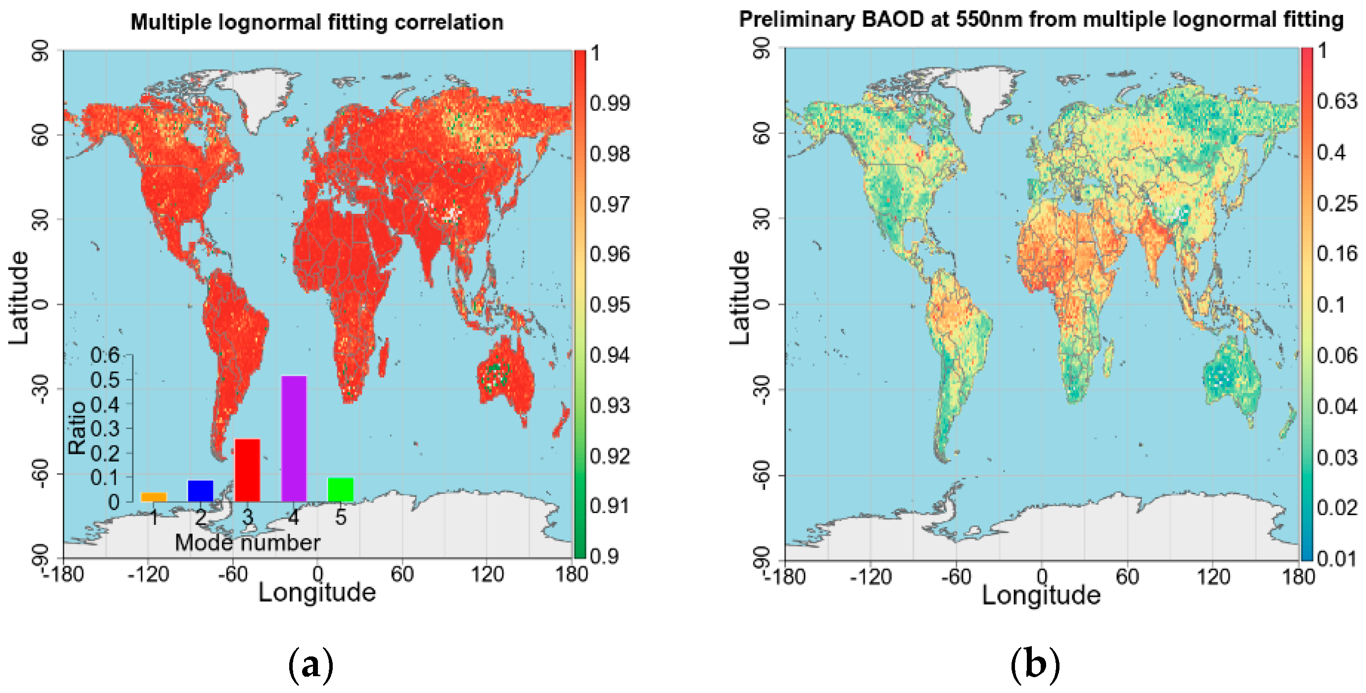
3.3. Preliminary BAOD from Multiple Lognormal Fitting

Figure 4a shows the global multiple lognormal fitting correlation map. Most parts of the world have a very high fitting correlation of over 0.98. Although relatively low fitting correlations are observed over the high latitude northern hemisphere (50 N–80 N), the Tibetan Plateau, and Midwest Australia, it does not hinder the determination of BAOD threshold over these regions, and a generally ‘smooth’ BAOD map is finally obtained despite some abrupt points with abnormal BAOD values. The quadruple and triple lognormal modes are found to appear most frequently around the world and their combined fraction is around 80%. This high frequency of occurrence of multiple AOD modes indicates that aerosol types tend to vary among three or four kinds in most parts of the world [37].

The preliminary BAOD from multiple lognormal fitting is shown in Figure 4b. A distinct high BAOD is found over the Indo-Gangetic Plain, Arabian Peninsula, and North and Mid Africa since the annual mean AOD over these regions is generally over 0.4. Southeast Asia also has a relatively high annual mean AOD, but the preliminary BAOD there is much lower than in areas like the Indo-Gangetic Plain and the Arabian Peninsula. Such difference is due to the fact that aerosol loading over Southeast Asia varies in a wide range, and a number of AOD measurements fall in low AOD bins; thus, the corresponding AOD histogram has a potential mode in low AOD bins [38]. While in high BAOD regions like the Indo-Gangetic Plain and the northern part of South America, most AOD observations fall in relatively high AOD bins, leading to the AOD histogram moving towards the high AOD end. High BAOD values are also found in the eastern part of North America, for these areas have relatively large industrial emissions [4].

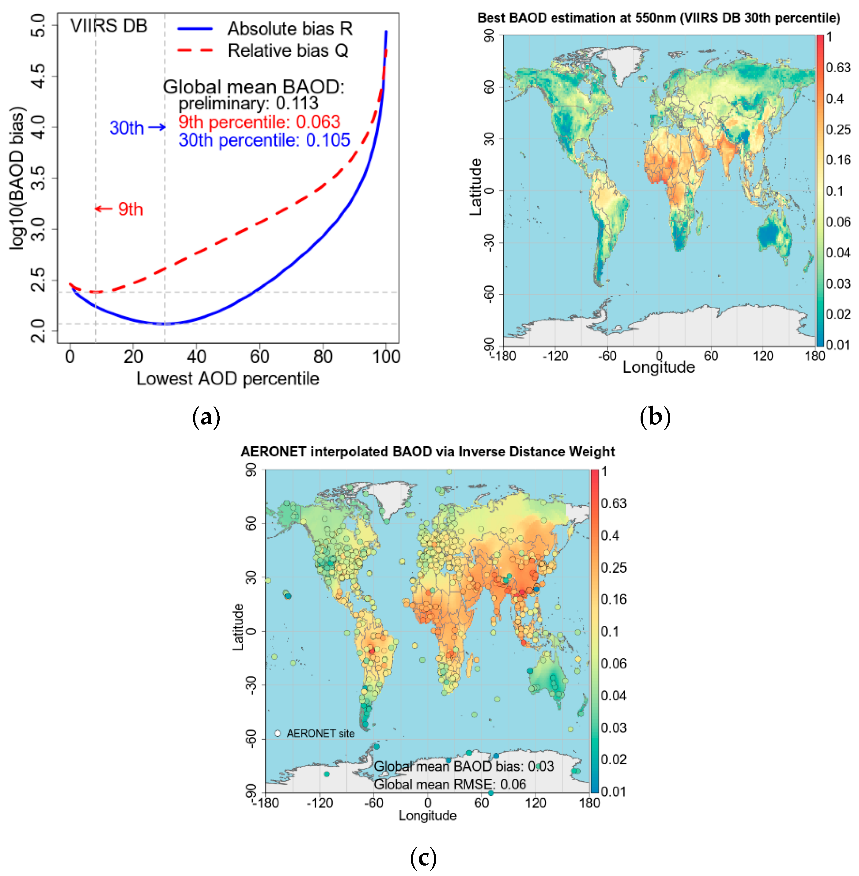
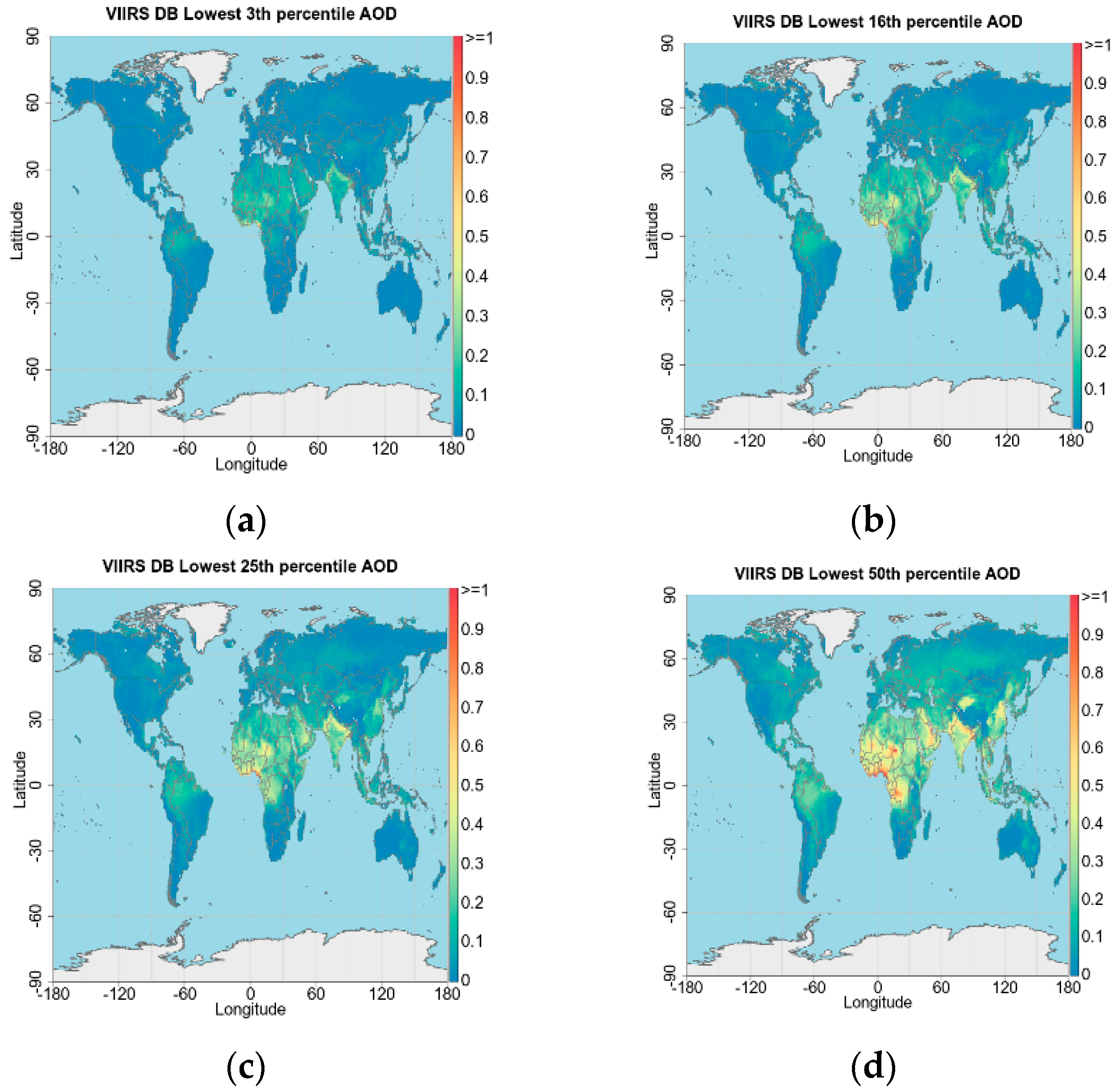
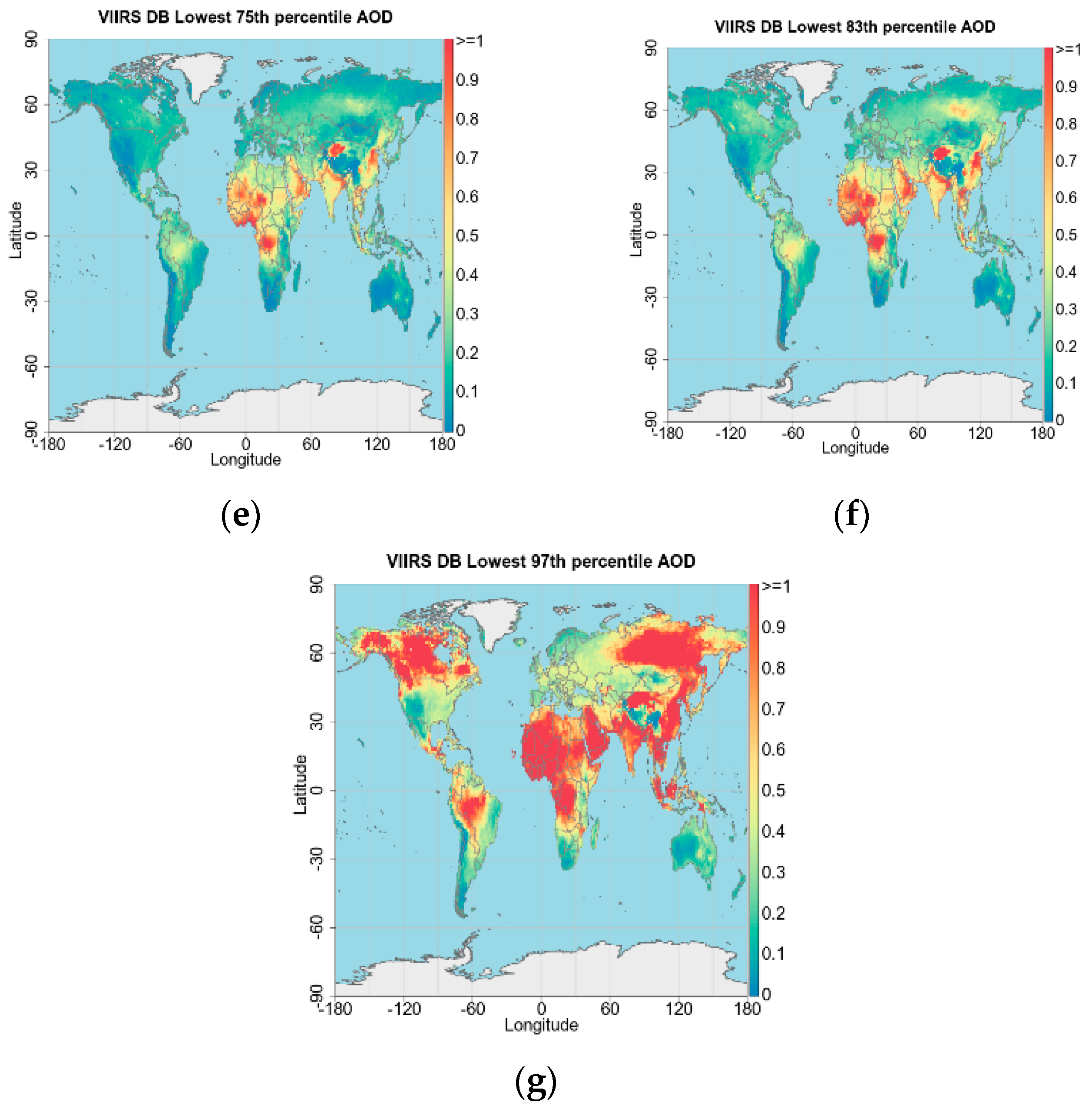
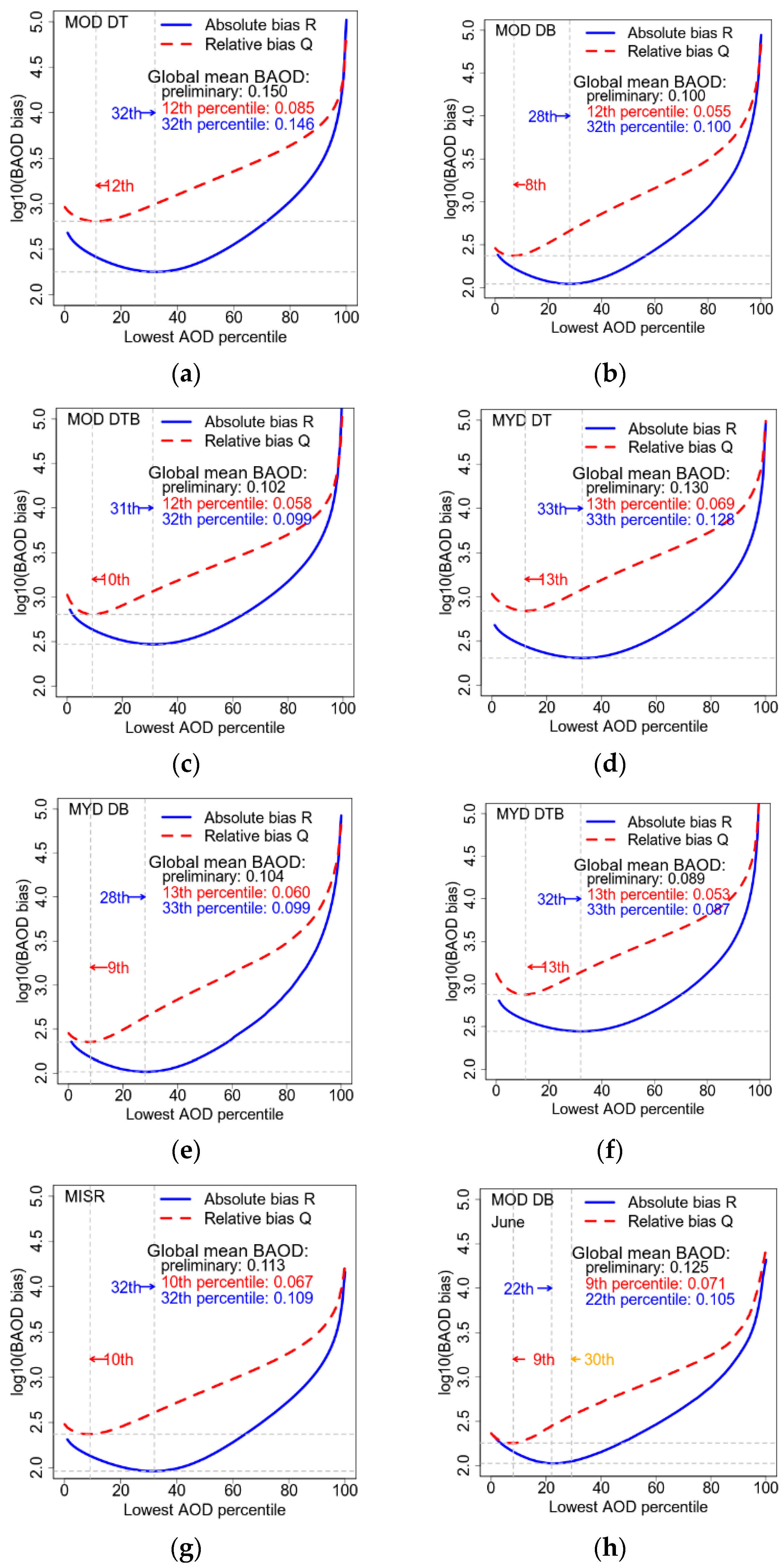
3.4. Best Cutoff Percentile of the Lowest AOD for Background Aerosol

Figure 5a shows the variations of BAOD bias (R and Q) with an increasing percentile of the lowest AOD. The lowest R and Q appear in the 9th and 30th percentile, respectively. Considering that the global mean BAOD from preliminary multiple lognormal fitting is 0.113, we select the 30th percentile of the lowest AOD as the best estimation of BAOD because its global mean (0.105) is very close to the preliminary mean BAOD of 0.113, while the 9th percentile is only about half (0.063). The final BAOD map (Figure 4b) shows similar patterns to those of the preliminary BAOD. North and Mid Africa, the Arabian Peninsula, North and Mid Africa, and the northern part of South America are still characterized by high BAOD threshold values. The eastern part of America has a slightly higher BAOD than the western part. Compared with Figure 4b, wider coverage of BAOD over 0.1 is observed over Europe and West Asia, and a distinct increase of BAOD from 0.1 to 0.4 is found in Southeast Asia. Such an increase is generally acceptable for the background aerosol loading because the annual mean AOD (especially in Southeast Asia, Figure 4b) is still much larger (nearly twice) than the lowest 30th percentile AOD.

To evaluate the rationality of the BAOD map in Figure 5b, the lowest 30th percentile of AERONET AOD is selected as AERONET BAOD value, and then the IDW interpolation method is applied to get a ground-based BAOD map. Here, the distance is set as 25 degrees, and the power parameter is set as 2 in the IDW interpolation. Figure 5c shows the ground-based interpolated BAOD map. We then calculate the global mean bias and RMSE between the lowest 30th percentile of VIIRS AOD and the IDW interpolated AOD from AERONET. The global mean BAOD bias and RMSE are 0.03 and 0.06, respectively. Similarly, high BAOD pools are observed over South America, North Africa, and North Asia, while low BAOD pools are over North America, Europe, and Australia. The interpolated AERONET BAOD map generally agrees well with the VIIRS BAOD map, indicating the rationality of the reference BAOD in Figure 4b. The differences between VIIRS BAOD and the BAOD obtained from AERONET mainly come from two aspects. One is that the interpolation process itself generates bias. Since the number of ground-based sites is limited, most regions are short of reliable observations. Since aerosols are of high spatiotemporal variation, the interpolated one may not be able to fully describe the variation of spatial aerosol conditions compared to satellite observations. The other is that, as a statistical method, the multiple lognormal fitting results may vary due to different inputs. Although high consistency between VIIRS and AERONET AOD is observed, a lot of observations outside the EE envelope (Figure 2b) will lead to changes in BAOD values and even outliers.

4. Discussion

4.1. Variation of BAOD to Different Satellite Datasets and Seasons

Due to the inconsistency of spatiotemporal coverage, systematic bias, and retrieval algorithm between different sensors, the best estimation of the BAOD threshold value may vary with different AOD products. To assess how the reference BAOD could vary with different satellite AOD inputs, we apply the same BAOD determination process to MISR and Terra- and Aqua-MODIS datasets. Figure 6a–g shows the overall fitting results from Terra-MODIS, Aqua-MODIS, and MISR AOD inputs. Similar to VIIRS, the best estimation of BAOD threshold value for MISR, Terra-MODIS, and Aqua-MODIS is selected between the 28th and 33rd percentile of their lowest AOD. Since the first derivatives of the absolute bias R are all around 0 in the vicinity of their best-fitting percentile, the difference is negligible between the 30th and 28th/33rd percentile of the lowest AOD being the best BAOD. Thus, the reference BAOD obtained from the current study varies little with different satellite AOD products, and the use of the 30th percentile of the lowest AOD as background AOD threshold value should be reasonable for various satellite sensors.

Aerosol loading and type usually vary with seasons, and such a seasonal variation may also have an impact on the determination of the best BAOD threshold value. Following the same data processing, the monthly mean BAOD threshold value from different sensors is shown in

Table 1. Seasonal summary of the best cutoff percentile of the lowest AOD for background aerosol for different AOD products. The seasonal MISR results are not available due to its limited input number (>60).

Dataset	Year 2012–2019	Month
		January	February	March	April	May	June	July	August	September	October	November	December	Average
VIIRS DB	30%	33%	32%	29%	27%	27%	27%	28%	28%	27%	32%	33%	31%	29.5%
MOD DB	28%	31%	27%	26%	24%	26%	22%	25%	25%	24%	25%	29%	31%	26.3%
MOD DT	32%	31%	28%	27%	28%	30%	27%	27%	27%	30%	28%	32%	31%	28.8%
MOD DTB	31%	27%	27%	27%	26%	27%	25%	26%	27%	38%	27%	28%	28%	26.9%
MYD DB	28%	30%	30%	28%	29%	27%	27%	30%	28%	30%	28%	29%	32%	28.9%
MYD DT	33%	30%	28%	29%	31%	29%	29%	28%	29%	32%	32%	32%	33%	30.2%
MYD DTB	32%	29%	28%	28%	29%	30%	29%	29%	29%	30%	28%	28%	29%	28.8%
MISR	32%	-	-	-	-	-	-	-	-	-	-	-	-	-
Average	30.8%	30.1%	28.6%	27.7%	27.7%	28.0%	26.6%	27.6%	27.6%	28.7%	28.6%	30.0%	30.7%	28.5%

. Due to the least data limitation (N > 60), the seasonal BAOD threshold value from MISR is not available here. In general, the monthly average best percentile is selected between 26.6 and 30.7. The best percentile shows an insignificant seasonal variation, which tends to be low in June and July while high in January and December. The largest difference to the reference 30th percentile is observed from the Terra-MODIS DB product, where the 22nd percentile in June is found to be the best estimation. Figure 6h shows the corresponding bias curve, and the use of the 30th percentile is acceptable because the difference in log bias between the 30th and 22nd percentiles is not very large. Therefore, the use of the 30th percentile of the lowest AOD as the background AOD threshold value is also reasonable for different months. It should be noted that although the BAOD threshold value is the 30th percentile, the monthly mean AOD will vary with seasons, and consequently, the reference BAOD value also has a seasonal variation.

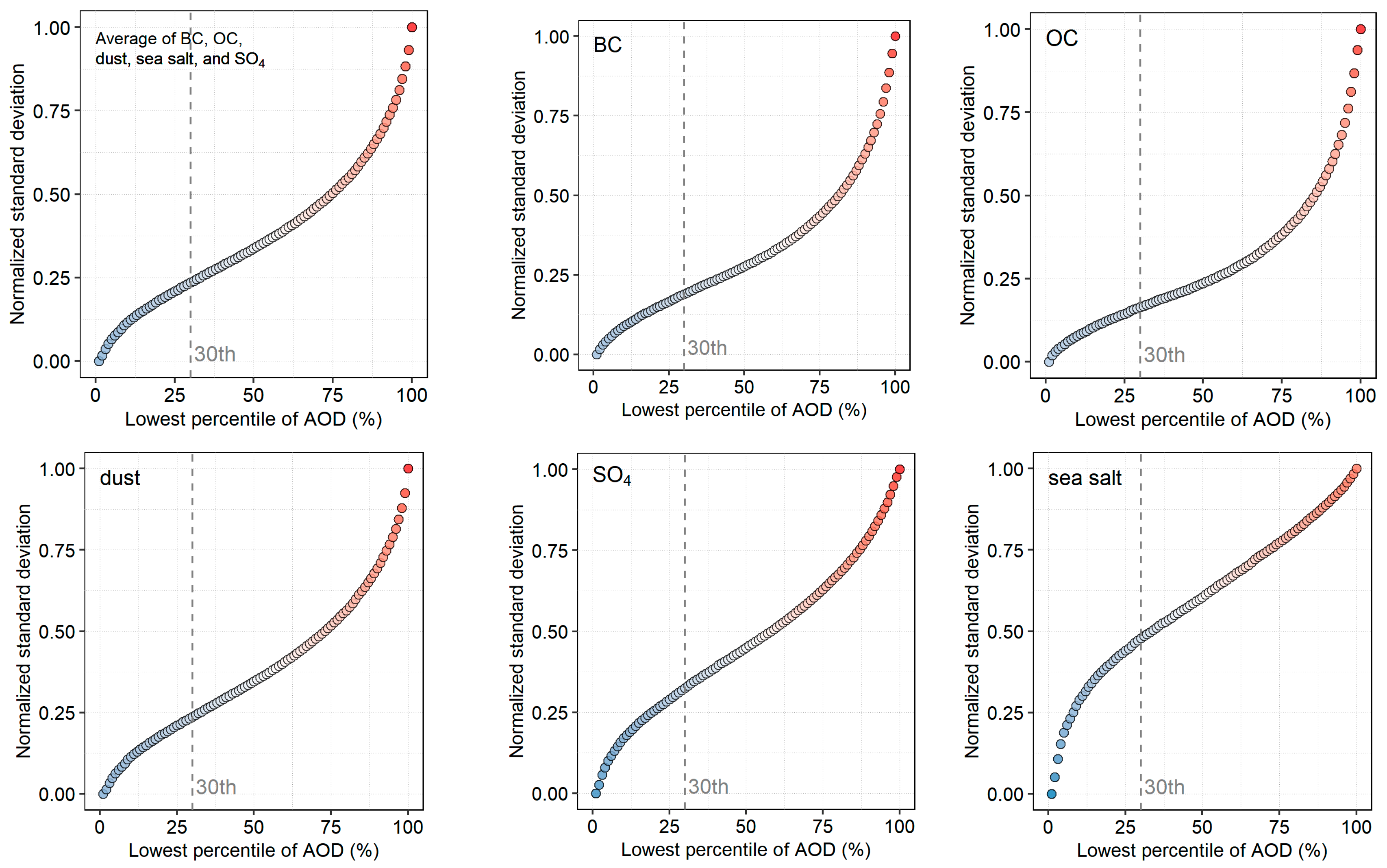
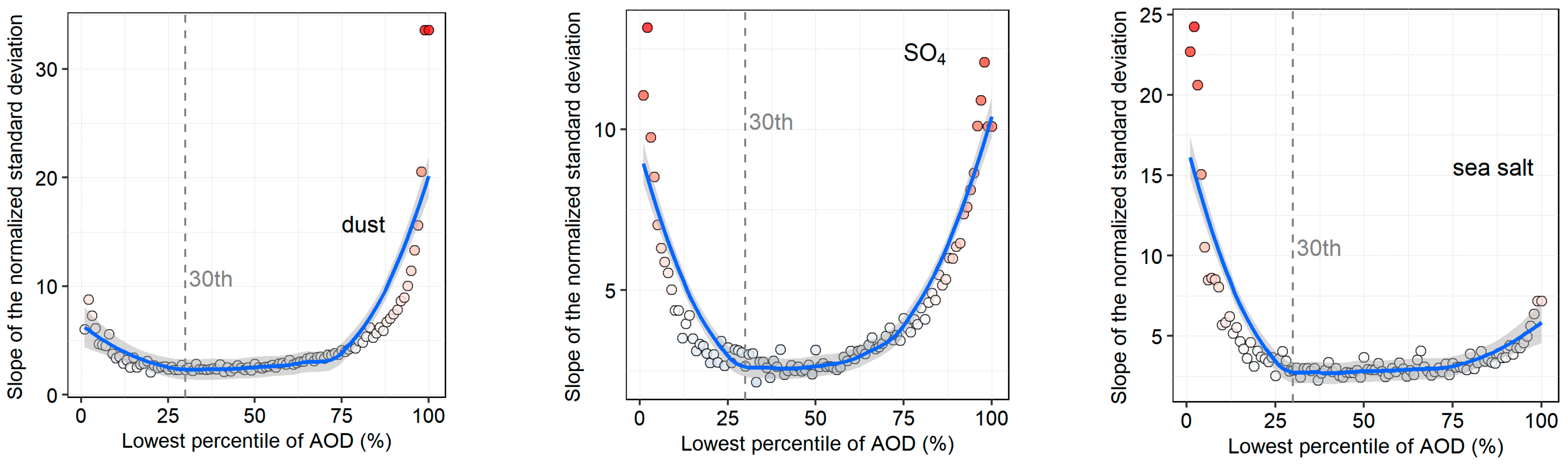
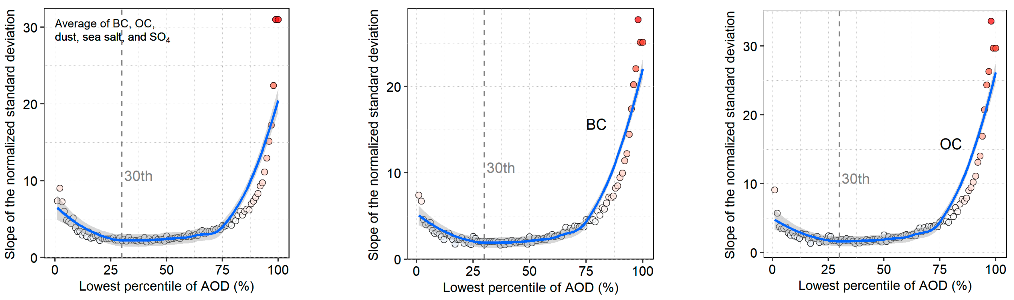
4.2. BAOD Determination from an Aerosol Chemical Perspective

Although we have determined that the 30th percentile of the lowest AOD is the best background AOD threshold through a statistical approach, it is preferred to validate this from a different perspective, such as a chemical view, to prove its rationality. Typical aerosol particles have specific chemical components [5,13], and therefore, the variation of aerosol types could be reflected by the variation of their chemical components [29]. The rationality of the BAOD threshold value is illustrated using the co-located aerosol chemical information from MERRA-2. A spatiotemporal matchup scheme is applied to ensure accurate validation. This is because VIIRS provides a regional snapshot at a single time, and the resolutions of MERRA-2 and VIIRS AOD are different. Specifically, hourly MERRA-2 data are first selected within a time window of ±30 min from the satellite overpass. Then, they are re-scaled at a resolution of 1° × 1°.

The global average variation of the normalized standard deviation of column aerosol mass density with the lowest percentile of AOD over land is shown in Figure 7. The increase of the lowest AOD percentile leads to an increase in the normalized standard deviation, indicating a corresponding increase in the degree of chemical component change. When AOD is located in the lowest 30th percentile, aerosol loading is relatively light, and there is little variation in chemical components (as indicated by a low standard deviation of both the average and each chemical).

Figure 8 shows a decreasing trend in slope variation of normalized standard deviation from 0 to the 30th lowest percentile AOD, followed by a stable slope variation from the 30th to around the 75th lowest percentile AOD. This indicates that the chemical component variations are gradually becoming more prominent before the 30th lowest percentile AOD, but they still remain at a low level of change, as indicated by the low standard deviation. After the 30th lowest percentile AOD, a relatively stable rate of change in chemical components is observed, indicating a gradual and significant shift in aerosol type as AOD increases (with a high standard deviation). Thus, from a chemical perspective, the aerosol type is generally stable when the AOD is low but becomes increasingly unstable as the AOD increases. The breaking point of the changing rate of the standard deviation occurs at the 30th lowest percentile AOD, which separates these two aerosol conditions.

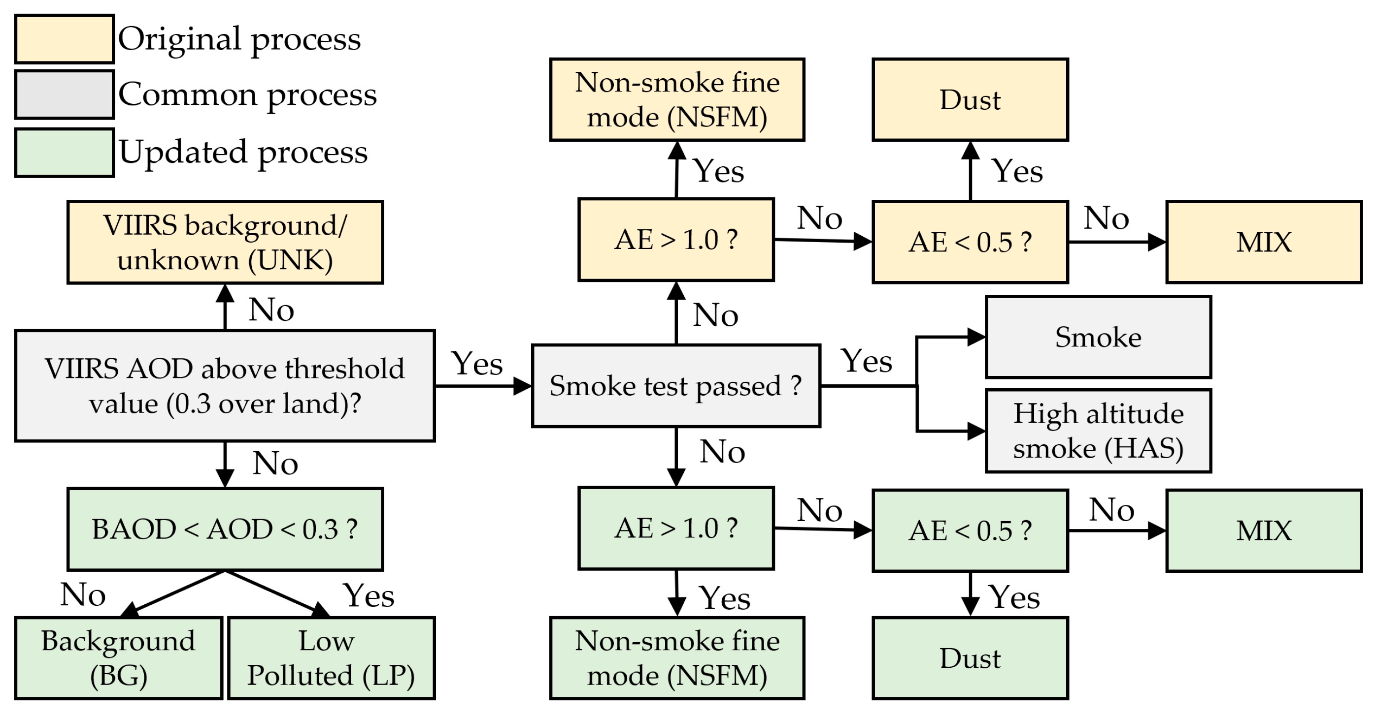
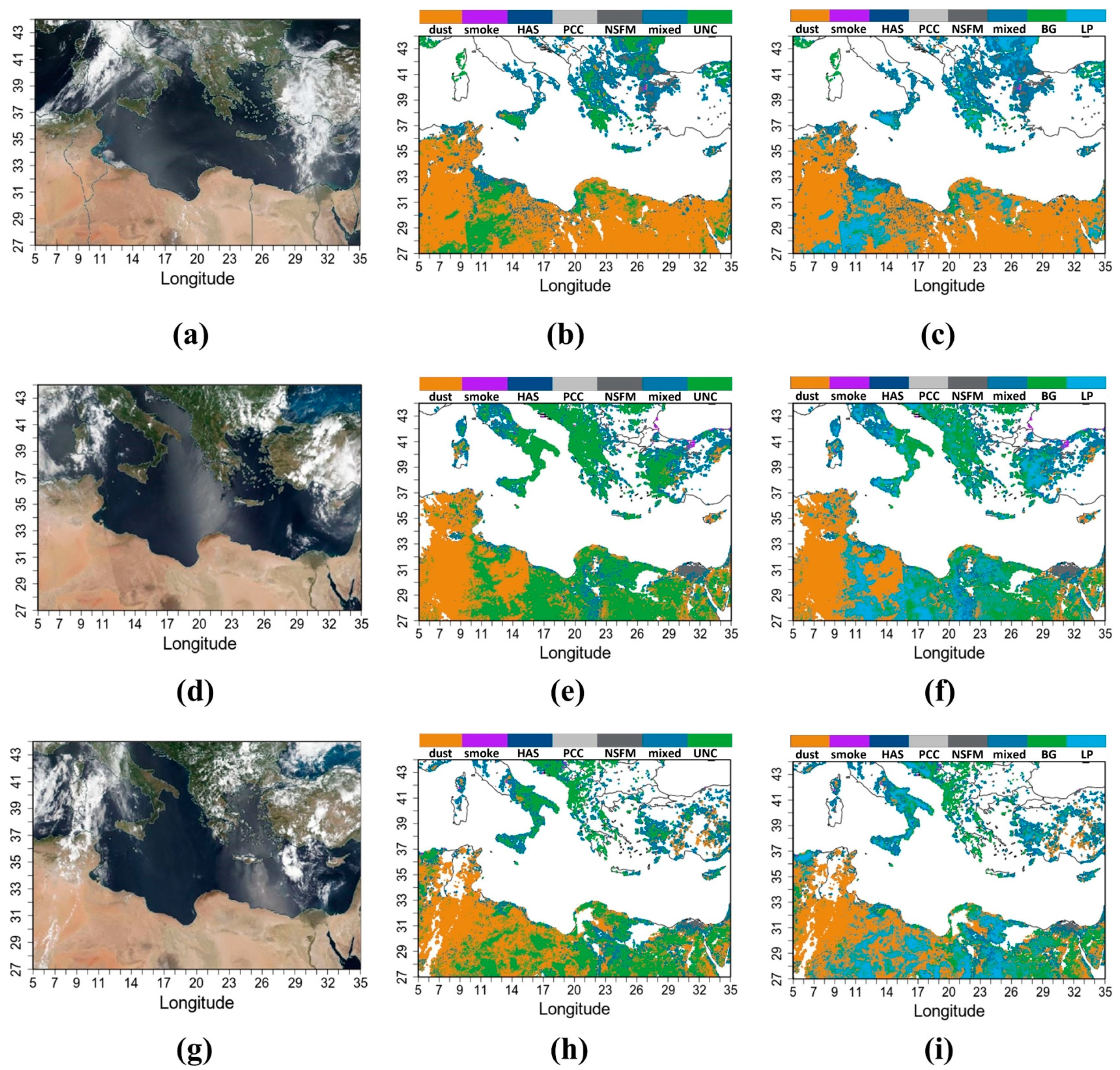
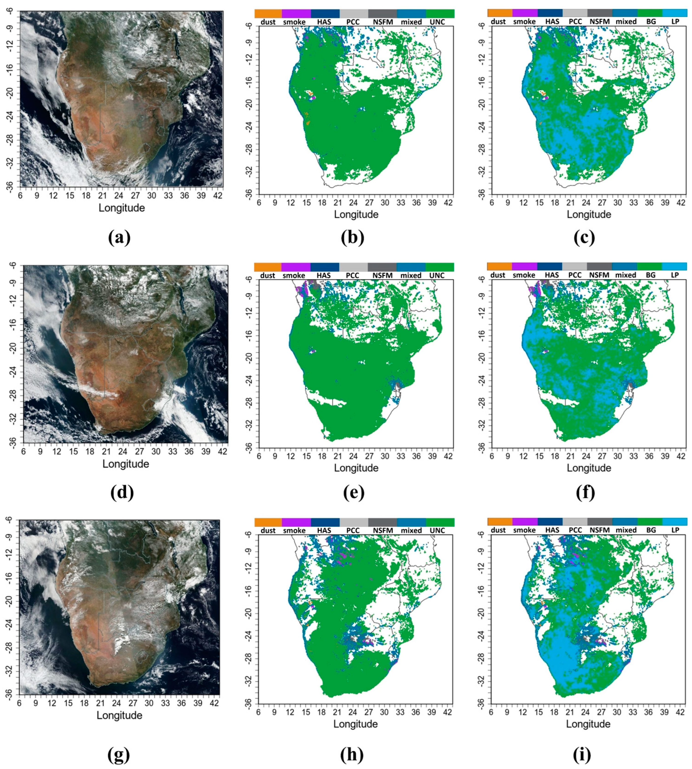
4.3. Case Studies of BAOD Applying on Satellite Aerosol Type Discrimination

For passive observations, particle radius is a key parameter in aerosol type classification, and Angstrom Exponent (AE) is a widely used parameter that describes the bulk aerosol particle size. Previous studies have proposed many well-established aerosol-type classification methods via ground-based datasets [39,40,41], but they are not applicable in low aerosol loading conditions because the key parameter, SSA, can only be accurately measured or retrieved when AOD is high (e.g., AOD > 0.4 for AERONET inversion product) [28]. Alternatively, the AOD-AE scheme is often used to achieve a rough classification in low aerosol loading conditions [42]. For ground observations, both AOD and AE can be accurately obtained, and aerosol types can be identified as background (continental clean), urban industry/biomass burning, dust, and mixed over land. However, the situation gets worse for satellite observations because AE can not be accurately retrieved in low aerosol loading conditions. Also, due to a lack of proper background AOD threshold value for a different region, a concession is made to simply tag the aerosol as a ‘background’ type when AOD is less than 0.3 in the current VIIRS dataset, and in fact, the aerosol type is not actually identified.

To illustrate the usefulness of BAOD in aerosol type classification, we update the VIIRS DB aerosol type classification scheme by replacing the original ‘background’ threshold of 0.3 with BAOD, and two case studies are introduced to compare their classifying results. Figure 9 shows the original and updated VIIRS aerosol-type classification schemes. In the updated scheme, the background AOD threshold value is determined dynamically with consideration of both the reference BAOD and the sensor limitation (AOD < 0.3), choosing the smaller one of BAOD and 0.3. A new aerosol type LP (Low Polluted) is introduced when AOD falls between the reference BAOD (if less than 0.3) and 0.3. This LP type represents a situation when aerosol loading is higher than the background condition with potential influence by weak aerosol sources, such as thin dust layers with AOD less than 0.3. To highlight the differences, we changed the VIIRS background aerosol type to an unknown type since VIIRS does not perform the type identification when AOD < 0.3.

The first case is a comparison of detecting thin dust layers over the Mediterranean (Figure 10). A thin dust layer can be observed above the Mediterranean region on 10 April, 26 April, and 9 June 2019 from the MODIS true color images (1st column of Figure 10). The thin yellow layer over the blue Mediterranean region is composed of suspended dust particles blown from the southwest to the northeast, and the white pixels are clouds. AODs over the north part of this region are generally below 0.3. Thus, the original VIIRS typing scheme reports a UNK (VIIRS background) aerosol type over these areas and loses sight of the thin dust layers (2nd column of Figure 10). However, the thin dust layers can generally be detected via the updated typing scheme as LP type, which uses BAOD as the background threshold value (3rd column of Figure 10).

The second case is a comparison of detecting thin smoke layers over South Africa (Figure 11). The thin smoke layer (gray) can be easily distinguished from the cloud (white) on 3 days in May 2019 (1st column of Figure 11). AODs over most of South Africa in the selected days are generally below 0.3. Thus, the original VIIRS typing scheme reports a ‘background’ aerosol type over this region and fails to identify the thin smoke layers (2nd column of Figure 11). However, using the updated typing scheme developed in this study, the smoke layers can be well detected as LP type (3rd column of Figure 11). From these two dust and smoke case studies, it is clear that the BAOD determined in this study is useful in detecting aerosol-type variations when AOD is lower than 0.3, which cannot be achieved using a unified background threshold of 0.3.

4.4. Definitions and Identification of Background Aerosols

The definitions of background aerosol in the previous AOD-AE scheme, the current VIIRS DB algorithm, and our study are different. Specifically, the background aerosol used in many previous AOD-AE schemes usually refers to a remote clean continental aerosol type away from anthropogenic influence (hereafter BG-RM), while the background aerosol in the VIIRS DB algorithm is more like an unknown aerosol type. The background aerosol in this study represents a local common aerosol condition without impact from transported aerosols or occasional emission events like wildfires, and it changes with locations. For example, in remote locations, the background aerosol has the same definition as BG-RM; in urban regions, it represents the daily urban/industrial aerosols without influence from dust or wildfire events or pollution episodes; and in the desert region, it refers to the natural dust aerosol.

Many previous studies used a threshold value for background type classification at a single site, and the background aerosol in these studies is similar to BG-RM. However, when classifying aerosol type at a large domain, a unified threshold value may not be proper because background aerosol types for different locations may be different, leading to different background aerosol loadings. For example, Yu, et al. [43] used 0.2 as a background threshold value to classify aerosol types in the urban Beijing area. For a clean region like the Tibetan Plateau, however, a unified threshold of 0.2 will lead to a severe loss of aerosol-type information. Thus, Pokharel, Guang, Liu, Kang, Ma, Holben, Xia, Xin, Ram, Rupakheti, Wan, Wu, Bhattarai, Zhao and Cong [42] chose a much smaller value of 0.05 as a background threshold value to catch the aerosol-type variations. This indicates that background aerosol type and its corresponding aerosol loading should vary with locations. Thus, a location-specified threshold value may be more reasonable to represent local ‘clean’ conditions (background aerosol). On a global scale, Zhang, Kondragunta, Laszlo, Liu, Remer, Huang, Superczynski and Ciren [6] used the lowest 5th percentile AOD as a background threshold value and Xia [44] used the lowest 25 percentile as a background threshold value, but their selections tend to be personal experience or preference. Based on a statistical basis in this study, we recommend the lowest 30th percentile AOD as the best background threshold value.

Although changing the background threshold value from unified 0.3 to 30th percentiles does not introduce further information regarding the aerosol type (available information for typing aerosol is still AOD and AE, and AE is unreliable when AOD is less than 0.3), it does help to identify possible aerosol type changes in a location with low AOD. The reason is that the BAOD value obtained from the statistical process can be regarded as a priori knowledge of local common aerosol loading. When AOD is lower than BAOD, the aerosol generally represents the local background type. When AOD at a certain location is higher than BAOD, it means that the particular region is influenced by biomass burning, pollution, or dust episodes. Consequently, the local aerosol type may change from background to some other types, e.g., smoke or dust. In other words, the 30th percentile itself contains local background aerosol loading information. Thus, background aerosol can be identified by comparing AOD and BAOD without the use of AE, which becomes unreliable under low AOD conditions.

The multiple models in the AOD histogram can be a representation of aerosol species. A relatively large increase or decrease in AOD is mostly related to the change in local aerosol type. For a specific location, for example, Los Angeles, the background aerosol type should be urban/industrial type without transported aerosols (e.g., smoke or dust), and its AOD histogram tends to be a mono-normal distribution. When wildfire happens, however, AOD increases sharply, and a peak appears toward a larger AOD end. If dust aerosols or pollutants are transported into the area, aerosol loading will also increase, and another peak may appear. Therefore, the first peak could be representative of local background aerosol, but the later peaks are influenced by the transported pollutants or unusual local emissions like wildfires. However, what these later peaks represent or which kind of aerosol they are (e.g., dust, smoke, or some kind of mixture) needs further in-depth analysis because it may vary substantially from location to location.

5. Conclusions

This study develops a statistical method to determine global background AOD threshold values using the VIIRS AOD product. The 30th percentile of the lowest AOD is found to be the best estimation of BAOD for multiple datasets and different seasons. According to the multiple lognormal fitting, quadruple and triple lognormal modes are found to occur most frequently around the world, indicating a distinct aerosol-type variation on a global scale. A high BAOD value of over 0.4 appears in North and Mid Africa, the Arabian Peninsula, North and Mid Africa, and the northern part of South America, while other regions generally have a BAOD value of less than 0.1. The original VIIRS dataset left 80% of observations (AOD < 0.3) unclassified in low aerosol loading regions like America, Europe, and Australia and tagged them as a ‘background’ type; thus, the aerosol type information for low AOD remains unknown in the original VIIRS aerosol type classification scheme.

Chemical component information from MERRA-2 is involved in examining the selection of the 30th percentile of the lowest AOD as the BAOD threshold value. On a global scale, aerosol chemical components vary slightly when AOD is lower than BAOD, while the degree and rate of change of aerosol chemical components gradually become strong and significant when AOD is greater than BAOD. And the breaking point of the changing trend coincides with our statistical results properly.

Based on the reference BAOD threshold value, we update the AOD-AE aerosol type classification scheme. We redefine the background type and introduce a new aerosol-type cluster, low polluted (LP), into the classification scheme. Through two dust and smoke case studies, it is clear that our updated AOD-AE scheme is able to achieve a pretty good detection of aerosol type changes in low aerosol loading conditions, and it can give us a better view of aerosol type variation for VIIRS-like passive sensors over low aerosol loadings regions like America, Europe, and Australia.

There are also some limitations that should be concluded. VIIRS AOD performs relatively worse over low AOD areas, such as the highly elevated Tibetan Plateau in western China. This can lead to biased BAOD threshold value estimation. Although BAOD provides more details about the variation of aerosol types under low aerosol loading conditions from satellite observation, it is still insufficient to quantitatively identify the specific aerosol particles that cause an increase in aerosol loading above the BAOD threshold when the overall AOD is lower than 0.3. Future efforts will focus on improving the performance of satellite inversion algorithms over rugged mountain regions. Additionally, detailed identification of aerosol types under low aerosol loading conditions may be achieved by including polarized observations or chemical information from real-time model simulations, with possible assistance from machine learning.

References

1. Cai, H.; Yang, Y.; Luo, W.; Chen, Q. City-level variations in aerosol optical properties and aerosol type identification derived from long-term MODIS/Aqua observations in the Sichuan Basin, China. Urban Clim. 2021, 38, 100886. [Google Scholar] [CrossRef]
2. Zhao, B.; Wang, Y.; Gu, Y.; Liou, K.-N.; Jiang, J.H.; Fan, J.; Liu, X.; Huang, L.; Yung, Y.L. Ice nucleation by aerosols from anthropogenic pollution. Nat. Geosci. 2019, 12, 602–607. [Google Scholar] [CrossRef] [PubMed]
3. Hsu, N.C.; Lee, J.; Sayer, A.M.; Kim, W.; Bettenhausen, C.; Tsay, S.C. VIIRS Deep Blue Aerosol Products Over Land: Extending the EOS Long-Term Aerosol Data Records. J. Geophys. Res. Atmos. 2019, 124, 4026–4053. [Google Scholar] [CrossRef]
4. Crippa, P.; Sullivan, R.C.; Thota, A.; Pryor, S.C. Sensitivity of Simulated Aerosol Properties Over Eastern North America to WRF-Chem Parameterizations. J. Geophys. Res. Atmos. 2019, 124, 3365–3383. [Google Scholar] [CrossRef]
5. Gao, J.; Li, Y.; Xie, Z.; Wang, L.; Hu, B.; Bao, F. Which aerosol type dominate the impact of aerosols on ozone via changing photolysis rates? Sci. Total Environ. 2023, 854, 158580. [Google Scholar] [CrossRef] [PubMed]
6. Zhang, H.; Kondragunta, S.; Laszlo, I.; Liu, H.; Remer, L.A.; Huang, J.; Superczynski, S.; Ciren, P. An enhanced VIIRS aerosol optical thickness (AOT) retrieval algorithm over land using a global surface reflectance ratio database. J. Geophys. Res. Atmos. 2016, 121, 10717–10738. [Google Scholar] [CrossRef]
7. Bao, F.; Li, Y.; Gao, J. Carbonaceous aerosols remote sensing from geostationary satellite observation, Part I: Algorithm development using critical reflectance. Remote Sens. Environ. 2023, 287, 113459. [Google Scholar] [CrossRef]
8. Dubovik, O.; Holben, B.; Eck, T.F.; Smirnov, A.; Kaufman, Y.J.; King, M.D.; Tanré, D.; Slutsker, I. Variability of absorption and optical properties of key aerosol types observed in worldwide locations. J. Atmos. Sci. 2002, 59, 590–608. [Google Scholar] [CrossRef]
9. Chen, A.; Zhao, C.; Shen, L.; Fan, T. Influence of aerosol properties and surface albedo on radiative forcing efficiency of key aerosol types using global AERONET data. Atmos. Res. 2023, 282, 106519. [Google Scholar] [CrossRef]
10. Eom, S.; Kim, J.; Lee, S.; Holben, B.N.; Eck, T.F.; Park, S.-B.; Park, S.S. Long-term variation of aerosol optical properties associated with aerosol types over East Asia using AERONET and satellite (VIIRS, OMI) data (2012–2019). Atmos. Res. 2022, 280, 106457. [Google Scholar] [CrossRef]
11. Xia, X.; Che, H.; Zhu, J.; Chen, H.; Cong, Z.; Deng, X.; Fan, X.; Fu, Y.; Goloub, P.; Jiang, H.; et al. Ground-based remote sensing of aerosol climatology in China: Aerosol optical properties, direct radiative effect and its parameterization. Atmos. Environ. 2016, 124, 243–251. [Google Scholar] [CrossRef]
12. Petrenko, M.; Kahn, R.; Chin, M.; Limbacher, J. Refined Use of Satellite Aerosol Optical Depth Snapshots to Constrain Biomass Burning Emissions in the GOCART Model. J. Geophys. Res. Atmos. 2017, 122, 10983–11004. [Google Scholar] [CrossRef]
13. Chen, Q.-X.; Shen, W.-X.; Yuan, Y.; Tan, H.-P. Verification of aerosol classification methods through satellite and ground-based measurements over Harbin, Northeast China. Atmos. Res. 2019, 216, 167–175. [Google Scholar] [CrossRef]
14. Zhang, L.; Li, J. Variability of Major Aerosol Types in China Classified Using AERONET Measurements. Remote Sens. 2019, 11, 2334. [Google Scholar] [CrossRef]
15. Zheng, Y.; Che, H.; Xia, X.; Wang, Y.; Yang, L.; Chen, J.; Wang, H.; Zhao, H.; Li, L.; Zhang, L.; et al. Aerosol optical properties and its type classification based on multiyear joint observation campaign in north China plain megalopolis. Chemosphere 2021, 273, 128560. [Google Scholar] [CrossRef] [PubMed]
16. Kalapureddy, M.C.R.; Kaskaoutis, D.G.; Ernest Raj, P.; Devara, P.C.S.; Kambezidis, H.D.; Kosmopoulos, P.G.; Nastos, P.T. Identification of aerosol type over the Arabian Sea in the premonsoon season during the Integrated Campaign for Aerosols, Gases and Radiation Budget (ICARB). J. Geophys. Res. Atmos. 2009, 114, D17203. [Google Scholar] [CrossRef]
17. Lee, J.; Kim, J.; Song, C.H.; Kim, S.B.; Chun, Y.; Sohn, B.J.; Holben, B.N. Characteristics of aerosol types from AERONET sunphotometer measurements. Atmos. Environ. 2010, 44, 3110–3117. [Google Scholar] [CrossRef]
18. Cappa, C.D.; Kolesar, K.R.; Zhang, X.; Atkinson, D.B.; Pekour, M.S.; Zaveri, R.A.; Zelenyuk, A.; Zhang, Q. Understanding the optical properties of ambient sub- and supermicron particulate matter: Results from the CARES 2010 field study in northern California. Atmos. Chem. Phys. 2016, 16, 6511–6535. [Google Scholar] [CrossRef]
19. Cao, C.; Xiong, J.; Blonski, S.; Liu, Q.; Uprety, S.; Shao, X.; Bai, Y.; Weng, F. Suomi NPP VIIRS sensor data record verification, validation, and long-term performance monitoring. J. Geophys. Res. Atmos. 2013, 118, 11664–11678. [Google Scholar] [CrossRef]
20. Sayer, A.; Hsu, N.; Bettenhausen, C.; Jeong, M.-J. Validation and uncertainty estimates for MODIS Collection 6 “Deep Blue” aerosol data. J. Geophys. Res. Atmos. 2013, 118, 7864–7872. [Google Scholar] [CrossRef]
21. Chen, X.; Ding, H.; Li, J.; Wang, L.; Li, L.; Xi, M.; Zhao, L.; Shi, Z.; Liu, Z. Remote sensing retrieval of aerosol types in China using geostationary satellite. Atmos. Res. 2024, 299, 107150. [Google Scholar] [CrossRef]
22. Vadde, S.; Kalluri, R.O.R.; Gugamsetty, B.; Kotalo, R.G.; Kajjer Virupakshappa, U.; Akkiraju, B.; Thotli, L.R.; Lingala, S.S.R.; Rapole, J.K. Classifying aerosol type using in situ and satellite observations over a semi-arid station, Anantapur, from southern peninsular India. Adv. Space Res. 2023, 72, 1109–1122. [Google Scholar] [CrossRef]
23. Khademi, F.; Bayat, A. Classification of aerosol types using AERONET version 3 data over Kuwait City. Atmos. Environ. 2021, 265, 118716. [Google Scholar] [CrossRef]
24. Zhao, H.; Gui, K.; Ma, Y.; Wang, Y.; Wang, Y.; Wang, H.; Zheng, Y.; Li, L.; Zhang, L.; Che, H.; et al. Climatological variations in aerosol optical depth and aerosol type identification in Liaoning of Northeast China based on MODIS data from 2002 to 2019. Sci. Total Environ. 2021, 781, 146810. [Google Scholar] [CrossRef]
25. Zhou, P.; Wang, Y.; Liu, J.; Xu, L.; Chen, X.; Zhang, L. Difference between global and regional aerosol model classifications and associated implications for spaceborne aerosol optical depth retrieval. Atmos. Environ. 2023, 300, 119674. [Google Scholar] [CrossRef]
26. Cao, C.; Luccia, F.J.D.; Xiong, X.; Wolfe, R.; Weng, F. Early On-Orbit Performance of the Visible Infrared Imaging Radiometer Suite Onboard the Suomi National Polar-Orbiting Partnership (S-NPP) Satellite. IEEE Trans. Geosci. Remote Sens. 2014, 52, 1142–1156. [Google Scholar] [CrossRef]
27. Eck, T.F.; Holben, B.N.; Giles, D.M.; Slutsker, I.; Sinyuk, A.; Schafer, J.S.; Smirnov, A.; Sorokin, M.; Reid, J.S.; Sayer, A.M.; et al. AERONET Remotely Sensed Measurements and Retrievals of Biomass Burning Aerosol Optical Properties During the 2015 Indonesian Burning Season. J. Geophys. Res. Atmos. 2019, 124, 4722–4740. [Google Scholar] [CrossRef]
28. Giles, D.M.; Sinyuk, A.; Sorokin, M.G.; Schafer, J.S.; Smirnov, A.; Slutsker, I.; Eck, T.F.; Holben, B.N.; Lewis, J.R.; Campbell, J.R.; et al. Advancements in the Aerosol Robotic Network (AERONET) Version 3 database—Automated near-real-time quality control algorithm with improved cloud screening for Sun photometer aerosol optical depth (AOD) measurements. Atmos. Meas. Tech. 2019, 12, 169–209. [Google Scholar] [CrossRef]
29. Qiao, Y.; Ji, D.; Shang, H.; Xu, J.; Xu, R.; Shi, C. The Fusion of ERA5 and MERRA-2 Atmospheric Temperature Profiles with Enhanced Spatial Resolution and Accuracy. Remote Sens. 2023, 15, 3592. [Google Scholar] [CrossRef]
30. Liu, C.; Yin, Z.; He, Y.; Wang, L. Climatology of Dust Aerosols over the Jianghan Plain Revealed with Space-Borne Instruments and MERRA-2 Reanalysis Data during 2006–2021. Remote Sens. 2022, 14, 4414. [Google Scholar] [CrossRef]
31. Ignatov, A.; Holben, B.; Eck, T. The lognormal distribution as a reference for reporting aerosol optical depth statistics; Empirical tests using multi-year, multi-site AERONET Sunphotometer data. Geophys. Res. Lett. 2000, 27, 3333–3336. [Google Scholar] [CrossRef]
32. Povey, A.; Grainger, R. Towards more representative gridded satellite products. IEEE Geosci. Remote Sens. Lett. 2018, 16, 672–676. [Google Scholar] [CrossRef]
33. Łukaszyk, S. A new concept of probability metric and its applications in approximation of scattered data sets. Comput. Mech. 2004, 33, 299–304. [Google Scholar] [CrossRef]
34. Wylie, D.; Jackson, D.L.; Menzel, W.P.; Bates, J.J. Trends in Global Cloud Cover in Two Decades of HIRS Observations. J. Clim. 2005, 18, 3021–3031. [Google Scholar] [CrossRef]
35. Sayer, A.M.; Hsu, N.C.; Lee, J.; Kim, W.V.; Dutcher, S.T. Validation, stability, and consistency of MODIS collection 6.1 and VIIRS version 1 Deep Blue aerosol data over land. J. Geophys. Res. Atmos. 2019, 124, 4658–4688. [Google Scholar] [CrossRef]
36. Reid, J.S.; Hyer, E.J.; Johnson, R.S.; Holben, B.N.; Yokelson, R.J.; Zhang, J.; Campbell, J.R.; Christopher, S.A.; Di Girolamo, L.; Giglio, L.; et al. Observing and understanding the Southeast Asian aerosol system by remote sensing: An initial review and analysis for the Seven Southeast Asian Studies (7SEAS) program. Atmos. Res. 2013, 122, 403–468. [Google Scholar] [CrossRef]
37. Zhao, B.; Jiang, J.H.; Diner, D.J.; Su, H.; Gu, Y.; Liou, K.-N.; Jiang, Z.; Huang, L.; Takano, Y.; Fan, X.; et al. Intra-annual variations of regional aerosol optical depth, vertical distribution, and particle types from multiple satellite and ground-based observational datasets. Atmos. Chem. Phys. 2018, 18, 11247–11260. [Google Scholar] [CrossRef] [PubMed]
38. Gao, M.; Han, Z.; Tao, Z.; Li, J.; Kang, J.E.; Huang, K.; Dong, X.; Zhuang, B.; Li, S.; Ge, B.; et al. Air quality and climate change, Topic 3 of the Model Inter-Comparison Study for Asia Phase III (MICS-Asia III)—Part 2: Aerosol radiative effects and aerosol feedbacks. Atmos. Chem. Phys. 2020, 20, 1147–1161. [Google Scholar] [CrossRef]
39. Bibi, H.; Alam, K.; Bibi, S. In-depth discrimination of aerosol types using multiple clustering techniques over four locations in Indo-Gangetic plains. Atmos. Res. 2016, 181, 106–114. [Google Scholar] [CrossRef]
40. Schmeisser, L.; Andrews, E.; Ogren, J.A.; Sheridan, P.; Jefferson, A.; Sharma, S.; Kim, J.E.; Sherman, J.P.; Sorribas, M.; Kalapov, I.; et al. Classifying aerosol type using in situ surface spectral aerosol optical properties. Atmos. Chem. Phys. 2017, 17, 12097–12120. [Google Scholar] [CrossRef]
41. Shin, S.K.; Tesche, M.; Noh, Y.; Müller, D. Aerosol-type classification based on AERONET version 3 inversion products. Atmos. Meas. Tech. 2019, 12, 3789–3803. [Google Scholar] [CrossRef]
42. Pokharel, M.; Guang, J.; Liu, B.; Kang, S.; Ma, Y.; Holben, B.N.; Xia, X.A.; Xin, J.; Ram, K.; Rupakheti, D.; et al. Aerosol Properties Over Tibetan Plateau from a Decade of AERONET Measurements: Baseline, Types, and Influencing Factors. J. Geophys. Res. Atmos. 2019, 124, 13357–13374. [Google Scholar] [CrossRef]
43. Yu, X.; Kumar, K.R.; Lü, R.; Ma, J. Changes in column aerosol optical properties during extreme haze-fog episodes in January 2013 over urban Beijing. Environ. Pollut. 2016, 210, 217–226. [Google Scholar] [CrossRef] [PubMed]
44. Xia, X. Variability of aerosol optical depth and Angstrom wavelength exponent derived from AERONET observations in recent decades. Environ. Res. Lett. 2011, 6, 044011. [Google Scholar] [CrossRef]
Figure 1. Determination of background AOD threshold value for different AOD histogram situations. (a) fitted mono mode, and (b) fitted multiple modes. Here, two AERONET AOD histograms from Karlsruhe and Georgia Tech are used as an example to illustrate the determination of BAOD threshold value for the mono- and multi-lognormal distributions.
Remotesensing 16 01210 g001
Figure 2. (a) Map of the available VIIRS DB AOD observations from March 2012 to December 2019 and the correlations with AERONET measurements, circles denote the involved AERONET sites, the vertical color bar denotes the magnitude of the correlation, and the horizontal color bar denotes the VIIRS DB AOD observation number during the study period; (b) the overall correlation between VIIRS DB and AERONET AOD. EE represents estimated error; the 1:1 line is shown in black dotted line; the gray dotted lines indicate ±(0.05 + 15%) of the AERONET AOD; and (c) Annual mean DB AOD map at 550 nm from VIIRS measurements during March 2012 to February 2019. (d) performance of VIIRS DB for different AOD bins.
Remotesensing 16 01210 g002
Figure 3. VIIRS DB AOD map at different lowest percentile, from (ag) 3rd, 16th, 25th, 50th, 75th, 83rd, and 97th percentile.
Remotesensing 16 01210 g003aRemotesensing 16 01210 g003b
Figure 4. (a) Multiple lognormal fitting correlation map and fitted ratios for different lognormal modes, and (b) preliminary BAOD map at 550 nm.
Remotesensing 16 01210 g004
Figure 5. (a) Variation of the BAOD bias with lowest AOD percentiles at 550 nm from VIIRS, (b) global map of the 30th percentile of the lowest AOD at 550 nm as the background threshold value, (c) The AERONET interpolated BAOD from inverse distance weight interpolation.
Remotesensing 16 01210 g005
Figure 6. Variation of the BAOD bias with lowest AOD percentiles at 550 nm from (a) Terra-MODIS DT, (b) Terra-MODIS DB, (c) Terra-MODIS DTB, (d) Aqua-MODIS DT, (e) Aqua-MODIS DB, (f) Aqua-MODIS DTB, (g) MISR and (h) Terra-MODIS DB in June during 2012–2019.
Remotesensing 16 01210 g006
Figure 7. Variations of the normalized standard deviation of column aerosol mass density, blue and red refer to low and high value of normalized standard deviation, respectively.
Remotesensing 16 01210 g007
Figure 8. Slope of the normalized standard deviations of the column mass densities. Note the y-coordinate ranges are different, and white and red refer to low and high value of slope of the normalized standard deviation, respectively.
Remotesensing 16 01210 g008aRemotesensing 16 01210 g008b
Figure 9. Flowchart illustrating the aerosol type classification scheme over land in the VIIRS DB algorithm. The yellow boxes represent the original scheme, and the blue boxes represent the updated scheme of this study.
Remotesensing 16 01210 g009
Figure 10. VIIRS RGB images of three dust events over the Mediterranean in (a) April 26th, (d) 9th June, and (g) 10th April 2019. Corresponding aerosol type classification results from VIIRS original AOD-AE scheme are shown in (b,e,h), and the results from the updated scheme are shown in (c,f,i). HAS, NSFM, UNK, BG, and LP represent the high altitude smoke, non-smoke fine mode, unknown, background, and low pollution in low aerosol loading, respectively.
Remotesensing 16 01210 g010
Figure 11. Similar to Figure 10, but for three biomass-burning events over South Africa on 19th May (ac), 21st (df), and 24th (gi), 2019. HAS, NSFM, UNK, BG, and LP represent the high altitude smoke, non-smoke fine mode, unknown, background, and low pollution in low aerosol loading, respectively.
Remotesensing 16 01210 g011