Abstract
Road extraction is a crucial aspect of remote sensing imagery processing that plays a significant role in various remote sensing applications, including automatic driving, urban planning, and path navigation. However, accurate road extraction is a challenging task due to factors such as high road density, building occlusion, and complex traffic environments. In this study, a Spatial Attention Swin Transformer (SASwin Transformer) architecture is proposed to create a robust encoder capable of extracting roads from remote sensing imagery. In this architecture, we have developed a spatial self-attention (SSA) module that captures efficient and rich spatial information through spatial self-attention to reconstruct the feature map. Following this, the module performs residual connections with the input, which helps reduce interference from unrelated regions. Additionally, we designed a Spatial MLP (SMLP) module to aggregate spatial feature information from multiple branches while simultaneously reducing computational complexity. Two public road datasets, the Massachusetts dataset and the DeepGlobe dataset, were used for extensive experiments. The results show that our proposed model has an improved overall performance compared to several state-of-the-art algorithms. In particular, on the two datasets, our model outperforms D-LinkNet with an increase in Intersection over Union (IoU) metrics of 1.88% and 1.84%, respectively.
1. Introduction
Road extraction from remote sensing imagery is one of the important research topics in remote sensing applications. It provides significant convenience for areas such as autonomous driving, vehicle navigation [1], and urban planning [2]. With the rapid development of urban and rural areas, detecting the latest road surface becomes an important and challenging task. The manual labeling of roads is a time-consuming and labor-intensive task, especially when dealing with large areas of road network coverage. Therefore, how to use efficient algorithms to inversion road networks from remote sensing imagery is a problem of great interest in the academic community.
The existing methods can be summarized into four categories: traditional methods, convolutional neural network (CNN)-based methods, Transformer-based methods, and graph-based methods. (1) Traditional research in this field has mainly focused on analyzing low-resolution remote sensing images and Global Positioning System (GPS) data using manually designed features and defining specific criteria to extract roads [3,4,5]. However, these methods often perform inefficiently and may not achieve satisfactory results when dealing with large-area, high-resolution satellite images. (2) Convolutional neural networks (CNNs), especially networks with fully convolutional network [6] architectures, have been proposed and proven effective in image semantic segmentation [7,8,9,10,11,12]. Neural networks based on encoder–decoder architectures [13,14,15,16,17] have achieved satisfactory results in image segmentation. However, these CNN-based methods only focus on local feature information, which can lead to difficulties in detecting roads that are obstructed by buildings and vehicles, resulting in fragmented road segmentation. (3) In recent years, Transformer-based methods [18,19,20,21,22] have made significant progress in image classification and segmentation. Unlike previous CNN-based methods, Transformers are powerful in establishing long-range dependencies and demonstrate excellent transferability in downstream tasks under large-scale pre-training. However, roads have the characteristics of long spans, narrow widths, and continuous distributions, and the number of pixels belonging to roads relative to non-road pixels in a satellite image is relatively small. Therefore, Transformers may lead to unnecessary computations and reduce segmentation accuracy when modeling in a global context. (4) Graph-based methods [23,24,25,26,27] are capable of effectively capturing the spatial relationships and topological structures among pixels in road images. However, they may require a longer computation time and larger computing resources when dealing with large-scale image data, particularly in complex scenarios such as high-resolution images or images with a significant number of traffic objects.
In this paper, we propose a SASwin Transformer for extracting road information from remote sensing imagery. We introduce an encoder architecture based on the joint learning of Swin Transformer [28] and ResNet [29] to learn road features. To reduce unnecessary computations that may result from modeling a global context with Swin Transformer and considering the characteristics of roads with large spans, narrow widths, and continuous distributions, we improve the multi-head self-attention (MSA) in the Swin Transformer and design an SSA module to capture more efficient spatial information. We also enhance the MLP in the Swin Transformer and develop an SMLP module to aggregate spatial feature information from multiple branches while reducing computational complexity. The contributions of this work can be summarized as follows:
- We propose a SASwin Transformer network that jointly learns global and local feature information from satellite images to enhance road segmentation.
- We have developed an SMLP module that aggregates rich spatial context information by performing linear transformations in three dimensions of the image. Compared to the original MLP module, this SMLP module reduces computational complexity.
- We have designed an SSA module to extract effective spatial context information. Compared to the original MSA module, it reduces unnecessary computations and avoids interference from irrelevant regions.
- Compared to other advanced methods, our approach achieves significant improvements in segmentation accuracy. On two publicly available datasets, our method outperforms D-LinkNet by 1.88% and 1.84% in terms of the IoU metric.
The rest of this paper is organized as follows. Section 2 summarizes related work on road extraction. In Section 3, we describe the details of our proposed SASWin Transformer. Section 4 provides the dataset, evaluation metrics, and implementation details and conducts extensive experiments to evaluate the performance of our proposed method. The conclusion and discussion are presented in Section 5.
2. Related Work
2.1. Conventional Methods
Many studies have attempted to extract road information from remote sensing imagery. Ref. [30] designed a road extraction algorithm based on a color model by combining boundary information on grayscale images and road region extraction results on color images. Ref. [31] extracted road regions by analyzing the texture features of the road and extracting them based on different texture characteristics. Ref. [32] used a higher-order conditional random field (CRF) model for road extraction. Ref. [33] also proposed a two-stage model. First, the pixels are divided into road and non-road groups using a support vector machine (SVM) algorithm based on road features. Second, the road group is refined using segmentation algorithms to generate the final road regions. The advantages of these traditional methods are their simplicity and ease of implementation. However, these methods often have low efficiency and may not perform well in complex road scenarios, especially in situations where road extraction is difficult in complex scenes.
2.2. CNN-Based Methods
Since their remarkable success in the ImageNet Large Scale Visual Recognition Challenge [34] in 2012, CNNs have opened up a new era for deep learning-based image recognition. With the development of deep learning, CNNs have also been widely applied in the field of image segmentation. For example, Ref. [6] proposed the fully convolutional network (FCN), which greatly improves segmentation performance compared to some of the traditional methods that have been used in the past. Ref. [7] proposed a UNet based on an encoder–decoder architecture, where the encoder part performs feature extraction and downsampling via convolution layers and the decoder part performs upsampling via transposed convolution layers, combined with skip connections for feature fusion. This allows the high-resolution feature maps to be restored to the original image resolution and perform pixel-level predictions. Ref. [35] proposed a SegNet model. Ref. [36] proposed ResUnet, which combines residual learning with UNet for road extraction.
In the IEEE Conference on Computer Vision and Pattern Recognition (CVPR) DeepGlobe 2018 Road Extraction Challenge [37], Ref. [9] proposed a D-LinkNet model. D-LinkNet mainly addresses the limitations of traditional semantic segmentation models in handling details and edge information. It employs a deep supervision mechanism to address the feature fusion problem, thereby improving model performance. Additionally, D-LinkNet utilizes a strategy of multi-scale feature fusion to capture semantic information from multiple scales. Inspired by the shape and connectivity of roads in grid networks, Ref. [38] introduced a boosting strategy by applying multiple segmentation networks to enhance the road segmentation results. The network learns progressively from previous segmentation failure cases to connect disconnected road sections in the initial mask. To effectively combine multi-scale information and extract global feature information, Ref. [39] proposed a cross-scale, axial attention-based approach. However, these methods only focus on local information. Due to the lack of establishment of long-range dependencies, this is likely to lead to the neglect of some crucial information.
2.3. Transformer-Based Methods
Transformer was first proposed by [40] in 2017. It was initially used in natural language processing tasks and achieved state-of-the-art performance in various benchmarks. Unlike CNNs, Transformer relies entirely on self-attention mechanisms to process input sequences, enabling the parallel processing of input tokens and the capture of long-range relationships. Subsequently, many researchers have attempted to apply Transformer in the field of computer vision but did not achieve satisfactory results compared to CNNs until Ref. [41] introduced Vision Transformer (ViT) in 2020. ViT processes image data as sequence data and utilizes self-attention mechanisms to capture contextual information within the sequence. This sequential approach to image processing is different from CNNs, which heavily rely on convolutional and pooling layers to capture image features. Swin Transformer [28] is an architecture designed for processing image data. By processing image data in blocks, Swin Transformer effectively solves the computational and memory complexity problems of conventional Vision Transformers. The shifted window mechanism is introduced in each block to increase the local receptive field. Swin Transformer has been greatly improved in performance and efficiency compared to previous Vision Transformers. Ref. [42] proposed a SwinUnet model, which is the first pure Transformer-based encoder–decoder architecture without any convolution operation. In the encoder, local-to-global self-attention is implemented to capture features. In the decoder, global features are extracted and progressively upsampled, and then the corresponding pixel-level segmentation is predicted. Ref. [43] proposed Pyramid Vision Transformer (PVT), which can more effectively extract global contextual information and significantly improve the model’s segmentation performance. Research studies [44,45] show that ViT has the ability to model global contextual interactions and the flexibility to adjust the modeling capabilities of different regions. ViT has demonstrated comparable performance to traditional CNNs in benchmark tests on the ImageNet dataset, indicating its effectiveness as a solution for computer vision tasks such as image and video processing. The first application of masked image modeling (MIM) to a remote sensing road extraction task was presented by [46]. MIM improves the region interaction by reconstructing masked regions from unmasked regions. This is comparable to the process of deducing masked road regions from remotely sensed images in a road extraction task.
2.4. Combining CNN with Transformer
Although the ability of Transformer models to capture long-range dependencies has led to improvements in segmentation performance in image segmentation tasks, convolutional neural networks still have a natural advantage in capturing local feature information. Recently, in the field of road extraction research, attempts have been made to combine Transformers and CNNs. These methods have both the ability of Transformers to capture long-range dependencies and the ability of CNNs to capture local feature information. To combine the advantages of both the CNN and Transformer architectures, Ref. [47] proposed a Conformer, which designs a dual-path structure that allows them to interactively learn features. The experiments showed that the performance of the mixed CNN–Transformer encoder is better than that of using Transformer alone as the encoder. Ref. [48] proposed a TransUNet model, which combines the characteristics of Transformer and UNet. It first uses CNNs to extract features from images to obtain feature maps, which are then transformed and input to the Transformer encoder module. Finally, it uses a decoder module similar to that of U-Net to perform layer-wise upsampling and skip connections to generate segmentation maps. This model has achieved good results on multiple image segmentation tasks. Ref. [49] extended Swin Transformer and added decoder structures to improve the road segmentation performance of the model. Ref. [50] proposed the Seg-Road model to enhance road connectivity. The model utilizes a Transformer to establish long-distance dependencies and global contextual information to enhance the fragmentation of road segmentation. Additionally, it employs a CNN structure to extract local context information to improve the segmentation of road details.
3. The Proposed SASwin Transformer Method
In this section, the Spatial Attention Swin Transformer (SASWin Transformer) network for road extraction from remote sensing imagery is detailed, as shown in Figure 1. In order to extract features more comprehensively and improve segmentation performance, we have developed an SMLP module to aggregate rich spatial contextual information and designed an SSA module to reduce unnecessary computations and avoid interference from irrelevant regions.
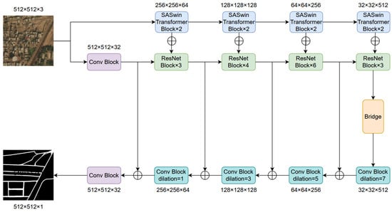
Figure 1.
The overall architecture of the proposed Spatial Attention Swin Transformer (SASwin Transformer) is as follows. The encoder module consists of five convolutional blocks. The bridge module learns multi-scale features by applying multi-scale dilated convolutions. The decoder module includes five convolutional blocks.
3.1. Overall Network Structure
The framework of SASWin includes three modules: encoder, bridge, and decoder.
3.1.1. Encoder Module
In the encoder module, we introduce a Spatial Swin Transformer and ResNet as dual encoders to extract feature information. Since ResNet mainly focuses on local information during the process of feature encoding, which can lead to the loss of a significant amount of critical information as the network depth deepens and the image resolution gradually decreases, we will incorporate the Swin Transformer into the encoder, which excels in its ability to establish long-range dependency relationships. Considering that roads have features of long spans, narrowness, and continuous distribution and that the pixels belonging to roads in a satellite image are relatively few compared to the non-road pixels, we have improved the MLP and MSA architectures in the Swin Transformer to enable more effective feature extraction.
3.1.2. Bridge Module
We introduce the bridge module to conduct multi-scale feature learning and increase the range of local feature perception. The bridge module is shown in Figure 2. Considering the long span and narrow characteristics of the road, we used , , and convolutions to more effectively extract local feature information. Then, each output feature is adjusted through convolution, and finally, the final feature map is outputted through convolution. To increase the range of local feature perception, we used dilated convolutions with dilation rates of 8, 4, and 2, respectively, to extract feature information step by step.
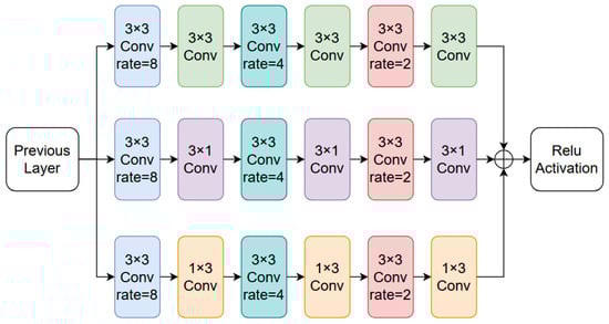
Figure 2.
Previous layer refers to the encoder network portion in Figure 1, which finally outputs a data tensor of the same dimension as the input after being activated by the Relu activation function.
3.1.3. Decoder Module
We introduce the decoder module to generate segmentation results. Due to the ability of dilated convolutions to increase the receptive field size of the convolutional kernel while maintaining the spatial dimensions of the input and output, neural networks can better capture global information and contextual relationships in the input feature maps. Therefore, we applied dilated convolutions with dilation rates of 7, 5, 3, and 1 to the four convolutional blocks in the decoder, enabling more dense feature extraction. The output of the model is a raster with a number of channels of 1 and a size of 512 × 512. These 512 × 512 pixels are classified as road pixels and non-road pixels, respectively.
3.2. SASwin Transformer Blocks
Let be the input of the network, where H, W, and C represent the height, width, and number of channels, respectively. , , , and are the outputs of every two successive SASwin Transformer blocks. As shown in Figure 3, continuous SASwin Transformer blocks are computed using the shift window partition method as follows:
where and , respectively, represent the output features of the (S)W-SSA module and SMLP module in block l. W-SSA and SW-SSA are both window-based spatial self-attention modules. W-SSA uses the window partitioning rules from Swin Transformer, while SW-SSA uses the shifting window rules from Swin Transformer.
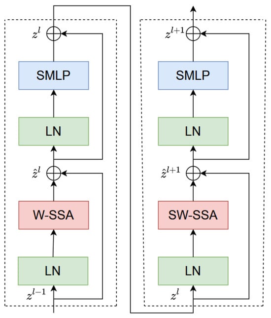
Figure 3.
Two successive SASwin Transformer blocks.
3.3. Spatial MLP Module
We have designed a Spatial MLP (SMLP) to alleviate the two main drawbacks of the original MLP. Firstly, by reducing the number of parameters, we can avoid the overfitting problem, especially when dealing with large-scale datasets. Secondly, by reducing computational complexity, particularly when dealing with a large number of tokens, we can achieve multi-stage processing in the pyramid structure.
In the SMLP module, the tokens of the SMLP only interact directly with the tokens on the same row, same column, or same channel, instead of interacting with all other tokens. Additionally, all rows and columns and all channels can share the same projection weights. As shown in Figure 4, the SMLP module is composed of three branches, which mix the tokens along the row and column directions as well as the channel direction separately.
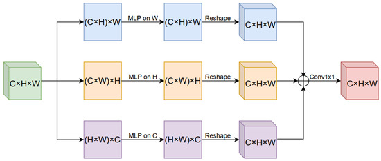
Figure 4.
The Spatial MLP (SMLP) module is composed of three branches, which mix the tokens along the row and column directions as well as the channel direction separately.
Let denote the input tensor of the SMLP module. In the horizontal path, the data tensor is reshaped into , and a linear layer with weights is applied to each row to mix information. Similar operations are performed in the vertical and channel paths, with weights and , respectively. Finally, the data tensors from the three paths are fused together to obtain a data tensor with the same dimensions as the input.
The number of parameters in an SMLP module can be calculated to be through computation. The , , and parameters are used for the three branches of the SMLP module, while the parameters are used for the fusion step. However, the number of parameters in the original MLP module is , where is the expansion ratio of the MLP layer, which is typically set to 4 in most cases. The decrease in computational complexity is also quite noticeable. The complexity of the SMLP module is
and the complexity of the MLP module is
If we use N to represent the product of H and W, it is easy to see that the computational complexity of the MLP module is , while the complexity of the SMLP module is . This, to some extent, reduces the computational complexity.
3.4. Spatial Self-Attention Module
Multi-head self-attention (MSA) is a variant of the attention mechanism that is commonly used in neural networks such as Transformer. It replaces the single attention head in the original self-attention mechanism with multiple heads, each of which can attend to a different information subspace in the input sequence, thereby improving the model’s accuracy and interpretability.
Overall, multi-head self-attention is an effective attention mechanism, but in practical use, we need to consider its impact on computational complexity and parameterization. On a satellite image, the number of pixels that belong to roads is relatively small compared to those that do not belong to roads, and roads are long-span, narrow, and continuously distributed. Therefore, using multi-head self-attention to calculate the spatial relationship information in the data tensor is unnecessary. In addition, most of the calculation in multi-head self-attention comes from invalid interference information in the feature space. Therefore, we designed a spatial self-attention (SSA) module, as shown in Figure 5, to replace the MSA module in Transformer to alleviate the two drawbacks of computational complexity and parameterization while ensuring attention to richer and more effective spatial information. The input tensor is passed through convolutions to obtain three branches of feature maps, which then undergo global average pooling (GAP) across three dimensions to obtain data tensors of sizes , , and . These tensors are then multiplied with each other to reconstruct a data tensor of the same dimension as the input tensor, which is finally fused with the input tensor and output.
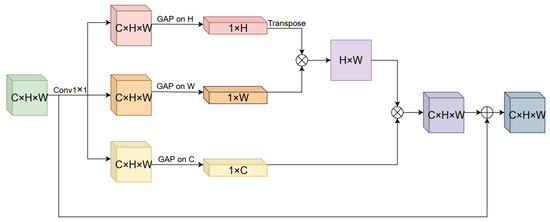
Figure 5.
The spatial self-attention (SSA) module captures long-range road feature information by performing global average pooling (GAP) across three different dimensions.
3.5. Loss Function
In the decoder part, we used dilated convolutions with dilation rates of 7, 5, 3, and 1 for upsampling, and finally, the feature map with a size of was outputted through a sigmoid function. The loss function is defined as follows:
where stands for binary cross entropy and stands for the Dice coefficient, which is defined as
where is a constant, N represents the number of elements in the slice, represents the ground truth for the given pixel at position i as either road or background, and represents the corresponding predicted probability of the segmentation branch.
4. Experimental Results and Analysis
4.1. Datasets
In our experiment, we chose two open-source remote sensing datasets for road extraction, namely the DeepGlobe dataset and the Massachusetts Road Dataset.
4.1.1. Massachusetts Dataset
The Massachusetts Road Dataset, established by [51], is an aerial imagery dataset that consists of urban and rural road data with complex and diverse features. It includes 1108 images for training, 14 images for validation, and 49 images for testing. The coverage area exceeds 2600 km2, and the size of each image is pixels, covering an area of 2.25 km2. As the training set contains some noisy images, we selected 733 images with minimal noise for training. Each image consists of pixels, and in the experiment, we divided the images into slices of size . The example image from the Massachusetts Roads Dataset is shown in Figure 6. The dataset is available at https://www.cs.toronto.edu/ṽmnih/data/ (accessed on 25 March 2024).
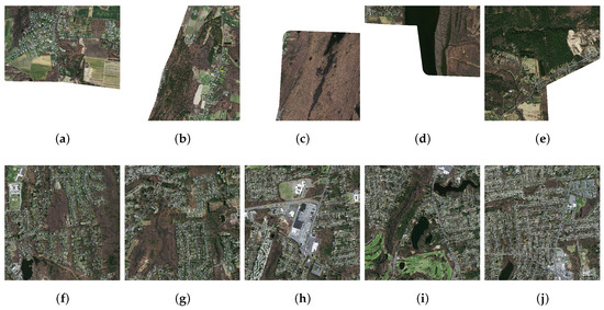
Figure 6.
The Massachusetts Road Dataset. Among them, the five images from (a–e) in the first row have significant noise, so we have removed these images from the dataset. However, the five images from (f–j) in the second row do not have noise, so we have chosen to keep these images.
4.1.2. DeepGlobe Dataset
The DeepGlobe dataset, established by [37], is an aerial imagery dataset covering regions in Thailand, Indonesia, and India. The dataset has high resolution and multispectral information, enabling the capture of fine details and features on the Earth’s surface. It is primarily used for tasks related to Earth observation, such as object classification and detection. The DeepGlobe dataset consists of 6226 images with a size of pixels and a resolution of 0.5 m. For experimentation purposes, the dataset is divided into 20,904 images with a size of pixels. This includes 18,676 images for training, 1557 images for validation, and 4671 images for testing. The example image from the DeepGlobe dataset is shown in Figure 7. The dataset is available at https://competitions.codalab.org/competitions/18467 (accessed on 25 March 2024).
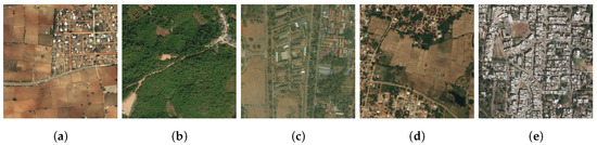
Figure 7.
The DeepGlobe dataset. The images from (a–e) are five randomly selected example images from the dataset. The images are sourced from Thailand, India, and Indonesia. The image scenes include various settings, such as cities, rural areas, barren lands, coastal regions, and tropical rainforests.
4.2. Evaluation Metrics
To fully evaluate all experimental methods, in our experiments, we used precision (P), recall (R), F1 score (F1), and Intersection over Union (IOU). These evaluation metrics are frequently used in binary semantic segmentation tasks and are calculated from TP, FP, TN, and FN. TP denotes correctly identified positive samples, FP denotes incorrectly identified positive samples, TN denotes correctly identified negative samples, and FN denotes incorrectly identified negative samples. These assessment metrics were calculated as follows:
4.3. Implementation Setting
In all models, the stochastic gradient descent (SGD) [52] optimizer is used for a batch size of eight. SGD is a commonly used optimization algorithm in machine learning, and is mainly used in the model training process. It is a variant of the gradient descent algorithm and is particularly suitable for processing large datasets. Compared with the traditional gradient descent method, it only randomly selects the gradient of one sample to update the model parameters in each iteration instead of calculating the gradients of all samples. The momentum decay coefficient and weight decay coefficient are set to 0.9 and , respectively. The initial learning rate is set to 0.01, and after each training iteration, the learning rate decays by 0.98 times the previous value. Our method is executed using the deep learning framework PyTorch, and the experiments are conducted on an NVIDIA RTX 3090 GPU with 24 GB memory. During the training process, we apply random horizontal rotation, random vertical rotation, and random scaling as data augmentations to improve the model’s generalization ability.
4.4. Experimental Results and Analysis
In order to demonstrate the effectiveness of the proposed SASwin Transformer architecture, we conducted experiments to evaluate the model using two publicly available road datasets. As a comparative evaluation, ten well-known methods were used as baselines, including FCN [6], UNet [7], ResUnet [36], SegNet [35], DeepLabV3 [8], LinkNet [53], D-LinkNet [9], CFPNet [54], TransUNet [48], SwinUNet [42], RoadExNet and RemainNet [55]. We compared all these methods in this experimental setting. Some multi-class segmentation methods were compared in the experiment. For example, TransUnet and SwinUNet use Softmax activation. However, road extraction is a second-class partitioning task using the Sigmoid activation function. Therefore, in the experiment, we replaced the Softmax activation function with Sigmoid. In order to better compare the performance of road extraction, we evaluated all methods using test samples from two publicly available datasets. For quantitative analysis, we used four evaluation metrics, precision (P), recall (R), F1 score (F1), and Intersection over Union (IoU), to assess all methods. To showcase the qualitative analysis results, we selected example images generated by some of the methods.
4.4.1. The Results of the Massachusetts Dataset
Table 1 displays the quantitative evaluation results of all methods in terms of P, R, F1, and IoU. In the table, the best performance is indicated in bold. Firstly, compared to FCN, UNet, ResUnet, SegNet, DeepLabV3, D-LinkNet, CFPNet, TransUNet, and SwinUnet, LinkNet achieves the best performance in terms of IoU. Secondly, our proposed SASwin Transformer significantly outperforms LinkNet. Compared to LinkNet, SASwin Transformer achieves the best performance in terms of R, F1, and IoU values, with an IoU of 65.04, which is 1.72 higher than that of LinkNet. This indicates that SASwin Transformer exhibits more foreground-awareness and robust performance, as its results are either the best or second best in all four metrics. The results demonstrate that the joint utilization of local and global features in our model encoder can reduce the number of misclassified pixels and improve the integrity and connectivity of road data.

Table 1.
The comparison results of the Massachusetts dataset are as follows. Higher values indicate better performance, and the best result is highlighted in bold. Among all the listed methods, our proposed approach achieved the highest IoU score.
From Figure 8, it can be seen that the proposed SASwin Transformer model achieves the best performance. For D-LinkNet, TransUNet, and SwinUnet, we observe that they miss road areas in many places, resulting in large false negatives (highlighted in red), especially at road intersections, corners, or regions obstructed by trees and buildings. Moreover, there are instances of disconnections in longer road segments. This can be attributed to the following reasons: (a) In the D-LinkNet architecture, D-LinkNet performs relatively well compared to CNN-based methods such as FCN, UNet, ResUnet, SegNet, DeepLabV3, LinkNet, and CFPNet. This is because D-LinkNet’s symmetric “U”-shaped structure effectively constructs segmentation maps from low-resolution feature maps and leverages multi-scale low-resolution feature maps to capture spatial context better. However, D-LinkNet solely focuses on local feature information and lacks the ability to establish long-range dependencies, which makes it challenging to detect obstructed regions caused by trees and buildings in the image. (b) In the SwinUnet architecture, SwinUnet is a pure Transformer-based encoder–decoder structure utilizing skip connections to fuse high-resolution features from different scales of the encoder to alleviate spatial information loss caused by downsampling. However, SwinUnet does not employ convolutions to fully extract local features, making it difficult to learn local semantic information. This results in the failure to detect road intersections and corners in the image. (c) In the TransUNet architecture, TransUNet employs three consecutive convolutions to extract three different-scale feature maps, which are then fed into a linear projection before being passed through a Transformer, and finally, a segmentation image is generated using skip connections and upsampling. Although TransUNet combines CNN and Transformer, it only performs global semantic information interaction in low-level feature maps, which is insufficient to establish long-range dependency relationships. In contrast, our proposed SASwin Transformer model effectively combines local and global semantic information at different feature scales. This is the reason why the SASwin Transformer method outperforms the other methods. The visual results align with the quantitative analysis results. Our model can better detect roads obstructed by trees, while other methods struggle to identify uncertain pixels. Additionally, our model is capable of generating more continuous results and reducing misclassifications of non-road pixels, resulting in fewer fragmented road segments and clearer results in the ground area.
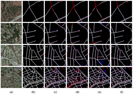
Figure 8.
The qualitative analysis results of different road segmentation methods on the Massachusetts dataset. False negatives are marked in red, and false positives are marked in blue. (a) Image. (b) Ground truth. (c) D-LinkNet. (d) TransUNet. (e) SwinUnet. (f) SASwin Transformer.
4.4.2. The Results of the DeepGlobe Dataset
Here, we report the road extraction results of the DeepGlobe dataset. Table 2 displays the quantitative results of our proposed SASwin Transformer compared to other methods on the DeepGlobe dataset. Our SASwin Transformer achieves an IoU score of 65.60, outperforming other methods and improving upon the second-best method, D-LinkNet, by 1.84. This can be attributed to the SMLP and SSA modules we designed, which both contribute to better capturing spatial features for road extraction.
Table 2.
The comparison results of the DeepGlobe dataset are as follows. Higher values indicate better performance, and the best result is highlighted in bold. Among all the listed methods, our proposed approach achieved the highest IoU score.
Figure 9 shows the example image results of four methods: D-LinkNet, TransUNet, SwinUnet, and SASwin Transformer. It can be observed that SwinUnet performs the worst, missing many fundamental road segments and resulting in some erroneous detections. Among the CNN-based encoder–decoder methods, D-LinkNet provides better results than SwinUnet and TransUNet. Among all the methods, the proposed SASwin Transformer generates the best results. This can be attributed to our effective fusion of local and global features, allowing for the generation of a powerful encoder for road extraction that captures rich spatial features more efficiently. Our proposed SASwin Transformer performs the best, consistent with our quantitative evaluation. The DeepGlobe road dataset consists mainly of remote sensing images from rural areas. It contains a large number of rural roads that exhibit various widths, indicating that a road may have different widths along its length. Additionally, a significant number of trees and shadows causes severe occlusions. The experimental results demonstrate the effectiveness of our SASwin Transformer in detecting rural roads. Combined with the results on the Massachusetts dataset, three out of the four quantitative evaluation metrics achieved the best performance on both datasets, indicating the robustness of our proposed method across different regions and road types.
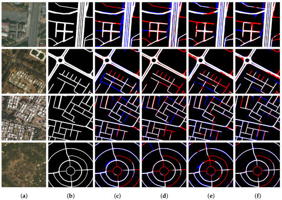
Figure 9.
The qualitative analysis results of different road segmentation methods on the DeepGlobe dataset. False negatives are marked in red, and false positives are marked in blue. (a) Image. (b) Ground truth. (c) D-LinkNet. (d) TransUNet. (e) SwinUnet. (f) SASwin Transformer.
4.5. Ablation Studies
Through ablation experiments and quantitative analysis, we can verify the effectiveness of the two modules proposed, namely SSA and SMLP. The experiments are typically conducted by gradually adding one module or a module combination to comprehensively evaluate the effectiveness of each module in the SASwin Transformer. Ablation experiments are performed on both the Massachusetts Road Dataset and the DeepGlobe dataset. General metrics are used to validate the overall prediction accuracy of the modules, while P, R, F1, and IoU are specifically used to validate road completeness after different modules are added. The training strategy and experimental environment used are the same as described in Section 4.3.
To better validate the effectiveness of each module, we replaced the SSA and SMLP modules in the SASwin Transformer with the MSA and MLP modules from the Swim Transformer as baselines. As shown in Table 3, SSA and SMLP further optimize the performance of the baseline. When SSA and SMLP are added individually to the baseline, the IoU increases by 0.77 and 0.32, respectively, compared to the baseline. When SSA and SMLP are combined and added to the baseline, the IoU improves by 2.14. As shown in Table 4, the combination of SSA and SMLP also improves the IoU scores. When SSA and SMLP are added individually to the baseline, the IoU increases by 0.83 and 1.00, respectively, compared to the baseline. When SSA and SMLP are combined and added to the baseline, the IoU improves by 1.57. This finding indicates that the combination of SSA and SMLP further enhances road extraction efficiency.
Table 3.
The ablation experiments were conducted on the Massachusetts dataset, with the best results highlighted in bold.
Table 4.
The ablation experiments were conducted on the DeepGlobe dataset, with the best results highlighted in bold.
As shown in Figure 10, the SASwin Transformer performs the best in the qualitative analysis, which is consistent with the results of the quantitative analysis. From the predicted sample images in the third row to the fifth row, it can be observed that some longer road segments are difficult to detect, resulting in fragmented road segments. Additionally, many road intersections and corners are also not recognized. The main reason for these issues is occlusion caused by dense vegetation and buildings. The combination of the SSA and SMLP modules can effectively alleviate such problems. The images demonstrate that after combining SSA and SMLP modules, the disconnected roads decrease and the missing road segments are inferred. Additionally, as shown in Table 3, we observe that adding SSA or SMLP individually can improve the precision (P) accuracy, while combining SSA and SMLP reduces the P value. This finding can be explained as follows: (a) adding a single module can improve network performance, (b) the combination of SSA and SMLP modules may introduce redundant information that affects the performance of different metrics, and (c) the Massachusetts Road Dataset does not annotate each pixel in the image, only marking the centerline information of the roads without road width information. Therefore, the issue of incorrect labeling may contribute to unstable predictions. Further research and continuous investigation are needed to address this problem.
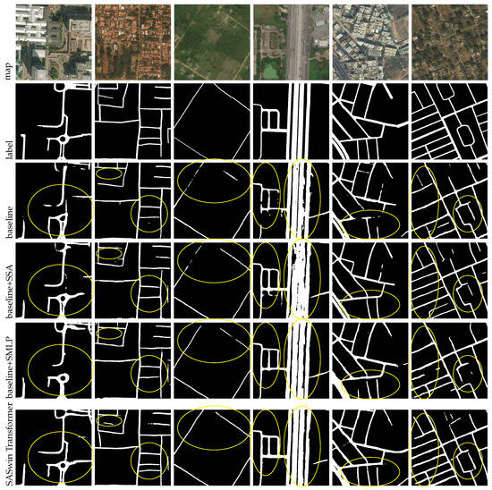
Figure 10.
The qualitative analysis results of the ablation experiments conducted on the DeepGlobe dataset are as follows, with differences highlighted in yellow circles. SSA improved the completeness of the results. SMLP improved the connectivity of the results. The proposed SASwin Transformer achieved the best performance.
To verify the efficiency of the proposed model, we compare it with the baseline. As shown in Table 5, the model parameter size is reduced from 84.94 M to 79.91 M, and the FLOPs are reduced from 130.61 G to 127.53 G. This clearly shows that SASwin Transformer is a more efficient modeling method.
Table 5.
The results of the comparison of the number of parameters and efficiency of the models.
4.6. Student’s T-Test
We conducted five Student’s t-test between the proposed method and the compared method. We used SASwin Transformer and other comparison methods to collect IoU results from five randomized experiments conducted on the Massachusetts and DeepGlobe datasets. Using the Student’s t-test method to calculate the p-value between our proposed method and the existing methods. When the p-value is greater than 0.05, there is no significant difference between the two models. When the p-value is less than 0.05, there is a significant difference in the results between the two models.
For the convenience of observing the differences in data, our experimental data are represented by scientific notation. As shown in Table 6, on two datasets, the p-values between the SASwin Transformer method and all comparative methods are less than 0.05, indicating that our SASwin Transformer method has a significant advantage over other methods. For example, on the Massachusetts dataset, the p-values between the SASwin Transformer method and the RoadExNet and RemainNet methods are and , respectively, both of which are less than 0.05, indicating a significant difference between the methods.
Table 6.
Student’s t-test results between SASwin Transformer and the compared methods.
5. Conclusions
This paper introduces the Spatial Attention Swin Transformer (SASwin Transformer) for road extraction. Our contribution is mainly to improve the Swin Transformer model to make it more suitable for extracting long-distance dependencies of road features. Compared with the original Swin Transformer model, this model has the advantages of higher precision, fewer parameters, and higher efficiency. The road has the characteristics of a large span and a narrow and continuous distribution. In order to extract road feature information more effectively, we replaced the MSA and MLP modules in Swin Transformer with SSA and SMLP modules to extract road feature information more adaptively. We also combine feature aggregation with ResNet to enhance multi-scale local spatial information, resulting in a stronger encoder to extract more efficient spatial features. The whole network structure follows the encoder–decoder architecture. In order to increase the acceptance domain of local features, we designed a bridge module for multi-scale feature learning. We tested our approach on the Massachusetts Road dataset and the DeepGlobe dataset. The experimental results show that the proposed method has better performance. Moreover, the proposed module can be easily integrated into any Swin Transformer-based architecture, indicating that our model has the potential for a wide range of applications.
In addition, the model proposed in this paper pays more attention to combining the CNN and Transformer from another perspective. Most of the existing methods use a serial approach to combine the CNN and Transformer. For example, Chen et al. proposed a TransUNet model that combines the features of Transformer and UNet. It first extracts features from the image using a CNN, obtains a feature map, and then converts the feature map and feeds it into the Transformer encoder module. Finally, it uses a decoder module similar to U-Net for on-layer sampling and jump connections, and finally generates segmentation results. Tao et al. proposed a Seg-Road model. In the encoder section, Seg-Road reduces the number of parameters by improving Transformer. In the decoder part, Seg-Road proposes a pixel connectivity structure (PCS) based on prior knowledge to improve road segmentation performance. Both the Seg-Road and TransUNet methods combine the CNN and Transformer in a way that resembles a “serial structure”. In our proposed model, a dual encoder method is used to extract local features through convolution in the CNN encoder part. In the Transformer encoder, Swin Transformer is improved to extract road characteristic information more adaptively. Our proposed model combines the CNN and Transformer in a way that resembles a “parallel architecture”. In general, our proposed model and methods like Seg-Road explore how to better combine CNN and Transformer from two different perspectives.
There is still some room for improvement in this paper. The process of inferring road could be extended to obtain vector outputs in practical applications of autonomous driving or path navigation, as claimed in the abstract. This would require applying knowledge of graph theory. Road node and edge information is generated during the inference process, and by combining this information, a final road topology can be generated. In addition, this paper can further investigate the sensitivity of the procedure to data quality. This is because studying the effect of procedures on data quality can help enhance the reliability and robustness of research results. Therefore, in future research, we will focus on this issue to further improve the research results in this area.
Author Contributions
Conception and editing, X.Z.; preparation and correction of the original manuscript, X.H. and W.C.; experimentation and analysis, Y.Z.; data curation, X.Y. and S.W. All authors have read and agreed to the published version of the manuscript.
Funding
This work was supported in part by the National Natural Science Foundation of China under grant Nos. 62062033 and 62301174, in part by the Natural Science Foundation of Jiangxi Province under grant No. 20232BAB202018, and in part by the Graduate Innovative Special Fund Projects of Jiangxi Province under grant No. YC2023-S530.
Data Availability Statement
No new data were created or analyzed in this study. Data sharing is not applicable to this article.
Conflicts of Interest
The authors declare no conflicts of interest. The funders had no role in the design of the study; in the collection, analyses, or interpretation of data; in the writing of the manuscript; or in the decision to publish the results.
References
- Li, Q.; Chen, L.; Li, M.; Shaw, S.L.; Nüchter, A. A Sensor-Fusion Drivable-Region and Lane-Detection System for Autonomous Vehicle Navigation in Challenging Road Scenarios. IEEE Trans. Veh. Technol. 2014, 63, 540–555. [Google Scholar] [CrossRef]
- Du, B.; Zhang, M.; Zhang, L.; Hu, R.; Tao, D. PLTD: Patch-Based Low-Rank Tensor Decomposition for Hyperspectral Images. IEEE Trans. Multimed. 2017, 19, 67–79. [Google Scholar] [CrossRef]
- Barzohar, M.; Cooper, D. Automatic finding of main roads in aerial images by using geometric-stochastic models and estimation. In Proceedings of the IEEE Conference on Computer Vision and Pattern Recognition, New York, NY, USA, 15–17 June 1993; pp. 459–464. [Google Scholar] [CrossRef]
- Laptev, I.; Mayer, H.; Lindeberg, T.; Eckstein, W.; Steger, C.; Baumgartner, A. Automatic extraction of roads from aerial images based on scale space and snakes. Mach. Vis. Appl. 2000, 12, 23–31. [Google Scholar] [CrossRef]
- Chai, D.; Förstner, W.; Lafarge, F. Recovering Line-Networks in Images by Junction-Point Processes. In Proceedings of the 2013 IEEE Conference on Computer Vision and Pattern Recognition, Portland, OR, USA, 23–28 June 2013; pp. 1894–1901. [Google Scholar] [CrossRef]
- Long, J.; Shelhamer, E.; Darrell, T. Fully convolutional networks for semantic segmentation. In Proceedings of the IEEE Conference on Computer Vision and Pattern Recognition, CVPR 2015, Boston, MA, USA, 7–12 June 2015; IEEE Computer Society: Washington, DC, USA, 2015; pp. 3431–3440. [Google Scholar] [CrossRef]
- Ronneberger, O.; Fischer, P.; Brox, T. U-Net: Convolutional Networks for Biomedical Image Segmentation. In Proceedings of the Medical Image Computing and Computer-Assisted Intervention-MICCAI 2015—18th International Conference, Munich, Germany, 5–9 October 2015; Proceedings, Part III; Lecture Notes in Computer Science. Navab, N., Hornegger, J., III, Wells, M.W., Frangi, A.F., Eds.; Springer: Berlin/Heidelberg, Germany, 2015; Volume 9351, pp. 234–241. [Google Scholar] [CrossRef]
- Chen, L.; Papandreou, G.; Schroff, F.; Adam, H. Rethinking Atrous Convolution for Semantic Image Segmentation. arXiv 2017, arXiv:1706.05587. [Google Scholar] [CrossRef]
- Zhou, L.; Zhang, C.; Wu, M. D-LinkNet: LinkNet With Pretrained Encoder and Dilated Convolution for High Resolution Satellite Imagery Road Extraction. In Proceedings of the 2018 IEEE Conference on Computer Vision and Pattern Recognition Workshops, CVPR Workshops 2018, Salt Lake City, UT, USA, 18–22 June 2018; Computer Vision Foundation/IEEE Computer Society: Washington, DC, USA, 2018; pp. 182–186. [Google Scholar] [CrossRef]
- Chen, L.C.; Papandreou, G.; Kokkinos, I.; Murphy, K.; Yuille, A.L. DeepLab: Semantic Image Segmentation with Deep Convolutional Nets, Atrous Convolution, and Fully Connected CRFs. IEEE Trans. Pattern Anal. Mach. Intell. 2018, 40, 834–848. [Google Scholar] [CrossRef] [PubMed]
- Cao, F.; Bao, Q. A Survey on Image Semantic Segmentation Methods with Convolutional Neural Network. In Proceedings of the 2020 International Conference on Communications, Information System and Computer Engineering (CISCE), Kuala Lumpur, Malaysia, 3–5 July 2020; pp. 458–462. [Google Scholar] [CrossRef]
- Yamashita, T.; Furukawa, H.; Fujiyoshi, H. Multiple Skip Connections of Dilated Convolution Network for Semantic Segmentation. In Proceedings of the 2018 25th IEEE International Conference on Image Processing (ICIP), Athens, Greece, 7–10 October 2018; pp. 1593–1597. [Google Scholar] [CrossRef]
- Mnih, V.; Hinton, G.E. Learning to Detect Roads in High-Resolution Aerial Images. In Proceedings of the Computer Vision-ECCV 2010-11th European Conference on Computer Vision, Heraklion, Crete, Greece, 5–11 September 2010; Proceedings, Part VI; Lecture Notes in Computer Science. Daniilidis, K., Maragos, P., Paragios, N., Eds.; Springer: Berlin/Heidelberg, Germany, 2010; Volume 6316, pp. 210–223. [Google Scholar] [CrossRef]
- Cheng, G.; Wang, Y.; Xu, S.; Wang, H.; Xiang, S.; Pan, C. Automatic Road Detection and Centerline Extraction via Cascaded End-to-End Convolutional Neural Network. IEEE Trans. Geosci. Remote Sens. 2017, 55, 3322–3337. [Google Scholar] [CrossRef]
- Panboonyuen, T.; Jitkajornwanich, K.; Lawawirojwong, S.; Srestasathiern, P.; Vateekul, P. Road Segmentation of Remotely-Sensed Images Using Deep Convolutional Neural Networks with Landscape Metrics and Conditional Random Fields. Remote Sens. 2017, 9, 680. [Google Scholar] [CrossRef]
- Ma, J.; Wu, L.; Tang, X.; Zhang, X.; Zhu, C.; Ma, J.; Jiao, L. Hyperspectral Image Classification Via Multi-Scale Encoder-Decoder Network. In Proceedings of the IGARSS 2020-2020 IEEE International Geoscience and Remote Sensing Symposium, Waikoloa, HI, USA, 26 September–2 October 2020; pp. 1283–1286. [Google Scholar] [CrossRef]
- Nakazawa, T.; Kulkarni, D.V. Anomaly Detection and Segmentation for Wafer Defect Patterns Using Deep Convolutional Encoder–Decoder Neural Network Architectures in Semiconductor Manufacturing. IEEE Trans. Semicond. Manuf. 2019, 32, 250–256. [Google Scholar] [CrossRef]
- Yan, F.; Yan, B.; Pei, M. Dual Transformer Encoder Model for Medical Image Classification. In Proceedings of the 2023 IEEE International Conference on Image Processing (ICIP), Kuala Lumpur, Malaysia, 8–11 October 2023; pp. 690–694. [Google Scholar] [CrossRef]
- Gai, L.; Chen, W.; Gao, R.; Chen, Y.W.; Qiao, X. Using Vision Transformers in 3-D Medical Image Classifications. In Proceedings of the 2022 IEEE International Conference on Image Processing (ICIP), Bordeaux, France, 16–19 October 2022; pp. 696–700. [Google Scholar] [CrossRef]
- Lu, D.; Xie, Q.; Gao, K.; Xu, L.; Li, J. 3DCTN: 3D Convolution-Transformer Network for Point Cloud Classification. IEEE Trans. Intell. Transp. Syst. 2022, 23, 24854–24865. [Google Scholar] [CrossRef]
- Meng, X.; Yang, Y.; Wang, L.; Wang, T.; Li, R.; Zhang, C. Class-Guided Swin Transformer for Semantic Segmentation of Remote Sensing Imagery. IEEE Geosci. Remote Sens. Lett. 2022, 19, 1–5. [Google Scholar] [CrossRef]
- Cheng, H.X.; Han, X.F.; Xiao, G.Q. TransRVNet: LiDAR Semantic Segmentation With Transformer. IEEE Trans. Intell. Transp. Syst. 2023, 24, 5895–5907. [Google Scholar] [CrossRef]
- Bastani, F.; He, S.; Abbar, S.; Alizadeh, M.; Balakrishnan, H.; Chawla, S.; Madden, S.; DeWitt, D. RoadTracer: Automatic Extraction of Road Networks from Aerial Images. In Proceedings of the 2018 IEEE/CVF Conference on Computer Vision and Pattern Recognition, Salt Lake City, UT, USA, 18–22 June 2018; pp. 4720–4728. [Google Scholar] [CrossRef]
- Tan, Y.; Gao, S.; Li, X.; Cheng, M.; Ren, B. VecRoad: Point-Based Iterative Graph Exploration for Road Graphs Extraction. In Proceedings of the 2020 IEEE/CVF Conference on Computer Vision and Pattern Recognition, CVPR 2020, Seattle, WA, USA, 13–19 June 2020; pp. 8907–8915. [Google Scholar] [CrossRef]
- He, S.; Bastani, F.; Jagwani, S.; Alizadeh, M.; Balakrishnan, H.; Chawla, S.; Elshrif, M.M.; Madden, S.; Sadeghi, M.A. Sat2Graph: Road Graph Extraction Through Graph-Tensor Encoding. In Proceedings of the Computer Vision-ECCV 2020-16th European Conference, Glasgow, UK, 23–28 August 2020; Proceedings, Part XXIV; Lecture Notes in Computer Science. Vedaldi, A., Bischof, H., Brox, T., Frahm, J., Eds.; Springer: Berlin/Heidelberg, Germany, 2020; Volume 12369, pp. 51–67. [Google Scholar] [CrossRef]
- Bahl, G.; Bahri, M.; Lafarge, F. Single-Shot End-to-end Road Graph Extraction. In Proceedings of the 2022 IEEE/CVF Conference on Computer Vision and Pattern Recognition Workshops (CVPRW), New Orleans, LA, USA, 18–24 June 2022; pp. 1402–1411. [Google Scholar]
- Xu, Z.; Liu, Y.; Gan, L.; Sun, Y.; Wu, X.; Liu, M.; Wang, L. RNGDet: Road Network Graph Detection by Transformer in Aerial Images. IEEE Trans. Geosci. Remote Sens. 2022, 60, 1–12. [Google Scholar] [CrossRef]
- Liu, Z.; Lin, Y.; Cao, Y.; Hu, H.; Wei, Y.; Zhang, Z.; Lin, S.; Guo, B. Swin Transformer: Hierarchical Vision Transformer using Shifted Windows. In Proceedings of the 2021 IEEE/CVF International Conference on Computer Vision (ICCV), Montreal, BC, Canada, 10–17 October 2021; pp. 9992–10002. [Google Scholar] [CrossRef]
- He, K.; Zhang, X.; Ren, S.; Sun, J. Deep Residual Learning for Image Recognition. In Proceedings of the 2016 IEEE Conference on Computer Vision and Pattern Recognition, CVPR 2016, Las Vegas, NV, USA, 27–30 June 2016; IEEE Computer Society: Washington, DC, USA, 2016; pp. 770–778. [Google Scholar] [CrossRef]
- He, Y.; Wang, H.; Zhang, B. Color based road detection in urban traffic scenes. In Proceedings of the 2003 IEEE International Conference on Intelligent Transportation Systems, Shanghai, China, 12–15 October 2003; Volume 1, pp. 730–735. [Google Scholar] [CrossRef]
- Zhang, Q.; Couloigner, I. Benefit of the angular texture signature for the separation of parking lots and roads on high resolution multi-spectral imagery. Pattern Recognit. Lett. 2006, 27, 937–946. [Google Scholar] [CrossRef]
- Wegner, J.D.; Montoya-Zegarra, J.A.; Schindler, K. A Higher-Order CRF Model for Road Network Extraction. In Proceedings of the 2013 IEEE Conference on Computer Vision and Pattern Recognition, Portland, OR, USA, 23–28 June 2013; IEEE Computer Society: Washington, DC, USA, 2013; pp. 1698–1705. [Google Scholar] [CrossRef]
- Song, M.; Civco, D.L. Road Extraction Using SVM and Image Segmentation. Photogramm. Eng. Remote Sens. 2004, 70, 1365–1371. [Google Scholar] [CrossRef]
- Krizhevsky, A.; Sutskever, I.; Hinton, G.E. ImageNet classification with deep convolutional neural networks. Commun. ACM 2012, 60, 84–90. [Google Scholar] [CrossRef]
- Badrinarayanan, V.; Kendall, A.; Cipolla, R. SegNet: A Deep Convolutional Encoder-Decoder Architecture for Image Segmentation. IEEE Trans. Pattern Anal. Mach. Intell. 2017, 39, 2481–2495. [Google Scholar] [CrossRef]
- Zhang, Z.; Liu, Q.; Wang, Y. Road Extraction by Deep Residual U-Net. IEEE Geosci. Remote Sens. Lett. 2018, 15, 749–753. [Google Scholar] [CrossRef]
- Demir, I.; Koperski, K.; Lindenbaum, D.; Pang, G.; Huang, J.; Basu, S.; Hughes, F.; Tuia, D.; Raskar, R. DeepGlobe 2018: A Challenge to Parse the Earth through Satellite Images. In Proceedings of the 2018 IEEE/CVF Conference on Computer Vision and Pattern Recognition Workshops (CVPRW), Salt Lake City, UT, USA, 18–22 June 2018; pp. 172–17209. [Google Scholar] [CrossRef]
- Wei, Y.; Zhang, K.; Ji, S. Simultaneous Road Surface and Centerline Extraction From Large-Scale Remote Sensing Images Using CNN-Based Segmentation and Tracing. IEEE Trans. Geosci. Remote Sens. 2020, 58, 8919–8931. [Google Scholar] [CrossRef]
- Cao, X.; Zhang, K.; Jiao, L. CSANet: Cross-Scale Axial Attention Network for Road Segmentation. Remote Sens. 2023, 15, 3. [Google Scholar] [CrossRef]
- Vaswani, A.; Shazeer, N.M.; Parmar, N.; Uszkoreit, J.; Jones, L.; Gomez, A.N.; Kaiser, L.; Polosukhin, I. Attention is All you Need. In Proceedings of the NIPS, Long Beach, CA, USA, 4–9 December 2017. [Google Scholar]
- Dosovitskiy, A.; Beyer, L.; Kolesnikov, A.; Weissenborn, D.; Zhai, X.; Unterthiner, T.; Dehghani, M.; Minderer, M.; Heigold, G.; Gelly, S.; et al. An Image is Worth 16x16 Words: Transformers for Image Recognition at Scale. In Proceedings of the 9th International Conference on Learning Representations, ICLR 2021, Virtual Event, 3–7 May 2021. [Google Scholar]
- Cao, H.; Wang, Y.; Chen, J.; Jiang, D.; Zhang, X.; Tian, Q.; Wang, M. Swin-Unet: Unet-Like Pure Transformer for Medical Image Segmentation. In Proceedings of the Computer Vision-ECCV 2022 Workshops, Tel Aviv, Israel, 23–27 October 2022; Proceedings, Part III; Lecture Notes in Computer Science. Karlinsky, L., Michaeli, T., Nishino, K., Eds.; Springer: Berlin/Heidelberg, Germany, 2022; Volume 13803, pp. 205–218. [Google Scholar] [CrossRef]
- Wang, W.; Xie, E.; Li, X.; Fan, D.; Song, K.; Liang, D.; Lu, T.; Luo, P.; Shao, L. Pyramid Vision Transformer: A Versatile Backbone for Dense Prediction without Convolutions. In Proceedings of the 2021 IEEE/CVF International Conference on Computer Vision, ICCV 2021, Montreal, QC, Canada, 10–17 October 2021; IEEE: Piscataway, NJ, USA, 2021; pp. 548–558. [Google Scholar] [CrossRef]
- Naseer, M.; Ranasinghe, K.; Khan, S.H.; Hayat, M.; Khan, F.S.; Yang, M.H. Intriguing Properties of Vision Transformers. Adv. Neural Inf. Process. Syst. 2021, 34, 23296–23308. [Google Scholar]
- Park, N.; Kim, S. How Do Vision Transformers Work? In Proceedings of the The Tenth International Conference on Learning Representations, ICLR 2022, Virtual Event, 25–29 April 2022. [Google Scholar]
- Li, Z.; Chen, H.; Jing, N.; Li, J. RemainNet: Explore Road Extraction from Remote Sensing Image Using Mask Image Modeling. Remote Sens. 2023, 15, 4215. [Google Scholar] [CrossRef]
- Gulati, A.; Qin, J.; Chiu, C.; Parmar, N.; Zhang, Y.; Yu, J.; Han, W.; Wang, S.; Zhang, Z.; Wu, Y.; et al. Conformer: Convolution-augmented Transformer for Speech Recognition. In Proceedings of the Interspeech 2020, 21st Annual Conference of the International Speech Communication Association, Shanghai, China, 25–29 October 2020; pp. 5036–5040. [Google Scholar] [CrossRef]
- Chen, J.; Lu, Y.; Yu, Q.; Luo, X.; Adeli, E.; Wang, Y.; Lu, L.; Yuille, A.L.; Zhou, Y. TransUNet: Transformers Make Strong Encoders for Medical Image Segmentation. arXiv 2021, arXiv:2102.04306. [Google Scholar]
- Luo, L.; Wang, J.X.; Chen, S.B.; Tang, J.; Luo, B. BDTNet: Road Extraction by Bi-Direction Transformer From Remote Sensing Images. IEEE Geosci. Remote Sens. Lett. 2022, 19, 2505605. [Google Scholar] [CrossRef]
- Tao, J.; Chen, Z.; Sun, Z.; Guo, H.; Leng, B.; Yu, Z.; Wang, Y.; He, Z.; Lei, X.; Yang, J. Seg-Road: A Segmentation Network for Road Extraction Based on Transformer and CNN with Connectivity Structures. Remote Sens. 2023, 15, 1602. [Google Scholar] [CrossRef]
- Mnih, V.; Hinton, G.E. Learning to Label Aerial Images from Noisy Data. In Proceedings of the the 29th International Conference on Machine Learning, ICML 2012, Edinburgh, UK, 26 June–1 July 2012. [Google Scholar]
- Ruder, S. An overview of gradient descent optimization algorithms. arXiv 2016, arXiv:1609.04747. [Google Scholar]
- Chaurasia, A.; Culurciello, E. LinkNet: Exploiting encoder representations for efficient semantic segmentation. In Proceedings of the 2017 IEEE Visual Communications and Image Processing, VCIP 2017, St. Petersburg, FL, USA, 10–13 December 2017; IEEE: Piscataway, NJ, USA, 2017; pp. 1–4. [Google Scholar] [CrossRef]
- Lou, A.; Loew, M. CFPNET: Channel-Wise Feature Pyramid For Real-Time Semantic Segmentation. In Proceedings of the 2021 IEEE International Conference on Image Processing (ICIP), Anchorage, AK, USA, 19–22 September 2021; pp. 1894–1898. [Google Scholar] [CrossRef]
- Chen, H.; Li, Z.; Wu, J.; Xiong, W.; Du, C. SemiRoadExNet: A semi-supervised network for road extraction from remote sensing imagery via adversarial learning. ISPRS J. Photogramm. Remote Sens. 2023, 198, 169–183. [Google Scholar] [CrossRef]
Disclaimer/Publisher’s Note: The statements, opinions and data contained in all publications are solely those of the individual author(s) and contributor(s) and not of MDPI and/or the editor(s). MDPI and/or the editor(s) disclaim responsibility for any injury to people or property resulting from any ideas, methods, instructions or products referred to in the content. |
© 2024 by the authors. Licensee MDPI, Basel, Switzerland. This article is an open access article distributed under the terms and conditions of the Creative Commons Attribution (CC BY) license (https://creativecommons.org/licenses/by/4.0/).