Abstract
Recently, with the remarkable advancements of deep learning in the field of image processing, convolutional neural networks (CNNs) have garnered widespread attention from researchers in the domain of hyperspectral image (HSI) classification. Moreover, due to the high performance demonstrated by the transformer architecture in classification tasks, there has been a proliferation of neural networks combining CNNs and transformers for HSI classification. However, the majority of the current methods focus on extracting spatial–spectral features from the HSI data of a single size for a pixel, overlooking the rich multi-scale feature information inherent to the data. To address this problem, we designed a novel transformer network with a CNN-enhanced cross-attention (TNCCA) mechanism for HSI classification. It is a dual-branch network that utilizes different scales of HSI input data to extract shallow spatial–spectral features using a multi-scale 3D and 2D hybrid convolutional neural network. After converting the feature maps into tokens, a series of 2D convolutions and dilated convolutions are employed to generate two sets of Q (queries), K (keys), and V (values) at different scales in a cross-attention module. This transformer with CNN-enhanced cross-attention explores multi-scale CNN-enhanced features and fuses them from both branches. Experimental evaluations conducted on three widely used hyperspectral image (HSI) datasets, under the constraint of limited sample size, demonstrate excellent classification performance of the proposed network.
1. Introduction
Hyperspectral imaging (HSI) has emerged as a powerful technique for remote sensing and the analysis of the Earth’s surface [1,2]. By capturing and analyzing a large number of narrow and contiguous spectral bands, HSI data provides rich and detailed information about the composition and properties of observed objects [3,4]. The ability to differentiate between different land cover types and detect subtle variations in materials has made HSI classification a crucial task in various fields, including agriculture [5], environmental monitoring [6], mineral exploration [7], and military reconnaissance [8]. HSI classification has become a hot research topic [9,10,11,12,13].
Currently, several HSI classification methods based on traditional machine learning algorithms have been proposed. These methods include Support Vector Machines (SVMs) [14,15] and Random Forest (RF) [16]. In addition, the k-Nearest Neighbors (k-NN) [17] algorithm is a non-parametric classification method that is based on the assumption of similar feature values. It assigns the class of an unlabeled pixel as the most frequent class among its k-nearest-neighboring pixels in the feature space. Linear Discriminant Analysis (LDA) [18] is a supervised dimensionality reduction and classification algorithm. It aims to find a linear transformation that maximizes the differences between different classes and minimizes the within-class scatter, resulting in discriminative features used for pixel classification. The Endmember Extraction and Classification Algorithm (EMAP) [19] is a comprehensive algorithm that combines endmember extraction and classification in hyperspectral image analysis. It involves extracting endmembers, which are pure spectral signatures, and using a linear mixing model to classify pixels based on their linear combinations of endmembers. EMAP enables the accurate characterization of materials present in hyperspectral data.
Traditional machine learning methods for hyperspectral classification have limitations in feature extraction, high-dimensional data, and modeling nonlinear relationships [20]. In contrast, deep learning offers advantages such as automatic feature learning, strong nonlinear modeling capabilities, compact data representation, and data augmentation for improved generalization [21]. These benefits make deep learning well-suited to handling high-dimensional, nonlinear, and complex hyperspectral data, leading to enhanced classification accuracy and robustness.
Due to the popularity of deep learning research, deep learning methods have also been applied to HSI classification tasks. Initially, researchers only used convolutional layers to solve classification tasks, such as 1D-CNN [22], 2D-CNN [23], and 3D-CNN [24]. However, more complex and deeper networks have been designed. He et al. [25] discovered that HSI differed significantly from 3D object images due to its combination of 2D spatial and 1D spectral features. Existing deep neural networks cannot be directly applied to HSI classification tasks. To address this issue, they proposed a Multiscale 3D Deep Convolutional Neural Network (M3D-CNN), which jointly learned both two-dimensional multiscale spatial features and one-dimensional spectral features from HSI data in an end-to-end manner. To achieve better classification performance by combining two types of convolutions, Roy et al. [26] effectively combined 3D-CNN with 2D-CNN. Zhu et al. [27] discovered the remarkable capabilities of Generative Adversarial Networks (GANs) in various applications. As a result, they explored the application of GANs in the field of HSI classification and designed a CNN for discriminating samples and another CNN for generating synthetic input samples. Their approach achieved superior classification accuracy compared to previous methods. Due to the sequential nature of hyperspectral pixels, Mou et al. [28] applied Recurrent Neural Networks (RNNs) to HSI classification tasks. Then, they proposed a novel RNN model that effectively analyzed HSI pixels as sequential data. Their research demonstrated the significant potential of RNNs in HSI classification tasks. Traditional CNN models can only capture fixed receptive fields for HSI, making it challenging to extract feature information with different object distributions. To address this issue, Wan et al. [29] applied Graph Convolutional Networks (GCNs) to HSI classification tasks. They designed a multi-scale dynamic GCN (MDGCN) that updated the graph dynamically during the convolution process, leveraging multiscale features in HSI.
With the introduction of attention mechanisms, Haut et al. [30] combined CNNs and Residual Networks (ResNets) with visual attention. Visual attention effectively assisted in identifying the most representative parts of the data. Experimental results demonstrated that deep attention models had a strong competitive advantage. Sun et al. [31] discovered that CNN-based methods, due to the presence of interfering pixels, weaken the discriminative power of spatial–spectral features. Hence, they proposed a Spectral–Spatial Attention Network (SSAN) that captured discriminative spatial–spectral features from attention areas in HSI. To leverage the diverse spatial–spectral features inherent in different regions of the training data, Hang et al. [32] proposed a novel attention-aided CNN. It consisted of two subnetworks responsible for extracting spatial and spectral features, respectively. Both subnetworks incorporated attention modules to assist in constructing a discriminative network. To mitigate the interference between spatial and spectral features during the extraction process, Ma et al. [33] designed a Double-Branch Multi-Attention mechanism network (DBMA). It employed two branches, each focusing on extracting spatial and spectral features, respectively, thereby reducing mutual interference. Subsequently, Zhu et al. [34] discovered that the equal treatment of all spectral bands using deep neural networks restricted feature learning and was not conducive to classification performance in HSI. Therefore, they proposed a Residual Spectral–Spatial Attention Network (RSSAN) to address this issue. The RSSAN took raw 3D cubes as input data and employed spectral attention and spatial attention to suppress irrelevant components and emphasize relevant components, achieving adaptive feature refinement.
Recently, with the introduction of Vision Transformer [35] into image processing, which originated from the transformer model in natural language processing, more and more efficient transformer structures have been designed [36]. To fully exploit the sequential properties inherent in the spectral feature of HSI, Hong et al. [37] proposed a new classification network called SpectralFormer. It can learn the spectral sequence information. Similarly, He et al. [38] also addressed this issue and designed a classification framework called Spatial–Spectral Transformer to capture the sequential spectral relationships in HSI. Due to the limited ability of CNN to capture deep semantic features, Sun et al. [39] discovered that transformer structures can effectively complement this drawback. They proposed a method called Spectral–Spatial Feature Tokenization Transformer (SSFTT). It combined CNNs and transformers to extract abundant spectral–spatial features. Mei et al. [40] found that the features extracted using the current transformer structures exhibited excessive discretization and, thus, proposed a Group-Aware Hierarchical Transformer (GAHT) based on group perception. This network used a hierarchical structure and achieved a significant improvement in classification performance. Fang et al. [41] introduced a Multi-Attention Joint Representation with Lightweight Transformer (MAR-LWFormer) for scenarios with extremely limited samples. They employed a three-branch structure to extract multi-scale features and demonstrated excellent classification performance. To utilize morphological features, Roy et al. [42] proposed a novel transformer (morphFormer) that combined morphological convolutional operations with attention mechanisms.
In the current research, most models are capable of effectively extracting spatial–spectral information from HSI. However, training on fixed-size sample cubes constrained the model’s ability to extract multi-scale features. Additionally, in practical applications, there is often a scarcity of labeled samples in HSI datasets [43]. Therefore, it is crucial to develop a network model that can adequately extract spatial–spectral features from HSI even in scenarios with limited samples.
The TNCCA model proposed by us offers the following three main contributions:
- Taking blocks of different sizes from HSI, we employ a mixed fusion multi-scale extraction shallow spatial–spectral feature module to process shallow features. This module primarily consists of two multi-scale convolutional neural networks designed for different-sized data. The network utilizes convolutional kernels of varying sizes to extract shallow feature information at different scales.
- An efficient transformer encoder was designed in which we apply 2D convolution and dilated convolution to tokens to obtain two sets of Q, K, and V with different scale information. This enables the transformer architecture with cross-attention to not only learn deeper feature information and promote the interaction of deep semantic information but also effectively fuse feature information of different sizes from the two branches.
- We designed an innovative dual-branch network specifically for classification tasks in small-sample scenarios. This network efficiently integrates a multi-scale CNN with a transformer encoder to fully exploit the multi-scale spatial–spectral features of HSI. We validated this network on three datasets, and the experimental results indicated that our proposed network was competitive compared to state-of-the-art methods.
2. Materials and Methods
In Figure 1, we illustrate an overview diagram of the proposed TNCCA model, which is an efficient dual-branch deep learning network for HSI classification. The network consists of the following sub-modules: the data preprocessing module for HSI, the shallow feature extraction module that utilizes different fusion methods to combine multi-scale spatial–spectral features, the module that converts the shallow features into tokens with different quantities assigned to different sizes, and the transformer module with CNN-enhanced cross-attention. Finally, there is the classifier head, which takes the input pixels and outputs the corresponding classification labels.
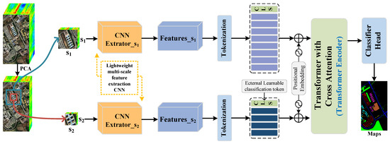
Figure 1.
Overview diagram of the proposed TNCCA model.
In summary, the TNCCA model consists of the following five components: HSI data preprocessing, a dual-branch multi-scale shallow feature extraction module, a feature-maps-to-tokens conversion module, a transformer with a CNN-enhanced cross-attention module, and a classifier head.
2.1. HSI Data Preprocessing
The processing of the original HSI () is described in this section, where a and b represent different spatial sizes, and l represents the spectral dimension. Due to the typically large number of spectral dimensions in HSI, it increases computational complexity and consumes significant computational resources. Therefore, we use the PCA operation to solve this problem by reducing the dimensionality of the original image from l to r.
To obtain information at different scales, we extract two square patches of different sizes, and (), centered at each pixel. We combine these two variables into a dataset and feed it into the network together. Finally, the set of data generated via each pixel is placed into a collection, A, and the training and test sets are randomly partitioned from A based on the sampling rate. Each group of training and testing data contains the corresponding ground truth labels. The labels, denoted as , are obtained from the set of ground truth labels.
2.2. Dual-Branch Multi-Scale Shallow Feature Extraction Module
As shown in Figure 2, a group of cubes, denoted as and , with different sizes are fed into the network. Firstly, they pass through a 3D convolutional layer. In the first branch, a larger-sized cube is processed, and 8 convolutional kernels are allocated. The size of each kernel is (). In the second branch, a cube with smaller dimensions is processed, and 4 convolutional kernels are allocated. The size of each kernel is (). To maintain the original size of the cubes, padding is applied. The above process can be represented in the following equation:
where Conv3D and Conv2D represent 3D convolutional layers and 2D convolutional layers with different kernel sizes, respectively.
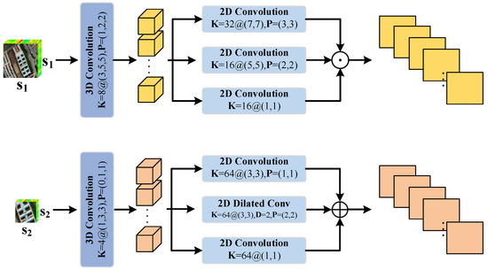
Figure 2.
Dual-branch multi-scale shallow feature extraction module.
After passing through a 3D convolutional layer, we extract shallow spatial features at different scales using multi-scale 2D convolutional layers. Similarly, we use different numbers of convolutional kernels and different kernel sizes in different branches. In the first branch, we use 32 2D convolutional kernels of size (), 16 kernels of size (), and 16 kernels of size (). The information from these three different scales is fused through the Concatenation operation. In the second branch, smaller kernel sizes are used to extract shallow spatial features. Specifically, we use 64 2D convolutional kernels of size (), 64 2D dilated convolutional kernels with a dilation rate of 2 and size (), and 64 2D convolutional kernels of size (). The information from these three different scales is fused through element-wise addition.
Finally, we obtain two sets of 2D features, and , respectively. This process can be represented in the following equations:
2.3. Feature-Maps-to-Tokens Conversion Module
After obtaining the multi-scale 2D feature information from the dual-branch shallow feature extraction module, in order to better adapt to the structure of the Transformer, these features need to be tokenized.
The flattened feature maps are denoted as and , respectively. These two variables can be represented in the following equation:
where (·) is a transpose function. Next, is multiplied by a learnable weight matrix using a 1 × 1 operation, and similarly, is multiplied by a learnable weight matrix using a 1 × 1 operation. We use weight matrices of different shapes to achieve the purpose of assigning a different number of tokens. Then, the feature maps are transformed into feature tokens multiplied by themselves. The above process can be achieved using the following equation:
To accomplish the classification task, we also embed a learnable classification token consisting of all zeros. Then, to preserve the original positional information, positional information is embedded into the tokens. The tokens of the two branches can be obtained from the following equation:
2.4. Transformer with CNN-Enhanced Cross-Attention Module
The transformer possesses powerful feature-information-mining capabilities, as it can capture long-range dependencies and acquire global contextual information. To further explore the deep feature information contained in the data and fully integrate the multi-scale feature information extracted via the two branches, we embed a cross-attention in the transformer structure.
As shown in Figure 3, We utilize different convolutional layers to obtain the attention mechanism’s Q, K, and V tensors from one of the outputs obtained from the previous module. Firstly, we apply a 2D convolutional layer with kernel sizes of () and padding of 1 to obtain . Next, a 2D convolutional layer with kernel sizes of () and padding of 2 is used to obtain . Finally, we employ a dilated convolutional layer with kernel sizes of (), padding of 2, and a dilation rate of 2 to obtain .
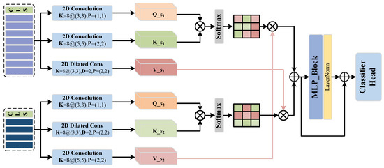
Figure 3.
Transformer with CNN-enhanced cross-attention module.
Next, we apply similar multi-scale convolutions to another output, , to obtain , , and . Firstly, we use a 2D convolutional layer with a kernel size of () and padding of 1 to obtain . Then, we employ a dilated convolutional layer with a kernel size of (), padding of 2, and a dilation rate of 2 to obtain . Finally, we utilize a 2D convolutional layer with a kernel size of () and padding of 2 to obtain . Once we have obtained these tensors, we perform element-wise multiplication among them to obtain deep features and that have undergone the attention mechanism. The process can be represented in the following formula:
where is the dimension of , and is the dimension of . We obtain the deep features from two branches and sum them pixel-wise. Then, we pass the summed features through a multi-layer perceptron block using a residual structure to obtain the final deep feature, . This can be obtained using the following equation:
where is the multi-layer perceptron, and is the abbreviation for layer normalization. The MLP mainly includes two linear layers, with the addition of the Gaussian Error Linear Unit (GELU) activation function in between.
2.5. Classifier Head
We extract the learnable classification token, , from the output tokens, , of the transformer encoder. Then, we pass it through a linear layer to obtain a one-dimensional vector, denoted as , where c represents the number of classes. The softmax function is used to ensure that the total activation of each output unit is 1. By selecting the corresponding maximum value, we obtain the class label for that pixel. The entire process can be represented in the following equation:
The complete procedure of the TNCCA method, as proposed, is outlined in Algorithm 1.
| Algorithm 1 Multi-scale Feature Transformer with CNN-Enhanced Cross-Attention Model |
Input: Input HSI data and ground truth labels ; the original data are reduced in spectral dimension to r = 30 using PCA operation. A set of small cubes with sizes = 13 and = 7 is then extracted. Subsequently, the training set of the model is randomly sampled at a sampling rate of 1%. Output: Predicted labels for the test dataset.
|

Table 1.
Explanation of the division of training samples and test samples in the Houston2013 dataset, the Trento dataset, and the Pavia University dataset.
Table 1.
Explanation of the division of training samples and test samples in the Houston2013 dataset, the Trento dataset, and the Pavia University dataset.
| NO. | Houston2013 Dataset | Trento Dataset | Pavia University Dataset | ||||||
|---|---|---|---|---|---|---|---|---|---|
| Class | Training (). | Test. | Class | Training (). | Test. | Class | Training (). | Test. | |
| #1 | Healthy Grass | 13 | 1238 | Apple Trees | 40 | 3994 | Asphalt | 66 | 6565 |
| #2 | Stressed Grass | 13 | 1241 | Buildings | 29 | 2874 | Meadows | 186 | 18,463 |
| #3 | Synthetic Grass | 7 | 690 | Ground | 5 | 474 | Gravel | 21 | 2078 |
| #4 | Tree | 12 | 1232 | Woods | 91 | 9032 | Trees | 31 | 3033 |
| #5 | Soil | 12 | 1230 | Vineyard | 105 | 10,396 | Metal Sheets | 13 | 1332 |
| #6 | Water | 3 | 322 | Roads | 31 | 3143 | Bare Soil | 50 | 4979 |
| #7 | Residential | 13 | 1255 | Bitumen | 13 | 1317 | |||
| #8 | Commercial | 12 | 1232 | Bricks | 37 | 3645 | |||
| #9 | Road | 13 | 1239 | Shadows | 9 | 938 | |||
| #10 | Highway | 12 | 1215 | ||||||
| #11 | Railway | 12 | 1223 | ||||||
| #12 | Parking Lot 1 | 12 | 1221 | ||||||
| #13 | Parking Lot 2 | 5 | 464 | ||||||
| #14 | Tennis Court | 4 | 424 | ||||||
| #15 | Running Track | 7 | 653 | ||||||
| Total | 150 | 14,879 | Total | 301 | 29,913 | Total | 426 | 42,350 | |
3. Results
3.1. Data Description
The proposed TNCCA model was tested on three widely used datasets. Below, we introduce these three datasets one by one.
Houston2013 dataset: The Houston2013 dataset was jointly provided by the research group at the University of Houston and the National Mapping Center of the United States. It contained a wide range of categories and has been widely used by researchers. The dataset consisted of 144 bands and contained classified pixels. There were 15 different classification categories. Figure 4 displayed the pseudocolored image and ground truth map of the Houston2013 dataset.
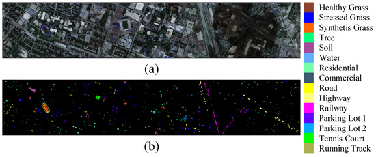
Figure 4.
Presentation of the Houston2013 dataset. (a) Pseudo-color image composed of three spectral bands. (b) Ground truth map.
Trento dataset: The Trento dataset was captured in the southern region of Trento, Italy. It was an HSI obtained using the Airborne lmaging Spectrometer for Application (AISA) Eagle sensor. The dataset consisted of 63 spectral bands and had dimensions of pixels for classification. It included six different categories of ground objects. Figure 5a,b respectively display the pseudocolored image and ground truth map.

Figure 5.
Presentation of the Trento dataset. (a) Pseudo-color image composed of three spectral bands. (b) Ground truth map.
Pavia University dataset: The Pavia University dataset was a collection of HSI taken in 2001, specifically at Pavia University in Italy. The dataset was an HSI obtained using a Reflective Optics System Imaging Spectrometer (ROSIS) sensor. The image comprised 115 bands and had dimensions of classified pixels. There were a total of nine land cover classification categories. To reduce the interference of noise, we removed 12 bands that contained noise. Figure 6 displays the pseudocolored image and ground truth map of the dataset.
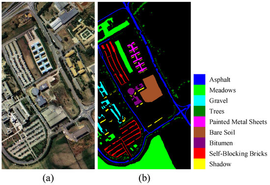
Figure 6.
Presentation of the Pavia University dataset. (a) Pseudo-color image composed of three spectral bands. (b) Ground truth map.
We present the division of training and test samples for the three datasets in Table 1, which includes the specific data for each category. For each category, we used of the total number of samples as the training set.
3.2. Parameter Analysis
In the model we proposed, there was a set of hyperparameters, such as batch size, the size of the first cubic patch, and the size of the second cubic patch. We conducted experimental analysis on these parameters to ensure that their values were optimal. The analysis results are shown in Figure 7, Figure 8 and Figure 9.
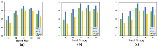
Figure 7.
Validation of the optimal hyperparameters with different classification metrics for the Houston2013 dataset. (a) Batch size. (b) Size of the cubic patch in the first branch. (c) Size of the cubic patch in the second branch.
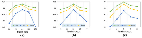
Figure 8.
Validation of the optimal hyperparameters with different classification metrics for the Trento dataset. (a) Batch size. (b) Size of the cubic patch in the first branch. (c) Size of the cubic patch in the second branch.
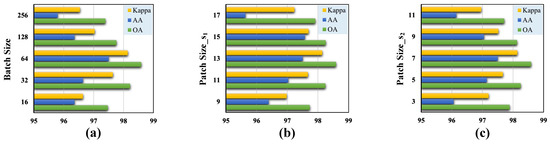
Figure 9.
Validation of the optimal hyperparameters with different classification metrics for the Pavia University dataset. (a) Batch size. (b) Size of the cubic patch in the first branch. (c) Size of the cubic patch in the second branch.
(1) Batch Size: Due to our observation that the performance of the transformer architecture was highly sensitive to the batch size, different sizes resulted in varying classification performance. We set the batch size to the following candidate values: . Additionally, we experimentally determined the batch size that yielded the best performance for our proposed model.
(2) Patch Size: Since the cubic patch served as the input to the model, selecting a patch size that was too small could limit the model’s receptive field, while choosing a size that was too large could result in excessive data volume and increased computational complexity. Our proposed TNCCA selected two different sizes of cubic patches to extract multi-scale features, for which the size of the cubic patch in the first branch was slightly larger than that in the second branch. These two cubic patches served as inputs to the model, and their sizes significantly impacted the classification accuracy. Therefore, we conducted experiments on these two hyperparameters.
We first selected the parameter for the first branch from the set , and the experimental results showed that the model achieved the best classification performance when its value was 13. Then, for the second branch, we selected the parameter from the set . From Figure 7, Figure 8 and Figure 9, it can be observed that the model achieved the highest classification metrics when its value was 7.
3.3. Classification Results and Analysis
We explored eight advanced classification models, and in this section, we describe the conducted experiments and analyze them to compare the classification performance of our proposed model with these models. They comprised SVM [14], 1D-CNN [22], 3D-CNN [24], M3D-CNN [25], 3D-DLA [44], Hybrid [26], SSFTT [39], and morphFormer [42]. To maintain the original performance of the comparative models, we used the training strategies described in their respective papers. The number of training and testing samples for each model was the same as the numbers listed in Table 1, and random sampling was employed. If you wish to reproduce our experiments, you can download the code from the following link: https://github.com/cupid6868/TNCCA.git (accessed on 25 March 2024).
(1) Quantitative results and analysis: We present the results in Table 2, Table 3 and Table 4, where we demonstrate the superior performance of our proposed model. We highlight the best results for each metric. We conducted experiments on three datasets: the Houston2013 dataset, the Trento dataset, and the Pavia University dataset. The comparative classification metrics included overall accuracy (OA), average accuracy (AA), the Kappa coefficient (), and class-wise accuracy. The data in the tables clearly indicate that our proposed TNCCA outperformed the other seven models on the experimental datasets. Let us take the Houston2013 dataset as an example. The proposed TNCCA exhibited the best classification performance for classes such as ‘Synthetic Grass’, ‘Soil’, ’Water’, ‘Commercial’, ‘Parking Lot 2’, ‘Tennis Court’, and ‘Running Track’. Additionally, for classes like ‘Healthy Grass’, ‘Stressed Grass’, and ‘Parking Lot 1’, although our model’s performance was not the best, it still ranked among that of the top methods. In contrast, SVM and 1D-CNN showed extremely low classification performance for certain classes. This clearly demonstrated that, in the context of small sample sizes, our proposed model effectively utilized multi-scale feature information and fully exploited the spatial–spectral characteristics in HSI.
Table 2.
Comparison of classification performance using the Houston2013 dataset with different methods (The optimal results are shown in bold, and the names of land-covers are shown in italics).
Table 3.
Comparison of classification performance using the Trento dataset with different methods (The optimal results are shown in bold, and the names of land-covers are shown in italics).
Table 4.
Comparison of classification performance using the Pavia University dataset with different methods (The optimal results are shown in bold, and the names of land-covers are shown in italics).
(2) Visual evaluation and analysis: We present the aforementioned experimental results in the form of classification maps, shown in Figure 10, Figure 11 and Figure 12. By comparing the spatial contours of the classification maps with the noise contained in the images, we can clearly observe the superior classification performance of the proposed TNCCA compared to other models.
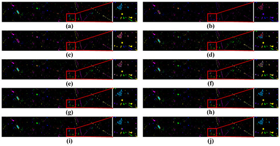
Figure 10.
Visualization of classification results using different classification methods with the Houston2013 dataset. (a) Ground truth map, (b) SVM (OA = 33.24%), (c) 1D-CNN (OA = 33.63%), (d) 3D-CNN (OA = 48.39%), (e) M3D-CNN (OA = 68.44%), (f) 3D-DLA (OA = 70.49%), (g) hybrid (OA = 77.29%), (h) SSFTT (OA = 87.85%), (i) morphFormer (OA = 87.17%), and (j) the proposed method (OA = 90.72%).
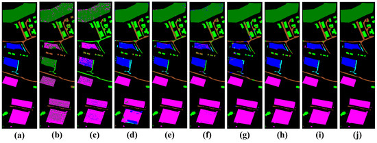
Figure 11.
Visualization of classification results using different classification methods with the Trento dataset. (a) Ground truth map, (b) SVM (OA = 67.74%), (c) 1D-CNN (OA = 70.75%), (d) 3D-CNN (OA = 91.27%), (e) M3D-CNN (OA = 94.91%), (f) 3D-DLA (OA = 92.91%), (g) hybrid (OA = 92.21%), (h) SSFTT (OA = 97.88%), (i) morphFormer (OA = 98.20%), and (j) the proposed method (OA = 98.98%).
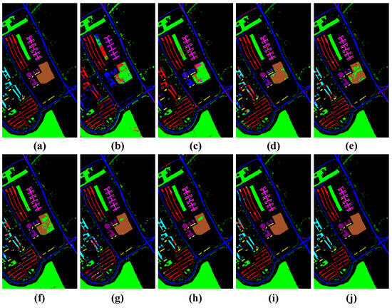
Figure 12.
Visualization of classification results using different classification methods with the Pavia University dataset. (a) Ground truth map, (b) SVM (OA = 33.24%), (c) 1D-CNN (OA = 33.63%), (d) 3D-CNN (OA = 48.39%), (e) M3D-CNN (OA = 68.44%), (f) 3D-DLA (OA = 70.49%), (g) hybrid (OA = 77.29%), (h) SSFTT (OA = 87.85%), (i) morphFormer (OA = 87.17%), and (j) the proposed method (OA = 90.72%).
In the classification maps, it is obvious that the classification map of TNCCA exhibited the clearest spatial contours and contained the least amount of noise. Conversely, the classification maps of the other models showed more instances of misclassifications and interfering noise. Let us take the classification map of the Houston2013 dataset as an example. The classification map of our proposed model closely resembles the ground truth map. On the other hand, the classification maps of SVM, 1D-CNN, 3D-CNN, M3D-CNN, and 3D-DLA exhibited more misclassifications and noise. In the zoomed-in window, we can clearly observe the high classification performance of our proposed model for classes such as ‘Parking Lot 2’, ‘Road’, and ‘Synthetic Grass’.
In conclusion, our proposed model outperformed the compared models and demonstrated the best classification performance. It highlighted the model’s capability of extracting features effectively in small sample scenarios.
3.4. Analysis of Inference Speed
To demonstrate the inference speed of our proposed model, TNCCA, we present the training time and testing time of the model with different datasets in Table 5. The data show that our training speed is fast, as the model can complete 500 epochs in a very short period. To facilitate the observation of model performance during the training process, we adopted a training strategy of conducting a test after each epoch. This resulted in a significantly longer testing time compared to the training time. Additionally, we employed dynamic learning rates to accelerate the convergence speed.
Table 5.
The inference speed of TNCCA on different datasets (epoch = 500).
Among the three tested datasets, the Pavia University dataset, which had larger spatial dimensions and higher spectral dimensions, took the longest time, with 1.26 min for training and only 0.153 s per epoch. The training times for the other datasets were shorter. From this table, it is easy to conclude that our proposed model not only achieved high classification accuracy but also trained at a fast speed, demonstrating high efficiency.
3.5. Ablation Analysis
To validate the effectiveness of each module in our proposed model, we conducted ablation experiments on the four modules using the Houston2013 dataset. These four modules comprised a 3D convolutional layer (3D-Conv), a multi-scale 2D convolutional module (Ms2D-Conv), a feature map tokenization module (Tokenizer), and a transformer encoder module (TE). We evaluated their performance in terms of OA, AA, and by considering five different combinations of these modules. The results are listed in Table 6.
Table 6.
Conducting ablation experiments on different modules (using the Houston2013 dataset).
Specifically, we first kept only the 3D convolutional layer, and it was evident that the performance was extremely poor. In the next step, we removed the transformer encoder with the CNN-enhanced cross-attention mechanism, which was one of the main innovations of this paper. The results showed a significant decrease in classification performance. The OA, AA, and values of the model decreased by , , and , respectively, compared to TNCCA. Next, we removed the 3D convolutional layer and replaced the multi-scale 2D convolutional module with a regular 2D convolutional layer. In this configuration, the model’s OA decreased by , and its AA decreased by , compared to TNCCA. Then, we removed the 3D convolutional layer, which resulted in the loss of rich spectral information in the HSI. We observed that the model’s OA decreased by , and its AA decreased by , compared to TNCCA. Finally, we replaced only the multi-scale 2D convolutional module with a regular 2D convolutional layer. In this case, the model’s OA decreased by , and its AA decreased by , compared to TNCCA. This clearly demonstrated the positive contributions of these four modules in enhancing the accuracy of network classification.
4. Conclusions
The paper has introduced a novel dual-branch deep learning classification model that effectively captures spatial–spectral feature information from HSI and achieves high classification performance in small sample scenarios. The two branches of the model utilize cubic patches of different sizes as inputs to fully exploit the limited samples and extract features at different scales. First, we employed a 3D convolutional layer and a multi-scale 2D convolutional module to extract shallow-level features. Then, the obtained feature maps were transformed into tokens, assigning a larger number of tokens to the larger cubic patches. Next, we utilized a transformer with CNN-enhanced cross-attention to delve into the deep-level feature information and fuse the different-scale information from the two branches. Finally, through extensive experiments, we demonstrated that the proposed TNCCA model exhibits superior classification performance.
In our future work, we aim to explore the rich multi-scale spatial–spectral features in HSI from different perspectives to improve classification accuracy. However, as the classification accuracy improves, there is an increasing demand for lightweight operations and reducing the computational complexity of the models. We will utilize more novel lightweight operations to design more efficient classification models.
Author Contributions
Methodology, X.W. and B.L.; conceptualization, X.W. and L.S.; software, X.W. and L.S.; validation, X.W. and C.L.; investigation, B.L. and X.W.; writing—original draft preparation, X.W.; writing—review and editing, B.L. and L.S.; visualization, C.L. and X.W.; All authors have read and agreed to the published version of the manuscript.
Funding
This research was funded by the Jiangsu key R&D plan, no. BE2022161.
Data Availability Statement
The data presented in this study are available in the article.
Acknowledgments
The authors thank the anonymous reviewers and the editors for their insightful comments and helpful suggestions that helped improve the quality of our manuscript.
Conflicts of Interest
The authors declare no conflicts of interest.
Abbreviations
The following abbreviations are used in this manuscript:
| HSI | Hyperspectral image |
| RF | Random Forest |
| SVM | Support Vector Machine |
| LDA | Linear Discriminant Analysis |
| PCA | Principal Component Analysis |
| CNN | Convolutional Neural Network |
| GAN | Generative Adversarial Network |
| GCN | Graph Convolutional Network |
| RNN | Recurrent Neural Network |
| ResNet | Residual Network |
| TE | Transformer encoder |
| Q | Queries |
| K | Keys |
| V | Values |
| MLP | Multi-layer perceptron |
| LN | Normalization layers |
References
- He, C.; Cao, Q.; Xu, Y.; Sun, L.; Wu, Z.; Wei, Z. Weighted Order-p Tensor Nuclear Norm Minimization and Its Application to Hyperspectral Image Mixed Denoising. IEEE Geosci. Remote Sens. Lett. 2023, 20, 5510505. [Google Scholar] [CrossRef]
- Sun, L.; Wang, Q.; Chen, Y.; Zheng, Y.; Wu, Z.; Fu, L.; Jeon, B. CRNet: Channel-Enhanced Remodeling-Based Network for Salient Object Detection in Optical Remote Sensing Images. IEEE Trans. Geosci. Remote Sens. 2023, 61, 5618314. [Google Scholar] [CrossRef]
- Gao, H.; Zhang, Y.; Chen, Z.; Xu, S.; Hong, D.; Zhang, B. A Multidepth and Multibranch Network for Hyperspectral Target Detection Based on Band Selection. IEEE Trans. Geosci. Remote Sens. 2023, 61, 5506818. [Google Scholar] [CrossRef]
- Gao, H.; Zhang, Y.; Chen, Z.; Xu, F.; Hong, D.; Zhang, B. Hyperspectral Target Detection via Spectral Aggregation and Separation Network With Target Band Random Mask. IEEE Trans. Geosci. Remote Sens. 2023, 61, 5515516. [Google Scholar] [CrossRef]
- Gevaert, C.M.; Suomalainen, J.; Tang, J.; Kooistra, L. Generation of Spectral–Temporal Response Surfaces by Combining Multispectral Satellite and Hyperspectral UAV Imagery for Precision Agriculture Applications. IEEE J. Sel. Top. Appl. Earth Obs. Remote Sens. 2015, 8, 3140–3146. [Google Scholar] [CrossRef]
- Gong, P.; Li, Z.; Huang, H.; Sun, G.; Wang, L. ICESat GLAS Data for Urban Environment Monitoring. IEEE Trans. Geosci. Remote Sens. 2011, 49, 1158–1172. [Google Scholar] [CrossRef]
- Wang, J.; Zhang, L.; Tong, Q.; Sun, X. The Spectral Crust project—Research on new mineral exploration technology. In Proceedings of the 2012 4th Workshop on Hyperspectral Image and Signal Processing: Evolution in Remote Sensing (WHISPERS), Shanghai, China, 4–7 June 2012; pp. 1–4. [Google Scholar] [CrossRef]
- Ardouin, J.P.; Levesque, J.; Rea, T.A. A demonstration of hyperspectral image exploitation for military applications. In Proceedings of the 2007 10th International Conference on Information Fusion, Québec, QC, Canada, 9–12 July 2007; pp. 1–8. [Google Scholar] [CrossRef]
- Su, Y.; Gao, L.; Jiang, M.; Plaza, A.; Sun, X.; Zhang, B. NSCKL: Normalized Spectral Clustering With Kernel-Based Learning for Semisupervised Hyperspectral Image Classification. IEEE Trans. Cybern. 2023, 53, 6649–6662. [Google Scholar] [CrossRef] [PubMed]
- Su, Y.; Chen, J.; Gao, L.; Plaza, A.; Jiang, M.; Xu, X.; Sun, X.; Li, P. ACGT-Net: Adaptive Cuckoo Refinement-Based Graph Transfer Network for Hyperspectral Image Classification. IEEE Trans. Geosci. Remote Sens. 2023, 61, 5521314. [Google Scholar] [CrossRef]
- Yu, H.; Gao, L.; Liao, W.; Zhang, B.; Zhuang, L.; Song, M.; Chanussot, J. Global Spatial and Local Spectral Similarity-Based Manifold Learning Group Sparse Representation for Hyperspectral Imagery Classification. IEEE Trans. Geosci. Remote Sens. 2020, 58, 3043–3056. [Google Scholar] [CrossRef]
- Gao, H.; Yang, Y.; Li, C.; Gao, L.; Zhang, B. Multiscale Residual Network With Mixed Depthwise Convolution for Hyperspectral Image Classification. IEEE Trans. Geosci. Remote Sens. 2021, 59, 3396–3408. [Google Scholar] [CrossRef]
- Yan, L.; Fan, B.; Liu, H.; Huo, C.; Xiang, S.; Pan, C. Triplet Adversarial Domain Adaptation for Pixel-Level Classification of VHR Remote Sensing Images. IEEE Trans. Geosci. Remote Sens. 2020, 58, 3558–3573. [Google Scholar] [CrossRef]
- Melgani, F.; Bruzzone, L. Classification of hyperspectral remote sensing images with support vector machines. IEEE Trans. Geosci. Remote Sens. 2004, 42, 1778–1790. [Google Scholar] [CrossRef]
- Ye, Q.; Huang, P.; Zhang, Z.; Zheng, Y.; Fu, L.; Yang, W. Multiview Learning With Robust Double-Sided Twin SVM. IEEE Trans. Cybern. 2022, 52, 12745–12758. [Google Scholar] [CrossRef] [PubMed]
- Ham, J.; Chen, Y.; Crawford, M.; Ghosh, J. Investigation of the random forest framework for classification of hyperspectral data. IEEE Trans. Geosci. Remote Sens. 2005, 43, 492–501. [Google Scholar] [CrossRef]
- Guo, Y.; Han, S.; Li, Y.; Zhang, C.; Bai, Y. K-Nearest Neighbor combined with guided filter for hyperspectral image classification. Procedia Comput. Sci. 2018, 129, 159–165. [Google Scholar] [CrossRef]
- Bandos, T.V.; Bruzzone, L.; Camps-Valls, G. Classification of Hyperspectral Images With Regularized Linear Discriminant Analysis. IEEE Trans. Geosci. Remote Sens. 2009, 47, 862–873. [Google Scholar] [CrossRef]
- Dalla Mura, M.; Villa, A.; Benediktsson, J.A.; Chanussot, J.; Bruzzone, L. Classification of Hyperspectral Images by Using Extended Morphological Attribute Profiles and Independent Component Analysis. IEEE Geosci. Remote Sens. Lett. 2011, 8, 542–546. [Google Scholar] [CrossRef]
- Li, S.; Song, W.; Fang, L.; Chen, Y.; Ghamisi, P.; Benediktsson, J.A. Deep Learning for Hyperspectral Image Classification: An Overview. IEEE Trans. Geosci. Remote Sens. 2019, 57, 6690–6709. [Google Scholar] [CrossRef]
- Lu, W.; Wang, X.; Sun, L.; Zheng, Y. Spectral–Spatial Feature Extraction for Hyperspectral Image Classification Using Enhanced Transformer with Large-Kernel Attention. Remote Sens. 2024, 16, 67. [Google Scholar] [CrossRef]
- Hu, W.; Huang, Y.; Wei, L.; Zhang, F.; Li, H. Deep convolutional neural networks for hyperspectral image classification. J. Sens. 2015, 2015, 258619. [Google Scholar] [CrossRef]
- Zhao, W.; Du, S. Spectral–Spatial Feature Extraction for Hyperspectral Image Classification: A Dimension Reduction and Deep Learning Approach. IEEE Trans. Geosci. Remote Sens. 2016, 54, 4544–4554. [Google Scholar] [CrossRef]
- Chen, Y.; Jiang, H.; Li, C.; Jia, X.; Ghamisi, P. Deep Feature Extraction and Classification of Hyperspectral Images Based on Convolutional Neural Networks. IEEE Trans. Geosci. Remote Sens. 2016, 54, 6232–6251. [Google Scholar] [CrossRef]
- He, M.; Li, B.; Chen, H. Multi-scale 3D deep convolutional neural network for hyperspectral image classification. In Proceedings of the 2017 IEEE International Conference on Image Processing (ICIP), Beijing, China, 17–20 September 2017; pp. 3904–3908. [Google Scholar] [CrossRef]
- Roy, S.K.; Krishna, G.; Dubey, S.R.; Chaudhuri, B.B. HybridSN: Exploring 3-D–2-D CNN Feature Hierarchy for Hyperspectral Image Classification. IEEE Geosci. Remote Sens. Lett. 2020, 17, 277–281. [Google Scholar] [CrossRef]
- Zhu, L.; Chen, Y.; Ghamisi, P.; Benediktsson, J.A. Generative Adversarial Networks for Hyperspectral Image Classification. IEEE Trans. Geosci. Remote Sens. 2018, 56, 5046–5063. [Google Scholar] [CrossRef]
- Mou, L.; Ghamisi, P.; Zhu, X.X. Deep Recurrent Neural Networks for Hyperspectral Image Classification. IEEE Trans. Geosci. Remote Sens. 2017, 55, 3639–3655. [Google Scholar] [CrossRef]
- Wan, S.; Gong, C.; Zhong, P.; Du, B.; Zhang, L.; Yang, J. Multiscale Dynamic Graph Convolutional Network for Hyperspectral Image Classification. IEEE Trans. Geosci. Remote Sens. 2020, 58, 3162–3177. [Google Scholar] [CrossRef]
- Haut, J.M.; Paoletti, M.E.; Plaza, J.; Plaza, A.; Li, J. Visual Attention-Driven Hyperspectral Image Classification. IEEE Trans. Geosci. Remote Sens. 2019, 57, 8065–8080. [Google Scholar] [CrossRef]
- Sun, H.; Zheng, X.; Lu, X.; Wu, S. Spectral–Spatial Attention Network for Hyperspectral Image Classification. IEEE Trans. Geosci. Remote Sens. 2020, 58, 3232–3245. [Google Scholar] [CrossRef]
- Hang, R.; Li, Z.; Liu, Q.; Ghamisi, P.; Bhattacharyya, S.S. Hyperspectral Image Classification With Attention-Aided CNNs. IEEE Trans. Geosci. Remote Sens. 2021, 59, 2281–2293. [Google Scholar] [CrossRef]
- Ma, W.; Yang, Q.; Wu, Y.; Zhao, W.; Zhang, X. Double-Branch Multi-Attention Mechanism Network for Hyperspectral Image Classification. Remote Sens. 2019, 11, 1307. [Google Scholar] [CrossRef]
- Zhu, M.; Jiao, L.; Liu, F.; Yang, S.; Wang, J. Residual Spectral–Spatial Attention Network for Hyperspectral Image Classification. IEEE Trans. Geosci. Remote Sens. 2021, 59, 449–462. [Google Scholar] [CrossRef]
- Dosovitskiy, A.; Beyer, L.; Kolesnikov, A.; Weissenborn, D.; Zhai, X.; Unterthiner, T.; Dehghani, M.; Minderer, M.; Heigold, G.; Gelly, S.; et al. An Image is Worth 16x16 Words: Transformers for Image Recognition at Scale. arXiv 2020, arXiv:2010.11929. [Google Scholar]
- Sun, L.; Wang, X.; Zheng, Y.; Wu, Z.; Fu, L. Multiscale 3-D–2-D Mixed CNN and Lightweight Attention-Free Transformer for Hyperspectral and LiDAR Classification. IEEE Trans. Geosci. Remote Sens. 2024, 62, 2100116. [Google Scholar] [CrossRef]
- Hong, D.; Han, Z.; Yao, J.; Gao, L.; Zhang, B.; Plaza, A.; Chanussot, J. SpectralFormer: Rethinking Hyperspectral Image Classification With Transformers. IEEE Trans. Geosci. Remote Sens. 2022, 60, 5518615. [Google Scholar] [CrossRef]
- He, X.; Chen, Y.; Lin, Z. Spatial-Spectral Transformer for Hyperspectral Image Classification. Remote Sensing 2021, 13, 498. [Google Scholar] [CrossRef]
- Sun, L.; Zhao, G.; Zheng, Y.; Wu, Z. Spectral–Spatial Feature Tokenization Transformer for Hyperspectral Image Classification. IEEE Trans. Geosci. Remote Sens. 2022, 60, 5522214. [Google Scholar] [CrossRef]
- Mei, S.; Song, C.; Ma, M.; Xu, F. Hyperspectral Image Classification Using Group-Aware Hierarchical Transformer. IEEE Trans. Geosci. Remote Sens. 2022, 60, 5539014. [Google Scholar] [CrossRef]
- Fang, Y.; Ye, Q.; Sun, L.; Zheng, Y.; Wu, Z. Multiattention Joint Convolution Feature Representation With Lightweight Transformer for Hyperspectral Image Classification. IEEE Trans. Geosci. Remote Sens. 2023, 61, 5513814. [Google Scholar] [CrossRef]
- Roy, S.K.; Deria, A.; Shah, C.; Haut, J.M.; Du, Q.; Plaza, A. Spectral–Spatial Morphological Attention Transformer for Hyperspectral Image Classification. IEEE Trans. Geosci. Remote Sens. 2023, 61, 5503615. [Google Scholar] [CrossRef]
- Gao, H.; Chen, Z.; Xu, F. Adaptive spectral-spatial feature fusion network for hyperspectral image classification using limited training samples. Int. J. Appl. Earth Obs. Geoinf. 2022, 107, 102687. [Google Scholar] [CrossRef]
- Ben Hamida, A.; Benoit, A.; Lambert, P.; Ben Amar, C. 3-D Deep Learning Approach for Remote Sensing Image Classification. IEEE Trans. Geosci. Remote Sens. 2018, 56, 4420–4434. [Google Scholar] [CrossRef]
Disclaimer/Publisher’s Note: The statements, opinions and data contained in all publications are solely those of the individual author(s) and contributor(s) and not of MDPI and/or the editor(s). MDPI and/or the editor(s) disclaim responsibility for any injury to people or property resulting from any ideas, methods, instructions or products referred to in the content. |
© 2024 by the authors. Licensee MDPI, Basel, Switzerland. This article is an open access article distributed under the terms and conditions of the Creative Commons Attribution (CC BY) license (https://creativecommons.org/licenses/by/4.0/).