Article

Species Abundance Modelling of Arctic-Boreal Zone Ducks Informed by Satellite Remote Sensing

1
Ducks Unlimited Canada, 1 Mallard Bay, Stonewall, MB R0C 2Z0, Canada
2
First Resource Management Group, SkyForest, 176 Lakeshore Drive, North Bay, ON P1A 2A8, Canada
3
Michigan Tech Research Institute, Michigan Technological University, Ann Arbor, MI 48105, USA
4
Habitat Acquisition Trust, Victoria, BC V8T 2X9, Canada
*
Author to whom correspondence should be addressed.
Remote Sens. 2024, 16(7), 1175; https://doi.org/10.3390/rs16071175
Submission received: 29 February 2024 / Revised: 23 March 2024 / Accepted: 25 March 2024 / Published: 27 March 2024

Abstract

:
The Arctic-Boreal zone (ABZ) covers over 26 million km2 and is home to numerous duck species; however, understanding the spatiotemporal distribution of their populations across this vast landscape is challenging, in part due to extent and data scarcity. Species abundance models for ducks in the ABZ commonly use static (time invariant) habitat covariates to inform predictions, such as wetland type and extent maps. For the first time in this region, we developed species abundance models using high-resolution, time-varying wetland inundation data produced using satellite remote sensing methods. This data captured metrics of surface water extent and inundated vegetation in the Peace Athabasca Delta, Canada, which is within the NASA Arctic Boreal Vulnerability Experiment core domain. We used generalized additive mixed models to demonstrate the improved predictive value of this novel data set over time-invariant data. Our findings highlight both the potential complementarity and efficacy of dynamic wetland inundation information for improving estimation of duck abundance and distribution at high latitudes. Further, these data can be an asset to spatial targeting of biodiversity conservation efforts and developing model-based metrics of their success under rapidly changing climatic conditions.

1. Introduction

Recent estimates suggest that 14% of the Arctic-Boreal Zone (ABZ) is occupied by wetlands [1], which are critical to biodiversity there [2]. These northern wetlands are especially at risk [3,4,5] because high latitudes are warming twice as fast as the planetary average, a phenomenon referred to as arctic amplification [6]. Accelerated warming is already driving intense changes to the hydrological cycle [7,8], impacting critical wetland properties through modified runoff regimes, causing changes to evapotranspiration patterns, and thawing permafrost [9,10]. These changes are expected to alter the phenology and distribution of ABZ plants and animals, many which rely on wetlands for food, water, and shelter [11,12]. Better understanding how ABZ wetland processes are shifting, particularly their hydrologic regimes and fluctuations in flood extent, can provide valuable insight into biota responses to climate change.
Wetlands in the ABZ support millions of breeding and molting ducks [13,14] and act as refuge for drought-displaced ducks when conditions are dry in the Prairie Pothole Region [15,16]. Accurately identifying factors influencing spatiotemporal variation in abundance and distribution of ducks across vast landscapes with limited data like the ABZ is a challenging task [17] yet is critical to conservation and is particularly critical in regions such as the ABZ where waterfowl are central components of Indigenous people’s livelihoods [18]. When modelling spatiotemporal distribution of wetland-associated species in more data rich landscapes, such as the Prairie Pothole Region (PPR), scientists frequently use time-varying hydrological data sets detailing the surface water extent and/or inundation regime [19,20,21]. For example, the United States Fish and Wildlife Service’s/Canadian Wildlife Service (USFWS and CWS) annual pond index [22] has formed the basis of several previous studies on PPR duck population trends [23,24,25,26,27]. Timely surface water extent maps historically have not existed across much of the north, and for those that do, they are limited in their ability to fully characterize wetland flooding characteristics [28]. This is because in northern landscapes, unlike the sparsely vegetated landscapes of the PPR, many wetland types support water tolerant vegetation (e.g., peatlands and swamps; [29]), resulting in canopies that conceal the full flooding extent below. Optical satellite sensors, which have formed much of the earlier basis for ABZ inundation maps [30,31], lack canopy-penetrating capabilities, limiting their applicability for this task. Optical sensors are also impeded by cloud cover, and as such their ability to collect timely, repeated, and consistent imagery for high-latitude flood frequency mapping is challenging [32,33]. In contrast, synthetic aperture radar (SAR) active microwave sensing is insensitive to clouds, is available without sunlight, and can penetrate vegetation canopies, making SAR a valuable tool for wetland ecosystem monitoring at high latitudes [34].
Since efficient SAR-based methods for inundation mapping are not fully developed, scientists have relied on static, time-invariant (i.e., one point in time) wetland and/or land cover habitat data to predict duck species distributions in remote and more data-poor regions [35,36,37,38,39]. One such data source is the thematically rich wetland type maps produced by Ducks Unlimited Canada (DUC; [40]), which are developed through extensive aerial surveys, ground truthing, and satellite remote sensing [41,42]. This spatial data layer identifies several detailed wetland types, covering a sizable portion of the boreal biome and parts of the southern arctic, and as such represents a unique data set for large-scale species modelling. These wetland type maps have been valuable for predicting habitat use by wetland-associated birds to inform conservation decisions [43,44]. But they lack ability to assess temporal variation in wetland abundance and size, factors which are strong predictors of duck abundance and distribution [45], hence offer limited ability to predict impact of climate change on ducks. Data that capture the dynamic conditions of ABZ wetlands at higher spatial resolutions and sub-seasonal time steps could better advance our understanding of how these wetlands, and their associated biodiversity, are changing.
Our objective was to assess the potential value of novel SAR-based, time-varying wetland data for predicting changes in duck abundance and distribution in remote regions such as the ABZ. Ducks represent one of the few taxa in the ABZ on which to perform this test because of the relatively large amount of long-term and systematically collected survey data [22]. We hypothesized that multi-temporal maps of wetland inundation conditions would capture the spatio-temporal variability in duck breeding habitats, resulting in an improved understanding of how duck pairs distribute themselves across ABZ landscapes. Specifically, we tested whether the inclusion of variables that described changes in wetland inundation improved our ability to map duck populations. The findings of this study will help advance large-scale and timely predictions of changes in abundance and distribution for numerous wetland-associated species in a region undergoing rapid habitat transformations from a warming climate.

2. Materials and Methods
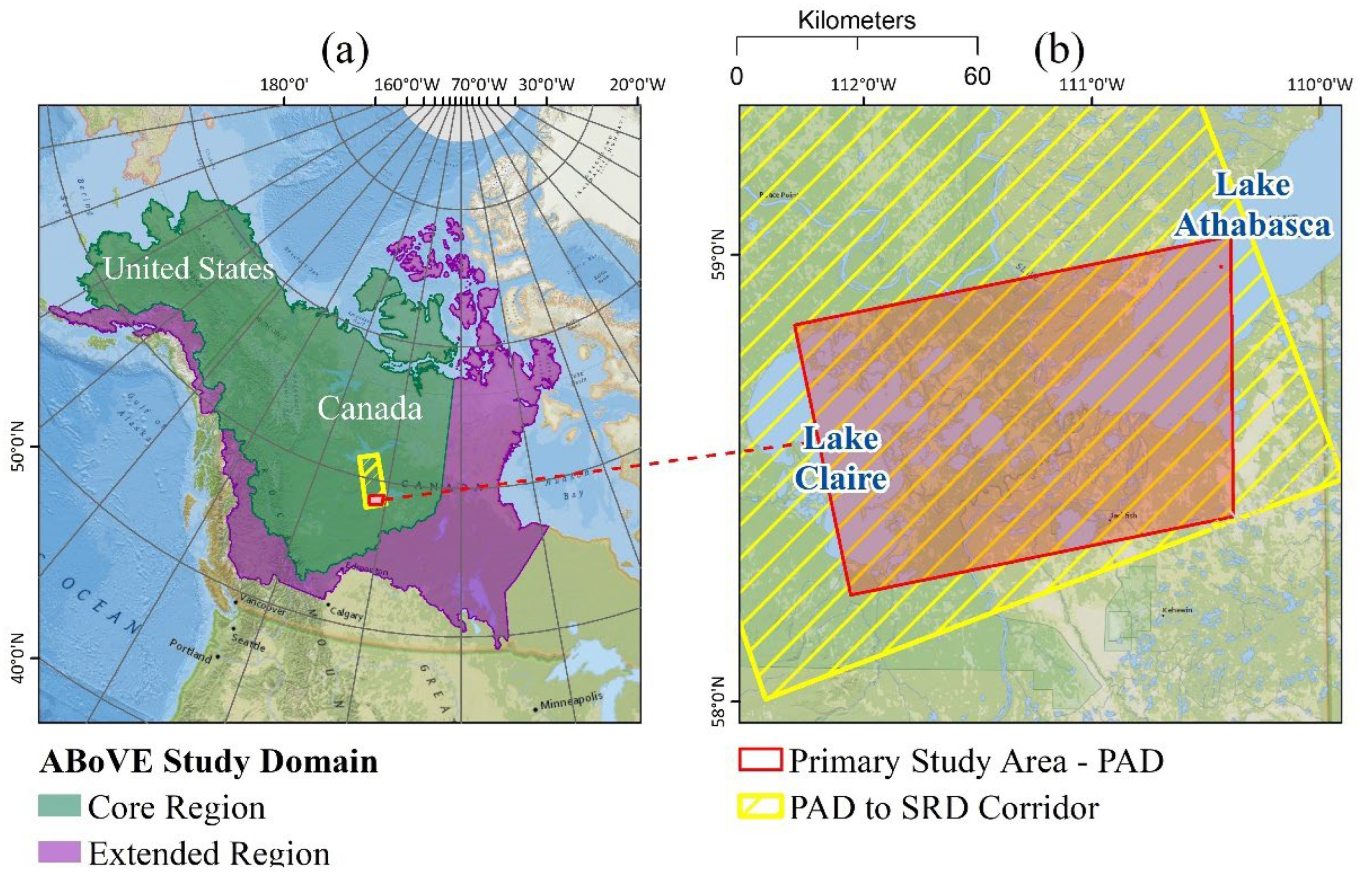
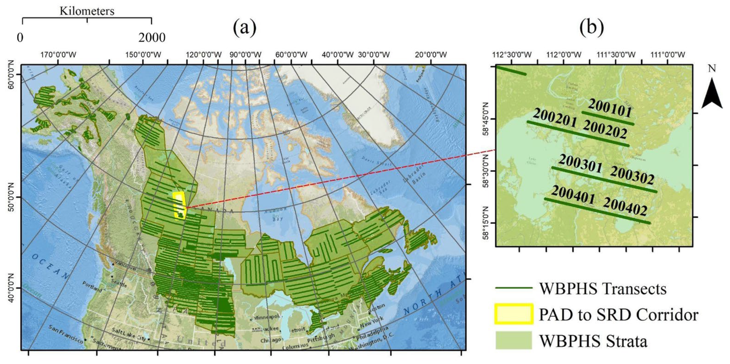
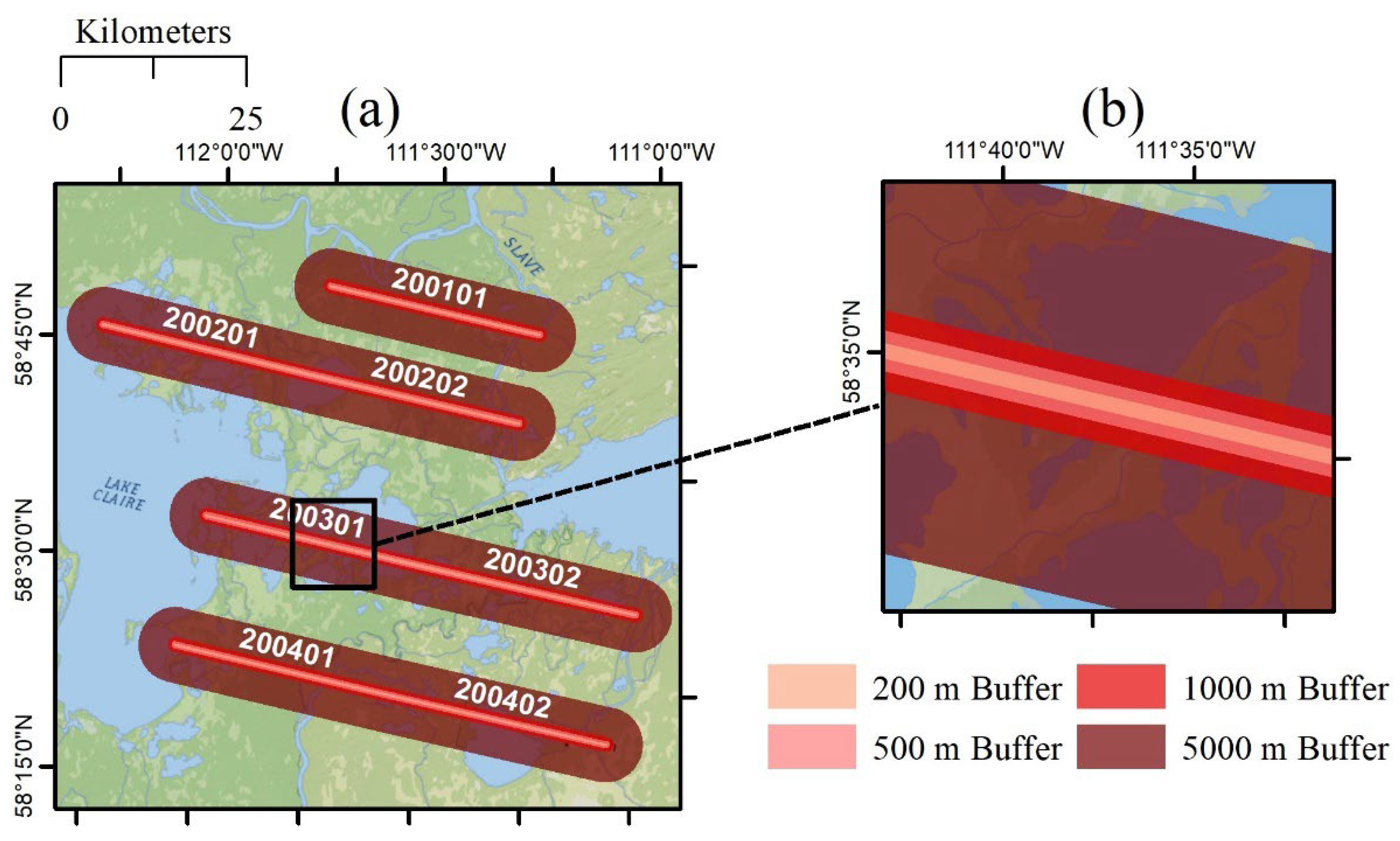
2.1. Study Area

In 2013, NASA commenced the Arctic Boreal Vulnerability Experiment (AboVE) research and field campaign to help address questions related to environmental change in North America’s ABZ [46]. The AboVE campaign provides motivation for studies seeking to leverage remote sensing technologies to better understand the ABZ, particularly under changing climatic conditions. The primary area of interest for our research was the Peace-Athabasca Delta (PAD), Alberta, Canada, located within the core region of the NASA AboVE domain (Figure 1). The PAD has an abundance of hydrologically dynamic lakes and wetlands [34] and is recognized as a Ramsar wetland of international importance. This area also has high duck use and long temporal records of duck survey data, remote sensing information (e.g., both satellite and aerial, including several AboVE airborne campaigns with multiple flight lines; [46]), and current partnerships with indigenous communities. However, we also had available wetland habitat maps over an adjacent region, stretching from the north–south corridor of the PAD to the Slave River Delta (SRD; herein referred to as the PAD to SRD corridor). Our intent was to capitalize on these adjacent data sets to inform some of the preliminary analysis in this study, particularly around the spatial relationships of wetlands at different scales. The duck species abundance models (SAMs) were developed solely over the PAD, as that is where we focused on evaluating the value of our innovative inundation mapping techniques for improving duck models.

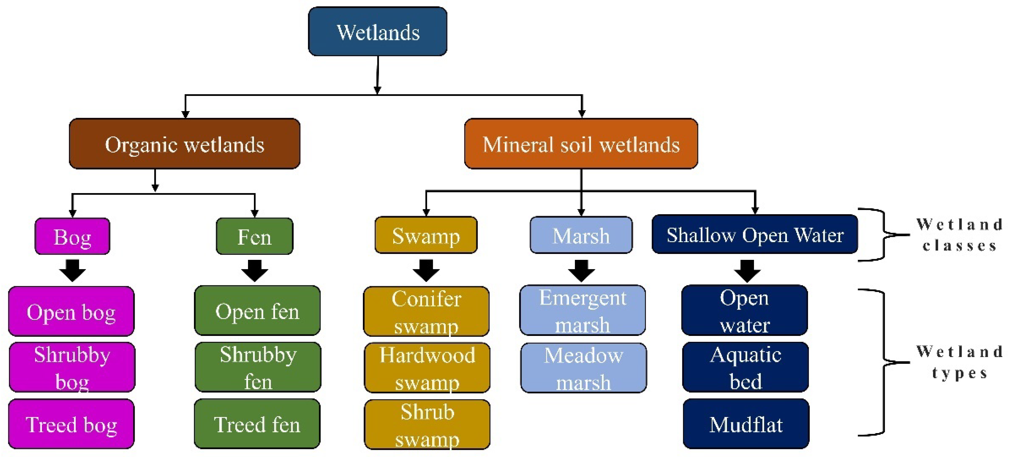
2.2. Wetland Type Mapping

Multi-temporal, multi-source remote sensing data were used to generate a wetland type map representing conditions in the PAD circa 2017. Following Bourgeau-Chavez et al. [47], we used extensive field data to train a Random Forests model [48] on a combination of electro-optical, SAR imagery, and topographic derivatives. For this study, we incorporated electro-optical imagery from Landsat 8, C-band SAR data from Sentinel-1, and L-band SAR data from ALOS-2/PALSAR-2. We also included Height Above Nearest Drainage (HAND) and Topographic Position Indices (TPI) derived from the JAXA ALOS global digital surface model (GDSM) product. The study area was divided into four areas of interest (AOI) for the classification procedure, two covering the PAD, and another two covering a portion of the extended corridor region that connects the Slave River Delta (SRD) to the north that required gap filling. These regions were defined by the frame extents of the available satellite image data. Two ALOS-2/PALSAR-2 images were used for each AOI and collected in dual polarization which transmits horizontally (H) polarized microwave signals and receives both horizontally and vertically (V) polarized backscatter energy (e.g., HH and HV). These images were acquired in Stripmap mode. When possible, we used one image from the beginning of the growing season and another from the end of the growing season, though this was not possible for each AOI due to limited data availability. Two Landsat 8 images representing the early and late growing season were also used in each data stack. Sentinel-1 data are collected more frequently over the ABoVE domain, so mean and standard deviation composites for images collected in the dual-polarization (VV + VH) Interferometric Wide (IW) mode during the growing season were created and incorporated into the data stacks. A table of image types and dates can be found in Appendix A.
Wetland type definitions used for the classification procedure were based on DUC’s Enhanced Wetland Classification (EWC; [40]) system. Minor modifications were made to the EWC classification to better align with the capabilities of the sensors used, for example we did not distinguish between rich and poor fens because they were not separable with the available imagery. We identified 14 wetland types defined by their ecological characteristics (Figure 2). Training and validation polygons representing the 14 wetland types and 4 upland categories (conifer forest, deciduous forest, shrub, and barren land) were generated using field data collected by DUC. A total of 473 polygons were used for the wetland type map, which were randomly divided between training (80%) and validation (20% [49]).

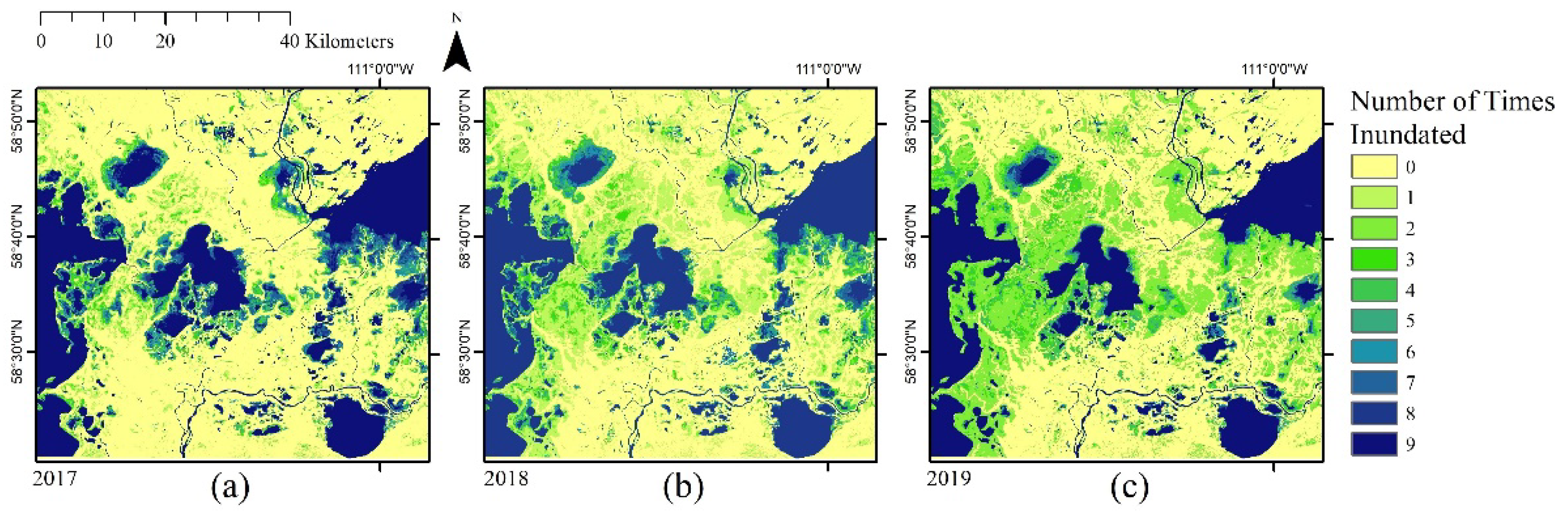
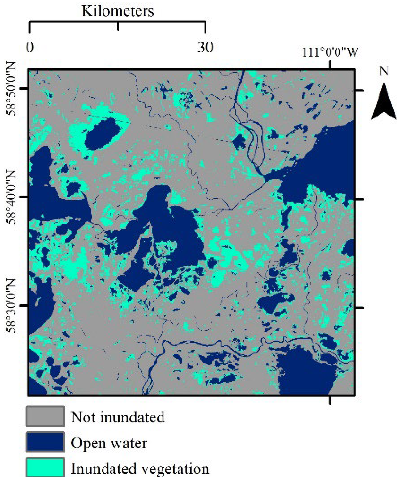
2.3. Wetland Inundation Mapping

Inundation maps were generated over the PAD for each available image collected by Sentinel-1 from late May to the end of August for 2017 to 2019 to create a time-varying product for each year, corresponding to available duck survey data collections. Our method was based on earlier studies using Otsu thresholding techniques applied to RADARSAT-2 (operated by the Canadian Space Agency) C-band SAR data to distinguish open water and flooded vegetation in coastal wetlands in the Laurentian Great Lakes region [50,51]. However, because dense time series data from RADARSAT-2 data was not available for the study region, we instead utilised Sentinel-1 data in the cloud-computing platform Google Earth Engine (GEE). Sentinel-1 data available over Boreal Canada is primarily collected in IW mode, a dual-polarimetric mode consisting of VV and VH bands. Sentinel-1 data in GEE is not radiometrically terrain corrected; however, because the PAD is relatively flat, we proceeded without application of additional corrections to the available data. Before ingestion to the surface water and flooded vegetation detection algorithm, Sentinel-1 images were converted from decibel to linear scale, and speckle filtered using a refined Lee filter with a 7 by 7 window size. The refined Lee filter was used because it preserves edges better than boxcar or median filters. Each image (co-polarized VV and VH cross-polarized components) was then segmented using the Simple Non-Iterative Clustering algorithm [52]. Mean values of VV, VH and their ratio (VV/VH) were calculated for each image segment.
The cross-polarized component (VH) was used to extract surface water because radar scattered off small surface waves of inland lakes is not typically depolarized, resulting in a very low cross-polarized backscatter [33]. To distinguish open water from other cover types, automated Otsu thresholding was applied to a histogram created from a random sample of mean VH backscatter for 10,000 image segments. Image segments with mean values less than the selected threshold were classified as open water.
The ratio of the co-polarized and cross-polarized (VV/VH) backscatter was used to identify flooded vegetation. This metric was used because it tends to be a strong indicator of double-bounce scattering, which is associated with flooded vegetation as incident radiation is reflected off water and then the vertical stem of wetland vegetation (or vice versa) before returning to the sensor. For image segments not categorized as open water, a histogram was generated from a random sample of the mean VV/VH ratio for 10,000 image segments. An Otsu threshold was then selected, with segments greater than the threshold classified as flooded vegetation, and all other segments classified as non-inundated (Figure 3). This type of three-class product was created for all available Sentinel-1 images from the period of study, 2017 to 2019, providing information on sub-seasonal inundation change, the time-variant information used for modelling.

2.4. Duck Abundance Modelling

2.4.1. Duck Survey Data from the WBPHS

Waterfowl Breeding Population and Habitat Survey (WBPHS; [22]) data collected over the PAD for the years 2017–2019 were used to develop duck SAMs. This survey, which has been conducted annually since 1955, represents a large, long-term, and consistent data set collected collaboratively between the U.S. Fish and Wildlife Service (USFWS) and Canadian Wildlife Service (CWS), and has been used extensively for waterfowl modelling (e.g., [21,35,38,39,53]). Aerial transects are flown by the USFWS in fixed-wing aircraft with observers recording the number of waterfowl and ponds. WBPHS survey segments and their spatial extent relative to our general (i.e., the PAD to SRD corridor) and primary area of interest (i.e., the PAD) can be seen in Figure 4. The WBPHS segments typically run east–west and are spaced north–south in varying distances from the southern United States PPR up into Alaska. We partitioned the WBPHS data into two foraging guilds of ducks, diving and dabbling, as these feeding preferences could potentially drive ducks to utilize different depths of water and/or respond differently to inundation conditions. We then used the total count of pairs per segment for diving and dabbling ducks (not adjusted for visibility) as our response variables in SAMs. The total pairs were not adjusted for visibility. The cumulative duck breeding pair count data for each segment over the PAD can be found in Table 1.

2.4.2. Calculation of Spatial Statistics

Habitat characteristics were calculated for the seven WBPHS segments based on the underlying land cover and inundation raster layers over the PAD. These values were then used as covariates for predicting duck pair abundance. The WBPHS segments are represented as polyline features (i.e., rather than as polygons), and so we applied a range of spatial buffers around each segment (200 m, 500 m, 1000 m, and 5000 m) to calculate habitat characteristics at multiple spatial scales (Figure 5). This allowed us to assess the scale dependence of our SAMs.

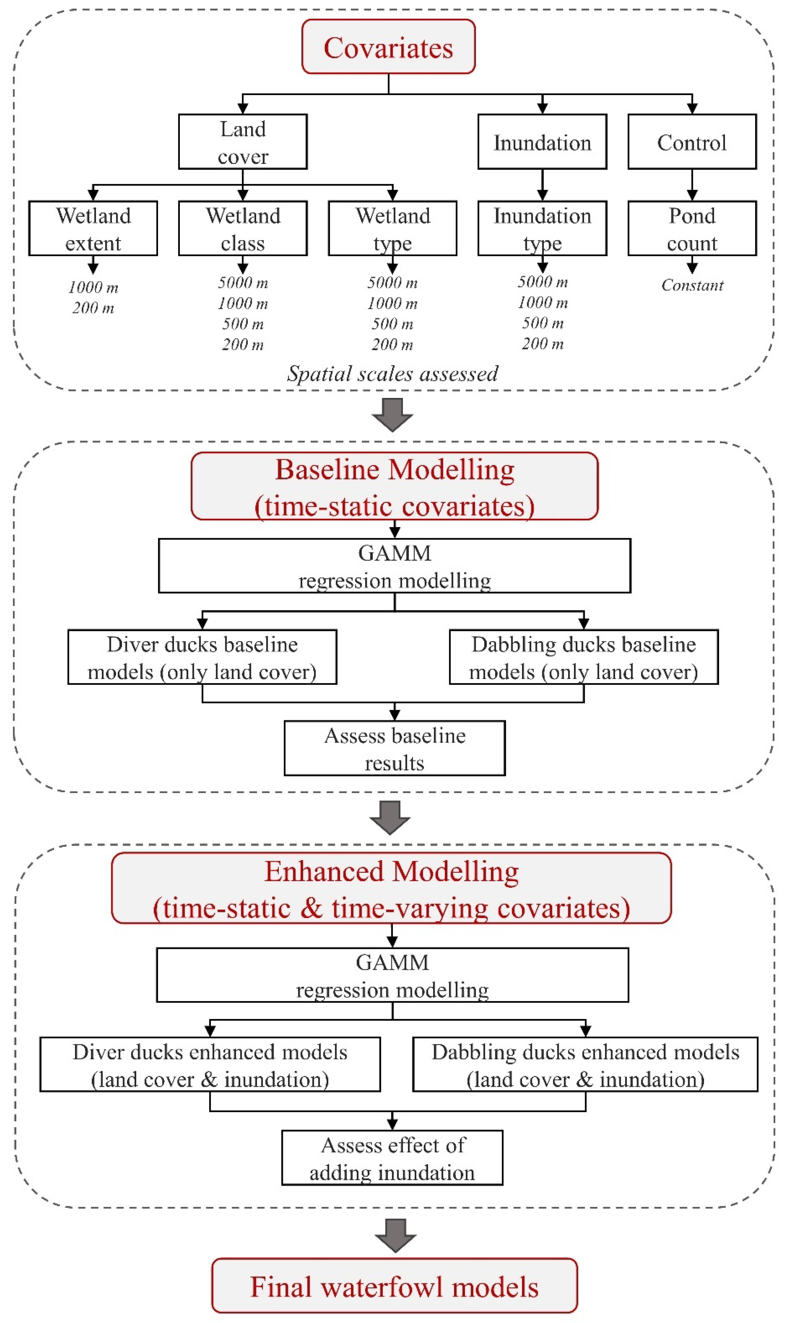
2.4.3. Covariates Used for SAMs

Our duck modelling approach incorporated multiple spatial scales [54], in part to account for the scale-dependent habitat selection processes (e.g., [44]). Key predictors (i.e., covariates) used for duck SAMs were wetland type (time invariant) and inundation (time variant) data. To simplify analyses, some wetland types were collapsed into their higher order wetland classes. Meanwhile, inundation data collected closest but prior to the date to each waterfowl survey were selected for analyses. We also incorporated a more broadly applicable, but coarser and time-invariant wetland habitat layer into SAM analyses, DUC’s Hybrid Wetland Layer (HWL; [55]), which has been used in previous avian modelling studies (e.g., [35]). The HWL is a multi-source mosaicked product that identifies general locations of water and wetlands across Canada, minus the Arctic. As such, this data layer is not robust in determining wetland classes. The HWL was summarized at the 200 m and 1000 m spatial scales, whereas the wetland type, wetland class, and inundation layers were summarized at the 200–5000 m spatial scales. Summaries for each covariate were calculated as the percent (%) area intersecting each WBPHS segment buffer size (Table 2).
We also wanted to control for the variation in ABZ duck population size potentially driven by factors occurring outside the region. Specifically, in dry years in the PPR, ducks are believed to overfly the PPR and settle in the boreal forest [15,16], inflating boreal population sizes independent of boreal habitat conditions. To do this, our SAMs included annual pond count data (i.e., basins which were observed to have water) collected from the US and Canadian prairies during WBPHS surveys (Table 2).

2.4.4. Development of Duck SAMs

Prior to developing SAMs, we performed pairwise correlation (Pearson correlation coefficient; r) analyses on the percent wetland type and class covariates across all spatial scales. This allowed us to explore differences in wetland composition across buffer scales. We used both the PAD and SRD corridor for these analyses (n = 43 WBPHS survey segments), to allow for a more robust assessment of differences in habitat composition across buffer scales than using the PAD alone, and therefore informed our expectations of the role of spatial scale in predicting duck distribution via SAMs.
SAMs were run in a stepwise, additive fashion, separately for each foraging guild because our goal was to test whether the predictive ability provided by the novel inundation data was additive to that from more traditional wetland habitat (i.e., land cover) data. We first modelled duck abundance in the PAD as a function of the time-static covariates-wetland type, class, and extent while controlling for effects of random segment variation and (natural log-transformed) prairie pond counts at each spatial scale. These SAMs are referred to as baseline models. Due to the limited number of survey segments in the PAD (n = 7), only a single time-static covariate was included in each candidate baseline SAM. The best baseline SAMs for each guild were then considered starting models for enhanced SAMs, to which spatio-temporal inundation covariates open water, inundated vegetation, and non-inundated were added at all spatial scales. This approach allowed baseline and enhanced models to compete, hence was an assessment of the additive benefit of inundation covariates on model performance.
SAMs were developed using General Additive Mixed Models (GAMM) and were fit using the ‘mgcv’ library [56] within the R programming language for statistical computing. GAMMs, which allow for the incorporation of random effects, are an extension of generalized additive models and are widely used for modelling correlated and clustered responses; several studies examining waterfowl populations have used this approach [57,58]. Moreover, using GAMM’s allowed covariate effects to be non-linear, with relationship complexities quantified through effective degrees of freedom (EDF; larger values indicate increasingly non-linear model effects). All GAMMs were fit using a natural log link function, negative binomial distribution, and included a smoothed random intercept effect at the segment level. Models were ranked based on Akaike Information Criterion (AIC; [59]), which is a method for identifying best-approximating models (i.e., within 4 Δ AIC units of the top model) among a set of candidates. Our study’s overall approach to modelling duck pair distribution over the PAD is presented in Figure 6.
We then used the best dabbler and diver models from baseline and enhanced SAM analyses to separately predict and map pair abundance across the PAD region. Model-based predicted pairs were generated for reference grids spanning the combined ranges of landcover and inundation covariates in increments of ~0.2–0.3%. Prairie pond counts was set at the mean value across 2017–2019 and the random effect set to 0, resulting in lookup tables containing >40,000 reference pair estimates per guild. The lookup table values were used to plot estimated pair abundance in ArcGIS Pro 3.2.0 software, by assigning abundance for a given pixel based on the wetland covariate attributes summarized at the optimal spatial scale. This resulted in time varying maps for 2017–2019, representing the extent of our inundation data with large lakes masked out.
Pond count data are from the prairies and control for potential influences on boreal population size that occur outside our study area.

3. Results

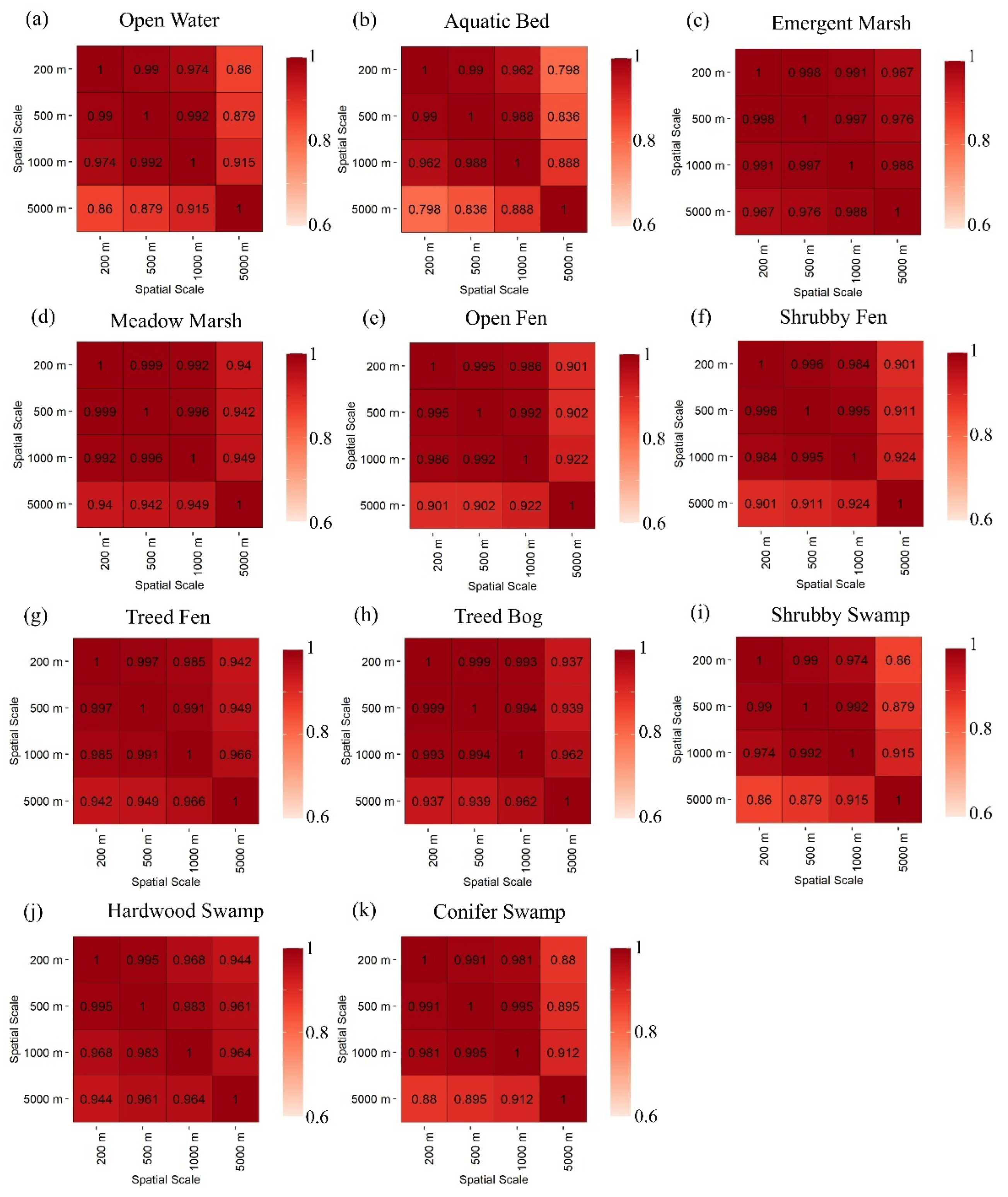
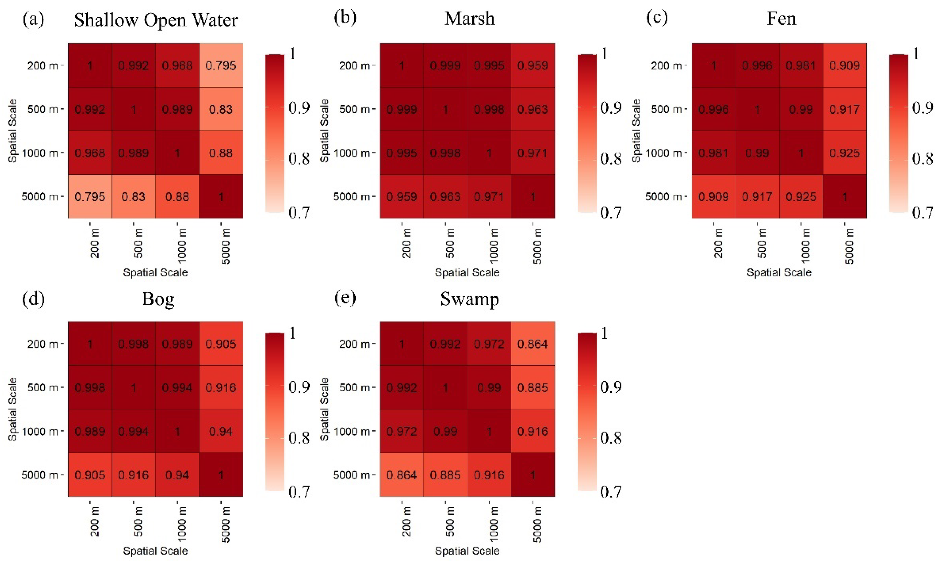
3.1. Pairwise Correlations of Wetland Classes and Types

There was high correlation in percent areas among spatial scales for the five wetland classes (Figure 7, r = 0.79–0.99) and 11 wetland type (Figure 8, r = 0.64–0.98) variables (i.e., the time static wetland variables mapped from this study).

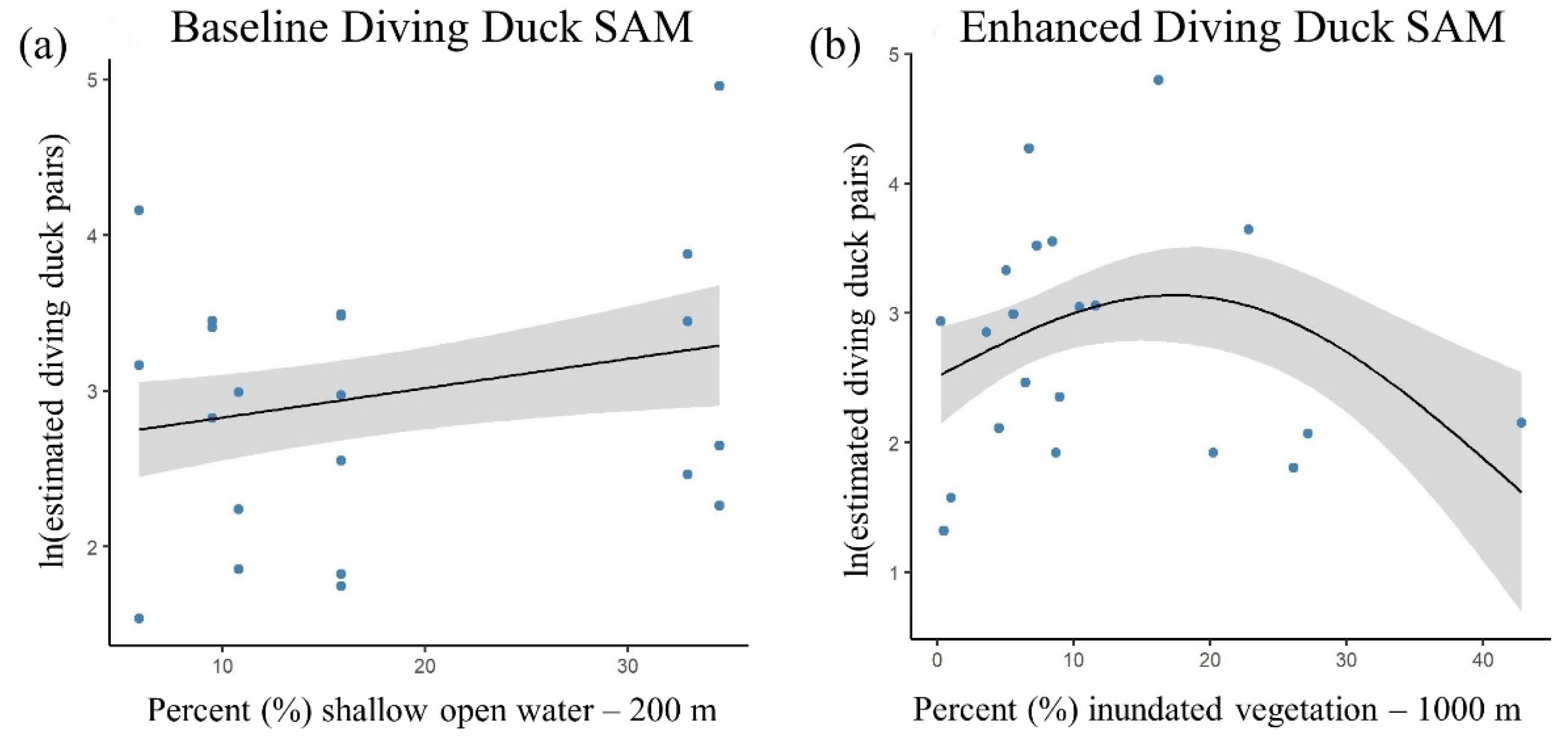
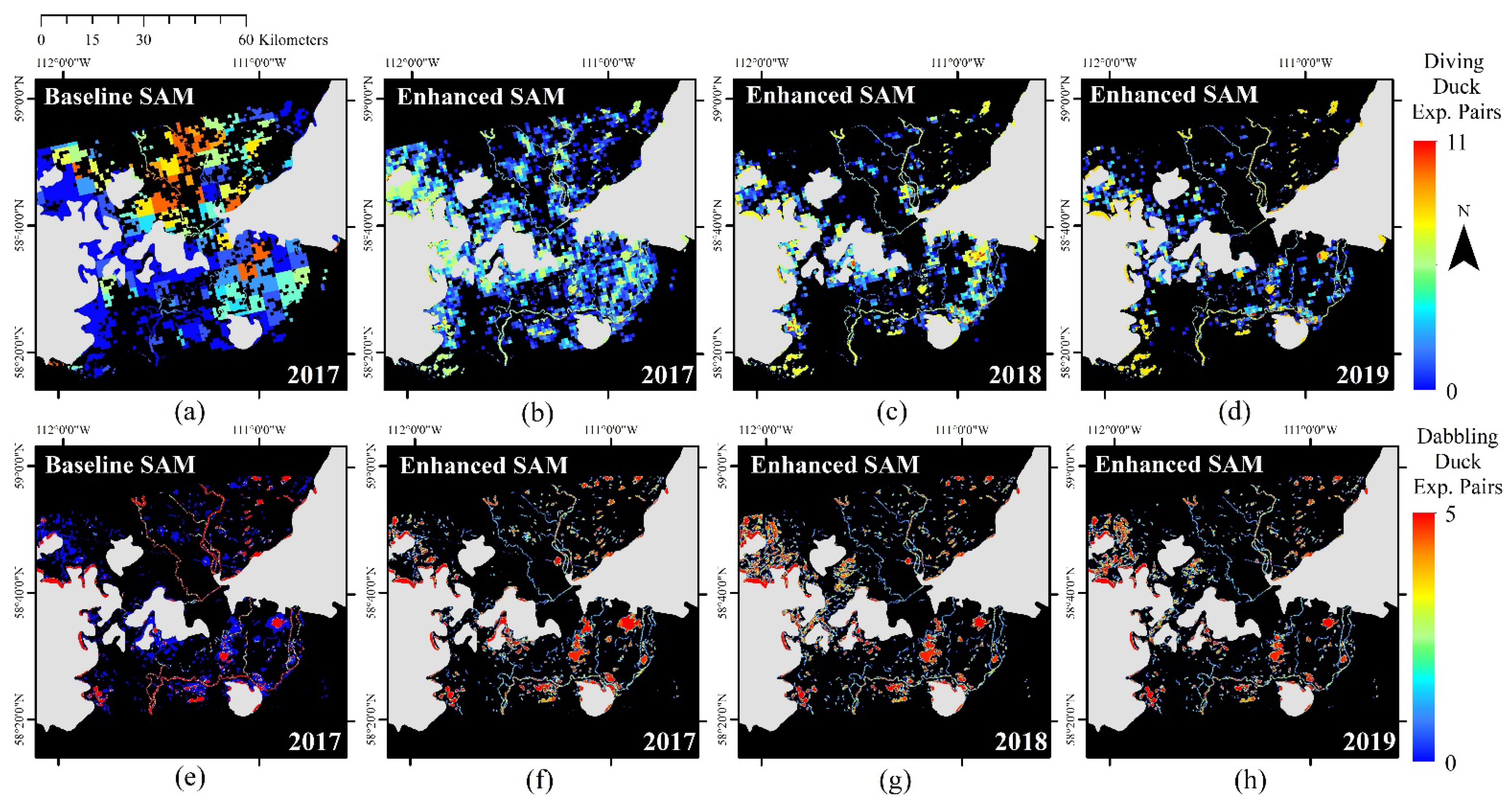
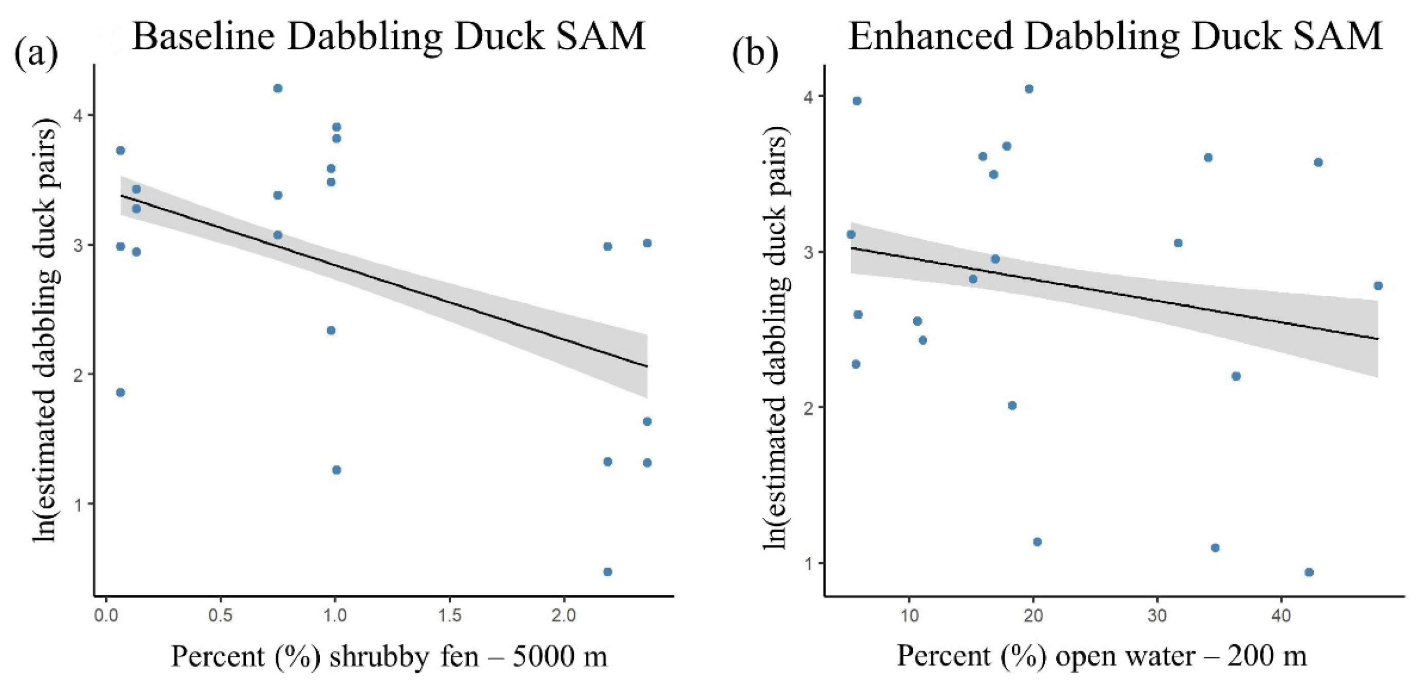
3.2. Baseline Duck SAMs

For diving ducks, the top baseline model was wetland extent open water at 200 m (Table 3). However, because (1) the primary interest of this study was to assess the more detailed wetland type information, (2) very high correlations were observed at all scales within all wetland covariates (Figure 7 and Figure 8), and (3) inclusion of each of these candidate covariates improved on the null model (ΔAIC > 4 from the null model), we advanced both wetland type open water (200 m) and wetland class shallow open water (200 m) to enhanced SAM analyses. Effective degrees of freedom were 1.00 and 1.25, respectively, and we therefore chose to fit them as linear predictors in the enhanced models. Prairie pond counts were not predictive of annual diving duck pair abundance.
Dabbling ducks had several competing baseline models (Table 4), with model fits differing by only ~1.3 AIC units. Two models including either shrubby fen or conifer swamp at 5000 m had significant smoothed covariate effects and so were advanced to enhanced SAM analyses as the best baseline models for dabblers. Effective degrees of freedom for the effects of shrubby fen (5000 m) and conifer swamp (5000 m) were both 1.00 and we therefore fit them as linear predictors in the enhanced models. Dabbling duck pair abundance increased when prairie pond counts were down.

3.3. Enhanced Duck SAMs

For diving ducks, ‘inundated vegetation’ improved baseline models the most, with 5–7 unit decreases in AIC values and a doubling of deviance explained (Table 5). Abundance increased linearly with percent shallow open water (Figure 9) and changed non-linearly with inundated vegetation, increasing until ~20%, then declining thereafter. Note that predictive uncertainty is large at the higher end of observed inundation, given only one observation >30%.
Like diving ducks, time-varying inundation variables improved model performance for dabblers (Table 6). Time-varying open water improved AIC by ~4, although deviance explained the changed minimally. A portion (17%) of deviance explained in the baseline models was due to the random effect of waterfowl survey segment, whereas deviance explained in the enhanced models was due to the biological effects of prairie pond count, land cover, and inundation covariate effects. Dabbling duck pair abundance declined linearly with the percent of both shrubby fen and open water (Figure 10).
Spatial representation of best baseline and enhanced models (Figure 11) further indicates that variability in inundation, including both extent of surface water and inundated vegetation, plays a critical role in determining abundance and distribution of duck pairs. Specifically, variations in model inputs (e.g., time static, or time varying) can lead to very different duck population estimates. For example, in some cases, the enhanced SAMs either identified important regions missed by the baseline SAMs or had substantially different portrayals of where high-density locations were located.

4. Discussion

Our study demonstrated the potential value of using novel remote sensing data, in particular SAR, to advance conservation of biodiversity in remote regions. Not only did models using time-variant SAR data statistically outperform time-static models, but they also allowed for more frequent prediction of changes in species abundance and distribution (e.g., from year-to-year). Thus, we see potential to use SAMs and SAR wetland data to undertake regular, predictive population estimation in response to observed habitat changes. In addition, the improved modelling capabilities allowed by SAR wetland data could facilitate better forecasting of how abundance and distribution of wetland-dependent species respond to future habitat change scenarios in northern regions. This could even have implications for public health, in terms of epidemiology. Since waterfowl are natural carriers of pathogens, understanding their habitat preferences could provide valuable insights into their migration patterns and thus virus transmission [60].
The biodiversity conservation benefits of such ability to estimate or forecast changes in abundance and distribution based on habitat characteristics is significant [61,62,63]. Climate change is expected to have habitat altering consequences for wetland-dependent species [9] but is not the only source of potential change to the ABZ habitat. Resource extraction may alter wetlands in the region [64,65], which could require measures to avoid negative consequences for biodiversity. Any such conservation effort requires an understanding of where important areas are, why they are important, and, ideally, how robust the value of those areas may be to systematic habitat changes such as loss, degradation, or shifts in location or types. This understanding helps planners assess where best to apply conservation measures, what actions are likely to be most effective and, ultimately, whether they are successful. Our results with SAR data suggest that the relative importance of different regions may vary with habitat conditions. If true, SAMs based on time-invariant habitat data may not accurately identify locations of important areas because inputs are only a snapshot of dynamic systems. As well, the ability that SAMs and SAR data may provide for monitoring animal population response to changing habitat conditions can be a cornerstone of model-based metrics of conservation success, permitting rapid learning and adaptation. These metrics are particularly beneficial when status and trend surveys to directly measure population response are too costly, infrequent, or sparse relative to the pace and needs of decision making, which is likely true for much of the ABZ.
The comprehensive characterization of wetlands in the ABZ, both in terms of classification (e.g., type) and condition (e.g., inundation), has implications beyond biodiversity conservation. Climate modelling suggests that arctic amplification/climate change is altering the biogeochemical cycling of ABZ wetlands, causing instabilities that are shifting some from a greenhouse gas sink to source, and further threatening their role in the global hydrological cycle and climate regulation at large [66,67]. Recent studies suggest long-term warming is enhancing these processes, in which positive greenhouse-gas–climate feedback is associated with wetland hydrological regime shifts [68]. ABZ wetlands are evidently complex ecosystems that are sensitive to environmental shifts [5,69], and to fully understand their hydrological properties when subject to increasing global temperatures, and implications for biodiversity more broadly, enhanced remote sensing methods such as ours can be used.
Monitoring of wetland conditions is a challenging task in more remote regions of the world, such as the ABZ [70]. The GEE cloud-based image processing pipeline presented in this study represents an efficient and potentially scalable solution to deriving such critical biodiversity-related information over extensive areas (e.g., the NASA ABoVE domain). Traditional remote sensing techniques use desktop-based processing and specific software to map wetland conditions [71]. However, this study adopted a cloud-based framework based on GEE’s on-demand resource allocation and processing capabilities [72]. Using GEE and weather-independent SAR imagery permits frequent (e.g., 6-to-12-day revisit time based on Sentinel-1) and consistent monitoring of wetlands, data which can be used to model wetland conditions under different and/or changing climatic conditions, both among and within year. For example, our analyses used inundation at a single time stamp each year corresponding to waterfowl survey dates. However, our mapping approach also permits assessment of annual variation in inundation frequency (Figure 12). These hydroperiod maps were created by combining ‘open water’ and ‘inundated vegetation’ pixels for each Sentinel-1 satellite revisit into one general ‘inundated’ class, then calculating inundation frequency based on how often a pixel was classified as inundated across satellite revisits within a year. Clearly, wetland hydroperiod can be very different from year to year, which is closely linked to precipitation and evapotranspiration [73] and may have implications for wetland productivity and biodiversity [74]. This makes maps like these important for assessing habitat as climate change continues to impact the extent and dynamics of wetlands in the ABZ of North America [75].
For these reasons, SAR imagery represents an advantageous approach to wetland monitoring compared to conventional optical sensors which are impeded by cloud cover [76]. SAR sensors also have canopy penetrating capabilities, providing valuable information on beneath canopy flooding which would otherwise be missed with optical data [77] and can be critical to informing biodiversity conservation. As such, our future intention is to test the feasibility of this inundation methodology over different regions of the ABZ for informing duck SAMs and other indices useful to biodiversity conservation. Further demonstration would permit development of duck SAMs at the scale of the ABoVE domain, improving targeted conservation initiatives [53,78,79,80].

5. Conclusions

The results of this study demonstrated that novel, time-varying inundation information produced using SAR satellite imagery and cloud computing enhanced our ability to predict duck pair abundance in an ABZ study site. Specifically, inundated vegetation and open surface water successfully captured the inter- and intra-annual dynamics of wetlands, resulting in better SAMs than baseline land cover-only data, which is what previous studies have mostly relied on in the ABZ. This outcome suggests that incorporating inundation into duck pair abundance and/or distribution models at larger scales could lead to better and more frequent predictability, an asset for conservation planning in northern environments, particularly in the context of climate-related and other habitat changes. This enhanced spatio-temporal information may also be important for supporting indigenous subsistence harvest of waterfowl and assisting in indigenous-led conservation planning that is both effective and socially just.

Author Contributions

Study conceptualization and oversight, N.F., S.S., K.S. and V.B.H.; SAR methodology development, processing, and inundation mapping, M.J.B.; duck model development and statistical analysis, L.A. and H.V.S.; duck survey data collection, H.V.S.; GIS analysis, mapping, and applications, M.A.M.; original manuscript preparation, M.A.M.; manuscript review and editing, M.J.B., N.F., H.V.S., L.A., V.B.H. and S.S.; funding acquisition, N.F. and K.S. All authors have read and agreed to the published version of the manuscript.

Funding

This work was supported by NASA’s ABoVE program (grant 80NSSC19M0108).

Data Availability Statement

The data presented in this study are available on request from the corresponding author.

Acknowledgments

We are thankful to the USFWS for making the BPOP data publicly available. We also want to acknowledge that this research was conducted over Treaty 8 territory, and we honor and acknowledge all of the First Nations, Métis and Inuit peoples who have lived, travelled and gathered on these lands for thousands of years.

Conflicts of Interest

Michael Allan Merchant, Howie Singer, Llwellyn Armstrong, Vanessa B. Harriman and Stuart Slattery are employed by Ducks Unlimited Canada. Michael Allan Merchant is employed by First Resource Management Group, SkyForest. Kevin Smith is employed by Habitat Acquisition Trust. The remaining authors declare no conflicts of interest.

Appendix A

Table A1. Remote sensing image sources and their acquisition dates used for wetland type classification of the Peace-Athabasca Delta (PAD) and for parts of the extended corridor region covering the Slave River Delta (SRD).
AOIPALSAR-2 Date 1PALSAR-2 Date 2Landsat 8 Date 1Landsat 8 Date 2Sentinel-1 Date Ranges
PAD East2 July 20183 July 201728 May 201926 August 20172 June 2017–20 August 2018
PAD West17 July 201727 August 201828 May 201926 August 20172 June 2017–20 August 2018
SRD East2 July 201821 July 201814 June 201717 August 201712 June 2017–20 August 2018
SRD West28 June 201821 July 201830 May 201831 August 201712 June 2017–18 August 2019

References

  1. Olefeldt, D.; Hovemyr, M.; Kuhn, M.A.; Bastviken, D.; Bohn, T.J.; Connolly, J.; Crill, P.; Euskirchen, E.S.; Finkelstein, S.A.; Genet, H.; et al. The Boreal–Arctic Wetland and Lake Dataset (BAWLD). Earth Syst. Sci. Data 2021, 13, 5127–5149. [Google Scholar] [CrossRef]
  2. Wrona, F.; Reist, J.; Lehtonen, H.; Kahilainen, K.; Forsstrom, L.; Wrona, F.; Reist, J.; Amundsen, P.; Chambers, P.; Christoffersen, K.; et al. Freshwater Ecosystems. In Arctic Biodiversity Assessment: Status and Trends in Arctic Biodiversity; Narayana Press: Odder, Denmark, 2013; pp. 443–485. [Google Scholar]
  3. Hofgaard, A.; Harper, K.; Golubeva, E. The Role of the Circumarctic Forest–Tundra Ecotone for Arctic Biodiversity. Biodiversity 2012, 13, 174–181. [Google Scholar] [CrossRef]
  4. Berteaux, D.; Gauthier, G.; Domine, F.; Ims, R.A.; Lamoureux, S.F.; Lévesque, E.; Yoccoz, N. Effects of Changing Permafrost and Snow Conditions on Tundra Wildlife: Critical Places and Times. Arct. Sci. 2017, 3, 65–90. [Google Scholar] [CrossRef]
  5. Kreplin, H.N.; Santos Ferreira, C.S.; Destouni, G.; Keesstra, S.D.; Salvati, L.; Kalantari, Z. Arctic Wetland System Dynamics under Climate Warming. Wiley Interdiscip. Rev. Water 2021, 8, e1526. [Google Scholar] [CrossRef]
  6. Previdi, M.; Smith, K.; Polvani, L. Arctic Amplification of Climate Change: A Review of Underlying Mechanisms. Environ. Res. Lett. 2021, 16, 093003. [Google Scholar] [CrossRef]
  7. Rawlins, M.A.; Steele, M.; Holland, M.M.; Adam, J.C.; Cherry, J.E.; Francis, J.A.; Groisman, P.Y.; Hinzman, L.D.; Huntington, T.G.; Kane, D.L.; et al. Analysis of the Arctic System for Freshwater Cycle Intensification: Observations and Expectations. J. Clim. 2010, 23, 5715–5737. [Google Scholar] [CrossRef]
  8. Cohen, J.; Screen, J.A.; Furtado, J.C.; Barlow, M.; Whittleston, D.; Coumou, D.; Francis, J.; Dethloff, K.; Entekhabi, D.; Overland, J.; et al. Recent Arctic Amplification and Extreme Mid-Latitude Weather. Nat. Geosci. 2014, 7, 627–637. [Google Scholar] [CrossRef]
  9. Wrona, F.J.; Johansson, M.; Culp, J.M.; Jenkins, A.; Mård, J.; Myers-Smith, I.H.; Prowse, T.D.; Vincent, W.F.; Wookey, P.A. Transitions in Arctic Ecosystems: Ecological Implications of a Changing Hydrological Regime. J. Geophys. Res. Biogeosci. 2016, 121, 650–674. [Google Scholar] [CrossRef]
  10. Kåresdotter, E.; Destouni, G.; Ghajarnia, N.; Hugelius, G.; Kalantari, Z. Mapping the Vulnerability of Arctic Wetlands to Global Warming. Earths Future 2021, 9, e2020EF001858. [Google Scholar] [CrossRef]
  11. Chen, J.; Brissette, F.P.; Poulin, A.; Leconte, R. Overall Uncertainty Study of the Hydrological Impacts of Climate Change for a Canadian Watershed. Water Resour. Res. 2011, 47, W12509. [Google Scholar] [CrossRef]
  12. Taylor, J.J.; Lawler, J.P.; Aronsson, M.; Barry, T.; Bjorkman, A.D.; Christensen, T.; Coulson, S.J.; Cuyler, C.; Ehrich, D.; Falk, K.; et al. Arctic Terrestrial Biodiversity Status and Trends: A Synopsis of Science Supporting the CBMP State of Arctic Terrestrial Biodiversity Report. Ambio 2020, 49, 833–847. [Google Scholar] [CrossRef] [PubMed]
  13. Slattery, S.; Morissette, J.; Mack, G.; Butterworth, E. Waterfowl Conservation Planning. In Boreal Birds of North America: A Hemispheric View of Their Conservation Links and Significance; University of California Press: Berkeley, CA, USA, 2011; pp. 23–41. [Google Scholar]
  14. Holopainen, S.; Arzel, C.; Dessborn, L.; Elmberg, J.; Gunnarsson, G.; Nummi, P.; Pöysä, H.; Sjöberg, K. Habitat Use in Ducks Breeding in Boreal Freshwater Wetlands: A Review. Eur. J. Wildl. Res. 2015, 61, 339–363. [Google Scholar] [CrossRef]
  15. Kusack, J.; Tozer, D.; Schummer, M.; Hobson, K. Origins of Harvested American Black Ducks: Stable Isotopes Support the Flyover Hypothesis. J. Wildl. Manag. 2023, 87, e22324. [Google Scholar] [CrossRef]
  16. Runge, M.; Boomer, G. Population Dynamics and Harvest Management of the Continental Northern Pintail Population; Division of Migratory Bird Management, United States Fish and Wildlife Service: Washington, DC, USA, 2005.
  17. Prosser, D.J.; Ding, C.; Erwin, R.M.; Mundkur, T.; Sullivan, J.D.; Ellis, E.C. Species Distribution Modeling in Regions of High Need and Limited Data: Waterfowl of China. Avian Res. 2018, 9, 7. [Google Scholar] [CrossRef]
  18. Tsuji, L.; Wilton, M.; Spiegelaar, N.; Oelbermann, M.; Barbeau, C.; Solomon, A.; Tsuji, C.; Liberda, E.; Meldrum, R.; Karagatzides, J. Enhancing Food Security in Subarctic Canada in the Context of Climate Change: The Harmonization of Indigenous Harvesting Pursuits and Agroforestry Activities to Form a Sustainable Import-Substitution Strategy. In Sustainable Solutions for Food Security: Combating Climate Change by Adaptation; Springer: Cham, Switzerland, 2019; pp. 409–435. [Google Scholar]
  19. Steen, V.A.; Skagen, S.K.; Melcher, C.P. Implications of Climate Change for Wetland-Dependent Birds in the Prairie Pothole Region. Wetlands 2016, 36, 445–459. [Google Scholar] [CrossRef]
  20. Ballard, D.C.; Jones, O.E.; Janke, A.K. Factors Affecting Wetland Use by Spring Migrating Ducks in the Southern Prairie Pothole Region. J. Wildl. Manag. 2021, 85, 1490–1506. [Google Scholar] [CrossRef]
  21. Doherty, K.E.; Evans, J.S.; Walker, J.; Devries, J.H.; Howerter, D.W. Building the Foundation for International Conservation Planning for Breeding Ducks across the U.S. and Canadian Border. PLoS ONE 2015, 10, e0116735. [Google Scholar] [CrossRef]
  22. Smith, W. A Critical Review of the Aerial and Ground Surveys of Breeding Waterfowl in North America; National Biological Service: Laurel, MD, USA, 1995.
  23. Niemuth, N.D.; Solberg, J.W. Response of Waterbirds to Number of Wetlands in the Prairie Pothole Region of North Dakota, U.S.A. Waterbirds 2003, 26, 233–238. [Google Scholar] [CrossRef]
  24. Wong, L.; Cornelis Van Kooten, G.; Clarke, J.A. Search the Impact of Agriculture on Waterfowl Abundance: Evidence from Panel Data. J. Agric. Resour. Econ. 2012, 37, 321–334. [Google Scholar]
  25. Walker, J.; Rotella, J.J.; Stephens, S.E.; Lindberg, M.S.; Ringelman, J.K.; Hunter, C.; Smith, A.J. Time-Lagged Variation in Pond Density and Primary Productivity Affects Duck Nest Survival in the Prairie Pothole Region. Ecol. Appl. 2013, 23, 1061–1074. [Google Scholar] [CrossRef]
  26. Niemuth, N.D.; Fleming, K.K.; Reynolds, R.E. Waterfowl Conservation in the US Prairie Pothole Region: Confronting the Complexities of Climate Change. PLoS ONE 2014, 9, e100034. [Google Scholar] [CrossRef]
  27. McIntyre, N.E.; Liu, G.; Gorzo, J.; Wright, C.K.; Guntenspergen, G.R.; Schwartz, F. Simulating the Effects of Climate Variability on Waterbodies and Wetland-Dependent Birds in the Prairie Pothole Region. Ecosphere 2019, 10, e02711. [Google Scholar] [CrossRef]
  28. Beamish, A.; Raynolds, M.; Epstein, H.; Frost, G.; Macander, M.; Bergstedt, H.; Bartsch, A.; Kruse, S.; Miles, V.; Tanis, C.; et al. Recent Trends and Remaining Challenges for Optical Remote Sensing of Arctic Tundra Vegetation: A Review and Outlook. Remote Sens. Environ. 2020, 246, 111872. [Google Scholar] [CrossRef]
  29. Yang, D.; Kane, D. Arctic Hydrology, Permafrost and Ecosystems; Springer Nature: Berlin/Heidelberg, Germany, 2020. [Google Scholar]
  30. Cooley, S.; Smith, L.; Ryan, J.; Pitcher, L.; Pavelsky, T. Arctic-Boreal Lake Dynamics Revealed Using CubeSat Imagery. Geophys. Res. Lett. 2019, 46, 2111–2120. [Google Scholar] [CrossRef]
  31. Carroll, M.; Wooten, M.; DiMiceli, C.; Sohlberg, R.; Kelly, M. Quantifying Surface Water Dynamics at 30 Meter Spatial Resolution in the North American High Northern Latitudes 1991–2011. Remote Sens. 2016, 8, 622. [Google Scholar] [CrossRef]
  32. Schumann, G.; Giustarini, L.; Tarpanelli, A.; Jarihani, B.; Martinis, S. Flood Modeling and Prediction Using Earth Observation Data. Surv. Geophys. 2023, 44, 1553–1578. [Google Scholar] [CrossRef]
  33. Brisco, B. Mapping and monitoring surface water and wetlands with synthetic aperture radar. In Remote Sensing of Wetlands: Applications and Advances; CRC Press: Boca Raton, FL, USA, 2015; pp. 119–136. [Google Scholar]
  34. Huang, C.; Smith, L.C.; Kyzivat, E.D.; Fayne, J.V.; Ming, Y.; Spence, C. Tracking Transient Boreal Wetland Inundation with Sentinel-1 SAR: Peace-Athabasca Delta, Alberta and Yukon Flats, Alaska. GIsci Remote Sens. 2022, 59, 1767–1792. [Google Scholar] [CrossRef]
  35. Barker, N.; Cumming, S.; Darveau, M. Models to Predict the Distribution and Abundance of Breeding Ducks in Canada. Avian Conserv. Ecol. 2014, 9, 7. [Google Scholar] [CrossRef]
  36. Smith, P.A.; McKinnon, L.; Meltofte, H.; Lanctot, R.B.; Fox, A.D.; Leafloor, J.O.; Soloviev, M.; Franke, A.; Falk, K.; Golovatin, M.; et al. Status and Trends of Tundra Birds across the Circumpolar Arctic. Ambio 2020, 49, 732–748. [Google Scholar] [CrossRef]
  37. Adde, A.; Darveau, M.; Barker, N.; Cumming, S. Predicting Spatiotemporal Abundance of Breeding Waterfowl across Canada: A Bayesian Hierarchical Modelling Approach. Divers. Distrib. 2020, 26, 1248–1263. [Google Scholar] [CrossRef]
  38. Singer, H.V.; Slattery, S.M.; Armstrong, L.; Witherly, S. Assessing Breeding Duck Population Trends Relative to Anthropogenic Disturbances across the Boreal Plains of Canada, 1960–2007. Avian Conserv. Ecol. 2020, 15, 1. [Google Scholar] [CrossRef]
  39. Adde, A.; Casabona i Amat, C.; Mazerolle, M.J.; Darveau, M.; Cumming, S.G.; O’Hara, R.B. Integrated Modeling of Waterfowl Distribution in Western Canada Using Aerial Survey and Citizen Science (EBird) Data. Ecosphere 2021, 12, e03790. [Google Scholar] [CrossRef]
  40. Smith, K.; Smith, C.; Forest, S.; Richard, A. A Field Guide to the Wetlands of the Boreal Plains Ecozone of Canada; Ducks Unlimited Canada, Western Boreal Office: Edmonton, AB, Canada, 2007.
  41. Merchant, M.A.; Warren, R.K.; Edwards, R.; Kenyon, J.K. An Object-Based Assessment of Multi-Wavelength SAR, Optical Imagery and Topographical Datasets for Operational Wetland Mapping in Boreal Yukon, Canada. Can. J. Remote Sens. 2019, 45, 308–332. [Google Scholar] [CrossRef]
  42. Merchant, M.; Haas, C.; Schroder, J.; Warren, R.; Edwards, R. High-Latitude Wetland Mapping Using Multidate and Multisensor Earth Observation Data: A Case Study in the Northwest Territories. J. Appl. Remote Sens. 2020, 14, 034511. [Google Scholar] [CrossRef]
  43. Wright, J.R.; Johnson, J.A.; Bayne, E.; Powell, L.L.; Foss, C.R.; Kennedy, J.C.; Marra, P.P. Migratory Connectivity and Annual Cycle Phenology of Rusty Blackbirds (Euphagus Carolinus) Revealed through Archival Gps Tags. Avian Conserv. Ecol. 2021, 16, 20. [Google Scholar] [CrossRef]
  44. Dyson, M.E.; Slattery, S.M.; Fedy, B.C. Multiscale Nest-Site Selection of Ducks in the Western Boreal Forest of Alberta. Ecol. Evol. 2022, 12, e9139. [Google Scholar] [CrossRef]
  45. Kahara, S.N.; Skalos, D.; Madurapperuma, B.; Hernandez, K. Habitat Quality and Drought Effects on Breeding Mallard and Other Waterfowl Populations in California, USA. J. Wildl. Manag. 2022, 86, e22133. [Google Scholar] [CrossRef]
  46. Miller, C.E.; Griffith, P.C.; Goetz, S.J.; Hoy, E.E.; Pinto, N.; McCubbin, I.B.; Thorpe, A.K.; Hofton, M.; Hodkinson, D.; Hansen, C.; et al. An Overview of above Airborne Campaign Data Acquisitions and Science Opportunities. Environ. Res. Lett. 2019, 14, 080201. [Google Scholar] [CrossRef]
  47. Bourgeau-Chavez, L.; Endres, S.; Powell, R.; Battaglia, M.; Benscoter, B.; Turetsky, M.; Kasischke, E.; Banda, E. Mapping Boreal Peatland Ecosystem Types from Multitemporal Radar and Optical Satellite Imagery. Can. J. For. Res. 2017, 47, 545–559. [Google Scholar] [CrossRef]
  48. Breiman, L. Random Forests. Mach. Learn. 2001, 45, 5–32. [Google Scholar] [CrossRef]
  49. Martins, V.S.; Kaleita, A.L.; Gelder, B.K.; Nagel, G.W.; Maciel, D.A. Deep Neural Network for Complex Open-Water Wetland Mapping Using High-Resolution WorldView-3 and Airborne LiDAR Data. Int. J. Appl. Earth Obs. Geoinf. 2020, 93, 102215. [Google Scholar] [CrossRef]
  50. Behnamian, A.; Banks, S.; White, L.; Brisco, B.; Milard, K.; Pasher, J.; Chen, Z.; Duffe, J.; Bourgeau-Chavez, L.; Battaglia, M. Semi-Automated Surfacewater Detection with Synthetic Aperture Radar Data: A Wetland Case Study. Remote Sens. 2017, 9, 1209. [Google Scholar] [CrossRef]
  51. Battaglia, M.J.; Banks, S.; Behnamian, A.; Bourgeau-Chavez, L.; Brisco, B.; Corcoran, J.; Chen, Z.; Huberty, B.; Klassen, J.; Knight, J.; et al. Multi-Source Eo for Dynamic Wetland Mapping and Monitoring in the Great Lakes Basin. Remote Sens. 2021, 13, 599. [Google Scholar] [CrossRef]
  52. Achanta, R.; Susstrunk, S. Superpixels and Polygons Using Simple Non-Iterative Clustering. In Proceedings of the IEEE Conference on Computer Vision and Pattern Recognition, Honolulu, HI, USA, 21–26 July 2017; pp. 4651–4660. [Google Scholar]
  53. Kemink, K.M.; Adams, V.M.; Pressey, R.L. Integrating Dynamic Processes into Waterfowl Conservation Prioritization Tools. Divers. Distrib. 2021, 27, 585–601. [Google Scholar] [CrossRef]
  54. Tozer, D.C.; Stewart, R.L.M.; Steele, O.; Gloutney, M. Species-Habitat Relationships and Priority Areas for Marsh-Breeding Birds in Ontario. J. Wildl. Manag. 2020, 84, 786–801. [Google Scholar] [CrossRef]
  55. Jones, N. Hybrid Wetland Layer (Version 2.1) User Guide; Ducks Unlimited Canada: Edmonton, AB, Canada, 2010.
  56. Wood, S. Mixed GAM Computation Vehicle with Automatic Smoothness Estimation; Version 1.8-40; RStudio: Vienna, Austria, 2022. [Google Scholar]
  57. Wen, L.; Rogers, K.; Saintilan, N.; Ling, J. The Influences of Climate and Hydrology on Population Dynamics of Waterbirds in the Lower Murrumbidgee River Floodplains in Southeast Australia: Implications for Environmental Water Management. Ecol. Model. 2011, 222, 154–163. [Google Scholar] [CrossRef]
  58. Nykänen, M.; Pöysä, H.; Hakkarainen, S.; Rajala, T.; Matala, J.; Kunnasranta, M. Seasonal and Diel Activity Patterns of the Endangered Taiga Bean Goose (Anser fabalis fabalis) during the Breeding Season, Monitored with Camera Traps. PLoS ONE 2021, 16, e0254254. [Google Scholar] [CrossRef]
  59. Cavanaugh, J.E.; Neath, A.A. The Akaike Information Criterion: Background, Derivation, Properties, Application, Interpretation, and Refinements. Wiley Interdiscip. Rev. Comput. Stat. 2019, 11, e1460. [Google Scholar] [CrossRef]
  60. Roberts, N.J.; Krilov, L.R. The Continued Threat of Influenza A Viruses. Viruses 2022, 14, 883. [Google Scholar] [CrossRef]
  61. Didham, R.K.; Tylianakis, J.M.; Gemmell, N.J.; Rand, T.A.; Ewers, R.M. Interactive Effects of Habitat Modification and Species Invasion on Native Species Decline. Trends Ecol. Evol. 2007, 22, 489–496. [Google Scholar] [CrossRef]
  62. Venier, L.A.; Thompson, I.D.; Fleming, R.; Malcolm, J.; Aubin, I.; Trofymow, J.A.; Langor, D.; Sturrock, R.; Patry, C.; Outerbridge, R.O.; et al. Effects of Natural Resource Development on the Terrestrial Biodiversity of Canadian Boreal Forests1. Environ. Rev. 2014, 22, 457–490. [Google Scholar] [CrossRef]
  63. Thom, D.; Seidl, R. Natural Disturbance Impacts on Ecosystem Services and Biodiversity in Temperate and Boreal Forests. Biol. Rev. Camb. Philos. Soc. 2016, 91, 760–781. [Google Scholar] [CrossRef]
  64. Webster, K.L.; Beall, F.D.; Creed, I.F.; Kreutzweiser, D.P. Impacts and Prognosis of Natural Resource Development on Water and Wetlands in Canada’s Boreal Zone. Environ. Rev. 2015, 23, 78–131. [Google Scholar] [CrossRef]
  65. Volik, O.; Elmes, M.; Petrone, R.; Kessel, E.; Green, A.; Cobbaert, D.; Price, J. Wetlands in the Athabasca Oil Sands Region: The Nexus between Wetland Hydrological Function and Resource Extraction. Environ. Rev. 2020, 28, 246–261. [Google Scholar] [CrossRef]
  66. Petrescu, A.M.R.; Van Beek, L.P.H.; Van Huissteden, J.; Prigent, C.; Sachs, T.; Corradi, C.A.R.; Parmentier, F.J.W.; Dolman, A.J. Modeling Regional to Global CH4 Emissions of Boreal and Arctic Wetlands. Glob. Biogeochem. Cycles 2010, 24, GB4009. [Google Scholar] [CrossRef]
  67. Grosse, G.; Harden, J.; Turetsky, M.; McGuire, A.D.; Camill, P.; Tarnocai, C.; Frolking, S.; Schuur, E.A.G.; Jorgenson, T.; Marchenko, S.; et al. Vulnerability of High-Latitude Soil Organic Carbon in North America to Disturbance. J. Geophys. Res. Biogeosci 2011, 116, G4. [Google Scholar] [CrossRef]
  68. Zhang, Z.; Poulter, B.; Feldman, A.F.; Ying, Q.; Ciais, P.; Peng, S.; Li, X. Recent Intensification of Wetland Methane Feedback. Nat. Clim. Chang. 2023, 13, 430–433. [Google Scholar] [CrossRef]
  69. Watts, J.D.; Kimball, J.S.; Bartsch, A.; McDonald, K.C. Surface Water Inundation in the Boreal-Arctic: Potential Impacts on Regional Methane Emissions. Environ. Res. Lett. 2014, 9, 075001. [Google Scholar] [CrossRef]
  70. Chasmer, L.; Mahoney, C.; Millard, K.; Nelson, K.; Peters, D.; Merchant, M.; Hopkinson, C.; Brisco, B.; Niemann, O.; Montgomery, J.; et al. Remote Sensing of Boreal Wetlands 2: Methods for Evaluating Boreal Wetland Ecosystem State and Drivers of Change. Remote Sens. 2020, 12, 1321. [Google Scholar] [CrossRef]
  71. Adeli, S.; Salehi, B.; Mahdianpari, M.; Quackenbush, L.J.; Brisco, B.; Tamiminia, H.; Shaw, S. Wetland Monitoring Using SAR Data: A Meta-Analysis and Comprehensive Review. Remote Sens. 2020, 12, 2190. [Google Scholar] [CrossRef]
  72. Gorelick, N.; Hancher, M.; Dixon, M.; Ilyushchenko, S.; Thau, D.; Moore, R. Google Earth Engine: Planetary-Scale Geospatial Analysis for Everyone. Remote Sens. Environ. 2017, 202, 18–27. [Google Scholar] [CrossRef]
  73. Watts, J.D.; Kimball, J.S.; Jones, L.A.; Schroeder, R.; McDonald, K.C. Satellite Microwave Remote Sensing of Contrasting Surface Water Inundation Changes within the Arctic-Boreal Region. Remote Sens. Environ. 2012, 127, 223–236. [Google Scholar] [CrossRef]
  74. Mitsch, W.; Gosselink, J. Wetlands; John Wiley & Sons: Hoboken, NY, USA, 2015. [Google Scholar]
  75. Mitsch, W.J.; Hernandez, M.E. Landscape and Climate Change Threats to Wetlands of North and Central America. Aquat. Sci. 2013, 75, 133–149. [Google Scholar] [CrossRef]
  76. Canisius, F.; Brisco, B.; Murnaghan, K.; Van Der Kooij, M.; Keizer, E. SAR Backscatter and InSAR Coherence for Monitoring Wetland Extent, Flood Pulse and Vegetation: A Study of the Amazon Lowland. Remote Sens. 2019, 11, 720. [Google Scholar] [CrossRef]
  77. White, L.; Brisco, B.; Dabboor, M.; Schmitt, A.; Pratt, A. A Collection of SAR Methodologies for Monitoring Wetlands. Remote Sens. 2015, 7, 7615–7645. [Google Scholar] [CrossRef]
  78. Austin, J.; Slattery, S.; Clark, R. Waterfowl Populations of Conservation Concern: Learning from Diverse Challenges, Models and Conservation Strategies. Wildfowl 2014, 470–497. [Google Scholar]
  79. Hagy, H.; Yaich, S.; Simpson, J.; Carrera, E.; Haukos, D.; Johnson, W.; Loesch, C.; Reid, F.; Stephens, S.; Tiner, R.; et al. Wetland Issues Affecting Waterfowl Conservation in North America. Wildfowl 2014, SI4, 343–367. [Google Scholar]
  80. Prairie Habitat Joint Venture. Prairie Habitat Joint Venture Implementation Plan 2021–2025: The Prairie Parklands. Report of the Prairie Habitat Joint Venture; Environment Canada: Edmonton, AB, Canada, 2021.
Figure 1. Study area maps. (a) NASA AboVE study domain core and extended regions, which cover parts of Alaska and western Canada. (b) Our primary area of interest, the Peace-Athabasca Delta (PAD), located in Alberta, Canada. The Slave River Delta (SRD) corridor was an area of secondary interest.
Remotesensing 16 01175 g001
Figure 2. Wetland classification schema used in this study. Wetland classes conform to the Canadian Wetland Classification System (CWCS), and wetland types are more detailed subclasses used in this study.
Remotesensing 16 01175 g002
Figure 3. Example of inundation conditions mapped over the PAD for one Sentinel-1 image acquisition.
Remotesensing 16 01175 g003
Figure 4. WBPHS data. (a) Survey strata and polyline segments of the WBPHS in relation to the SRD to PAD corridor. (b) WBPHS segments over the PAD which were used for duck SAMs. The values indicated in (b) are the WBPHS segment identifiers.
Remotesensing 16 01175 g004
Figure 5. Spatial buffering examples. (a) Spatial buffers applied around the waterfowl survey segments, which were used for zonal statistics analysis. (b) Zoomed in extent showing the various buffer sizes.
Remotesensing 16 01175 g005
Figure 6. Overall duck modelling approach used in this study, and the covariates and their spatial scales assessed. Baseline models were fit using only land cover covariates (i.e., wetland extent, wetland class, wetland type, and pond count), and then enhanced models were fit using both land cover and inundation covariates in an additive fashion.
Remotesensing 16 01175 g006
Figure 7. Pairwise Pearson correlation coefficient (r) analysis showing the correlation of percent area within wetland classes among the four spatial scales assessed in this study.
Remotesensing 16 01175 g007
Figure 8. Pairwise Pearson correlation coefficient (r) analysis showing the correlation of percent area within wetland types among the four spatial scales assessed in this study.
Remotesensing 16 01175 g008
Figure 9. Natural log-transformed estimated number of diving duck pairs (±95% confidence band in grey) in relation to the proportion of (a) shallow open water at the 200 m buffer scale, and (b) inundated vegetation at the 1000 m buffer scale. Estimates come from the best-approximating enhanced model with all other covariates set to median values and the random segment effect set to 0. Blue points represent the partial residuals.
Remotesensing 16 01175 g009
Figure 10. Natural log-transformed estimated number of dabbling duck pairs (±95% confidence band in grey) in relation to the proportion of (a) shrubby fen at the 5000 m buffer scale, and (b) inundated open water at the 1000 m buffer scale. Estimates come from the best-approximating enhanced model with all other covariates set to median values and the random segment effect set to 0. Blue points represent the partial residuals.
Remotesensing 16 01175 g010
Figure 11. Expected pair abundance and distribution using baseline (time invariant) and enhanced (2017–2019) SAMs for diving and dabbling ducks. Abundance predictions for the enhanced SAMs varied annually due to changing inundation conditions. Large lakes were masked out (grey shading). (a) Baseline diving duck SAM for 2017. (bd) Multi-scale enhanced diving duck SAMs for 2017–2019. (e) Baseline dabbling duck SAM for 2017. (fh) Multi-scale enhanced dabbling duck SAMs for 2017–2019.
Remotesensing 16 01175 g011
Figure 12. Inundation frequency maps (i.e., hydroperiod) of the PAD for (a) 2017, (b) 2018, and (c) 2019. Each year represents the number of times a pixel was inundated during the period of May to August (i.e., the approximate growing season in this area).
Remotesensing 16 01175 g012
Table 1. Cumulative breeding pair counts for the seven WBPHS segments over the PAD.
Total Pair Counts
Survey YearDiving DucksDabbling Ducks
2017102107
2018155117
2019124151
Table 2. Source, layer type, spatial scale, spatiotemporal characterization, and application of each predictor variable used in analyses. Units are percent of Waterfowl Breeding Population and Habitat Survey (WBPHS) segment buffers comprised of each habitat type, except annual pond index.
Predictor Variables and DescriptionSourceLayer TypeScalesSpatiotemporal CharacterizationApplication
open water, aquatic bed, emergent marsh, meadow marsh, open fen, shrubby fen, treed fen, tree bog, shrub swamp, hardwood swamp, conifer swampThis studyWetland type 200 m, 500 m, 1000 m, 5000 mSpatially varying and time invariantBaseline and enhanced modelling
shallow open water, marsh, fen, bog, swampThis studyWetland class 200 m, 500 m, 1000 m, 5000 m
Spatially varying and time invariantBaseline and enhanced modelling
open water, wetlandHWLWetland extent 200 m, 1000 mSpatially varying and time invariantBaseline and enhanced modelling
open water, inundated vegetation, not inundatedThis studyInundation200 m, 500 m, 1000 m, 5000 mSpatially and time varyingEnhanced modelling
Table 3. Top baseline SAMs for diving ducks (ΔAIC < 4.00 from the best approximating model and with smaller AIC values than the reference null model).
Model RankCovariateTotal EDF 1ΔAIC 2
1s (wetland extent—open water—200 m)4.000.00
2* s (wetland type—open water—200 m)4.001.04
3s (wetland extent—open water—1000 m)4.001.06
4s (wetland type—open water—500 m)4.001.75
5* s (wetland class—shallow open water—200 m)4.572.73
6s (wetland type—hardwood swamp—500 m)4.522.75
7s (wetland type—open water—1000 m)4.533.06
8s (wetland class—shallow open water—500 m)4.923.32
9s (wetland class—swamp—200 m)4.393.66
10s (wetland class—shallow open water—1000 m)5.253.89
-Null 37.697.47
1 EDF = effective degrees of freedom. For each model, total EDF includes contributions from the effects included in the reference null model. 2 ΔAIC = delta Akaike information criterion. 3 The null model includes an overall intercept, linear effect of ln(prairie pond counts), and a smoothed random segment effect. * = models advanced as baselines for the added effects of inundation.
Table 4. Top baseline SAMs for dabbling ducks (ΔAIC < 4.00 from the best approximating model and with smaller AIC values than the reference null model).
Model RankCovariateTotal EDF 1ΔAIC 2
1* s (wetland type—shrubby fen—5000 m)7.860.00
2s (wetland type—shrub swamp—500 m)8.730.45
3s (wetland class—swamp—200 m)8.750.46
4s (wetland class—swamp—1000 m)8.750.46
5s (wetland class—swamp—500 m)8.760.47
6s (wetland type—shrub swamp—200 m)8.750.49
7s (wetland type—shrub swamp—1000 m)8.760.51
8s (wetland type—emergent marsh—200 m)8.770.51
9s (wetland type—emergent marsh—500 m)8.780.52
10* s (wetland type—conifer swamp—5000 m)8.590.52
-Null 38.710.61
1 EDF = effective degrees of freedom. For each model, total EDF includes contributions from the effects included in the reference null model. 2 ΔAIC = delta Akaike information criterion. 3 The null model includes an overall intercept, linear effect of ln(prairie pond counts), and a smoothed random segment effect. * = models advanced as baselines for the added effects of inundation.
Table 5. Enhanced SAMs for diving ducks (ΔAIC < 4.00 from the best-approximating model and with smaller AIC values than the baseline models). A model which included the effect of the best additive inundation covariate (i.e., without any time-static land cover covariate added) is also included for comparison. Baseline models used to inform the enhanced models are also included.
Model RankCovariateTotal EDF 1AIC 2ΔAIC 3Deviance Explained
Enhancedwetland class—shallow open water—200 m +
s (inundation—inundated vegetation—1000 m)
8.16140.570.0068.9%
-s (inundation—inundated vegetation—1000 m)9.86140.970.4074.0%
Enhancedwetland type—open water—200 m +
s (inundation—inundated vegetation—1000 m)
8.59141.721.1568.7%
Baselinewetland type—open water—200 m4.00146.155.5835.7%
Baselinewetland class—shallow open water—200 m4.67148.037.4634.2%
1 EDF = effective degrees of freedom. For each model, total EDF includes contributions from estimation of an overall intercept, linear effect of ln(prairie pond counts), and a smoothed random segment effect. 2 AIC = Akaike information criterion. 3 ΔAIC = delta Akaike information criterion.
Table 6. Enhanced SAMs for dabbling ducks (ΔAIC < 4.00 from the best-approximating model and with smaller AIC values than the baseline models). A model which included the effect of the best additive inundation covariate (i.e., without any time-static land cover covariate added) is also included for comparison. Baseline models used to inform the enhanced models are also included.
Model RankCovariateTotal EDF 1AIC 2ΔAIC 3Deviance Explained
Enhancedwetland type—shrubby fen—5000 m +5.00122.430.0082.7
Enhanceds (inundation—open water—200 m)5.00122.950.5282.1
Baselinewetland type—conifer swamp—5000 m +7.86127.044.6183.9
Baselines (inundation—open water—500 m)8.59127.565.1384.9
-s (wetland type—shrubby fen—5000 m)9.43128.596.1685.6
1 EDF = effective degrees of freedom. For each model, total EDF includes contributions from estimation of an overall intercept, linear effect of ln(prairie pond counts), and a smoothed random segment effect. 2 AIC = Akaike information criterion. 3 ΔAIC = delta Akaike information criterion.
Disclaimer/Publisher’s Note: The statements, opinions and data contained in all publications are solely those of the individual author(s) and contributor(s) and not of MDPI and/or the editor(s). MDPI and/or the editor(s) disclaim responsibility for any injury to people or property resulting from any ideas, methods, instructions or products referred to in the content.

