Historical Marine Cold Spells in the South China Sea: Characteristics and Trends

Abstract

Marine cold spells (MCSs) are extreme ocean temperature events impacting marine organisms, yet their characteristics and trends in the South China Sea (SCS) historical period remain unclear. This study systematically analyzes sea surface temperature (SST) and MCSs in the SCS using satellite observation data (OISSTv2.1) from 1982 to 2022. The climatological mean SST ranges from 22 °C near the Taiwan Strait to 29 °C near the Nansha Islands, showing notable variations. Annual SST anomalies demonstrate a heterogeneous spatial trend of approximately 0.21 ± 0.16 °C/decade (p < 0.01) across the SCS, indicating an increase in SST over time. MCS analysis uncovers spatial non-uniformity in frequency, with higher values near the Beibu Gulf and Hainan Island, and longer durations in the northeastern coastal areas. Statistical analysis indicates normal distributions for frequency and duration trends but skewness for intensity and cumulative intensity, reflecting extreme values. Winter months exhibit larger MCS occurrence areas and higher mean intensities, illustrating seasonal variability. Anticipated changes will significantly impact the ecological structure and functioning of the SCS.

1. Introduction

The IPCC report highlights the rapid increase in global mean sea surface temperatures (SST) in recent decades due to anthropogenic climate change [1]. This escalation subsequently influences the frequency and intensity of various extreme events, encompassing droughts, typhoons, marine heatwaves (MHWs), and marine cold spells (MCSs), among others [2,3]. The alterations in these extreme events induced by climate change are intricately intertwined with human existence. Among them, research indicates that these prolonged MCSs have significant impacts on marine ecosystems and fisheries and subsequently affect human life [4].

Despite the extensive research on MCSs, there exists historical variability in the terminology used to describe them. Previous studies have utilized a range of terms and definitions to characterize MCSs, often reflecting regional or species-specific characteristics. For instance, episodes of transient, widespread mortality among marine life linked to MCSs have been labeled as “winter kills”, acknowledging that this phenomenon occurs beyond high-latitude regions [5]. Furthermore, the concept of “degree cooling weeks” has been proposed to delineate MCSs and has been applied in evaluating MCS-induced coral bleaching events [6]. Additionally, considering the threat of cold stress syndrome to manatees in prolonged extreme cold water, a temperature threshold of 20 °C has been recommended for defining MCSs [7]. In summary, various definitions of MCSs have been historically employed.

MCSs disturb biological systems, eliciting responses that vary from minimal impacts to acute ecological effects on organisms, communities, or ecosystems [8,9,10,11,12,13]. While MCSs may not directly cause mortality in marine organisms, they often lead to sublethal impacts on marine life, such as growth inhibition, metabolic stress, or reduced adaptability [14,15]. For instance, the MCS event in Florida in 2003 significantly disrupted tuna fishing operations along the East Coast of the United States and local recreational tourism enterprises [16]. Subsequent MCSs in the Taiwan Strait in 2008 resulted in extensive mortality of wild coral reef fish [17] and cultured fish, leading to significant economic losses in the local fishing industry [18]. In January 2010, Florida encountered its most severe recorded MCS, persisting for approximately 12 days. During this MCS, extremely cold polar air masses lowering below the survival thresholds of various coral species and tropical reef organisms occurred, resulting in unparalleled and widespread coral mortality [19]. This incident has led to fish stranding, metabolic stress in marine organisms, tissue damage, and cold shock, affecting the survival of various marine organisms [20,21]. Lirman et al. [22] underscore the coral mortality rate induced by this MCS, which surpasses the mortality rate observed during previous summer MHWs by one to two orders of magnitude.

The adverse effects of MCSs on marine organisms exhibit seasonal differences, with MCSs typically exerting detrimental impacts on marine life during the winter months in most cases. For instance, from late January to early February 2008, the winter SST rapidly decreased, dropping by approximately 11 °C within a month. The sustained low temperatures ultimately led to significant mortality among coral reef fish and large invertebrates near the Penghu Islands off the coast of Taiwan Island [23]. Although most reports indicate that MCS impacts occur during winter, sometimes MCSs in summer may also lead to severe ecological consequences [24,25]. In summary, MCSs can have significant adverse impacts on marine ecosystems, including alterations in the distribution of marine species, mass mortality events, coral bleaching, changes in species distribution, and shifts in biological phenology [26,27,28,29,30].

The South China Sea (SCS), covering approximately 3.5 million square kilometers, stands as one of the deepest and largest semi-enclosed marginal seas in the northwestern Pacific Ocean (99–125°E, 0–25°N, Figure 1). Renowned for its rich coral reefs and abundant fishery resources [31,32,33,34], the SCS boasts a dynamic environment characterized by mesoscale eddies, internal waves, and various active processes, contributing to its complexity and diversity [35,36,37,38,39,40,41,42]. Bordered by landmasses to the north, west, and south, the SCS is delineated from the Pacific Ocean by the Philippine Islands and Taiwan Island to the east. Additionally, it connects to the Sulu Sea, the Indian Ocean, and the Pacific Ocean through the Mindoro Strait, Malacca Strait, and Luzon Strait, respectively. This complex network of straits positions the SCS as a significant conduit for heat and freshwater exchange between the Pacific and Indonesian seas [43,44,45,46].

Influenced by the Asian–Australian monsoon, significant air–sea interactions occur within the SCS, not only modulated by the atmosphere but also impacting nearby weather and climate variations [47,48,49]. With the influence of global warming, a noticeable upward trend in SST has been observed in the SCS [50], potentially leading to a corresponding reduction in MCSs in the region and impacting existing marine ecosystems. The SCS is a crucial fishing area for neighboring nations. Changes in SST profoundly affect the marine ecosystem, thereby resulting in significant economic ramifications for the surrounding countries.

In the SCS, another extreme oceanic phenomenon, contrasting with MCSs, known as MHWs, is gaining widespread attention due to its impacts on marine ecosystems [51,52,53,54,55,56,57,58]. However, there is relatively limited research on the characteristics and trends of MCSs. To the best of our knowledge, currently, no published studies have conducted detailed research on the characteristics and trends of MCSs in the historical period of the SCS.

For this study, 41 years (1982–2022) of satellite-based SST data were utilized to investigate three aspects: (1) the spatial distribution and trends of historical SSTs in the SCS; (2) the spatial–temporal distribution and long-term trends of MCS indicators, including frequency, duration, mean intensity, and cumulative intensity; and (3) regional disparities in the mean values and trends of MCS indicators in the SCS. The remaining sections of the paper are organized as follows: Section 2 introduces the data and methods utilized. Section 3 presents the primary findings, including the spatial distribution and the variance of SST, MCSs, and their historical trends. Section 4 discusses the characteristics of using fixed climate baseline and sliding baseline in detecting MCSs as well as the potential mechanisms for the formation of MCSs. Finally, Section 5 provides a summary of the study’s findings.

2. Materials and Methods

2.1. OISST V2.1

In this study, we utilized the Optimum Interpolation Sea Surface Temperature dataset, version 2.1 (OISST V2.1), provided by the National Oceanic and Atmospheric Administration (NOAA) [59,60,61], to identify MCSs and assess their characteristics across the SCS. The dataset offers global coverage on a spatial grid of 0.25° and was analyzed in this study for the period from 1982 to 2022. The SST data for the SCS were extracted from this comprehensive dataset, spanning a duration of 14,975 days (from 1 January 1982 to 31 December 2022). This dataset has been extensively utilized in research related to phenomena such as MHWs, consistently validating its effectiveness [34,54,62,63].

2.2. Definition of Marine Cold Spells

In this study, we utilized the standardized method outlined in Schlegel et al. [3] to define MCSs as anomalous cold-water events persisting for at least five days, with SST below the 10th percentile threshold of seasonal variation for the same period (Figure 2). If a cold anomaly falls below the 10th percentile for less than five days, it is termed a “marine cold snap”. The percentile exceedance threshold (green curve in Figure 2) is quantified relative to the seasonally varying baseline climatology, ideally spanning 30 years or more [3,64]. To establish the baseline climatology and thresholds for MCSs at each grid point for every calendar day throughout the study period (1982–2022), we employed daily SST data spanning the entire duration. The daily SSTAs were computed relative to the seasonal climatology for each grid point. This was accomplished by subtracting the mean SST of that specific day (e.g., 1 January 1982) across the entire study period from the SST of each respective calendar day (e.g., 1 January).

We acknowledge that the selection of the baseline is subject to ongoing debate and contingent upon the specific context of inquiry [65,66]. Some studies advocate for employing a moving baseline in trend analyses for extreme events like MHWs [67,68]. By utilizing thresholds that adjust with the seasons and baseline climatology, the detection of MCSs throughout the year is facilitated. However, in our study, we opted for a fixed baseline (climatological period) for analyzing MCS trends. We chose the entire period for climatology to mitigate potential biases that may arise from subselecting the base period. Each selection method possessed its unique characteristics, with a more detailed discussion available in the Section 4 of this paper. Additionally, similar to the definition of MHWs, we considered the occurrence of two consecutive MCSs within a gap of no more than 2 days as a single event.

We illustrate the definition of MCSs in the schematic diagram presented in Figure 2, which depicts two MCSs and one marine cold snap. “MCS1” lasted from 1 July 2018 to 5 July 2018, for a total of 5 days, with a maximum intensity of −0.97 °C and an average intensity of −0.89 °C. Similarly, “MCS2” persisted from 21 September 2018 to 25 September 2018, lasting 5 days, with a maximum intensity of −1.05 °C and an average intensity of −0.90 °C. The marine cold snap occurred from 6 August 2018 to 8 August 2018, spanning 3 days, with a maximum intensity of −0.98 °C and an average intensity of −0.91 °C.

We utilized the MATLAB Marine Heatwaves (M_MHW) toolbox developed by Zhao and Marin [69], following the approach outlined in Hobday et al. [64], to identify all MCS characteristics. Once the MCSs were identified, four indices were utilized in this study to represent the MCS characteristics: frequency (the number of MCS events in each year, units: counts), duration (the total number of days with MCS occurrence in each year, units: days), mean intensity (the average difference between SST and the climatological threshold during MCSs units: °C), and cumulative intensity (the cumulative sum of the intensity of an MCS event multiplied by its duration within a year, units: °C days). It should be noted that, as the intensity index of MCSs is based on temperature anomalies, the sign of MCS intensity is defined as negative.

3. Results

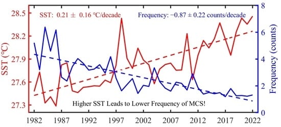
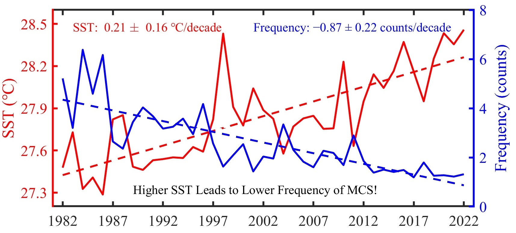
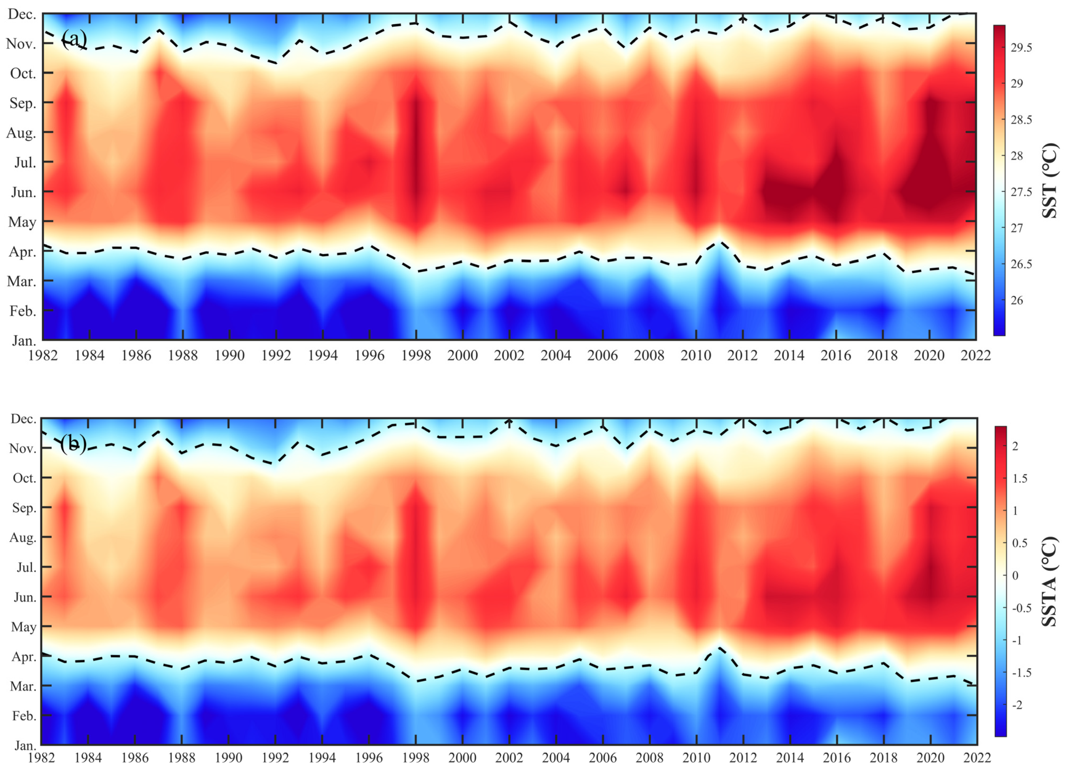
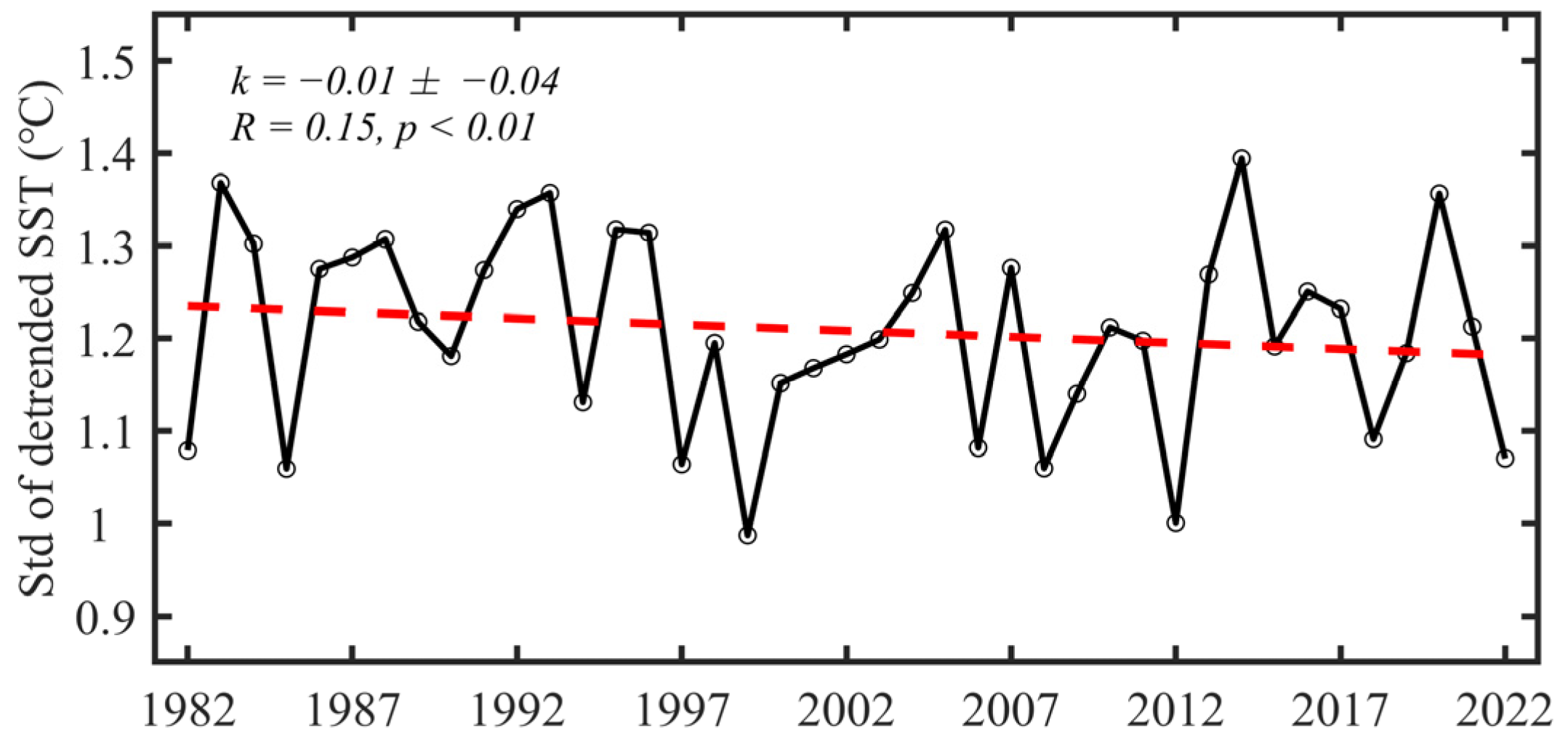
3.1. Spatial Distribution and Temporal Trends in SST and Its Variability

The climatological mean SST serves as the background condition for MCS occurrence, while the average 10th percentile threshold value indicates the maximum temperature for MCS appearance. Additionally, the standard deviation of detrended SST reflects the degree of temperature variability. Therefore, understanding the spatial distribution of these three physical quantities is crucial for comprehending the characteristics and trends of MCSs. To this end, Figure 3a–c depict the spatial distribution of the climatological mean SST, the 10th percentile SST (i.e., the threshold for computing MCSs), and the standard deviation of detrended SST from 1982 to 2022 in the SCS.

From Figure 3a, it is apparent that the climatological mean SST is influenced by the presence of land boundaries, resulting in a northeast–southwest trending distribution. The lowest average temperatures, approximately 22 °C, are observed near the Taiwan Strait in the northeastern part of the SCS, while the highest average SST, reaching around 29 °C, is found near the southern end of the Nansha Islands in the southwestern part of the SCS. The mean climatological temperature of the entire SCS stands at 27.85 ± 1.23 °C, with a median of 28.28 °C.

After removing annual cycles, the 10th percentile SST from 1982 to 2022 generally remains above 27 °C in most areas of the SCS, with the lowest values (approximately 20 °C) observed near the Taiwan Strait (Figure 3b). In the entire SCS, the average value of the 10th percentile SST is 26.85 ± 1.39 °C, with a median of 27.33 °C. Comparing the data in Figure 3a,b reveals that the average of the 10th percentile threshold is typically about 1 °C below the climatological mean. However, such temperature disparities are not uniform across the SCS. In the shallow coastal areas of the northwestern part of the SCS, differences are more pronounced close to the shore, while they diminish and in the southern regions of the sea, the deeper waters, and the southern regions of the sea.

The spatial variability is evident in Figure 3c, illustrating the standard deviations of detrended SST across the study period. These values depict the overall SST variability not explained by linear trends. Remarkably, the standard deviation exhibits significant spatial variation, with maximum values exceeding 4 °C observed in the shallow shelf regions of the northern SCS. In contrast, values in the southeastern SCS are less than 0.5 °C.

The annual variations in SSTAs, after removing the climatological mean (1982–2022), reflect the overall background temperature changes in the SCS. Previous studies suggest that with global warming, these anomalies are expected to increase annually. To verify this viewpoint and determine the specific rate of increase, Figure 4 illustrates the annual changes in SSTAs. In this study, we calculated the daily SSTAs relative to the seasonal climatology for each grid point. The current temporal trend of SSTAs is approximately 0.21 ± 0.16 °C/decade, as indicated by the red dashed line in Figure 4. This spatial trend is heterogeneous. In the Taiwan Strait and the coastal areas of the northeastern SCS, except for the Pearl River Estuary, the rate of increase in the northern Beibu Gulf area is significantly higher than in other regions, with maximum values exceeding 0.4 °C/decade. Notably, the SSTA values in 1998 are notably higher than in other years, likely influenced by the El Niño phenomenon. However, this aspect falls beyond the scope of the current study and will not be further discussed herein.

Based on the monthly SST (Figure 5a) and SSTA (Figure 5b) trends over time, it becomes apparent that the rise in SST mainly involves a prolongation of the period with higher temperatures. Specifically, the duration of time with temperatures exceeding 27.50 °C shifted from occurring between April and November in 1982 to spanning from March to December in 2022 (indicated by the dashed line in Figure 5a). The average temperature within the 27.50 °C isotherm gradually increased from 28.42 °C in 1982 to 28.99 °C in 2022, indicating a rise of 0.57 °C over the period. Similar conclusions can be drawn from the annual variation curve of SSTAs (Figure 5b). The range of the −0.50 °C SSTA contour shifted from approximately April to November in 1982 to March to December in 2022.

The variation in SST reflects the overall temperature trend in the SCS, while the temporal changes in the standard deviation of SST represent the degree of temperature variability. A higher value indicates greater temperature variability, larger fluctuations, and a higher likelihood of extreme temperatures., while a lower value indicates the opposite. From Figure 6, it is evident that the rate of change in the standard deviation of SST after removing the linear trend is −0.01 ± −0.04 °C/decade (p < 0.01). This observation is also supported by the trends observed in Figure 5a, where the variability in temperature decreases over time, leading to a corresponding decrease in variance.

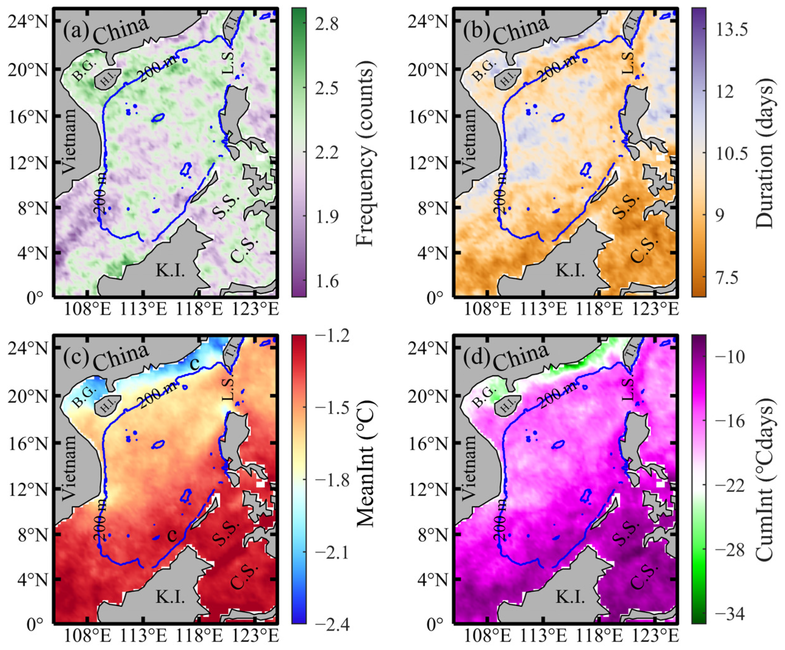
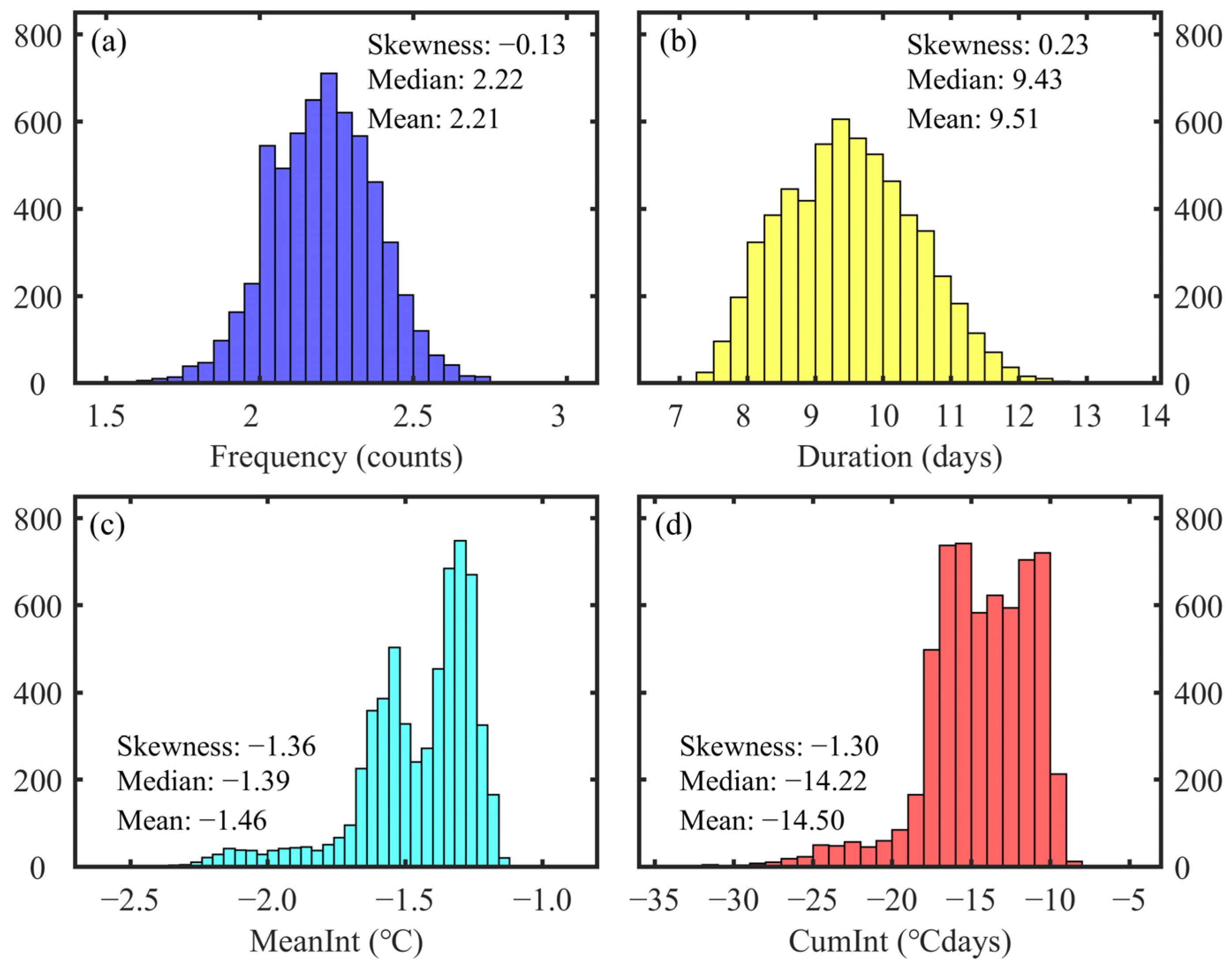
3.2. Spatial Distribution of MCS Characteristics

Figure 7 illustrates the annual average characteristics of MCSs in the SCS from 1982 to 2022, encompassing the spatial distribution of frequency (Figure 7a), duration (Figure 7b), mean intensity (Figure 7c), and cumulative intensity (Figure 7d). It is noteworthy that the annual values of MCS characteristics utilized in the subsequent analysis were derived by averaging these characteristics for each grid point annually. Particularly, from Figure 7a, it is evident that within the SCS region, the annual average frequency exhibits a spatially non-uniform distribution. Higher frequencies are observed in the Beibu Gulf area and the waters surrounding Hainan Island. Specifically, the maximum frequency occurs on the western side of Kalimantan Island (111.375°E, 3.125°N), reaching 2.81 counts/year, while the minimum value is observed southwest of the SCS (105.125°E, 3.125°N), with only 1.51 counts/year.

Comparing Figure 7a,b reveals that regions with high frequencies typically do not overlap with areas exhibiting prolonged durations of MCSs. For instance, many coastal areas in the northeastern region, where the MCS frequency is relatively low, exhibit higher durations (Figure 7b). The maximum duration of MCSs occurs in the nearshore waters of the northeastern part of the SCS (116.126°E, 22.875°N), reaching 14.01 days, while the minimum duration is observed in the southern part of the SCS (112.125°E, 3.875°N), with only 6.95 days. Furthermore, comparing Figure 3c and Figure 7c, it is evident that areas exhibiting high mean intensity correspond to regions with significant SST variability. Specifically, the strongest mean intensity is observed at (117.125°E, 22.875°N), reaching −2.47 °C, while the weakest intensity of only −1.12 °C is found at (114.125°E, 7.875°N). It is worth noting that the intensity of MCSs is represented by negative values; therefore, the smaller the numerical value (the bluer the color in Figure 7c), the greater the intensity of the MCS. The spatial distribution of MCS intensity exhibits a northeast-to-southwest directional pattern, similar to the spatial distribution of detrended SST variance in Figure 3c. Additionally, this directional pattern suggests a potential connection between MCS intensity and local SST variations.

Regarding the cumulative intensity of MCSs, it is known from its calculation formula that it results from the combined effects of duration (Figure 7b) and mean intensity (Figure 7c). As both of them exhibit enhanced distributions in the nearshore areas of the northern SCS, the cumulative intensity in coastal regions is notably higher than in open sea areas. The strongest cumulative intensity occurs at (115.625°E, 22.875°N), reaching −39.55 °C days, approximately three times higher than that in the central open sea of the SCS. Conversely, the weakest value is observed at (115.375°E, 8.125°N), only reaching −8.35 °C days (Figure 7d). This spatial distribution pattern underscores the influence of both duration and mean intensity on the cumulative intensity of MCSs, particularly in coastal regions, where both factors are prominently enhanced.

For a clearer understanding of the quantitative characteristics of MCSs in the SCS, Figure 8 presents the statistical histograms of the four attributes of MCSs. It is evident from the figure that the spatially averaged frequency of MCSs in the SCS region exhibits characteristics close to a normal distribution. The mean value is 2.21 counts/year, with a median of 2.22 counts/year, suggesting minimal skewness (−0.13) in the data distribution (Figure 8a). Similarly, the spatially averaged duration of MCSs in the SCS region also demonstrates characteristics close to a normal distribution (Figure 8b), with a mean value of 9.51 days and a median of 9.43 days. However, the average intensity of MCSs displays a noticeable skewed (0.23) distribution (Figure 8c). With a mean value of −1.46 °C and a median of −1.39 °C, it exhibits a skewness of −1.36. Likewise, influenced by the distribution of mean intensity of MCSs, the cumulative intensity also shows a skewed distribution. The mean value is −14.50 °C days, with a median of −14.22 °C days, resulting in a skewness of −1.30. This observation underscores the non-normal distribution characteristics of MCS intensity, suggesting a prevalence of certain extreme values in the dataset.

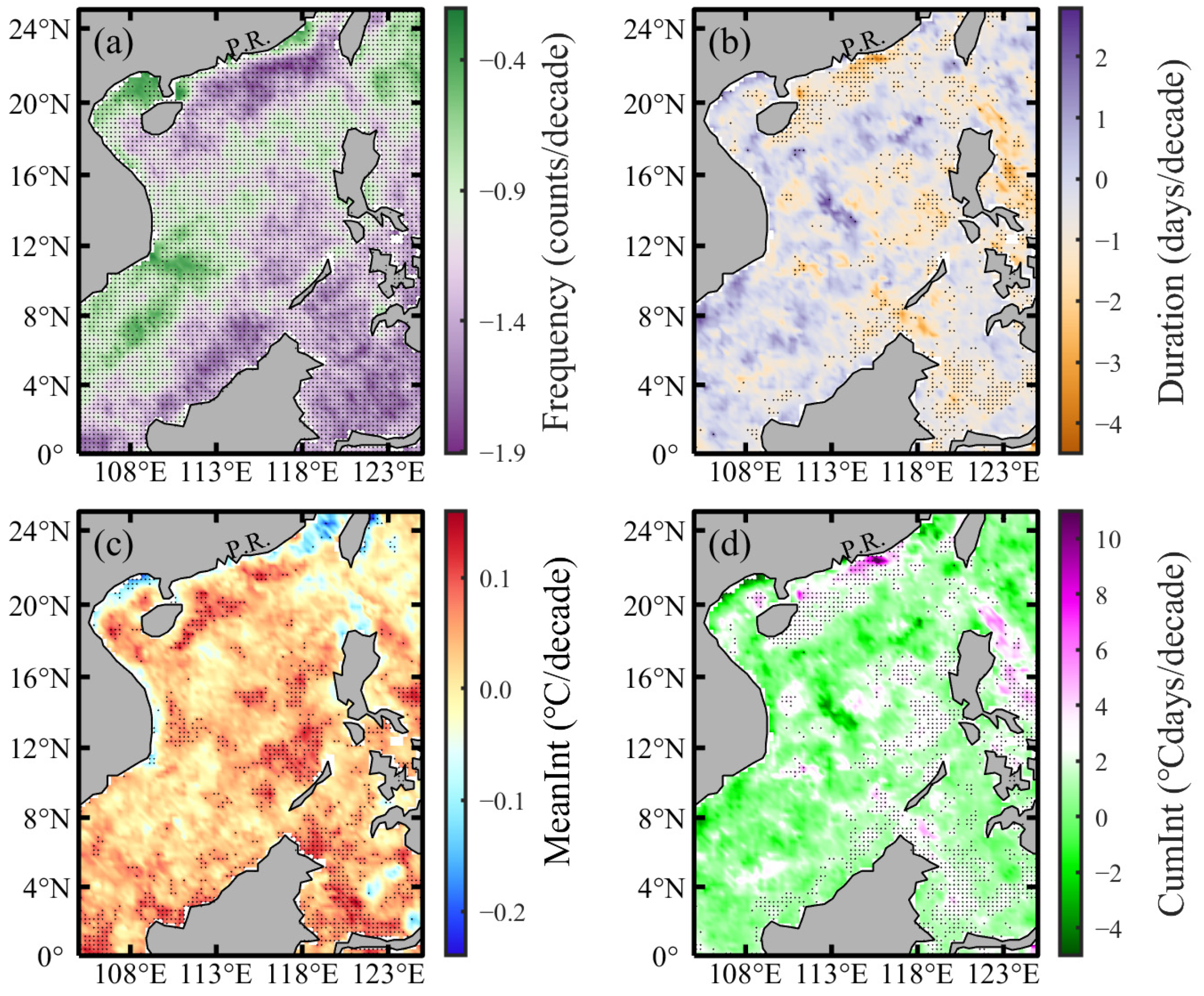
3.3. Spatial Distribution Trends of MCS Characteristics

Figure 9 illustrates the spatial distribution of the four characteristic trends of MCSs. Across the entire SCS, the comprehensive decreasing trend in frequency is evident, all of which pass the 95% confidence test (Figure 9a). The strongest negative trend in frequency is primarily observed in the northeastern part of the SCS, away from the coastal boundaries, decreasing at a rate of approximately −1.95 counts/decade. Conversely, the weakest negative trend in MCS frequency occurs in the Beibu Gulf area, decreasing at a rate of approximately −0.35 counts/decade. This comprehensive analysis underscores the regional disparities in frequency trends across the SCS, shedding light on the varied dynamics shaping MCS occurrence patterns in different geographical zones. The trend of MCS frequency exhibits a robust negative correlation with SSTAs, indicated by a Pearson correlation coefficient of −0.86, passing the 99% confidence test. However, there is no significant correlation between the trend of MCS frequency and SST standard deviation trends, with a correlation coefficient of only 0.11, failing to pass the 90% confidence test. This suggests that variations in MCS frequency are primarily driven by SST. Consequently, with further increases in SST, it is anticipated that the frequency of MCSs will continue to decrease.

The trend of duration differs in magnitude from that of frequency, exhibiting a spatial distribution characterized by alternating positive and negative values (Figure 9b). Regions with negative duration trends mostly pass the 95% confidence test, while positive trends mostly do not. Hence, the overall trend of duration should demonstrate a decrease. Moreover, significant declines in duration align with the most rapid decreases in frequency, especially near the nearshore areas in the northern part of the SCS. The region where duration decreases most rapidly is located near Pearl River Estuary, with a significant decline exceeding −2.67 °C days/decade (p < 0.05; Figure 9b). In contrast to the frequency, the duration of MCSs displays a negative correlation with SSTA trends, with a Pearson correlation coefficient of −0.45. Conversely, it demonstrates a positive correlation with changes in SST standard deviation, with a Pearson correlation coefficient of 0.32. Both correlations were verified with a 95% confidence test, indicating that variations in SST and its variance both impact the duration of MCSs.

Across the entire SCS region, a generally positive trend is observed in the mean intensity of MCSs (Figure 9c). Specifically, positive trends in the mean intensity are observed in the northeastern part of the SCS near the continental shelf areas, around Hainan Island, the western and the southern part of Luzon Island, and the eastern coastal areas of Vietnam, all of which pass the 95% confidence test. It is worth noting once more that MCS intensities are represented as negative values. Thus, a positive trend in the mean intensity over time indicates a weakening of MCSs. Additionally, the most significant weakening in the mean intensity is observed in the east of the Hainan Island region and the north of the Palawan Island region, reaching about 0.15 °C/decade. In the regions adjacent to the nearshore areas of the Beibu Gulf, the Taiwan Strait, and the coastal upwelling zones off the eastern coast of Vietnam, the most notable enhancement in the mean intensity is observed, with approximate values of about −0.15 °C/decade. Therefore, it is anticipated that the MCSs in these nearshore regions will progressively intensify in the future, with an expected increasingly conspicuous impact on marine ecosystems. The trends in MCS mean intensity exhibit weak Pearson correlations with the trends in SSTA and its standard deviation, with coefficients of −0.26 (p = 0.10) and −0.05 (p = 0.76), respectively. This suggests that the intensity of MCSs is not affected by changes in SST standard deviation.

The spatial distribution of cumulative intensity exhibits a pattern similar to that of duration, characterized by alternating positive and negative values (Figure 9d). However, regions where the rate of change in cumulative intensity is significant at 95% confidence typically coincide with positive-value regions. Combining Figure 9b,c reveals that these areas generally typically exhibit shorter duration and increased mean intensity, suggesting that future MCSs will be shorter-lived and more intense. The Pearson correlation coefficients between the trends in the cumulative intensity of MCSs and the trends in SSTAs and SST standard deviation are not high, with values of 0.29 (p = 0.07) and −0.28 (p = 0.07), respectively. This indicates the combined influence of MCS intensity and duration on the cumulative intensity of MCSs. Moreover, the observed trends suggest potential shifts in MCS dynamics, which could have implications for various environmental and ecological processes in the SCS. While this is an intriguing scientific question, it falls beyond the scope of the current study. Further investigation and discussion on this topic will be pursued in future research endeavors.

Similarly, to gain a clearer understanding of the numerical characteristics of MCSs in the SCS, Figure 10 provides statistical histograms for the trends in four characteristic variables. Overall, they exhibit characteristics of a normal distribution. The average change rate of frequency is −1.14 counts/decade, with a median of −1.16 counts/decade and a skewness of 0.26 (Figure 10a). The average change rate of duration is −0.57 days/decade, with a median of −0.59 days/decade and a skewness of −0.02 (Figure 10b). Among them, 20.27% of the data correspond to a positive trend in duration, but as indicated by Figure 9b, most of these data do not pass the 95% confidence test.

Examining the statistical histogram of mean intensity trends in Figure 10c, it is observed that the mean value of the intensity change rate is 0.02 °C/decade, with a median of 0.03 °C/decade and a skewness of −0.93. Approximately 75.54% of grid points correspond to positive values of the intensity change rate, and considering Figure 9c, most of these grid points pass the 95% confidence test. Given that the mean intensity of MCSs is negative, positive change rates indicate a weakening trend in the mean intensity.

Furthermore, from the statistical histogram of cumulative intensity trends in Figure 10d, it is observed that the mean value of cumulative intensity is 1.16 °C days/decade, with a median of 1.16 °C days/decade and a skewness of 0.18. Similarly, 82.87% of grid points exhibit positive values of the cumulative intensity change rate, and considering Figure 9d, it is noted that most of these points pass the 95% confidence test.

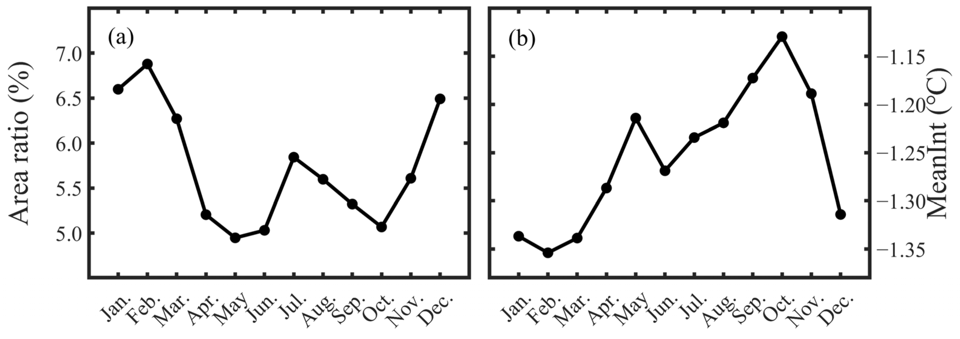
3.4. Seasonal Variations in Marine Cold Spells

Liu et al. [70], along with several other previous studies [71], indicate that the SST in the SCS is regulated by seasonal variations in upper ocean circulation, exhibiting significant seasonal cycles. Furthermore, MCSs exhibit noticeable seasonal variations in their adverse effects on marine life, with most instances of MCSs negatively impacting marine organisms occurring during the winter months [23]. Therefore, investigating the seasonal variations in MCSs holds significant scientific significance.

Figure 11 illustrates the climatological average area of the occurrence of MCSs (Figure 11a) and the monthly distribution of the average intensity in the SCS. The calculation formula for the area ratio is determined by dividing the total number of MCS occurrence points from 1982 to 2022 (with repeated points being counted each time they appear) by the total number of grid points in the SCS during this period. This method provides a quantitative measure of the spatial extent of MCS occurrences, facilitating a comprehensive analysis of their distribution patterns and temporal variations.

As depicted in Figure 11a, the occurrence area of MCSs is notably larger in winter than in summer. The peak occurrence area is observed in February, reaching 6.87% of the total grid points in the SCS over the 41 years under study. Conversely, the smallest area occurs in May, representing only 4.95% of the total grid points. Furthermore, it is worth noting that there is a noticeable increase in the proportion of MCS areas in July. This could be related to the observed decrease in SST around July in the SCS. From the perspective of the mean intensity, it is also observed that MCSs are more intense during the winter months. The most intense mean intensity occurs in February, reaching −1.35 °C. However, the weakest intensity does not occur in the summer months but rather in the subsequent autumn month of October, with a minimum intensity of only −1.13 °C. This observation highlights the seasonal variability in the intensity of MCSs, with winter months typically exhibiting stronger intensities compared to other seasons.

4. Discussion

4.1. Selection of Climate Baseline Periods

MCSs are commonly defined as extreme temperature occurrences within a specific climatic context, akin to MHWs. The identification of MCSs typically necessitates climatic data spanning at least 30 years, ensuring a comprehensive assessment of temperature anomalies over a significant timeframe. During the identification process, two main methods are employed: fixed climatic baseline periods and sliding climatic baseline periods. The former entails utilizing consistent climatic data throughout, irrespective of the year, which is suitable for studying marine organisms with limited environmental adaptability. Conversely, the latter incorporates data from 15 years before and after the year of MCS detection, aiming to represent genuine climatic conditions experienced by marine organisms.

While disparities between the two methods may not be noticeable for brief historical spans, caution is warranted when extending analyses to future periods. In particular, future scenario studies often extend discussions to 2100, where the influence of climate change, notably global warming, is evident. Notable disparities exist between climatic conditions of preceding and subsequent 30-year periods; hence, utilizing the fixed 30 years as the climatic baseline is suitable for studying marine organisms with sluggish temperature responses. However, for marine organisms with rapid temperature responses, the continued utilization of the fixed 30 years as the climatic baseline may not pose significant threats, resulting in reduced significance in MCS studies.

In summary, while both fixed and sliding baseline periods have advantages and disadvantages, caution is necessary when projecting future periods, especially when employing CMIP6 models for future scenario simulations, due to potential pronounced discrepancies between the two methods.

4.2. Mechanisms of MCS Formation

From the expression of the oceanic heat budget equation, it is apparent that several factors contribute to the formation of MCSs. These factors include thermodynamic forcing from the atmosphere, such as a decrease in local air temperature directly leading to the loss of SST. Dynamic forcing from the atmosphere, for instance, leads to an increase in local wind speed, which enhances mixing, thereby bringing cold water from the lower layers to the surface and causing a reduction in SST. Anomalies in oceanic advection occur when there is a decrease in heat transported from the horizontal sides into the area or an increase in heat transported out of the area, resulting in a decrease in the net heat content of the area. Furthermore, the strengthening of local upwelling results in an excess of cold water reaching the upper layers, consequently causing a decrease in SST [11]. Additionally, there may be some other unknown oceanic processes that can induce the generation of MCSs.

It is evident that diagnosing and analyzing the mechanism of MCS generation requires the utilization of various atmospheric elements and three-dimensional oceanic data. However, using only the SST data in this study does not allow for the diagnosis and analysis of the complex processes mentioned above. Relevant work will be undertaken in future research endeavors.

5. Conclusions

Marine cold spells, known as extreme ocean temperature events, carry significant ecological and societal implications, garnering attention in both regional and species-specific research. These events cause disruptions in marine ecosystems, leading to widespread impacts, including mass fish and invertebrate deaths, population declines, coral bleaching, changes in species distribution, and shifts in phenology. Amid ongoing global oceanic transformations, MCSs may act as barriers to the spread of non-native or invasive species, potentially offering refuge for cold-adapted local taxa and modifying ecosystem structure and functionality. Given their dual roles in shaping marine ecosystems and implications for societal needs, identifying the timing and locations of prolonged MCS occurrences and understanding their future changes is crucial for effectively managing and safeguarding marine resources.

To address these concerns, our study explores the spatial distribution and variability of SST from 1982 to 2022 while simultaneously assessing alterations in means and trends among MCSs during this period. We examined annual variations in SSTs to understand the background conditions for MCS occurrence. Spatially, the climatological mean SST ranges from approximately 22 °C near the Taiwan Strait to around 29 °C near the Nansha Islands, with an average of 27.85 ± 1.23 °C across the SCS. Notable variations exist in the 10th percentile SST, generally remaining above 27 °C, while standard deviation values exhibit significant spatial discrepancies, exceeding 4 °C in northern shelf regions and remaining below 0.5 °C in the southeastern SCS.

Annual SSTAs, reflecting background temperature changes, were examined to assess the impact of global warming, revealing a heterogeneous spatial trend of approximately 0.21 ± 0.16 °C/decade across the SCS. Over time, the monthly SST and SSTA data reveal a prolonged period of higher temperatures in the SCS, with temperatures exceeding 27.50 °C transitioning from April to November in 1982 to March to December in 2022. Correspondingly, the average temperature within the 27.50 °C isotherm rises from 28.42 °C to 28.99 °C, indicating a 0.57 °C increase over the period. Similarly, the range of the −0.50 °C SSTA contour shifted from approximately April to November in 1982 to March to December in 2022. The declining standard deviation of SST in the SCS indicates reduced temperature variability over time.

The annual average characteristics of MCSs in the SCS from 1982 to 2022 reveal spatial non-uniformity in frequency, with higher values near the Beibu Gulf and Hainan Island. Conversely, longer durations are observed in the coastal areas of the northeastern region. The mean intensity displays a skewed distribution, influenced by SST variability, while cumulative intensity is notably higher in coastal regions due to enhanced factors. Statistical histograms depict characteristics close to a normal distribution for frequency and duration but skewness for intensity and cumulative intensity, indicating a prevalence of extreme values.

The analysis reveals a comprehensive decrease in MCS frequency across the SCS, with the strongest decline observed in the northeast. Trends in duration vary, with some areas showing decreases, notably near the Pearl River Estuary. The mean intensity generally weakens, particularly in certain regions, while cumulative intensity trends fluctuate, aligning with duration and mean intensity patterns. Statistical histograms indicate normal distributions for frequency and duration trends, while the mean and cumulative intensity trends skew toward positive values, implying weakening MCSs overall. Winter months in the SCS exhibit larger MCS occurrence areas, peaking in February and displaying higher mean intensities compared to other seasons. However, the weakest intensity is observed in October, indicating seasonal variability in MCS intensity.

Our study represents an attempt to quantify and compare long-term trends in MCSs in the SCS. These findings serve as a roadmap for policymakers and managers, providing insight into the locations and extent of MCS exposure in the ocean and the evolving nature of this exposure over time.

References

1. IPCC. Summary for policymakers. In Climate Change 2021: The Physical Science Basis; Contribution of Working Group I to the Sixth Assessment Report of the Intergovernmental Panel on Climate Change; Cambridge University Press: Cambridge, UK, 2021; Available online: https://www.ipcc.ch/report/ar6/wg1/chapter/summary-for-policymakers/ (accessed on 25 March 2024).
2. Drijfhout, S.; Bathiany, S.; Beaulieu, C.; Brovkin, V.; Claussen, M.; Huntingford, C.; Scheffer, M.; Sgubin, G.; Swingedouw, D. Catalogue of abrupt shifts in Intergovernmental Panel on Climate Change climate models. Proc. Natl. Acad. Sci. USA 2015, 112, E5777–E5786. [Google Scholar] [CrossRef]
3. Schlegel, R.W.; Darmaraki, S.; Benthuysen, J.A.; Filbee-Dexter, K.; Oliver, E.C. Marine cold-spells. Prog. Oceanogr. 2021, 198, 102684. [Google Scholar] [CrossRef]
4. Wang, Y.; Kajtar, J.B.; Alexander, L.V.; Pilo, G.S.; Holbrook, N.J. Understanding the changing nature of marine cold-spells. Geophys. Res. Lett. 2022, 49, e2021GL097002. [Google Scholar] [CrossRef]
5. Hurst, T.P. Causes and consequences of winter mortality in fishes. J. Fish Biol. 2007, 71, 315–345. [Google Scholar] [CrossRef]
6. González-Espinosa, P.; Donner, S. Predicting cold-water bleaching in corals: Role of temperature, and potential integration of light exposure. Mar. Ecol. Prog. Ser. 2020, 642, 133–146. [Google Scholar] [CrossRef]
7. Barlas, M.E.; Deutsch, C.J.; de Wit, M.; Ward-Geiger, L.I. Florida Manatee Cold-Related Unusual Mortality Event, January–April 2010; Final Report to USFWS (grant 40181AG037); Florida Fish and Wildlife Conservation Commission: St. Petersburg, FL, USA, 2011; p. 138. Available online: https://downloads.regulations.gov/FWS-R4-ES-2015-0178-3824/content.pdf (accessed on 25 March 2024).
8. Cavanaugh, K.C.; Kellner, J.R.; Forde, A.J.; Gruner, D.S.; Parker, J.D.; Rodriguez, W.; Feller, I.C. Poleward expansion of mangroves is a threshold response to decreased frequency of extreme cold events. Proc. Natl. Acad. Sci. USA 2013, 111, 723–727. [Google Scholar] [CrossRef]
9. Pecl, G.T.; Araújo, M.B.; Bell, J.D.; Blanchard, J.; Bonebrake, T.C.; Chen, I.-C.; Clark, T.D.; Colwell, R.K.; Danielsen, F.; Evengård, B.; et al. Biodiversity redistribution under climate change: Impacts on ecosystems and human well-being. Science 2017, 355, eaai9214. [Google Scholar] [CrossRef]
10. Chiswell, S.M. Global trends in marine heatwaves and cold spells: The impacts of fixed versus changing baselines. J. Geophys. Res. Oceans 2022, 127, e2022JC018757. [Google Scholar] [CrossRef]
11. Yao, Y.; Wang, C.; Fu, Y. Global marine heatwaves and cold-spells in present climate to future projections. Earth’s Futur. 2022, 10, e2022EF002787. [Google Scholar] [CrossRef]
12. Dalsin, M.; Walter, R.K.; Mazzini, P.L.F. Effects of basin-scale climate modes and upwelling on nearshore marine heatwaves and cold spells in the California Current. Sci. Rep. 2023, 13, 12389. [Google Scholar] [CrossRef]
13. Ciappa, A.C. Effects of Marine Heatwaves (MHW) and Cold Spells (MCS) on the surface warming of the Mediterranean Sea from 1989 to 2018. Prog. Oceanogr. 2022, 205, 102828. [Google Scholar] [CrossRef]
14. Schopmeyer, S.A.; Lirman, D.; Bartels, E.; Byrne, J.; Gilliam, D.S.; Hunt, J.; Johnson, M.E.; Larson, E.A.; Maxwell, K.; Nedimyer, K.; et al. In situ coral nurseries serve as genetic repositories for coral reef restoration after an extreme cold-water event. Restor. Ecol. 2011, 20, 696–703. [Google Scholar] [CrossRef]
15. Nielsen, J.J.V.; Kenkel, C.D.; Bourne, D.G.; Despringhere, L.; Mocellin, V.J.L.; Bay, L.K. Physiological effects of heat and cold exposure in the common reef coral Acropora millepora. Coral Reefs 2020, 39, 259–269. [Google Scholar] [CrossRef]
16. Yuan, D. Dynamics of the cold-water event off the southeast coast of the United States in the summer of 2003. J. Phys. Oceanogr. 2006, 36, 1912–1927. [Google Scholar] [CrossRef]
17. Chang, Y.; Lee, M.-A.; Lee, K.-T.; Shao, K.-T. Adaptation of fisheries and mariculture management to extreme oceanic environmental changes and climate variability in Taiwan. Mar. Policy 2013, 38, 476–482. [Google Scholar] [CrossRef]
18. Lee, M.-A.; Yang, Y.-C.; Shen, Y.-L.; Chang, Y.; Tsai, W.-S.; Lan, K.-W.; Kuo, Y.-C. Effects of an unusual cold-water intrusion in 2008 on the catch of coastal fishing methods around Penghu Islands, Taiwan. Terr. Atmos. Ocean. Sci. 2014, 25, 107–120. [Google Scholar] [CrossRef]
19. Colella, M.A.; Ruzicka, R.R.; Kidney, J.A.; Morrison, J.M.; Brinkhuis, V.B. Cold-water event of January 2010 results in catastrophic benthic mortality on patch reefs in the Florida Keys. Coral Reefs 2012, 31, 621–632. [Google Scholar] [CrossRef]
20. Roberts, K.; Collins, J.; Paxton, C.H.; Hardy, R.; Downs, J. Weather patterns associated with green turtle hypothermic stunning events in St. Joseph Bay and Mosquito Lagoon, Florida. Phys. Geogr. 2014, 35, 134–150. [Google Scholar] [CrossRef]
21. Pirhalla, D.E.; Sheridan, S.C.; Ransibrahmanakul, V.; Lee, C.C. Assessing cold-snap and mortality events in south Florida coastal ecosystems: Development of a biological cold stress index using satellite SST and weather pattern forcing. Estuaries Coasts 2014, 38, 2310–2322. [Google Scholar] [CrossRef]
22. Lirman, D.; Schopmeyer, S.; Manzello, D.; Gramer, L.J.; Precht, W.F.; Muller-Karger, F.; Banks, K.; Barnes, B.; Bartels, E.; Bourque, A.; et al. Severe 2010 cold-water event caused unprecedented mortality to corals of the Florida reef tract and reversed previous survivorship patterns. PLoS ONE 2011, 6, e23047. [Google Scholar] [CrossRef]
23. Hsieh, H.J.; Hsien, Y.L.; Jeng, M.S.; Tsai, W.S.; Su, W.C.; Chen, C.A. Tropical fishes killed by the cold. Coral Reefs 2008, 27, 599. [Google Scholar] [CrossRef]
24. Lotterhos, K.E.; Markel, R.W. Oceanographic drivers of offspring abundance may increase or decrease reproductive variance in a temperate marine fish. Mol. Ecol. 2012, 21, 5009–5026. [Google Scholar] [CrossRef]
25. Bennett, S.; Duarte, C.M.; Marbà, N.; Wernberg, T. Integrating within-species variation in thermal physiology into climate change ecology. Philos. Trans. R. Soc. B Biol. Sci. 2019, 374, 20180550. [Google Scholar] [CrossRef] [PubMed]
26. Donders, T.H.; de Boer, H.J.; Finsinger, W.; Grimm, E.C.; Dekker, S.C.; Reichart, G.J.; Wagner-Cremer, F. Impact of the Atlantic Warm Pool on precipitation and temperature in Florida during North Atlantic cold spells. Clim. Dyn. 2009, 36, 109–118. [Google Scholar] [CrossRef]
27. Campbell-Staton, S.C.; Cheviron, Z.A.; Rochette, N.; Catchen, J.; Losos, J.B.; Edwards, S.V. Winter storms drive rapid phenotypic, regulatory, and genomic shifts in the green anole lizard. Science 2017, 357, 495–498. [Google Scholar] [CrossRef]
28. Schlegel, R.W.; Oliver, E.C.; Wernberg, T.; Smit, A.J. Nearshore and offshore co-occurrence of marine heatwaves and cold-spells. Prog. Oceanogr. 2017, 151, 189–205. [Google Scholar] [CrossRef]
29. Tuckett, C.A.; Wernberg, T. High latitude corals tolerate severe cold spell. Front. Mar. Sci. 2018, 5, 14. [Google Scholar] [CrossRef]
30. Yao, Y.; Wang, C. Marine heatwaves and cold-spells in global coral reef zones. Prog. Oceanogr. 2022, 209, 102920. [Google Scholar] [CrossRef]
31. Zuo, X.; Su, F.; Wu, W.; Chen, Z.; Shi, W. Spatial and temporal variability of thermal stress to China’s coral reefs in South China Sea. Chin. Geogr. Sci. 2015, 25, 159–173. [Google Scholar] [CrossRef]
32. Sun, W.; Dong, C.; Tan, W.; Liu, Y.; He, Y.; Wang, J. Vertical structure anomalies of oceanic eddies and eddy-induced transports in the South China Sea. Remote Sens. 2018, 10, 795. [Google Scholar] [CrossRef]
33. Yao, Y.; Wang, C. Variations in summer marine heatwaves in the South China Sea. J. Geophys. Res. Oceans 2021, 126, e2021JC017792. [Google Scholar] [CrossRef]
34. Sun, W.; Zhou, S.; Yang, J.; Gao, X.; Ji, J.; Dong, C. Artificial intelligence forecasting of marine heatwaves in the South China Sea using a combined U-Net and ConvLSTM system. Remote Sens. 2023, 15, 4068. [Google Scholar] [CrossRef]
35. Zhuang, W.; Xie, S.; Wang, D.; Taguchi, B.; Aiki, H.; Sasaki, H. Intraseasonal variability in sea surface height over the South China Sea. J. Geophys. Res. Oceans 2010, 115, C04010. [Google Scholar] [CrossRef]
36. Shu, Y.; Wang, Q.; Zu, T. Progress on shelf and slope circulation in the northern South China Sea. Sci. China Earth Sci. 2018, 61, 560–571. [Google Scholar] [CrossRef]
37. Zhu, Y.; Sun, J.; Wang, Y.; Li, S.; Xu, T.; Wei, Z.; Qu, T. Overview of the multi-layer circulation in the South China Sea. Prog. Oceanogr. 2019, 175, 171–182. [Google Scholar] [CrossRef]
38. Geng, B.; Xiu, P.; Liu, N.; He, X.; Chai, F. Biological response to the interaction of a mesoscale eddy and the river plume in the northern South China Sea. J. Geophys. Res. Oceans 2021, 126, e2021JC017244. [Google Scholar] [CrossRef]
39. Sun, W.; Liu, Y.; Chen, G.; Tan, W.; Lin, X.; Guan, Y.; Dong, C. Three-dimensional properties of mesoscale cyclonic warm-core and anticyclonic cold-core eddies in the South China Sea. Acta Oceanol. Sin. 2021, 40, 17–29. [Google Scholar] [CrossRef]
40. Mao, H.; Qi, Y.; Qiu, C.; Luan, Z.; Wang, X.; Cen, X.; Yu, L.; Lian, S.; Shang, X. High-resolution observations of upwelling and front in Daya Bay, South China Sea. J. Mar. Sci. Eng. 2021, 9, 657. [Google Scholar] [CrossRef]
41. Jiang, Y.; Zhang, W.; Wang, H.; Zhang, X. Assessing the spatio-temporal features and mechanisms of symmetric instability activity probability in the central part of the South China Sea based on a regional ocean model. J. Mar. Sci. Eng. 2023, 11, 431. [Google Scholar] [CrossRef]
42. Wu, M.; Xue, H.; Chai, F. Asymmetric chlorophyll responses enhanced by internal waves near the Dongsha Atoll in the South China Sea. J. Oceanol. Limnol. 2023, 41, 418–426. [Google Scholar] [CrossRef]
43. Qu, T.; Mitsudera, H.; Yamagata, T. Intrusion of the North Pacific waters into the South China Sea. J. Geophys. Res. Atmos. 2000, 105, 6415–6424. [Google Scholar] [CrossRef]
44. Qu, T.; Kim, Y.Y.; Yaremchuk, M.; Tozuka, T.; Ishida, A.; Yamagata, T. Can Luzon Strait transport play a role in conveying the impact of ENSO to the South China Sea? J. Clim. 2004, 17, 3644–3657. [Google Scholar] [CrossRef]
45. Qu, T.; Du, Y.; Meyers, G.; Ishida, A.; Wang, D. Connecting the tropical Pacific with Indian Ocean through South China Sea. Geophys. Res. Lett. 2005, 32, L24609. [Google Scholar] [CrossRef]
46. Qu, T.; Du, Y.; Sasaki, H. South China Sea throughflow: A heat and freshwater conveyor. Geophys. Res. Lett. 2006, 33, L23617. [Google Scholar] [CrossRef]
47. Yihui, D.; Chongyin, L.; Yanju, L. Overview of the South China sea monsoon experiment. Adv. Atmospheric Sci. 2004, 21, 343–360. [Google Scholar] [CrossRef]
48. Wang, G.; Ling, Z.; Wang, C. Influence of tropical cyclones on seasonal ocean circulation in the South China Sea. J. Geophys. Res. Atmos. 2009, 114, C10022. [Google Scholar] [CrossRef]
49. Kajikawa, Y.; Wang, B. Interdecadal change of the South China Sea summer monsoon onset. J. Clim. 2012, 25, 3207–3218. [Google Scholar] [CrossRef]
50. Cai, R.; Tan, H.; Qi, Q. Impacts of and adaptation to inter-decadal marine climate change in coastal China seas. Int. J. Clim. 2015, 36, 3770–3780. [Google Scholar] [CrossRef]
51. Li, Y.; Ren, G.; Wang, Q.; Mu, L.; Niu, Q. Marine heatwaves in the South China Sea: Tempo-Spatial pattern and its association with Large-Scale circulation. Remote Sens. 2022, 14, 5829. [Google Scholar] [CrossRef]
52. Liu, K.; Xu, K.; Zhu, C.; Liu, B. Diversity of marine heatwaves in the South China Sea regulated by ENSO phase. J. Clim. 2022, 35, 877–893. [Google Scholar] [CrossRef]
53. Mo, S.; Chen, T.; Chen, Z.; Zhang, W.; Li, S. Marine heatwaves impair the thermal refugia potential of marginal reefs in the northern South China Sea. Sci. Total. Environ. 2022, 825, 154100. [Google Scholar] [CrossRef] [PubMed]
54. Wang, Q.; Zhang, B.; Zeng, L.; He, Y.; Wu, Z.; Chen, J. Properties and drivers of marine heat waves in the northern South China Sea. J. Phys. Oceanogr. 2022, 52, 917–927. [Google Scholar] [CrossRef]
55. Han, T.; Xu, K.; Wang, L.; Liu, B.; Tam, C.-Y.; Liu, K.; Wang, W. Extremely long-lived marine heatwave in South China Sea during summer 2020: Combined effects of the seasonal and intraseasonal variations. Glob. Planet. Chang. 2023, 230, 104261. [Google Scholar] [CrossRef]
56. Song, Q.; Yao, Y.; Wang, C. Response of future summer marine heatwaves in the South China Sea to enhanced western pacific subtropical high. Geophys. Res. Lett. 2023, 50, e2023GL103667. [Google Scholar] [CrossRef]
57. Wang, Y.; Zhang, C.; Tian, S.; Chen, Q.; Li, S.; Zeng, J.; Wei, Z.; Xie, S. Seasonal cycle of marine heatwaves in the northern South China Sea. Clim. Dyn. 2023, 61, 3367–3377. [Google Scholar] [CrossRef]
58. Liu, S.; Lao, Q.; Zhou, X.; Jin, G.; Chen, C.; Chen, F. Impacts of marine heatwave events on three distinct upwelling systems and their implications for marine ecosystems in the Northwestern South China Sea. Remote Sens. 2023, 16, 131. [Google Scholar] [CrossRef]
59. Reynolds, R.W.; Smith, T.M.; Liu, C.; Chelton, D.B.; Casey, K.S.; Schlax, M.G. Daily high-resolution-blended analyses for sea surface temperature. J. Clim. 2007, 20, 5473–5496. [Google Scholar] [CrossRef]
60. Banzon, V.; Smith, T.M.; Chin, T.M.; Liu, C.; Hankins, W. A long-term record of blended satellite and in situ sea-surface temperature for climate monitoring, modeling and environmental studies. Earth Syst. Sci. Data 2016, 8, 165–176. [Google Scholar] [CrossRef]
61. Huang, B.; Liu, C.; Banzon, V.; Freeman, E.; Graham, G.; Hankins, B.; Smith, T.; Zhang, H.-M. Improvements of the Daily Optimum Interpolation Sea Surface Temperature (DOISST) Version 2.1. J. Clim. 2021, 34, 2923–2939. [Google Scholar] [CrossRef]
62. A Benthuysen, J.; A Smith, G.; Spillman, C.M.; Steinberg, C.R. Subseasonal prediction of the 2020 Great Barrier Reef and Coral Sea marine heatwave. Environ. Res. Lett. 2021, 16, 124050. [Google Scholar] [CrossRef]
63. Holbrook, N.J.; Hernaman, V.; Koshiba, S.; Lako, J.; Kajtar, J.B.; Amosa, P.; Singh, A. Impacts of marine heatwaves on tropical western and central Pacific Island nations and their communities. Glob. Planet. Chang. 2021, 208, 103680. [Google Scholar] [CrossRef]
64. Hobday, A.J.; Alexander, L.V.; Perkins, S.E.; Smale, D.A.; Straub, S.C.; Oliver, E.C.J.; Benthuysen, J.A.; Burrows, M.T.; Donat, M.G.; Feng, M.; et al. A hierarchical approach to defining marine heatwaves. Prog. Oceanogr. 2016, 141, 227–238. [Google Scholar] [CrossRef]
65. Holbrook, N.J.; Gupta, A.S.; Oliver, E.C.J.; Hobday, A.J.; Benthuysen, J.A.; Scannell, H.A.; Smale, D.A.; Wernberg, T. Keeping pace with marine heatwaves. Nat. Rev. Earth Environ. 2020, 1, 482–493. [Google Scholar] [CrossRef]
66. Oliver, E.C.; Benthuysen, J.A.; Darmaraki, S.; Donat, M.G.; Hobday, A.J.; Holbrook, N.J.; Schlegel, R.W.; Gupta, A.S. Marine Heatwaves. Annu. Rev. Mar. Sci. 2021, 13, 313–342. [Google Scholar] [CrossRef] [PubMed]
67. Jacox, M.G. Marine heatwaves in a changing climate. Nature 2019, 571, 485–487. [Google Scholar] [CrossRef]
68. Chiswell, S.M. Atmospheric wavenumber-4 driven South Pacific marine heat waves and marine cool spells. Nat. Commun. 2021, 12, 4779. [Google Scholar] [CrossRef]
69. Zhao, Z.; Marin, M. A MATLAB toolbox to detect and analyze marine heatwaves. J. Open Source Softw. 2019, 4, 1124. [Google Scholar] [CrossRef]
70. Liu, Z.; Yang, H.; Liu, Q. Regional dynamics of seasonal variability in the South China Sea. J. Phys. Oceanogr. 2001, 31, 272–284. [Google Scholar] [CrossRef]
71. Xie, S.; Xie, Q.; Wang, D.; Liu, W.T. Summer upwelling in the South China Sea and its role in regional climate variations. J. Geophys. Res. Oceans 2003, 108, 3261. [Google Scholar] [CrossRef]
Figure 1. Topography of the South China Sea. Shading indicates water depth (units: m), with the black contour representing the 200 m isobath. Geographical locations are abbreviated as B.G. for Beibu Gulf, H.I. for Hainan Island, P.R. for Pearl River Estuary, T.S. for Taiwan Strait, T.I. for Taiwan Island, L.S. for Luzon Strait, L.I. for Luzon Island, X.I. for Xisha Islands, Z.I. for Zhongsha Islands, N.I. for Nansha Islands, M.S. for Mindoro Strait, P.I. for Palawan Island, K.I. for Kalimantan Island, S.S. for Sulu Sea, and C.S. for Celebes Sea.
Remotesensing 16 01171 g001
Figure 2. Schematic representation of marine cold spells at an arbitrary point (115.125°E, 12.125°N) in the South China Sea during 2018. The black curve denotes sea surface temperature, the blue curve indicates the climatological average temperature from 1982 to 2022, and the green curve represents the threshold curve for marine cold spell determination. “MCS1” and “MCS2” represent two instances of marine cold spell events during the specified period.
Remotesensing 16 01171 g002
Figure 3. Climatological sea surface temperature from 1982 to 2022 (a), the 10th percentile sea surface temperature (indicating the threshold for defining marine cold spells) (b), and the spatial distribution of standard deviation of detrended sea surface temperature (c) in the South China Sea. The blue curve represents the 200 m isobath, while the meanings of the abbreviated letters correspond to those in Figure 1.
Remotesensing 16 01171 g003
Figure 4. Annual variation trend of the sea surface temperature anomalies averaged over the South China Sea, after removing the climatological mean (1982–2022). The black curve represents the annual mean SST anomalies, while the red dashed line indicates the results after linear regression fitting; “k” represents the slope of the fitted line (units: °C/decade), “R” indicates the coefficient of determination, and “p” denotes the significance level.
Remotesensing 16 01171 g004
Figure 5. Temporal evolution of sea surface temperature (a) and sea surface temperature anomalies (b). In panel (a), the black dashed lines represent the contour lines of 27.50 °C, while in panel (b), the black dashed lines represent the contour lines of −0.50 °C.
Remotesensing 16 01171 g005
Figure 6. Temporal trend of detrended mean sea surface temperature standard deviation in the South China Sea from 1982 to 2022 (units: °C/decade); “k” represents the slope of the fitted line (units: °C/decade), “R” indicates the coefficient of determination, and “p” denotes the significance level.
Remotesensing 16 01171 g006
Figure 7. Spatial distribution of the MCS frequency ((a), units: counts), duration ((b), units: days), mean intensity ((c), units: °C), and cumulative intensity ((d), units: °C days) of marine cold spells from 1982 to 2022. The blue line represents the 200 m isobath, and the meanings of the abbreviated letters are the same as in Figure 1.
Remotesensing 16 01171 g007
Figure 8. Statistical histograms of the MCS frequency ((a), units: counts), duration ((b), units: days), mean intensity ((c), units: °C), and cumulative intensity ((d), units: °C days) of marine cold spells in the South China Sea region from 1982 to 2022.
Remotesensing 16 01171 g008
Figure 9. Trends in characteristics of marine cold spells in the SCS between 1982 and 2022, specifically, (a) frequency (units: counts/decade), (b) duration (units: days/decade), (c) mean intensity (units: °C/decade), and (d) cumulative intensity (units: °C days/decade). In all subplots, black dots indicate trends that exceed the 95% confidence test (p <= 0.05). P.R. is the abbreviation for the Pearl River Estuary.
Remotesensing 16 01171 g009
Figure 10. Statistical histograms of the trends in frequency ((a), units: counts/decade), duration ((b), units: days/decade), mean intensity ((c), units: °C/decade), and cumulative intensity ((d), units: °C days/decade) of marine cold spells in the South China Sea from 1982 to 2022.
Remotesensing 16 01171 g010
Figure 11. Seasonal variations in the area ratio (a) and mean intensity (b) of marine cold spells in the South China Sea.
Remotesensing 16 01171 g011
Disclaimer/Publisher’s Note: The statements, opinions and data contained in all publications are solely those of the individual author(s) and contributor(s) and not of MDPI and/or the editor(s). MDPI and/or the editor(s) disclaim responsibility for any injury to people or property resulting from any ideas, methods, instructions or products referred to in the content.