Optical Imaging Method of Synthetic-Aperture Radar for Moving Targets

Abstract

Traditional synthetic-aperture radar (SAR) imaging, while adept at capturing stationary scenes with clarity, often results in the blurring of moving targets due to Doppler spectrum disparities. To overcome this, this study introduces an innovative optical approach for imaging moving targets. By employing a spatial light modulator (SLM), the phase information of SAR data can be modulated onto a light beam. Then, the light propagation path is meticulously designed to take advantage of the free propagation of light to compensate for the phase differences in SAR data, thereby achieving focal clarity. Simulations and experimental validations have demonstrated that this method surpasses traditional digital imaging techniques in terms of focusing precision. Additionally, the processing delay is only as long as the time taken for light propagation. The optical path is simple, avoiding complex assembly and alignment. This novel approach opens up new possibilities for the SAR imaging of moving targets, offering potential applications in moving target extraction, separation, and velocity estimation.

1. Introduction

Synthetic-aperture radar (SAR) constitutes an active observation system, offering versatile all-day and all-weather imaging capabilities. Its wide range of applications includes geological exploration, agricultural monitoring, terrain mapping, etc. [1,2,3,4,5,6,7,8,9]. Take geological exploration as an example; SAR is invaluable for its ability to map and analyze Earth’s subsurface structures with precision. Its penetrating radar waves enable the detection of geological features, such as faults and mineral deposits, hidden beneath the surface, offering a vital tool for resource exploration and disaster management. For instance, SAR sensors possess the capacity to detect subtle changes in terrain inclination due to adverse geological formations and can furnish early warning signals of impending collapse several days before a landslide [1]. The adaptability of SAR extends to various moving platforms, such as aircraft and satellites. By emitting pulses from diverse positions based on the motion of the platform, SAR generates the pulse repetition interval (PRI), which indicates the time interval between two emitted pulses. In SAR, utilizing the relative motion between the radar and the target leads to the formation of a synthetic aperture, thereby enhancing azimuth (parallel to the radar’s motion direction) resolution. Achieving high resolution in the range direction, perpendicular to the radar’s motion, involves the use of transmitted pulse signals, usually as linear frequency modulation signals. Echo data from SAR typically exist in a complex format and are stored in a two-dimensional matrix, where each row encapsulates the echo of an emitted pulse. The purpose of imaging is to reconstruct the backscattering information of the target from the collected data. Given the known nature of the transmitted signal, focusing in the range direction is relatively straightforward and can be achieved using a matched filter. However, the challenge lies in azimuth direction focusing, primarily owing to the complexity of range migration.

Various classical SAR imaging algorithms have been developed [10], including the matched filter [11], back projection [12], range Doppler [13], chirp scaling [14], and frequency scaling algorithms [15]. However, these algorithms were primarily designed for stationary scenes, which causes the images of moving targets to shift and become defocused, ultimately resulting in degraded imaging results [16]. In terms of the matched filter algorithm, it is designed following the maximum signal-to-noise ratio criterion and constructs a reference function which is conjugate matching with the phase of the echo data. Since the algorithm assumes a stationary target when constructing the signal model, the movement of targets in real scenarios can cause mismatch of the matched filter, which may affect the imaging accuracy. However, if the motion effects of the target are taken into account and the filter is redesigned accordingly, the imaging results can be improved [17]. In practical applications, individuals frequently possess prior knowledge of stationary scenes; however, their main interest lies in accurately visualizing moving targets within a scene. This is particularly relevant in fields such as traffic monitoring, where scenes often contain numerous moving targets. Therefore, this study focuses on the imaging of moving targets.

The existing SAR systems can be categorized into two distinct groups: multichannel and single channel. Opting for a single-channel SAR requires only one receiving antenna, which provides advantages such as cost reduction and circumvention of registration issues associated with multi-antenna processing. Moreover, it generates smaller data volumes, thereby enhancing the feasibility of real-time processing. Therefore, our study exclusively focuses on a moving-target imaging algorithm for single-channel SAR. The earliest imaging algorithm for moving targets is the Doppler filter approach [16,18]. Based on the characteristic that the Doppler center of moving targets is different from that of static targets and the clutter, a filter is used to separate the spectrum of the moving targets in the Doppler domain for imaging. This method is straightforward and requires low computational effort, but its major drawback lies in the limitation on the minimum radial velocity of the moving target. To overcome this limitation, S. Barbarossa proposed the Doppler-rate filtering approach [19]. After using an appropriate filter to focus the stationary scene, the Doppler frequency of the moving target still shows linear modulation. At this point, a Doppler-rate filter is able to focus the moving target. However, the challenge is that the Doppler slope rate is unknown. Thus different filters must be tried. If the Doppler centroid and Doppler rate of the moving target are known, focusing becomes much easier. Therefore, numerous moving target imaging methods developed later are dedicated to parameter estimation. Time-frequency transformation, a technique for handling non-stationary random signals, has been instrumental in advancing Doppler parameter estimation. This advancement gave rise to various moving target imaging methods, notably those employing the Wigner–Ville distribution and short-time Fourier transform [20,21,22]. While these methods excel in accuracy under conditions of high signal-to-noise and signal-to-clutter ratios, their effectiveness is limited otherwise. R. P. Perry et al. introduced an algorithm based on the Keystone transform [23], which later spawned a series of algorithms [24,25,26,27]. However, these algorithms also grapple with challenges like elevated computational requirements and compromised accuracy. In 2001, J. K. Jao introduced a methodology grounded in the concept of relative speed [28]. This method obtains clear images of moving targets by refocusing SAR images that are well focused on static scenes. J.K. Jao commenced by deriving the trajectories of moving targets in SAR imagery processed using the back projection algorithm as well as the phase on the trajectory. Subsequently, Jao engineered a filter that matches the phase to refine the focusing of these images, thus achieving high-clarity depictions of moving subjects. Later, V. T. Vu et al. proposed a series of more sophisticated moving target imaging algorithms based on relative speed [29,30,31]. The underlying principle of the relative speed method is intuitive, with its practical implementation being relatively uncomplicated. Our approach delineated in this paper bears some resemblance to the relative speed method to some extent, yet it diverges markedly in terms of input data and phase compensation method.

In addition to traditional SAR, interferometric SAR is also widely used for motion detection. Building on the foundational principles of SAR, this technique garners a series of SAR images by conducting multiple observations of the same region, either at varied orbital paths or different temporal intervals. The target information is then reconstructed based on geometric relationships and phase differences. The operational modes of interferometric SAR are diverse, encompassing the cross-track, along-track, and repeat-track modes [32]. While the former two necessitate dual antennas, thus escalating the equipment expenditure, the repeat-track mode operates with a singular antenna, revisiting the same trajectory over different time frames to image a specific area. This approach, albeit cost-efficient, demands rigorous precision in the positional and attitudinal control of the flight platform, and various inconsistencies over time can impair data coherence. Moreover, the intricacies of the interferometric imaging process are not to be understated, involving meticulous steps such as image registration and phase unwrapping, each critical to the fidelity of the final imagery.

In the initial stages of SAR development, echo data were recorded using photographic films, and imaging involved optical systems [33,34]. With the advancement of memory devices and digital signal processors, digital storage replaced photographic films, and electronic imaging gradually replaced optical methods. Nevertheless, optical systems retain the characteristics of parallelism, high speed, and low power consumption, making them well suited for various applications. Furthermore, the emergence of modern photoelectric devices, such as spatial light modulators (SLMs), facilitated the development of novel SAR optical or photoelectric cooperative processing systems [35,36,37]. Therefore, our preference leans toward optical imaging.

This study presents an optical imaging method for SAR based on the free propagation of light. Although initially devised for moving targets, the potential of this proposed method extends to stationary targets as well. This approach utilizes the phase variations of light emitted by sub-light sources in different positions during free propagation. This compensation addresses the phase differences in SAR data. By manipulating either the shape or position of the receiving surface, precise control over the optical path is achievable. This ensures equated light phase at a predetermined point after free propagation, thereby achieving a focal-point attainment.

The structure of the following sections of this paper is as follows: Section 2 primarily delves into the details of the method, beginning with an explanation of the fundamental idea, followed by a comprehensive derivation of the formulas, and culminating in an overview of the complete imaging process. Section 3 focuses on displaying the experimental procedures and outcomes, for which we design a total of five experiments to accommodate various scenarios. Section 4 engages in a discussion of the methodology, contrasting it with other imaging techniques using the imaging results of a single moving point target as a case study. The final section presents the conclusions.

2. Materials and Methods

2.1. Basic Idea

The amplitude distribution of the echo data, which contains a single-point target after range-pulse compression, is shown in Figure 1, resembling an arc. Moreover, the phase distribution of the constituent points on the arc exhibits an approximate quadratic pattern. Consider each point as an individual sub-light source; the initial phase aligns with that of the SAR data, and let it propagate freely. Assuming the presence of a point denoted as Q, where the emitted light from each sub-source converges with an identical phase, it follows that the focal point of the light is at Q, resulting in the imaging of the radar data (for further explanations regarding the position of point Q, please refer to Figure 3 and Section 2.2). According to Fourier optics [38], light with a quadratic phase distribution can be focused over a specific distance during free propagation (please see Appendix A for details). Therefore, we assert the existence of point Q.

Starting with the positional relationship between the radar and a moving point target, our analysis delves into the phase of the echo data. Through this analysis, we infer the conditions which the coordinates of point Q must satisfy based on the relationship between the echo phase and the phase variations caused by light propagation (refer to Section 2.2). Next, we explore the feasibility of capturing images from multiple-point targets simultaneously using a single receiving surface (refer to Section 2.3). Finally, we present our findings and insights (refer to Section 2.4).

2.2. Search for the Focal Point

A geometric model illustrating the radar imaging process of a moving point target is shown in Figure 2. This model operates under the assumption that the radar system maintains a constant velocity $V_a$ parallel to the x-axis. At time $t=0$, the moving target P is positioned at $(x_0,y_0,0)$, while the antenna phase center (APC) is situated at $(0,0,H)$ (time $t=0$ can be selected as needed). The velocity of the target along the x-axis is $v_x$, while its velocity along the y-axis is $v_y$.

The instantaneous slant range between the APC and the target at time t is given by

$$R\left(t\right)=\sqrt{H^2+{\left(y_0+v_{y}t\right)}^2+{\left(V_{\mathrm{a}}t-x_0-v_{x}t\right)}^2}.$$

(1)

Let $v_1=V_a-v_x$. By applying the Taylor Formula, Equation (1) can be approximated as

$$R\left(t\right)=R_0+\frac{(v_y^2+v_1^2)t^2+2(y_0{v}_y-x_0{v}_1)t}{2R_0},$$

(2)

where ${R_0}^2=H^2+x_0^2+y_0^2$.

The slant range $R\left(t\right)$ in Equation (2) introduces a delay of $2R\left(t\right)/c$ (c is the speed of light) when transmitting a pulse and receiving its echo. This delay corresponds to the phase delay $D_{\phi }$, denoted as $4\pi R\left(t\right)/\lambda$. In practical scenarios, minimum value normalization often involves subtracting a distance R, leading to the expression:

$$\frac{2[R\left(t\right)-R]}{c}.$$

(3)

Considering the range-sampling rate of the SAR system as $f_s$, the delay in Equation (3) can be converted into the number of sampling points:

$$\frac{2[R\left(t\right)-R]}{c}{f}_{\mathrm{s}}.$$

(4)

Our approach utilized a phase-only spatial light modulator, a device capable of modulating information onto the phase of light. Each range-sampling point corresponds to a pixel along the x-direction of the SLM. Assuming a pixel size of $\Delta$, the delay in Equation (4) can be converted into the pixel position:

$$r_{\mathrm{p}}\left(t\right)=\frac{2[R\left(t\right)-R]}{c}{f}_{\mathrm{s}}\Delta .$$

(5)

Similar considerations apply to the azimuth direction. Sampling points of different pulses are mapped to distinct pixels along the y-direction of the SLM, with the pixel size remaining $\Delta$. Consequently, azimuth time t can be transformed into the position in the y-direction of the SLM:

$$y_t=\frac{t\Delta }{\mathrm{PRI}}.$$

(6)

Let the light propagate to point $Q(X,Y,Z)$ to compensate for the phase, as shown in Figure 3. Consequently, the distance between point Q and the corresponding location on the SAR data curve at time t is given by

$$D_{\mathrm{Q}}=\sqrt{{[X-r_{\mathrm{p}}\left(t\right)]}^2+{(Y-y_t)}^2+Z^2}.$$

(7)

When a parallel light with wavelength ${\lambda }_0$ is incident on the SLM, the resulting phase difference owing to the propagation of the reflected light to position $(X,Y,Z)$ is

$${\Delta }_{\phi }=\frac{2\pi }{{\lambda }_0}\sqrt{{[X-r_{\mathrm{p}}\left(t\right)]}^2+{(Y-y_t)}^2+Z^2}.$$

(8)

Upon substituting $r_p$ and $y_t$, the phase difference becomes

$${\Delta }_{\phi }=\frac{2\pi }{{\lambda }_0}\sqrt{{[X-\frac{2[R\left(t\right)-R]}{c}{f}_{\mathrm{s}}\Delta ]}^2+{(Y-\frac{t\Delta }{\mathrm{PRI}})}^2+Z^2}.$$

(9)

Let

$$\left\{\begin{array}{c}{k}_1=\frac{2f_{\mathrm{s}}\Delta }{c},\\ k_2=\frac{\Delta }{\mathrm{PRI}},\\ X_1=X+k_{1}R=X+\frac{2f_{\mathrm{s}}\Delta }{c}R.\end{array}\right.$$

(10)

Equation (9) can be rewritten as

$$\begin{array}{c}{\Delta }_{\phi }=\frac{2\pi }{{\lambda }_0}\sqrt{{[X_1-k_{1}R\left(t\right)]}^2+{(Y-k_{2}t)}^2+Z^2}\hfill \\ =\frac{2\pi }{{\lambda }_0}\sqrt{A{t}^2+Bt+C},\hfill \end{array}$$

(11)

where

$$\left\{\begin{array}{c}A=k_1^2(v_y^2+v_1^2)-\frac{k_1{X}_1(v_1^2+v_y^2)}{R_0}+k_2^2,\\ B=2k_1^2(y_0{v}_y-x_0{v}_1+\frac{2k_1{X}_1(x_0{v}_1-y_0{v}_y)}{R_0}-2k_{2}Y,\\ C=X_1^2+k_1^2{R}_0^2-2k_1{X}_1{R}_0+Y^2+Z^2.\end{array}\right.$$

(12)

Figure 3. Diagram illustrating free propagation of light.

Figure 3. Diagram illustrating free propagation of light.

Owing to the consistent phase of light propagation to point Q, the phase difference ${\Delta }_{\phi }$ precisely compensates the phase delay $D_{\phi }$ present in the radar data. This relationship is represented as

$${\Delta }_{\phi }=D_{\phi }+{\mathrm{C}}_1,$$

(13)

where ${\mathrm{C}}_1$ represents an arbitrary constant. By substituting ${\Delta }_{\phi }$ and $D_{\phi }$, and employing the Taylor Formula for approximation under the condition $C\gg A{t}^2+Bt$, we obtain

$$\begin{array}{c}\frac{2\pi }{{\lambda }_0}\sqrt{C}+\frac{\pi }{{\lambda }_0\sqrt{C}}(A{t}^2+Bt)=\hfill \\ \frac{2\pi t^2(v_y^2+v_1^2)}{\lambda R_0}+\frac{4\pi t(y_0{v}_y-x_0{v}_1)}{\lambda R_0}+\frac{4\pi R_0}{\lambda }+{\mathrm{C}}_1.\hfill \end{array}$$

(14)

As Equation (14) holds true for all values of t, the coefficients preceding the different orders of t are equal.

$$\begin{array}{c}\hfill \left\{\begin{array}{}\mathrm{(15a)}& \begin{array}{c}\frac{A}{{\lambda }_0\sqrt{C}}\mathrm{=}\frac{2(v_y^2+v_1^2)}{\lambda R_0},\hfill \end{array}\mathrm{(15b)}& \begin{array}{c}\frac{B}{{\lambda }_0\sqrt{C}}\mathrm{=}\frac{4(y_0{v}_y-x_0{v}_1)}{\lambda R_0}.\hfill \end{array}\end{array}\right.\end{array}$$

For Equation (15a) to be valid, $A>0$ must be satisfied. That is,

$$X<\frac{R_0[k_1^2(v_y^2+v_1^2)+k_2^2]}{k_1(v_y^2+v_1^2)}-k_{1}R.$$

(16)

Upon combining Equations (15a) and (15b), we obtain

$$Y=\frac{k_2(x_0{v}_1-y_0{v}_y)}{v_y^2+v_1^2}.$$

(17)

Substituting Equation (17) into Equation (15a) yields the relationship between Z and X:

$$\begin{array}{c}[\frac{k_1^2{(v_y^2+v_1^2)}^2}{R_0^2}-k_3]{\mathrm{X}}_1^2+[2k_1{k}_3{R}_0-\frac{2k_1^3{(v_y^2+v_1^2)}^2}{R_0}-\frac{2k_1{k}_2^2(v_y^2+v_1^2)}{R_0}]X_1\hfill \\ =k_3{Z}^2+k_3{k}_1^2{R}_0^2+\frac{k_3{k}_2^2{(x_0{v}_1-y_0{v}_y)}^2}{{(v_y^2+v_1^2)}^2}-{[k_1^2(v_y^2+v_1^2)+k_2^2]}^2,\hfill \end{array}$$

(18)

where

$$\left\{\begin{array}{c}{k}_3=\frac{4{(v_y^2+v_1^2)}^2{\lambda }_0^2}{{\lambda }^2{R}_0^2}=\frac{k_4{(v_y^2+v_1^2)}^2}{R_0^2},\\ k_4=\frac{4{\lambda }_0^2}{{\lambda }^2}.\end{array}\right.$$

(19)

Equation (18) defines an elliptic equation within a two-dimensional plane. By substituting $X_1$ and rewriting it into the standard form of an elliptic equation, we obtain the following expression:

$$\frac{{(X-M)}^2}{\frac{D{R}_0^2}{(k_4-k_1^2){(v_y^2+v_1^2)}^2}}+\frac{Z^2}{\frac{D}{k_3}}=1,$$

(20)

where

$$\begin{array}{c}M=-\frac{k_1{k}_3{R}_0^3-k_1{k}_3{R}_0^{2}R+k_1^{3}R{(v_y^2+v_1^2)}^2-k_1^3{R}_0{(v_y^2+v_1^2)}^2-k_1{k}_2^2{R}_0(v_y^2+v_1^2)}{k_1^2{(v_y^2+v_1^2)}^2-k_3{R}_0^2}\hfill \\ =k_1(R_0-R)-\frac{k_1{k}_2^2{R}_0}{(k_4-k_1^2)(v_y^2+v_1^2)},\hfill \end{array}$$

(21)

and

$$\begin{array}{c}D=\frac{-{[\frac{k_1^{3}R{(v_y^2+v_1^2)}^2}{R_0}-k_1^3{(v_y^2+v_1^2)}^2+k_1{k}_3{R}_0^2-k_1{k}_{3}R{R}_0-k_1{k}_2^2(v_y^2+v_1^2)]}^2}{k_1^2{(v_y^2+v_1^2)}^2-k_3{R}_0^2}\hfill \\ -k_1^2{k}_3{R}_0^2-k_1^2{k}_3{R}^2+2k_1^2{k}_{3}R{R}_0+{[k_1^2(v_y^2+v_1^2)+k_2^2]}^2\hfill \\ -\frac{4{\lambda }_0^2{k}_2^2}{{\lambda }^2{R}_0^2}{(x_0{v}_1-y_0{v}_y)}^2+\frac{k_1^4{R}^2{(v_y^2+v_1^2)}^2}{R_0^2}-\frac{2k_1^{4}R{(v_y^2+v_1^2)}^2}{R_0}-\frac{2k_1^2{k}_2^{2}R(v_y^2+v_1^2)}{R_0}\hfill \\ =\frac{k_4{k}_2^4}{k_4-k_1^2}-\frac{k_4{k}_2^2}{R_0^2}{(x_0{v}_1-y_0{v}_y)}^2.\hfill \end{array}$$

(22)

Equation (20) represents an elliptical cylinder that stands perpendicular to the $xoz$ plane. Complementarily, Equation (17) defines a plane that is perpendicular to the y-axis intersecting the cylinder represented by Equation (20) and consequently yielding an elliptical shape. This implies that the trajectory followed by point Q, which meets these requirements, traces out an ellipse. The center of this ellipse is located at $(M,Y,0)$. Let the focal length of the ellipse be f, which can be expressed as

$$f=\sqrt{D[\frac{R_0^2}{k_3{R}_0^2-k_1^2{(v_y^2+v_1^2)}^2}-\frac{1}{k_3}]}.$$

(23)

The foci of the ellipse are located at $(M-f,Y,0)$ and $(M+f,Y,0)$, while a vertex is situated at $(M,Y,\sqrt{\frac{D}{k_3}})$. The semi-major axis of the ellipse is represented by

$$\begin{array}{c}a=\sqrt{\frac{D{R}_0^2}{k_3{R}_0^2-k_1^2{(v_y^2+v_1^2)}^2}}\hfill \\ =\sqrt{\frac{k_4{k}_2^2}{{(v_y^2+v_1^2)}^2{(k_4-k_1^2)}^2}}\sqrt{R_0^2{k}_2^2-{(x_0{v}_1-y_0{v}_y)}^2(k_4-k_1^2)}.\hfill \end{array}$$

(24)

Accordingly, the semi-minor axis of the ellipse can be expressed as

$$b=\sqrt{\frac{D}{k_3}}=\sqrt{\frac{\frac{R_0^2{k}_2^4}{k_4-k_1^2}-k_2^2{(x_0{v}_1-y_0{v}_y)}^2}{{(v_y^2+v_1^2)}^2}}.$$

(25)

Theoretically, focusing is achievable at any point along the ellipse. For the present analysis, we choose a focal point with an x-coordinate of 0. Let the coordinates of the focal point be $(0,Y,Z_{\mathrm{focus}})$, leading to the following expression:

$$\begin{array}{c}{Z}_{\mathrm{focus}}=\sqrt{\left\{1-\frac{M^2(k_4-k_1^2){(v_y^2+v_1^2)}^2}{D{R}_0^2}\right\}\frac{D}{k_3}}\hfill \\ =\sqrt{\frac{k_2^4{R}_0^2-k_4{k}_2^2{(x_0{v}_1-y_0{v}_y)}^2-k_1^2{(R-R_0)}^2(k_4-k_1^2){(v_y^2+v_1^2)}^2-2k_1^2{k}_2^2{R}_0(R-R_0)(v_y^2+v_1^2)}{k_4{(v_y^2+v_1^2)}^2}}.\hfill \end{array}$$

(26)

2.3. Multi-Target Situation

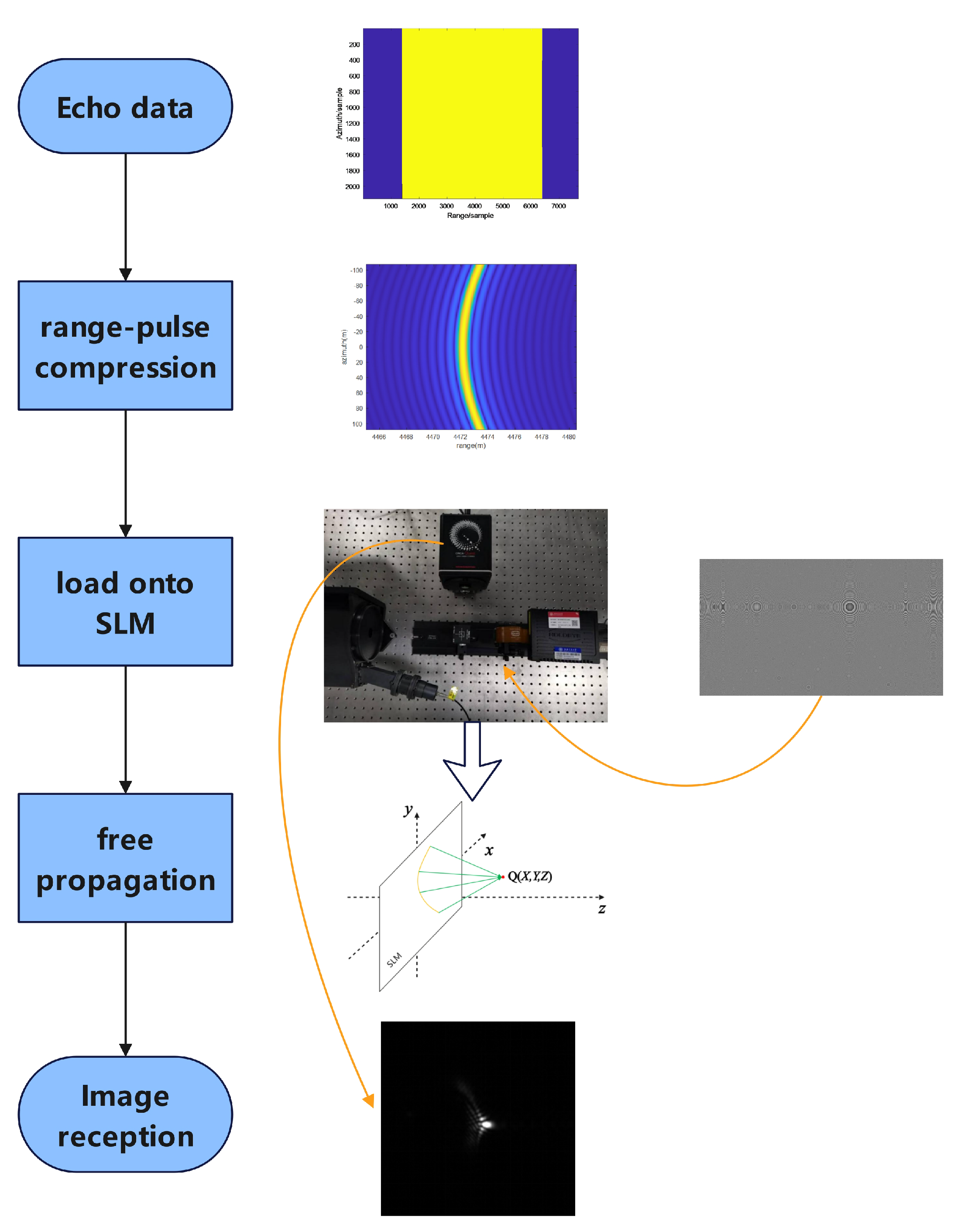
According to the analysis presented in Section 2.2, each individual target point is associated with a focusing ellipse. Efficiently capturing images of multiple-point targets simultaneously hinges on selecting a focal point on each respective ellipse, followed by choosing a connecting surface that intersects these identified points. While aiming for a surface shape that maintains simplicity, the ideal situation involves identifying a planar surface. To simplify the problem, our analysis focuses on cases where the point targets shared the same velocities.

The abscissa of the focal point was specified as $X_{\mathrm{fo}}=2(R_0-R)f_s\Delta /c=k_1(R_0-R)$. The focal point coordinates were set as $(X_{\mathrm{fo}},Y,Z_{\mathrm{fo}})$, according to Equation (20),

$$\begin{array}{c}{Z}_{\mathrm{fo}}=\sqrt{\frac{D}{k_3}[1-\frac{{[k_1(R_0-R)-M]}^2(k_4-k_1^2){(v_y^2+v_1^2)}^2}{D{R}_0^2}]}\hfill \\ =\sqrt{\frac{k_2^4{R}_0^2}{k_4{(v_y^2+v_1^2)}^2}-\frac{k_2^2{(x_0{v}_1-y_0{v}_y)}^2}{{(v_y^2+v_1^2)}^2}}.\hfill \end{array}$$

(27)

Let $x_0=0$ (in cases where $x_0\ne 0$, an alternate reference time can be chosen to ensure $x_0=0$ at $t=0$), then ${R_0}^2={y_0}^2+H^2$. Substituting $R_0=X_{\mathrm{fo}}/k_1+R$ and $y_0^2={(X_{\mathrm{fo}}/k_1+R)}^2-H^2$ into Equation (27) yields the relationship between $X_{\mathrm{fo}}$ and $Z_{\mathrm{fo}}$:

$${Z_{\mathrm{fo}}}^2-\frac{k_2^4-k_2^2{k}_4{v}_y^2}{k_1^2{k}_4{(v_y^2+v_1^2)}^2}{(X_{\mathrm{fo}}+k_{1}R)}^2=\frac{k_2^2{v}_y^2{H}^2}{{(v_y^2+v_1^2)}^2}.$$

(28)

Equation (28) presents a hyperbolic expression within a two-dimensional plane. Using MATLAB (https://www.mathworks.com/products/matlab.html), a graph of $Z_{\mathrm{fo}}$ with respect to $X_{\mathrm{fo}}$ was generated (refer to

Table 1. Parameter List.

Parameter	Value
Speed of light (c)	3 × 108 m/s
Pixel size of SLM ($\Delta$)	3.74 × 10−6 m
Wavelength of laser ($\lambda$)	5.32 × 10−7 m
Wavelength of electromagnetic wave (${\lambda }_0$)	$0.03\mathrm{m}$
Radar sampling rate ($f_s$)	1 × 109 Hz
Radar pulse interval ($\mathrm{PRI}$)	$0.001\mathrm{s}$
The slant distance subtracted (R)	$4800\mathrm{m}$
Radar operating altitude (H)	$4000\mathrm{m}$
Radar velocity ($V_a$)	$100\mathrm{m}/\mathrm{s}$
Bandwidth in range direction ($B_r$)	6 × 108 Hz
Synthetic aperture length ($L_S$)	$216\mathrm{m}$
Target location (P)	$(20,2600,0)$
Target’s velocity along the x-axis ($v_x$)	$10\mathrm{m}/\mathrm{s}$
Target’s velocity along the y-axis ($v_y$)	$1\mathrm{m}/\mathrm{s}$

for relevant parameters). Figure 4 illustrates that the graph closely resembles a straight line. Through linear fitting, the slope and intercept of this line were determined as 1.952410691902430 and 0.233678882644849, respectively. The associated root-mean-square error was calculated to be 5.076 × 10⁻¹⁰.

This led us to consider the possibility of approximating the hyperbola as a straight line. The Taylor expansion of Equation (28) at $X_{\mathrm{fo}}=0$ gives the following expression:

$$\begin{array}{c}{Z}_{\mathrm{fo}}\approx Z_{\mathrm{fo}}\left(0\right)+Z_{\mathrm{fo}}^{\prime }\left(0\right)X_{\mathrm{fo}}\hfill \\ =\frac{\frac{(k_2^4-k_2^2{k}_4{v}_y^2)R}{k_1{k}_4(v_y^2+v_1^2)}}{\sqrt{\frac{(k_2^4-k_2^2{k}_4{v}_y^2)R^2}{k_4}+k_2^2{v}_y^2{H}^2}}{X}_{\mathrm{fo}}+\sqrt{\frac{(k_2^4-k_2^2{k}_4{v}_y^2)R^2}{k_4{(v_y^2+v_1^2)}^2}+\frac{k_2^2{v}_y^2{H}^2}{{(v_y^2+v_1^2)}^2}}.\hfill \end{array}$$

(29)

The resulting slope and intercept were calculated as 1.952408840666066 and 0.233678883785827, respectively. The difference between these computed values and the values obtained from the previous fitting remains below ${10}^{-5}$. Therefore, this approximation was considered reliable.

2.4. Method Summary

After range-pulse compression, the data can be loaded onto the SLM and subjected to imaging through the principle of the free propagation of light. When specific parameters meet designated conditions, the resulting image of an individual moving point target becomes focused onto an ellipse that is oriented perpendicular to the y-axis. The mathematical expressions are shown in Equations (17) and (20). Consequently, any point along this ellipse can be deliberately chosen to receive and reconstruct the image. The simultaneous reception of images for multiple-point targets with identical speeds can be achieved through the strategic positioning of an inclined plane, as demonstrated in Equation (29). To sum up, the entire imaging process is shown in Figure 5.

3. Experiments and Results

In the previous section, we detail the principles and processing flow of the optical imaging method we proposed. In this section, we examine the method from an experimental perspective. Initially, the method’s efficacy is confirmed via straightforward simulation experiments. Subsequently, tailored experiments are orchestrated for distinct scenarios: a single moving point target, multiple moving point targets, and an area target. Ultimately, we investigate the imaging outcomes when moving and stationary targets coexist.

3.1. Experiment 1: Validation of Methodology

To validate the efficacy of the methodology proposed in Section 2, MATLAB simulations were executed. The initial simulation involved an echo generated by a single moving point. Subsequently, a range-pulse compression was performed. Finally, the free propagation of light was simulated using a computational method (Fourier transform was used to calculate Fresnel diffraction, see Appendix B for details), and the resulting light intensity distribution at the plane $z=Z_{\mathrm{focus}}$ (the value of $Z_{\mathrm{focus}}$ was calculated using Equation (26)) is shown in Figure 6. A subset of simulation parameters has been detailed in Table 1. The moving point target was located at $(20,2600,0)$ while maintaining velocities of $v_x=10\mathrm{m}/\mathrm{s}$ and $v_y=1\mathrm{m}/\mathrm{s}$.

As shown in Figure 6, after free propagation, the data demonstrate effective focusing in the azimuth direction; however, the originally well-focused range direction experiences defocusing. This issue can be readily resolved by superimposing a cylindrical lens along the range direction. The effect of introducing the lens is shown in Figure 7, highlighting the sharp focus for the point target. Therefore, the efficacy of the proposed method is affirmed.

3.2. Experiment 2: Single-Point Target Focusing

This experiment aims to use an actual optical setup to focus a single-point target. Both a schematic and a photograph of the optical setup are shown in Figure 8. A 532 nm laser was utilized for the experiment. The SLM used is a reflective liquid-crystal-on-silicon modulator from the HOLOEYE brand, with a pixel pitch of 3.74 μm. Owing to the reflective nature of the SLM, the incorporation of a non-polarizing beam splitter (NPBS) is necessary to change the direction of light propagation. The optical path from the camera to the SLM is denoted as $Z_{\mathrm{focus}}$.

For this experiment, we used the echo data after range compression, which corresponds to the data employed in Experiment 1. In this study, we used an SLM to simultaneously achieve the effects of a cylindrical lens. This was achieved by conducting a Fourier transform on the data intended for loading, followed by multiplication with a matrix equivalent to the lens. The data loaded onto the SLM is shown in Figure A1 in Appendix C. The final imaging results are shown in Figure 9a. The results obtained using the electronic imaging method (employing a matched filter algorithm) are shown in Figure 9b. As shown in Figure 9, the electronic method exhibits a suboptimal focusing effect in the azimuth direction, possibly attributed to the exclusion of target motion effects. In contrast, the method proposed in this paper demonstrates significantly superior focusing performance when compared to the electronic approach.

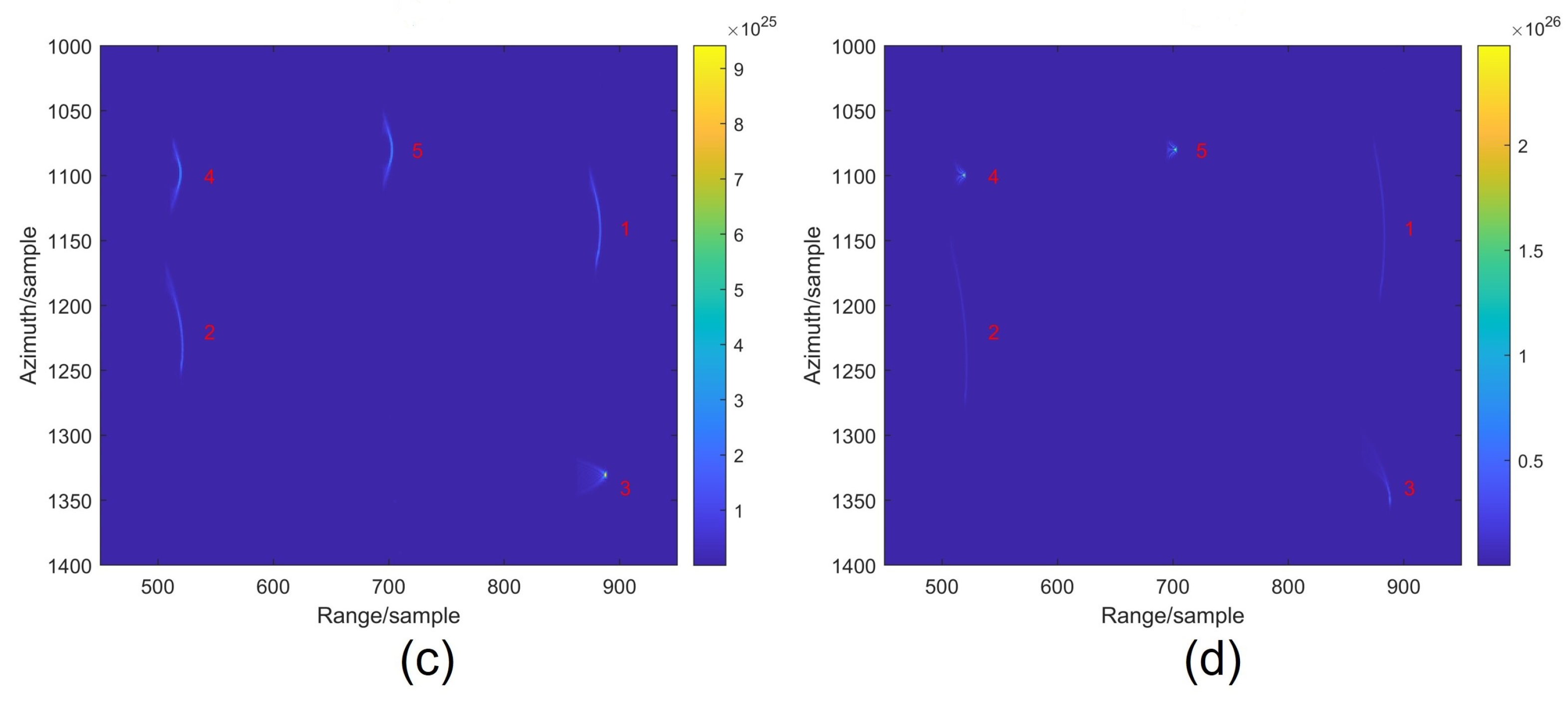
3.3. Experiment 3: Multiple Moving Point Target Focusing

An echo simulation involving three moving points was performed, with simulation parameters listed in Table 1. The velocities assigned to the point targets were $v_x=10\mathrm{m}/\mathrm{s}$ and $v_y=1\mathrm{m}/\mathrm{s}$. From Equation (29), the inclination angle of the inclined plane was calculated as 62.8790°, and the intercept was determined to be 0.2337. To consider the impact of the camera’s tilted placement on receiving performance, compensation was applied. This compensation transformed the loaded data onto the SLM, effectively transforming the tilted plane into a plane perpendicular to the optical axis. The data finally loaded onto the SLM are shown in Figure A2 in Appendix C. The resulting image, shown in Figure 10a, demonstrates a significantly superior imaging result compared to the electronic imaging result illustrated in Figure 10b.

3.4. Experiment 4: Area Target Focusing

A simulated echo features a rectangular area target, achieved by incorporating multiple closely spaced point targets to simulate the area target. The area target measures 4 m in length and 1.8 m in width and is characterized by velocities, where $v_x=10\mathrm{m}/\mathrm{s}$ and $v_y=1\mathrm{m}/\mathrm{s}$. The data finally loaded onto the SLM is shown in Figure A3 in Appendix C. The method proposed for this study was used for imaging, and the results are shown in Figure 11a. In contrast, Figure 11b presents the imaging results generated through the electronic methodology. The electronic imaging results exhibit a severe tailing phenomenon along the azimuth direction, while the optical imaging method does not have this issue.

3.5. Experiment 5: Focusing with Moving and Static Targets

We simulated the echo data containing both a moving point target and a stationary point target, and the velocity of the moving point target remained $v_x=10\mathrm{m}/\mathrm{s}$ and $v_y=1\mathrm{m}/\mathrm{s}$. The optical imaging result, depicted in Figure 12, demonstrates a clear focus on the moving target alongside significant defocusing of the stationary target. Notably, the moving target’s intensity surpasses that of the stationary one, with a comparative analysis revealing the moving target’s intensity to be approximately 14 times greater. Such imaging methodology proves efficacious for scenarios prioritizing the identification of moving targets within a static scence, thereby potentially facilitating the detection of motion amidst stationary backgrounds.

When multiple moving point targets with varying speeds exist in the scene, the results are similar to some extent. The specific experimental procedures and results have been provided in Appendix D.

4. Discussion

In order to facilitate the comparison of the effects of the optical method and the electronic method, we calculated the variances of Figure 9, Figure 10 and Figure 11, respectively, as shown in

Table 2. Variance list.

	a (Optical Method)	b (Electronic Method)
Figure 9 (single point)	7.6359 × ${10}^6$	3.7760
Figure 10 (multiple point)	1.3332 × ${10}^6$	8.1526
Figure 11 (area target)	2.2269 × ${10}^6$	4.6767 × ${10}^5$

. The variances were calculated with the formula shown in Equation (30):

$$Var=\frac{1}{MN}\sum _{m=1}^M\sum _{n=1}^N{(I_{m,n}-\mu )}^2.$$

(30)

Each image has $M\ast N$ pixels. $I_{m,n}$ denotes the pixel value (intensity) at column n, row m. $\mu$ is the mean value of the image, which is defined in Equation (31):

$$\mu =\frac{1}{MN}\sum _{m=1}^M\sum _{n=1}^N{I}_{m,n}.$$

(31)

It can be seen that the variance in the images obtained by the optical method is much larger than that of the electronic method, and the larger the variance, the higher the image quality. We also calculated the peak-to-sidelobe ratios (PSLRs) for Figure 9a,b, which are −12.98 dB and −0.23 dB, respectively. In Figure 10a,b, we selected one point target from each to calculate their PSLRs, which are −0.42 dB and −0.22 dB, respectively.

For a solitary moving point target with a known velocity, it is theoretically possible to determine optimal matched filter parameters, thereby attaining comparatively ideal imaging outcomes. To more effectively contrast the imaging capabilities of our proposed method, we calculated the parameters of the matched filter using accurate motion parameters. Then we employed the refined matched filter algorithm on the echo data from Experiment 2, resulting in the imagery shown in Figure 13a, with a variance of 9.2779 × 10⁵.

Comparing Figure 9a and Figure 13a, it is evident that the image obtained by optical method is broadly similar in contour to Figure 13a. Perhaps the result in Figure 13a has slightly better symmetry and is closer to the ideal sinc function. Nevertheless, the imaging result from the optical method is also commendable. From the standpoint of variance, it even exceeds the performance depicted in Figure 13a. Given the inevitable errors in actual optical paths, some degree of imperfection in imaging results is unavoidable. Moreover, the outcome presented in Figure 13a was achieved utilizing precise motion parameters. If these parameters were obtained by estimation, the result might not be as favorable.

Furthermore, we explored the imaging of individual moving point targets through a parameter search approach. Following pulse compression in the range direction, a set of azimuth matched filters with varying quadratic coefficients were evaluated. The image with optimal imaging performance was chosen according to the maximum variance criterion, as depicted in Figure 13b. The associated variance is 7.7238 × 10⁵, lower than that of Figure 9a. The azimuth profiles of the single-point target images obtained by optical method, optimal matched filter and parameter search approach are shown in Figure 14. The corresponding PSLRs are −12.98 dB, −11.33 dB, and −9.87 dB, respectively.

5. Conclusions

Loading SAR data, which contain moving targets, onto the SLM enables the realization of focusing on these moving targets through the free propagation of light. For a single-point target, focal points are distributed along an ellipse, and the resulting focused image can be captured by a plane perpendicular to the optical axis. For multiple-point targets moving at a uniform speed, a focused image becomes attainable by employing a plane tilted at a specific angle relative to the optical axis. This study establishes a correlation between the position and tilt angle of the plane and target speed, resulting in the successful experimental achievement of focusing on moving targets. The results underscore the superior imaging effect of this method compared to electronic imaging methods. Moreover, the optical imaging system utilized in this study comprises only four components: a laser, an NPBS, an SLM, and a camera, making its structure very simple. The imaging process relies on the free propagation of light, providing minimal processing delay that depends only on the length of the optical path. Certainly, no method is without its shortcomings, and the method we proposed is no exception. Due to the involvement of optical path alignment, it is inevitable that there will be alignment errors, which is a ubiquitous drawback of optical imaging methods. Additionally, limited by the resolution of the SLM, we are currently able to process data of only up to 3840*2160 in size at once. This limitation could potentially be overcome by stitching together multiple SLMs. As technology progresses, it is anticipated that SLMs of higher resolution will become available.

In summary, the method proposed in this paper provides an effective solution for SAR imaging of moving targets. The correlation between the focusing position of these moving targets and their velocities makes it applicable not only for detection and separation but also for velocity estimation. Our future endeavors will delve into exploring additional applications for this method.

References

1. Lan, H.; Liu, X.; Li, L.; Li, Q.; Tian, N.; Peng, J. Remote Sensing Precursors Analysis for Giant Landslides. Remote Sens. 2022, 14, 4399. [Google Scholar] [CrossRef]
2. Pham, T.D.; Yokoya, N.; Bui, D.T.; Yoshino, K.; Friess, D.A. Remote Sensing Approaches for Monitoring Mangrove Species, Structure, and Biomass: Opportunities and Challenges. Remote Sens. 2019, 11, 230. [Google Scholar] [CrossRef]
3. Wang, C.; Chang, L.; Wang, X.S.; Zhang, B.; Stein, A. Interferometric Synthetic Aperture Radar Statistical Inference in Deformation Measurement and Geophysical Inversion: A review. IEEE Geosci. Remote Sens. Mag. 2024, 12, 8–35. [Google Scholar] [CrossRef]
4. Bovenga, F. Special Issue “Synthetic Aperture Radar (SAR) Techniques and Applications”. Sensors 2020, 20, 1851. [Google Scholar] [CrossRef] [PubMed]
5. Xie, T.; Ouyang, R.; Perrie, W.; Zhao, L.; Zhang, X. Proof and Application of Discriminating Ocean Oil Spills and Seawater Based on Polarization Ratio Using Quad-Polarization Synthetic Aperture Radar. Remote Sens. 2023, 15, 1855. [Google Scholar] [CrossRef]
6. Amitrano, D.; Di Martino, G.; Guida, R.; Iervolino, P.; Iodice, A.; Papa, M.N.; Riccio, D.; Ruello, G. Earth Environmental Monitoring Using Multi-Temporal Synthetic Aperture Radar: A Critical Review of Selected Applications. Remote Sens. 2021, 13, 604. [Google Scholar] [CrossRef]
7. Asiyabi, R.M.; Ghorbanian, A.; Tameh, S.N.; Amani, M.; Jin, S.; Mohammadzadeh, A. Synthetic Aperture Radar (SAR) for Ocean: A Review. IEEE J. Sel. Top. Appl. Earth Obs. Remote Sens. 2023, 16, 9106–9138. [Google Scholar] [CrossRef]
8. Nunziata, F.; Meng, T.; Buono, A.; Migliaccio, M. Observing sea oil pollution using synthetic aperture radar measurements: From theory to applications. In Proceedings of the OCEANS 2023—Limerick, Limerick, Ireland, 5–8 June 2023; pp. 1–4. [Google Scholar] [CrossRef]
9. Zhang, Z.; Lin, H.; Wang, M.; Liu, X.; Chen, Q.; Wang, C.; Zhang, H. A Review of Satellite Synthetic Aperture Radar Interferometry Applications in Permafrost Regions: Current status, challenges, and trends. IEEE Geosci. Remote Sens. Mag. 2022, 10, 93–114. [Google Scholar] [CrossRef]
10. Cruz, H.; Véstias, M.; Monteiro, J.; Neto, H.; Duarte, R.P. A Review of Synthetic-Aperture Radar Image Formation Algorithms and Implementations: A Computational Perspective. Remote Sens. 2022, 14, 1258. [Google Scholar] [CrossRef]
11. Pi, Y.; Yang, J.; Fu, Y.; Yang, X. Principle of Synthetic Aperture Radar Imaging; University of Electronic Science and Technology of China Press: Chengdu, China, 2007. [Google Scholar]
12. Munson, D.; O’brien, J.; Kenneth Jenkins, W. A Tomographic Formulation of Spotlight-Mode Synthetic Aperture Radar. Proc. IEEE 1983, 71, 917–925. [Google Scholar] [CrossRef]
13. Wu, C.; Liu, K.; Jin, M. Modeling and a Correlation Algorithm for Spaceborne SAR Signals. IEEE Trans. Aerosp. Electron. Syst. 1982, AES-18, 563–575. [Google Scholar] [CrossRef]
14. Raney, R.; Runge, H.; Bamler, R.; Cumming, I.; Wong, F. Precision SAR processing using chirp scaling. IEEE Trans. Geosci. Remote Sens. 1994, 32, 786–799. [Google Scholar] [CrossRef]
15. Mittermayer, J.; Moreira, A.; Loffeld, O. Spotlight SAR data processing using the frequency scaling algorithm. IEEE Trans. Geosci. Remote Sens. 1999, 37, 2198–2214. [Google Scholar] [CrossRef]
16. Raney, R.K. Synthetic Aperture Imaging Radar and Moving Targets. IEEE Trans. Aerosp. Electron. Syst. 1971, AES-7, 499–505. [Google Scholar] [CrossRef]
17. Sheng, W.; Mao, S. An Effective Method for Ground Moving Target Imaging and Location in SAR System. J. Electron. Inf. Technol. 2004, 26, 598–606. [Google Scholar]
18. Freeman, A.; Currie, A. Synthetic aperture radar (SAR) images of moving targets. GEC J. Res. 1987, 5, 106–115. [Google Scholar]
19. Barbarossa, S. Doppler-Rate Filtering For Detecting Moving Targets with Synthetic Aperture Radars. In Proceedings of the Defense, Security, and Sensing, Orlando, FL, USA, 27–28 March 1989. [Google Scholar]
20. Barbarossa, S.; Farina, A. A novel procedure for detecting and focusing moving objects with SAR based on the Wigner-Ville distribution. In Proceedings of the IEEE International Conference on Radar, Arlington, VA, USA, 7–10 May 1990; pp. 44–50. [Google Scholar] [CrossRef]
21. Xia, X.; Wang, G.; Chen, V. Quantitative SNR analysis for ISAR imaging using joint time-frequency analysis-Short time Fourier transform. IEEE Trans. Aerosp. Electron. Syst. 2002, 38, 649–659. [Google Scholar] [CrossRef]
22. Barbarossa, S.; Farina, A. Detection and imaging of moving objects with synthetic aperture radar. Part 2: Joint time-frequency analysis by Wigner-Ville distribution. IEE Proc. F (Radar Signal Process.) 1992, 139, 89–97. [Google Scholar] [CrossRef]
23. Perry, R.; DiPietro, R.; Fante, R. SAR imaging of moving targets. IEEE Trans. Aerosp. Electron. Syst. 1999, 35, 188–200. [Google Scholar] [CrossRef]
24. Zhu, D.; Li, Y.; Zhu, Z. A Keystone Transform Without Interpolation for SAR Ground Moving-Target Imaging. IEEE Geosci. Remote Sens. Lett. 2007, 4, 18–22. [Google Scholar] [CrossRef]
25. Li, G.; Xia, X.G.; Peng, Y.N. Doppler Keystone Transform: An Approach Suitable for Parallel Implementation of SAR Moving Target Imaging. IEEE Geosci. Remote Sens. Lett. 2008, 5, 573–577. [Google Scholar] [CrossRef]
26. Huang, P.; Liao, G.; Yang, Z.; Xia, X.G.; Ma, J.T.; Ma, J. Long-Time Coherent Integration for Weak Maneuvering Target Detection and High-Order Motion Parameter Estimation Based on Keystone Transform. IEEE Trans. Signal Process. 2016, 64, 4013–4026. [Google Scholar] [CrossRef]
27. Zeng, C.; Li, D.; Luo, X.; Song, D.; Liu, H.; Su, J. Ground Maneuvering Targets Imaging for Synthetic Aperture Radar Based on Second-Order Keystone Transform and High-Order Motion Parameter Estimation. IEEE J. Sel. Top. Appl. Earth Obs. Remote Sens. 2019, 12, 4486–4501. [Google Scholar] [CrossRef]
28. Jao, J.K. Theory of synthetic aperture radar imaging of a moving target. IEEE Trans. Geosci. Remote Sens. 2001, 39, 1984–1992. [Google Scholar] [CrossRef]
29. Vu, V.T.; Sjogren, T.K.; Pettersson, M.I.; Gustavsson, A.; Ulander, L.M.H. Detection of Moving Targets by Focusing in UWB SAR—Theory and Experimental Results. IEEE Trans. Geosci. Remote Sens. 2010, 48, 3799–3815. [Google Scholar] [CrossRef]
30. Sjogren, T.K.; Vu, V.T.; Pettersson, M.I.; Gustavsson, A.; Ulander, L.M.H. Moving Target Relative Speed Estimation and Refocusing in Synthetic Aperture Radar Images. IEEE Trans. Aerosp. Electron. Syst. 2012, 48, 2426–2436. [Google Scholar] [CrossRef]
31. Vu, V.T.; Pettersson, M.I.; Sjögren, T.K. Moving Target Focusing in SAR Image With Known Normalized Relative Speed. IEEE Trans. Aerosp. Electron. Syst. 2017, 53, 854–861. [Google Scholar] [CrossRef]
32. Rosen, P.; Hensley, S.; Joughin, I.; Li, F.; Madsen, S.; Rodriguez, E.; Goldstein, R. Synthetic aperture radar interferometry. Proc. IEEE 2000, 88, 333–382. [Google Scholar] [CrossRef]
33. Cutrona, L.; Leith, E.; Porcello, L.; Vivian, W. On the application of coherent optical processing techniques to synthetic-aperture radar. Proc. IEEE 1966, 54, 1026–1032. [Google Scholar] [CrossRef]
34. Tomiyasu, K. Tutorial review of synthetic-aperture radar (SAR) with applications to imaging of the ocean surface. Proc. IEEE 1978, 66, 563–583. [Google Scholar] [CrossRef]
35. Marchese, L.; Bourqui, P.; Turgeon, S.; Harnisch, B.; Suess, M.; Doucet, M.; Turbide, S.; Bergeron, A. Extended capability overview of real-time optronic SAR processing. In Proceedings of the IET International Conference on Radar Systems (Radar 2012), Glasgow, UK, 22–25 October 2012; pp. 1–5. [Google Scholar] [CrossRef]
36. Wang, D.; Zhang, Y.; Yang, C.; Wang, K. Study on processing synthetic aperture radar data based on optical 4f system for fast imaging. Opt. Express 2022, 30, 44408–44419. [Google Scholar] [CrossRef]
37. Yang, C.; Zhang, Y.; Wang, D.; Wang, K. Compact optical real-time imaging system for high-resolution SAR data based on autofocusing. Opt. Commun. 2023, 546, 129751. [Google Scholar] [CrossRef]
38. Goodman, J.W. Introduction to Fourier Optics, 4th ed.; W. H. Freeman and Company: New York, NY, USA, 2017. [Google Scholar]
39. Lv, N. Fourier Optics, 3rd ed.; China Machine Press: Beijing, China, 2016. [Google Scholar]
Figure 1. Amplitude distribution of SAR echo with a point target after range compression.
Remotesensing 16 01170 g001
Figure 2. Geometry model for radar imaging.
Remotesensing 16 01170 g002
Figure 4. Z fo with respect to X fo .
Remotesensing 16 01170 g004
Figure 5. Moving target imaging process: First, SAR echo data undergo range-pulse compression via computer processing. Next, the phase information is extracted and converted into a grayscale image, and this phase information is then loaded onto a laser using an SLM. Following this, the light compensates for the phase during its free propagation. Finally, a camera is positioned appropriately to capture the finely produced image.
Remotesensing 16 01170 g005
Figure 6. Light intensity distribution of a point target after free propagation. (a) Stereogram. (b) Partially enlarged top view.
Remotesensing 16 01170 g006
Figure 7. Light intensity distribution of a point target after free propagation with a cylindrical lens. (a) Stereogram. (b) Partially enlarged top view.
Remotesensing 16 01170 g007
Figure 8. Optical path utilized in the experiments. (a) Schematic. (b) Physical photograph.
Remotesensing 16 01170 g008
Figure 9. Results of focused single-point target. (a) Optical method. (b) Electronic method.
Remotesensing 16 01170 g009
Figure 10. Focusing results for multiple-point targets. (a) Optical method. (b) Electronic method.
Remotesensing 16 01170 g010
Figure 11. Area target focusing results. (a) Optical method. (b) Electronic method.
Remotesensing 16 01170 g011
Figure 12. Focusing effect when moving and static targets coexist.
Remotesensing 16 01170 g012
Figure 13. Imaging results of a single moving point target using other electronic methods. (a) Optimal matched filter algorithm. (b) Parameter search method.
Remotesensing 16 01170 g013
Figure 14. Azimuth profiles of single-point target imaging results.
Remotesensing 16 01170 g014