Technical Note

Arctic Greening Trends: Change Points in Satellite-Derived Normalized Difference Vegetation Indexes and Their Correlation with Climate Variables over the Last Two Decades

Center of Remote Sensing and GIS, Korea Polar Research Institute, Incheon 21990, Republic of Korea
*
Author to whom correspondence should be addressed.
Remote Sens. 2024, 16(7), 1160; https://doi.org/10.3390/rs16071160
Submission received: 16 January 2024 / Revised: 10 March 2024 / Accepted: 21 March 2024 / Published: 27 March 2024

Abstract

:
In this study, we utilized NDVI data from the moderate resolution imaging spectroradiometer (MODIS) alongside climatic variables obtained from a reanalyzed dataset to analyze Arctic greening during the summer months (June–September) of the last two decades. This investigation entailed a detailed analysis of these changes across various temporal scales. The data indicated a continuous trend of Arctic greening, evidenced by a 1.8% per decade increment in the NDVI. Notably, significant change points were identified in June 2012 and September 2013. A comparative assessment of NDVI pre- and post-these inflection points revealed an elongation of the Arctic greening trend. Furthermore, an anomalous increase in NDVI of 2% per decade was observed, suggesting an acceleration in greening. A comprehensive analysis was conducted to decipher the correlation between NDVI, temperature, and energy budget parameters to elucidate the underlying causes of these change points. Although the correlation between these variables was relatively low throughout the summer months, a distinct pattern emerged when these periods were dissected and examined in the context of the identified change points. Preceding the change point, a strong correlation (approximately 0.6) was observed between all variables; however, this correlation significantly diminished after the change point, dropping to less than half. This shift implies an introduction of additional external factors influencing the Arctic greening trend after the change point. Our findings provide foundational data for estimating the tipping point in Arctic terrestrial ecosystems. This is achieved by integrating the observed NDVI change points with their relationship with climatic variables, which are essential in comprehensively understanding the dynamics of Arctic climate change, particularly with alterations in tundra vegetation.

Graphical Abstract

1. Introduction

The Arctic region has experienced rapid climate change in recent decades, most notably a pronounced temperature increase compared to mid-latitude regions, a phenomenon attributed to Arctic amplification [1].
Consequently, various climate change events have occurred in the Arctic region. Vegetation, a key parameter in climate feedback, significantly influences temperature, surface energy budget, and hydrological balance [2,3,4]. Tundra vegetation dynamics profoundly influence permafrost, mitigating thawing in the summer and increasing soil temperature in snow-related winter [5]. Additionally, variations in atmospheric CO2 concentrations drive vegetation changes, which impact climate change, primarily through alterations in albedo, evapotranspiration, and carbon stocks. These changes trigger various feedback mechanisms, for instance, the ice–albedo feedback where increased vegetation and increasing absorption of solar radiation accelerate Arctic warming [6]. Regional climate change is represented by different trends, such as cooling and warming, that significantly change the Arctic vegetation [7,8,9,10,11]. Therefore, a comprehensive understanding of Arctic vegetation is necessary to determine and respond to the large-scale significance of Arctic climate change [12].
Global warming has led to notable shifts in the density and distribution of tundra land cover [13]. The Arctic tundra is undergoing greening [8,14,15,16,17,18,19,20]. These vegetative changes are complicatedly linked to global warming, exerting substantial influence on the Arctic ecosystem. Understanding the trends and patterns associated with greening is crucial for deciphering its ecological implications and the direction of the Arctic climate. Previous satellite-based studies of Arctic vegetation have focused on overall greening trends [8,14,15,18,21,22,23]; however, the analyses of detailed growth characteristics, such as seasonal variations, annual variations, and change points, have been insufficient. Typically, these studies have leveraged various normalized difference vegetation index (NDVI) datasets such as the global inventory modeling and mapping studies (GIMMS) NDVI and the moderate resolution imaging spectroradiometer (MODIS) NDVI, with the latter being particularly advantageous for long-term, multi-scale trend analyses [21]. Different NDVIs, including annual peak NDVI (Max-NDVI) and time-integrated NDVI (TI-NDVI), have been employed to assess vegetation dynamics [8,14,21]. These NDVI datasets offer certain advantages, like enhanced outlier filtration, but also have limitations.
For instance, the variable dating of Max-NDVI complicates the analysis of time-series features at fixed intervals. At the same time, the smoothed values in TI-NDVI pose challenges in discerning temporal anomalies. Although it is possible to analyze smoothed NDVI data after removing outliers, it is difficult to analyze change points, the strength of the NDVIs, or other factors for specific periods without considering the aforementioned feedback of climate change. In summary, while existing literature elucidates the progression of Arctic greening using satellite data, it should better explain the temporal dynamics of specific phenomena, such as large-scale tipping points. Analyzing the change points in long-term time series data can help explain the dynamics of changes in Arctic terrestrial ecosystems, including the acceleration in variability, the cumulative change, and the climate variables that have more impact relative to the change point.
It is imperative to discern the climatic drivers influencing Arctic greening trends. Generally, a strong correlation exists between changes in Arctic vegetation and temperature [23]. Various research has investigated the relationship between tundra vegetation changes and climatic variables, including the summer warmth index (SWI), snow cover, sea ice extent, and snow thickness [2,14,21,24,25]. However, these studies often vary in approach and have regional, seasonal, and methodological differences in vegetation data. Notably, Arctic vegetation has shown a weak correlation with temperature over time [26]. The tipping point of the tundra was explained using the ice–albedo feedback [6,23,27,28]. Beyond temperature, parameters related to the energy budget are intricately linked to Arctic greening. Most studies of these parameters have been grounded on in situ or modeling approaches [13,24,29,30]. While substantial research has focused on temperature and sea ice, there is a growing need to examine the impacts of energy budget variables and indices on a larger scale. This necessitates a comprehensive analysis integrating temperature and energy budget changes with Arctic vegetation dynamics.
This study aimed to investigate the temporal dynamics and driving forces of Arctic greening trends over the past two decades by employing MODIS NDVI data. We utilized monthly NDVI data, which are less affected by the transformation of peak periods and smoothing, to detect the change point in Arctic vegetation trends using Bayesian statistics. Based on this change point, we analyzed how the characteristics of Arctic greening change across various temporal scales. In addition, we analyzed the correlation between Arctic greening and both temperature and energy budget parameters (e.g., net radiation and turbulent heat flux) in the periods before and after the identified change point to determine the climatic factors governing these patterns across different temporal scales.

2. Materials

2.1. NDVI

NDVI is a vegetation index that uses the spectral properties of vegetation to evaluate their approximate health. NDVI is calculated using the reflectance difference between the near-infrared and visible spectra in the following way [31]:
NDVI = (NIRRed)/(Red + NIR)
where NIR is the reflectance in the near-infrared region and Red is the reflectance in the red region. As most plants absorb solar radiation in the photosynthetically active radiation (PAR) spectral region, which ranges from 400 to 700 nm (visible), and reflect/re-emit energy at longer wavelengths (near-infrared), higher NDVI values represent healthier vegetation. NDVI has been widely used in many studies of vegetation dynamics [32,33]. Variations in NDVI data are driven by weather and ecosystem components; therefore, a vegetation condition index was developed to estimate the impact of weather on vegetation [34].
The MODIS NDVI dataset (MOD13C2V006) serviced by the National Aeronautics and Space Administration (NASA) was used for this study; the data covered the period 2000–2020. The data are formatted in the climate modeling grid (GMC) of 0.05-degree pixels that provide monthly averaged observations. According to the MODIS user guide [35], the valid range of the NDVI data is from −0.2 to 1.0; therefore, the pixels outside this range were first masked in our study.

2.2. Climate Parameters

Various variables have been collected to analyze the impact of climatic variables’ impact on changes to tundra vegetation [2,14,21,24,25]. This study focuses specifically on tundra vegetation and the complicated relationships between these variables that directly influence vegetation feedback.
Typically, vegetations thrive at high temperatures and under humid conditions; however, the Arctic region is generally characterized by its cold and dry climate. Due to climate change, the Arctic has become warmer and moister, and previous studies focused predominantly on temperature and atmospheric conditions. The previous studies used the summer warmth index (SWI) to represent temperature conditions [2,14,21,25], while this study used surface air temperature data from the same period as the NDVI data. Additionally, land surface temperature (LST) was used as a factor to analyze the impact of temperature on the ground surface where vegetation was present. Although albedo is often used as an energy budget related to surface conditions, this study examined net radiation, surface sensible heat flux (SSHF), and latent heat flux (SLHF) instead to provide a comprehensive interpretation of the surface radiation and heat budgets. The sign conventions of net radiation directions are as follows: positive for downward (atmosphere to surface) and negative for upward (surface to atmosphere). However, SSHF and SLHF use the opposite directions—positive for upward (surface to atmosphere) and negative for downward (atmosphere to surface).
Five climatic variables (Table 1) were collected and all the data were extracted from satellite observation (MODIS) and climate reanalysis (ERA5) datasets. Snow and ice data were not included as the study was conducted for the summer season.

3. Methods

3.1. Study Area and Period

The focus of this research was the terrestrial Arctic region [39,40], a diverse landscape comprising barren lands, graminoid, prostrate shrub, and erect shrub vegetations, wetlands, and ice, as categorized by the circumpolar Arctic vegetation map (CAVM) [41]. The study area is poleward of the tree line, with low summer temperatures (an average of under 12 °C in July [41]), limited annual precipitation, and a short growing season [5]. The vegetation comprises mosses, lichens, dwarf shrubs, sedges, grasses, and rushes [5,42]. Notably, the vascular plant cover, including graminoid cover, shrubs, and trees, shows an increasing trend [5].
Due to the reliance of NDVI measurements on solar radiation, data acquisition is constrained during polar nights. NDVI data is obtained from the red and NIR bands, the primary source of which is solar radiation. Hence, a preliminary assessment of the spatiotemporal validity of the dataset is critical. This involves analyzing the observation frequency at each pixel location, guided by the quality control annotations for monthly pixel reliability provided in the MOD13C2V006 dataset. For a comprehensive understanding of the quality control methodologies employed, consultation of the MODIS user guide [35] is recommended.
Spatial distribution maps of valid NDVI points (Figure 1) reveal a significant presence of valid observations primarily between June and September. Outside this temporal window, the proportion of valid data points dropped below 20% during the study period. A notable reduction in valid data points was observed at higher latitudes, particularly in the vicinity of the Laptev and Kara Seas in the Russian Arctic regions, where the percentage of valid observations was markedly low. Additionally, a temporal analysis based on the monthly time series of valid data points indicated an increase in missing values, particularly in June of the early 2000s.
Therefore, the research period spanned from June to September, based on the spatial and temporal distribution of valid NDVI observations. Data were utilized in two approaches: Monthly (June–September) and Summer (average of data from June to August).

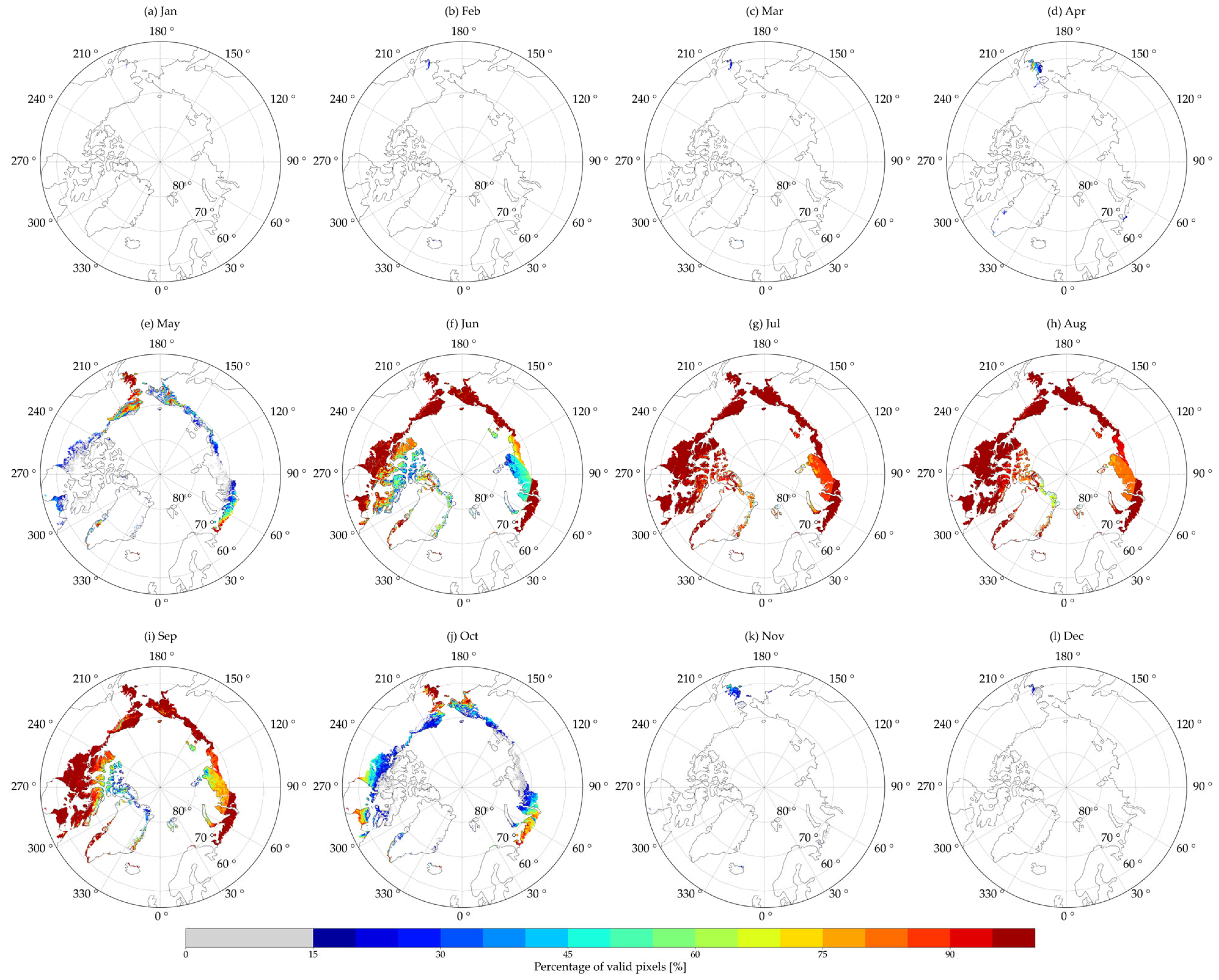
3.2. Characteristics of NDVI Time Series Data

This study aimed to characterize the trends in Arctic NDVI data from the last 20 years and assess the quantitative relationship between NDVI and climate variables. To achieve these objectives, we conducted various statistical evaluations and correlation analyses as follows.
We explored the spatiotemporal dynamics within the study period using multiple statistical methods. Arctic greening and browning can be described from a remote sensing perspective [26]. Greening refers to an increase in vegetation indices, while browning represents the reverse [18]. Selecting a robust statistical approach is crucial for estimating Arctic greening, given the pronounced seasonality in vegetation changes [15,18,21].
For trend detection, we applied the Mann–Kendall test [43,44] and Sen’s slope estimator [45]. The Mann–Kendall test is a widely recognized method for trend analysis in meteorological and hydrological studies [46,47], with foundational details provided by Mann [43] and Kendall [44]. In the research, the significance level was set at a p-value of 0.05 in the Mann–Kendall test. Although the Mann–Kendall test is commonly used to identify annual trends in various research domains, caution is advised when interpreting these trends, especially when they are nonlinear and exhibit change points. Sen’s method offers a nonparametric approach for estimating trends in time series data [45].
The change points in NDVI data can be used as reference points for land-based changes in the analysis of climate change. To detect change points in NDVI time series data, we employed the Bayesian model averaging time series decomposition algorithm called Bayesian Estimator of Abrupt change, Seasonality, and Trend (BEAST) [48]. BEAST is a widely used method in various fields, including phenology, vegetation changes, and dam displacement [49]. BEAST decomposes the time series into seasonal and trend changes to quantify change probabilities using a Bayesian model. The following equation includes the four decomposed components: trend, seasonal variation, abrupt change (i.e., change points), and noise (i.e., residual).
y t = S θ s + T θ T + ε
where y(t) is the time series (NDVI in this study), S is the seasonality, T is the trend, θ s is the change point of the seasonal signal, θ T is the change point of the trend signal, and ε is the gaussian random error [48]. We used annual NDVI data, which are time series data with seasonality removed, as only one value is used for each year. Therefore, the seasonality-related component can be ignored, simplifying the time series decomposed in this study as follows [48]:
y t = T θ T + ε
In our study, we performed a time series analysis of NDVI data, dissecting them into trends, change points, and residuals. This allowed us to closely examine NDVI trends occurring before and after each identified change point. In the results of change points detected using BEAST, two crucial factors, namely number of change points and ranked by probability of occurrence, are essential for obtaining a more accurate interpretation of the change points detected.
The term number of change points refers to the change points observed in the analyzed time series data and their respective probabilities of occurrence. In this study, the change point occurrence probability was calculated for up to four change points, and subsequently, the case with the highest probability was determined. The mode denotes the number of change points with the highest probable occurrence.
The term ranked by probability of occurrence refers to the list of probable trend change points ranked by probability of occurrence. Therefore, it detects the points where change points can occur and provides information about their probabilities. The rank means priority and the trend change point means the time when a change point occurs. The rank is determined by the probability of change point occurrence. Notably, a change point does not necessarily occur when the detection process is performed. To deem the candidate a true change point, it is essential to verify primarily high probability and to consider the proportion of probabilities among the candidates. The number of ranks is not fixed because rank represents all periods within the significance level of the probability of occurrence.
Anomaly analysis was employed to differentiate between ongoing and accelerated NDVI changes. Generally, anomalies are calculated using differences in climatology. However, we conducted an anomaly analysis to determine whether the greening of the Arctic was accelerated based on the start year, as follows:
Anomaly = Xt − X2000
where Xt is the value of the time series data in the current year and X2000 is the value of the time series data in the starting year, 2000. These anomalies were computed relative to the baseline year in the time series. This method allowed us to assess the degree of change from the start year, with ‘anomaly’ in this context being distinctly defined by the ‘residual’ in the BEAST method.

3.3. Relationship with Climate Variables

In this study, we conducted a correlation analysis to examine the relationship between NDVI and various climatic factors over the study period. Our approach involved using a consistent NDVI dataset while aiming to establish a more comprehensive correlation with temperature and energy budget parameters. Furthermore, we distinguished correlations at both annual and monthly scales, specifically analyzing summer versus month-to-month variations. To match the spatial resolutions of different climatic variables, we employed the great circle distance (GCD) method.
We initiated our analysis using Pearson’s correlation to investigate the relationship between NDVI and five key climatic variables, as detailed in Table 1. This allowed us to compute correlation coefficients for each variable and to discern variations in the intensity of relationships before and after identified change points. Additionally, we analyzed the time series patterns of climatic variables through anomaly, differences between atmospheric and surface temperature, and the Bowen ratio (ratio of sensible heat flux to latent heat flux) to understand heat distribution dynamics.
It is also crucial to consider potential time lags when analyzing vegetation–climate relationships, as reactions may not be immediate. For NDVIs, valid pixels were primarily observed from June to September. To accommodate this, we explored time-lagged correlations by adjusting the periods of climatic variables in one-month steps relative to the fixed NDVI period. For example, we calculated correlation coefficients for the NDVI data from June to September against climatic variables from May to August (Month − 1), from June to September (Month + 0), and from July to October (Month + 1), effectively analyzing NDVI correlation with climatic variables over a span of three months both prior to and following the fixed period.

4. Results

4.1. Characterization of NDVI Time Series Data

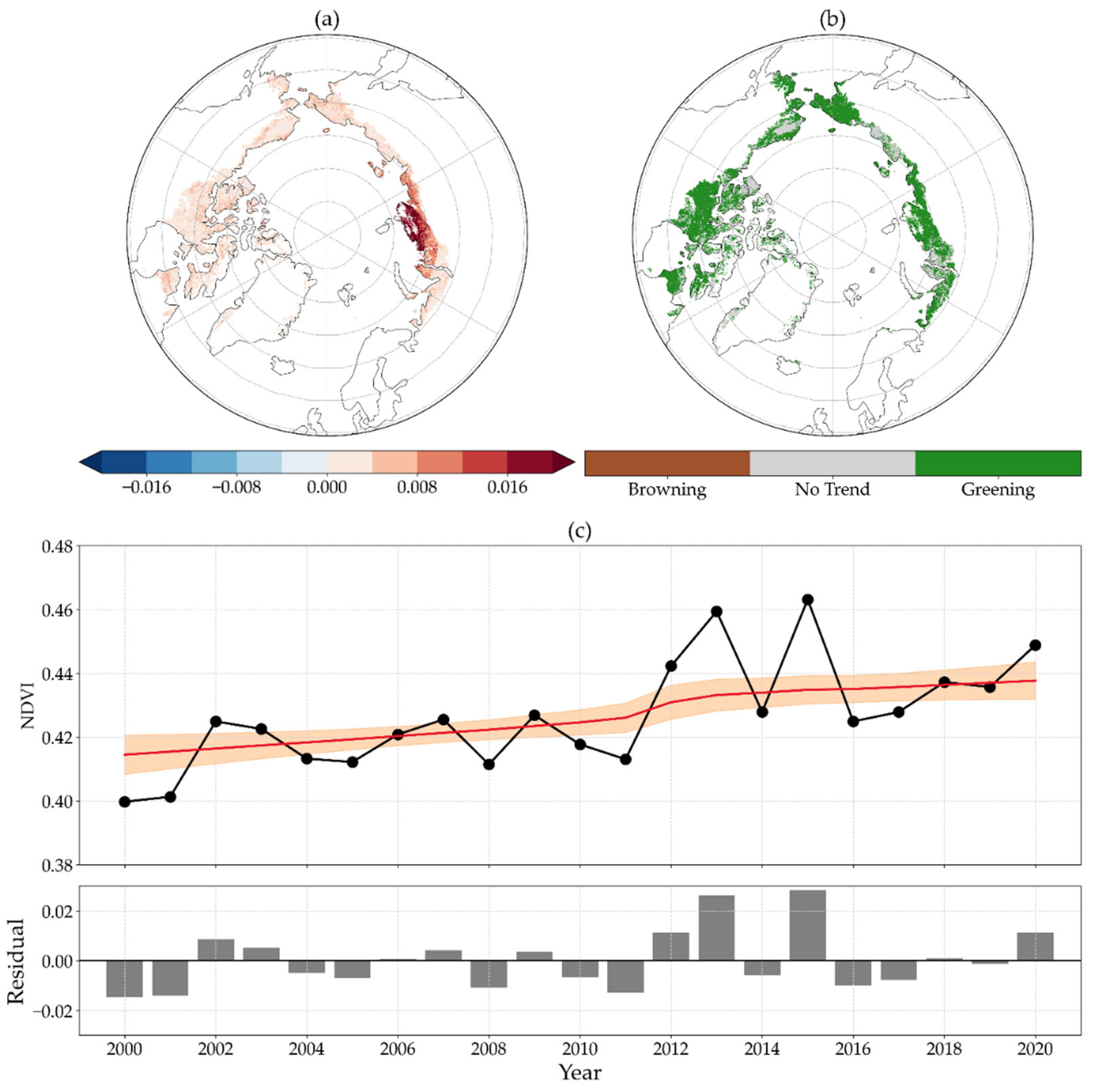
4.1.1. Long-Term Spatiotemporal Trends in NDVI Data

The summer NDVI changes in tundra over the last two decades were estimated to understand large-scale vegetation changes. The annual trend was determined based on the summer NDVI using Sen’s slope, and the Mann–Kendall test was employed to extract the greening area. Figure 2 shows the resulting spatial distributions of the annual trends and the Arctic greening area.
The annual NDVI trends turned out to be positive throughout the tundra, regardless of the region. The spatial distribution of trends in Figure 2a is in line with those reported in previous studies. Annual changes in Max-NDVI and TI-NDVI also showed an increasing trend over the tundra based on MODIS or Landsat products [17,18,21]. Summer NDVI, Max-NDVI, and TI-NDVI commonly indicated significant Arctic greening. Moreover, the greening persisted for two decades from 2000 to 2020. Almost all the tundra areas undergo Arctic greening annually, as shown in Figure 2b. However, some areas are presented in shaded gray (indicating no trend) because they had positive trends but did not meet the significance level.
We conducted another analysis to assess large-scale changes and comprehensively evaluate how the entire Arctic tundra had changed over the given period. The summer NDVI data were spatially averaged across the entire Arctic tundra and the year-to-year changes were estimated, as depicted in Figure 2c. The time series data were decomposed into trends and residuals that describe the temporal evolution of NDVI. The black dotted line, red line, and gray shade represent the summer NDVI data, the trend calculated using BEAST, and the standard deviation of the trend, respectively. The trend indicates an increase of 1.8% per decade at a significant level (p < 0.001). The bar plot in Figure 2c displays the residuals, which are the differences between the NDVI and its trend. The time series residuals indicate that there were dynamic changes in 2013 and 2015; higher NDVIs exceeding 0.02 were observed compared to other periods.

4.1.2. Change Points in Monthly and Summer NDVI Data

The characteristics of the Arctic vegetation time series data were further analyzed using BEAST. Since residuals at a specific point in Figure 2c show a significant increase compared to other periods, it suggests the presence of a singularity during that specific period rather than a typical linear trend. Change point detection in both summer and monthly data was carried out using BEAST; the results are summarized in Table 2. They are divided into ‘number of changepoints’ and ‘ranked by probability of occurrence’ as described in the ‘Method’ section.
First, we had to check the ‘Mode’ of the number of change points. Mode indicates the number of change points in the time series data. For summer (averaged), the mode was zero, indicating that there is likely no change point. In contrast, for June, the mode was one, implying that there is a possibility of one change point during the period. Based on this outcome, it was possible to infer the number of change points in the NDVI data during the particular period.
Second, we focused on ‘Rank’ and ‘Trend Changepoints’ in ranked by probability of occurrence. Rank is a ranking that occurs at a change point in a time series, and Trend Change is the corresponding period. Therefore, Mode and Rank must be considered when detecting change points. In other words, if the mode is 1, the change point is up to the first rank, and if the mode is 2, the change points are up to the second rank.
For the summer, the probability of a change point trend occurring was highest in 2012 (i.e., rank 1); however, the number of change point modes detected was zero, because the difference with the second highest (i.e., rank 2) was not sufficiently large. For that signal, no change point was observed, implying that the imaginary change point in 2012 was not acceptable, considering the trend. In contrast, for June 2012, a trend in change point occurred (i.e., mode 1), with a larger difference in probabilities between rank 1 and rank 2. The 48% probability indicates that there was one change point in 2012.
Overall, the summer NDVI data had a 52.1% probability of having no change points, suggesting that no distinct change point was identified in the summer NDVI data. However, during time series decomposition, the residuals had a dynamic pattern in 2013 and 2016, as shown in Figure 2c. To have a closer look at this, we searched for change points in each of the monthly NDVI data, and two change points were identified in the June NDVI and September NDVI data.
For the June NDVI data, one change point occurred with a 48.2% probability. The highest probability of change point occurrence was in 2012 at 39.7%. Similarly, for the September NDVI data, there was a 67.8% probability of one change point occurring, with the highest probability of 73.6% occurring in 2013. The years 2012 and 2013 were notable periods for changes in sea ice extent. The year 2012 marked a record low in sea ice extent; however, the area recovered quickly and was near average in 2013 [50]. The change points in NDVI occurred in 2012 and 2013. In other words, change points occurred in both land and ocean climate variables simultaneously.

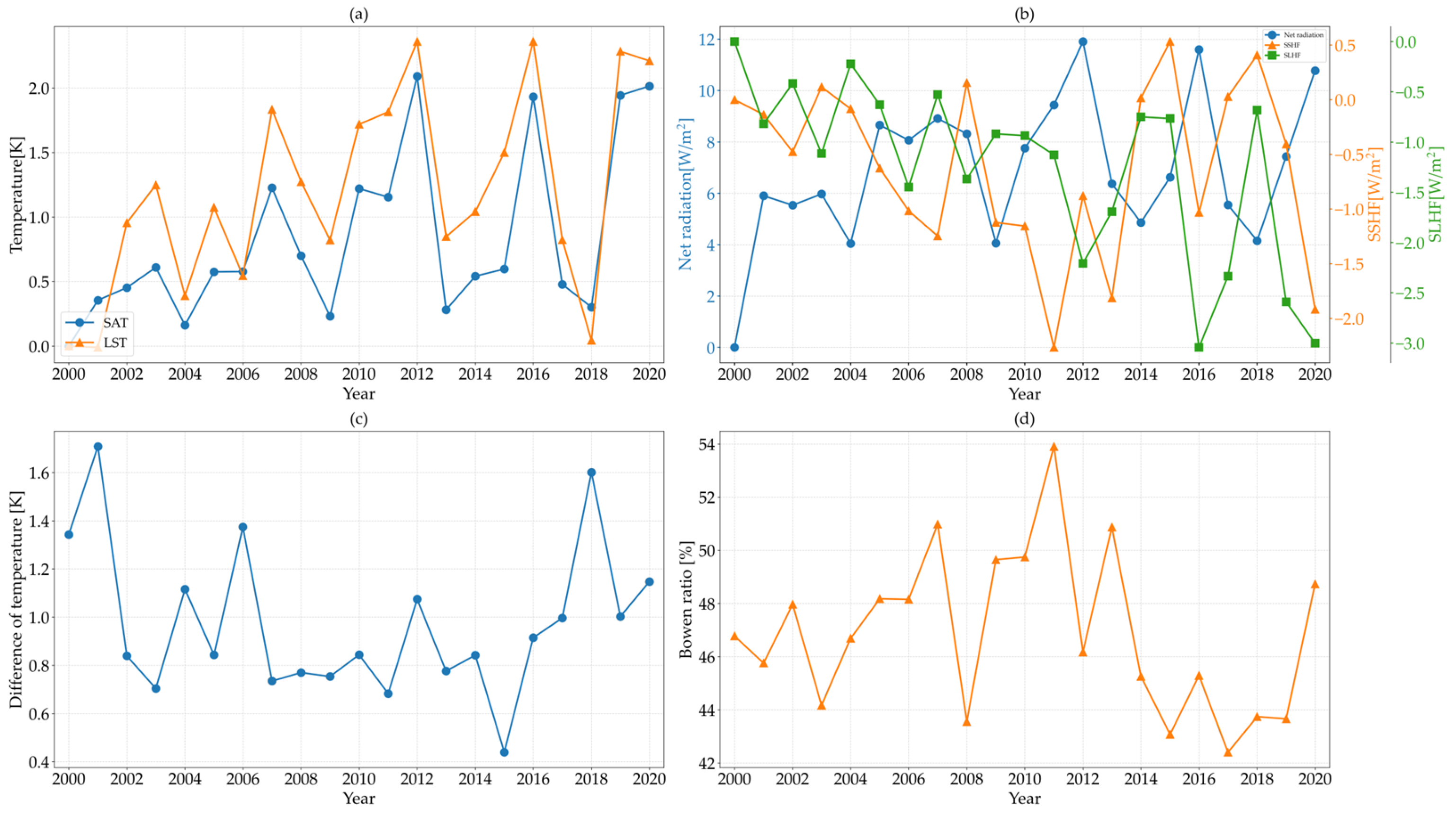
4.1.3. Analysis of NDVI Time Series Data Based on a Temporal Scale

The time series analysis applied to the monthly NDVI data resulted in a more detailed characterization of the dynamic changes observed in the summer NDVI data. Figure 3 displays the monthly NDVI trend, the difference between before and after change point occurrence, and the anomaly in monthly NDVI. In Figure 3a, the trends for July and August NDVI data showed a steady increase with no change points, while the existence of change points in Table 2 was confirmed, showing clearly different trends for June and September NDVIs. The overall upward changes are common to all the monthly NDVIs; however, the jumps between 2012 and 2013 are specific for the June and September NDVIs only.
We estimated the changes in NDVI in seasonal growing cycles over the study period by analyzing how they changed before and after the detected change points. Since the change point in 2012–2013 occurred with high probability, we selected 2012 as the division year. The year-to-year averaged monthly NDVIs for 2000–2012 were termed NDVIPre, and those for 2013–2020 were termed NDVIAft. NDVIAft was higher than NDVIPre for all the summer months, as shown in Figure 3b.
Besides the overall difference between NDVIPre and NDVIAft, larger increases were also observed in June and September. This indicates a strengthened pattern over time in a growing seasonal cycle with the same trend.
The anomaly in the acceleration of Arctic greening was calculated based on the 2000 start year. If the anomaly represents an increase over time and is a positive value, it indicates an acceleration of Arctic greening from the starting year. The anomaly showed a tendency to increase across all the given periods. The anomaly indicates an increasing trend of 0.2% per decade, with a p-value of < 0.001 (p-value < 0.002 in the September NDVI) based on the Mann–Kendall test. In addition, all periods had positive anomalies, except the September NDVI. Although negative anomalies were observed in the September NDVI until 2012, they subsequently turned positive. This is in line with the change point detection results where the September NDVI increased significantly after 2013.

4.2. Relationship between Arctic NDVI and Climate Variables

4.2.1. Relationships between All-Study Period NDVI Data

We analyzed the relationships between vegetation and climatic variables at the same spatial and temporal scales over the past two decades. This analysis assists with explaining changes in Arctic vegetation.
Table 3 represents Pearson’s correlation coefficients between NDVI and the seven climatic variables listed in Table 1. The highest correlation coefficient for each category is indicated in bold. The correlations estimated in this study were slightly weaker than those reported in the previous studies [2,14,21,25] by 0.45–0.7. The decreased correlation over time suggests that, in addition to temperature, other climate variables have become more influential. This was supported by comparing the relative strengths of the correlation coefficients between the seven climatic variables. For example, the surface latent heat flux (SLHF) exhibited a stronger correlation with summer NDVI than temperature, even though it was previously widely recognized that temperature drives vegetation change.

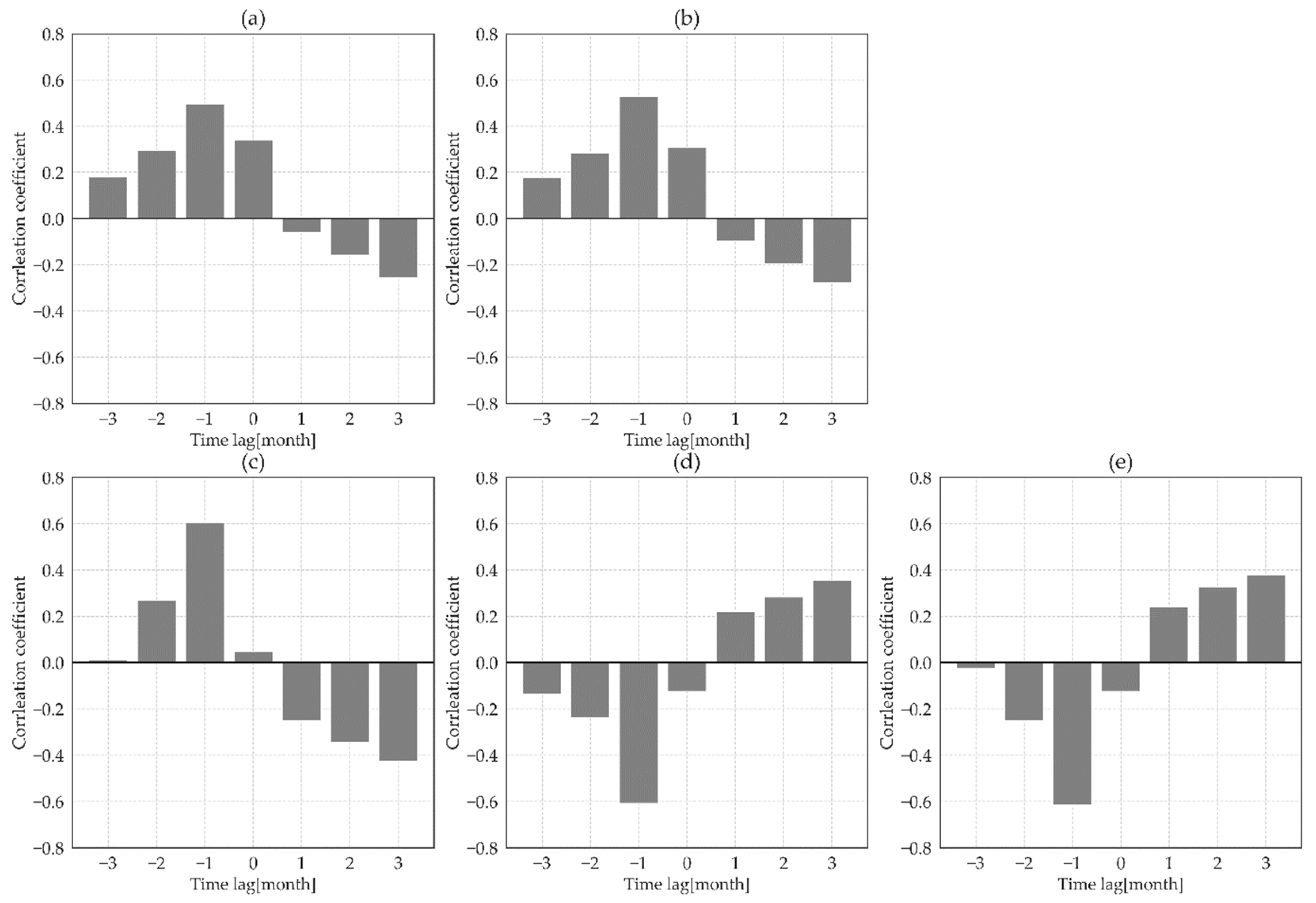
4.2.2. Relationship between Summer NDVIs

We calculated correlation coefficients for the before- and after-periods based on the change point to better analyze the relationship between vegetation changes and climate variables. We compared them with all periods (Table 3 and Table 4). Compared to the correlation coefficients for the summer in Table 3, the correlation is halved when the period after the change point is included. Compared to the previous study [26], the correlation between climate variables and tundra NDVI decreases when more recent periods are included.
The time series patterns of climate variables were analyzed to understand the reasons for the low correlation with NDVI after the change point. For most variables, the interannual differences were amplified around the NDVI change point, resulting in a pattern of high variability (Figure 4a,b). Regarding temperature, both SAT and LST showed a low–high peak change on a 4-year cycle, and the variation increased, with higher amplification after 2012 than before.
The lowest peak in the difference between air and surface temperature occurred in 2015, a period of anomalously high summer NDVI. Around this time, the difference between air and surface temperature decreased and then began to increase again, and the trend of the difference changed from negative to positive (Figure 4c). This means that the mixing between the atmosphere and the surface became more robust, and the blocking of the two boundaries became stronger again around this period.
The energy budget variables showed a pattern similar to that of temperature; anomaly variation increased after 2012. The net radiation showed an increasing trend, and SSHF and SLHF showed decreasing trends. These indicate an increase in the energy absorbed by the surface, suggesting an increase in surface thermal energy. In addition, the Bowen ratio of the time series data was analyzed to determine the heat distribution in the atmosphere. The Bowen ratio pattern peaked in 2011 (Figure 4d). At this time, the Bowen ratio pattern switched from increasing to decreasing. The increase in sensible heat was followed by a decrease in latent heat, indicating that the Arctic has been experiencing an increase in atmospheric evaporation in recent years. The variability in all the variables has increased since 2012; this characteristic reduced the correlation between NDVI and climate variables.

4.2.3. Relationships between Monthly NDVI and Climate Variables

Monthly correlations were analyzed to detect the relationship between climate variables and NDVI during the year. Cross-correlation was calculated to determine the before and after values of the variables (Figure 5). Since the NDVI data are only available from June to September, we analyzed a three-month cross-correlation. As a result, all climate variables (temperature and energy budget) and the vegetation index have a time gap of one month. The results showed that all climate variables exhibited their highest correlations in the previous month, suggesting that the changes in temperature [26] and energy budget variables had a significant impact on NDVI. This finding implies that the change in NDVI, and hence vegetation, could be used as an indicator to understand Arctic climate change better.

5. Discussion

Our study analyzed the spatiotemporal dynamics of tundra vegetation over the last two decades, examining the evolution of satellite-derived NDVI and its correlation with various climatic variables. Consistent with previous research [8,14,18,22], we observed a long-term increasing trend of 1.8% per decade in summer monthly NDVI data, providing strong evidence for Arctic greening. Beyond this, our study utilized a state-of-the-art Bayesian method, BEAST, to provide the characterizations of vegetation changes, including detecting critical change points across the Arctic tundra. The time series residuals indicate that there were dynamic changes in 2013 and 2015; higher NDVIs exceeding 0.02 were observed compared to other periods. We suspect that these periods included the vegetation change points. This large-scale time series singularity could be used as a critical point for detecting changes in the Arctic terrestrial area and analyzing Arctic climate change.
Two significant change points were identified in June and September of 2012 and 2013, similar to the characteristics of sea ice extent [50]. This finding underscores the interconnection between terrestrial and sea ice changes, resonating with the existing literature on the association between reduced sea ice and vegetation dynamics [14]. The change points suggest several possibilities. The NDVI trend strengthened and the range of values generally increased compared to the previous period. It is possible to change the composition of the vegetation type (e.g., barren to grass or grass to shrub) in the tundra region. It also suggests a possible lengthening of the growing season, as the change points in the NDVI data were observed in June and September. In other words, the change points are likely periods when various changes in tundra vegetation may have occurred.
Our analysis focused on the June–September period. This is crucial for understanding the changes in the length of the growing season of Arctic vegetation, which typically spans May–September [16]. These months are the periods associated with the onset and offset of growth, respectively. These two factors are essential when analyzing the length of the vegetation growth season. An extended growing season not only indicates a longer thaw period for the tundra but also impacts permafrost dynamics. Our study specifically investigated NDVI variations before and after the change point, uncovering notable differences, particularly in the June and September NDVI data for the critical growing season. An anomaly analysis revealed that Arctic greening is not merely continuing but accelerating at a rate of 2% per decade. Therefore, it simultaneously exhibits a change point. Overall, our results indicate accelerated Arctic greening over time. This is supported by the increasing annual and anomalous trends in the tundra NDVI.
All variables were highly correlated in the period before the change point, similar to the results of previous studies [2,14,21,25]. It has also been reported that the correlation between vegetation and temperature has decreased in recent years [26]. Our results indicate similar levels of correlations when compared with recent temperature correlations (1982–2019), implying the other correlation values may reflect the same changing conditions adequately. This explains why the correlations for the entire summer period were lower than in previous studies and suggests that there are external factors other than temperature and energy variables after the change point. Additionally, the summer Arctic Bowen ratio entered an unstable phase after 2012, contributing to the observed decline in the correlation between vegetation and climate variables (energy and temperature).
The analysis of time-lagged correlations revealed that all key climate variables exhibit their highest correlations with NDVI in the preceding month. This suggests that climatic variables influence vegetation, with NDVI responding accordingly. Therefore, surface atmosphere energy changes appear to significantly impact vegetation changes, highlighting this relationship as a critical parameter for unraveling the mechanisms driving Arctic vegetation dynamics.

6. Conclusions

This study specifically focused on tundra vegetation, aiming to elucidate its relationship with various climatic variables. Notably, a marked acceleration in Arctic greening was observed around 2012–2013, which can be identified as a potential tipping point. During this period, the correlation between vegetation, temperature, and energy diminished by half. This trend implies that factors beyond direct terrestrial influences are likely playing a significant role in driving tundra vegetation dynamics. Additionally, this timeframe coincides with heightened variability in vegetation and climate factors, suggesting a critical juncture for regional changes in the Arctic tundra. Although it is challenging to estimate the exact growing season length from monthly averaged data, our results indicate that the NDVIs of months including the start and end points increased more than in the other periods, implying an indirect possibility of a faster onset and later offset of growth. It was confirmed that the tundra vegetation is becoming greener, and the growing season is increasing.
However, this study’s reliance on observational data (satellite-derived NDVI) and reanalysis data (climatic variables) introduces complexities in establishing a direct causal link between climatic factors and vegetation changes. While our analysis presents an intuitive relationship between these variables, further research incorporating climate modeling is essential for unraveling the underlying mechanisms. A comprehensive understanding of the forces driving vegetation changes necessitates an analysis that extends beyond terrestrial variables to include a broader energy budget, which has emerged as a critical factor in vegetation dynamics. Additionally, examining the horizontal energy transfer between land and ocean and the vertical energy dynamics within the atmosphere, ocean, and sea ice is pivotal to fully comprehending these complex climate feedback processes.

Author Contributions

Conceptualization, M.S. and H.-C.K.; Data curation, M.S.; Formal analysis, M.S. and H.-C.K.; Funding acquisition, H.-C.K.; Investigation, M.S.; Methodology, M.S. and H.-C.K.; Project administration, H.-C.K.; Software, M.S.; Validation, M.S.; Visualization, M.S.; Writing—original draft, M.S.; Writing—review and editing, M.S. and H.-C.K. All authors have read and agreed to the published version of the manuscript.

Funding

This work was supported by Korea Polar Research Institute (KOPRI) grant funded by the Ministry of Oceans and Fisheries (KOPRI PE24040).

Data Availability Statement

The MODIS (https://earthdata.nasa.gov, accessed on 20 March 2024) and ERA5 (https://cds.climate.copernicus.eu/, accessed on 20 March 2024) data used in this study are freely available from NASA and ECMWF.

Acknowledgments

We would like to express our gratitude to the anonymous reviewers for their valuable comments on this study.

Conflicts of Interest

The authors declare no conflicts of interest.

References

  1. Serreze, M.C.; Barry, R.G. Processes and Impacts of Arctic Amplification: A Research Synthesis. Glob. Planet. Chang. 2011, 77, 85–96. [Google Scholar] [CrossRef]
  2. Blok, D.; Schaepman-Strub, G.; Bartholomeus, H.; Heijmans, M.M.P.D.; Maximov, T.C.; Berendse, F. The Response of Arctic Vegetation to the Summer Climate: Relation between Shrub Cover, NDVI, Surface Albedo and Temperature. Environ. Res. Lett. 2011, 6, 035502. [Google Scholar] [CrossRef]
  3. Lawrence, D.M.; Swenson, S.C. Permafrost Response to Increasing Arctic Shrub Abundance Depends on the Relative Influence of Shrubs on Local Soil Cooling versus Large-Scale Climate Warming. Environ. Res. Lett. 2011, 6, 045504. [Google Scholar] [CrossRef]
  4. Bonfils, C.J.W.; Phillips, T.J.; Lawrence, D.M.; Cameron-Smith, P.; Riley, W.J.; Subin, Z.M. On the Influence of Shrub Height and Expansion on Northern High Latitude Climate. Environ. Res. Lett. 2012, 7, 015503. [Google Scholar] [CrossRef]
  5. Heijmans, M.M.P.D.; Magnússon, R.Í.; Lara, M.J.; Frost, G.V.; Myers-Smith, I.H.; Van Huissteden, J.; Jorgenson, M.T.; Fedorov, A.N.; Epstein, H.E.; Lawrence, D.M.; et al. Tundra Vegetation Change and Impacts on Permafrost. Nat. Rev. Earth Environ. 2022, 3, 68–84. [Google Scholar] [CrossRef]
  6. Foley, J.A. Tipping Points in the Tundra. Science 2005, 310, 627–628. [Google Scholar] [CrossRef]
  7. Comiso, J.C. Arctic Warming Signals from Satellite Observations. WEA 2006, 61, 70–76. [Google Scholar] [CrossRef]
  8. Jia, G.J.; Epstein, H.E.; Walker, D.A. Greening of Arctic Alaska, 1981–2001. Geophys. Res. Lett. 2003, 30, 2067. [Google Scholar] [CrossRef]
  9. Hassol, S.; Assessment, A.C.I. Impacts of a Warming Arctic—Arctic Climate Impact Assessment; Cambridge University Press: Cambridge, UK, 2004; ISBN 978-0-521-61778-9. [Google Scholar]
  10. Stow, D.A.; Hope, A.; McGuire, D.; Verbyla, D.; Gamon, J.; Huemmrich, F.; Houston, S.; Racine, C.; Sturm, M.; Tape, K.; et al. Remote Sensing of Vegetation and Land-Cover Change in Arctic Tundra Ecosystems. Remote Sens. Environ. 2004, 89, 281–308. [Google Scholar] [CrossRef]
  11. Goetz, S.J.; Bunn, A.G.; Fiske, G.J.; Houghton, R.A. Satellite-Observed Photosynthetic Trends across Boreal North America Associated with Climate and Fire Disturbance. Proc. Natl. Acad. Sci. USA 2005, 102, 13521–13525. [Google Scholar] [CrossRef]
  12. Raynolds, M.K.; Walker, D.A.; Maier, H.A. NDVI Patterns and Phytomass Distribution in the Circumpolar Arctic. Remote Sens. Environ. 2006, 102, 271–281. [Google Scholar] [CrossRef]
  13. Pearson, R.G.; Phillips, S.J.; Loranty, M.M.; Beck, P.S.A.; Damoulas, T.; Knight, S.J.; Goetz, S.J. Shifts in Arctic Vegetation and Associated Feedbacks under Climate Change. Nat. Clim. Chang. 2013, 3, 673–677. [Google Scholar] [CrossRef]
  14. Bhatt, U.S.; Walker, D.A.; Raynolds, M.K.; Comiso, J.C.; Epstein, H.E.; Jia, G.; Gens, R.; Pinzon, J.E.; Tucker, C.J.; Tweedie, C.E.; et al. Circumpolar Arctic Tundra Vegetation Change Is Linked to Sea Ice Decline. Earth Interact. 2010, 14, 1–20. [Google Scholar] [CrossRef]
  15. Bhatt, U.S.; Walker, D.A.; Raynolds, M.K.; Bieniek, P.A.; Epstein, H.E.; Comiso, J.C.; Pinzon, J.E.; Tucker, C.J.; Steele, M.; Ermold, W.; et al. Changing Seasonality of Panarctic Tundra Vegetation in Relationship to Climatic Variables. Environ. Res. Lett. 2017, 12, 055003. [Google Scholar] [CrossRef]
  16. Arndt, K.A.; Santos, M.J.; Ustin, S.; Davidson, S.J.; Stow, D.; Oechel, W.C.; Tran, T.T.P.; Graybill, B.; Zona, D. Arctic Greening Associated with Lengthening Growing Seasons in Northern Alaska. Environ. Res. Lett. 2019, 14, 125018. [Google Scholar] [CrossRef]
  17. Bhatt, U.; Walker, D.; Raynolds, M.; Bieniek, P.; Epstein, H.; Comiso, J.; Pinzon, J.; Tucker, C.; Polyakov, I. Recent Declines in Warming and Vegetation Greening Trends over Pan-Arctic Tundra. Remote Sens. 2013, 5, 4229–4254. [Google Scholar] [CrossRef]
  18. Myers-Smith, I.H.; Kerby, J.T.; Phoenix, G.K.; Bjerke, J.W.; Epstein, H.E.; Assmann, J.J.; John, C.; Andreu-Hayles, L.; Angers-Blondin, S.; Beck, P.S.A.; et al. Complexity Revealed in the Greening of the Arctic. Nat. Clim. Chang. 2020, 10, 106–117. [Google Scholar] [CrossRef]
  19. Frost, G.V.; Bhatt, U.S.; Macander, M.J.; Epstein, H.E.; Raynolds, M.K.; Waigl, C.F.; Walker, D.A. Eyes of the World on a Warmer, Less Frozen, and Greener Arctic. Glob. Chang. Biol. 2023, 29, 4453–4455. [Google Scholar] [CrossRef] [PubMed]
  20. Ji, L.; Fan, K. Regime Shift of the Interannual Linkage between NDVI in the Arctic Vegetation Biome and Arctic Sea Ice Concentration. Atmos. Res. 2024, 299, 107184. [Google Scholar] [CrossRef]
  21. Frost, G.V.; Bhatt, U.S.; Macander, M.J.; Hendricks, A.S.; Jorgenson, M.T. Is Alaska’s Yukon–Kuskokwim Delta Greening or Browning? Resolving Mixed Signals of Tundra Vegetation Dynamics and Drivers in the Maritime Arctic. Earth Interact. 2021, 25, 76–93. [Google Scholar] [CrossRef]
  22. Bhatt, U.S.; Walker, D.A.; Walsh, J.E.; Carmack, E.C.; Frey, K.E.; Meier, W.N.; Moore, S.E.; Parmentier, F.-J.W.; Post, E.; Romanovsky, V.E.; et al. Implications of Arctic Sea Ice Decline for the Earth System. Annu. Rev. Environ. Resour. 2014, 39, 57–89. [Google Scholar] [CrossRef]
  23. Box, J.E.; Colgan, W.T.; Christensen, T.R.; Schmidt, N.M.; Lund, M.; Parmentier, F.-J.W.; Brown, R.; Bhatt, U.S.; Euskirchen, E.S.; Romanovsky, V.E.; et al. Key Indicators of Arctic Climate Change: 1971–2017. Environ. Res. Lett. 2019, 14, 045010. [Google Scholar] [CrossRef]
  24. Schaefer, J.A.; Messier, F. Scale-Dependent Correlations of Arctic Vegetation and Snow Cover. Arct. Alp. Res. 1995, 27, 38. [Google Scholar] [CrossRef]
  25. Reichle, L.M.; Epstein, H.E.; Bhatt, U.S.; Raynolds, M.K.; Walker, D.A. Spatial Heterogeneity of the Temporal Dynamics of Arctic Tundra Vegetation. Geophys. Res. Lett. 2018, 45, 9206–9215. [Google Scholar] [CrossRef]
  26. Bhatt, U.S.; Walker, D.A.; Raynolds, M.K.; Walsh, J.E.; Bieniek, P.A.; Cai, L.; Comiso, J.C.; Epstein, H.E.; Frost, G.V.; Gersten, R.; et al. Climate Drivers of Arctic Tundra Variability and Change Using an Indicators Framework. Environ. Res. Lett. 2021, 16, 055019. [Google Scholar] [CrossRef]
  27. Chapin, F.S.; Sturm, M.; Serreze, M.C.; McFadden, J.P.; Key, J.R.; Lloyd, A.H.; McGuire, A.D.; Rupp, T.S.; Lynch, A.H.; Schimel, J.P.; et al. Role of Land-Surface Changes in Arctic Summer Warming. Science 2005, 310, 657–660. [Google Scholar] [CrossRef]
  28. Lund, M. Uncovering the Unknown—Climate Interactions in a Changing Arctic Tundra. Environ. Res. Lett. 2018, 13, 061001. [Google Scholar] [CrossRef]
  29. Cho, M.-H.; Yang, A.-R.; Baek, E.-H.; Kang, S.M.; Jeong, S.-J.; Kim, J.Y.; Kim, B.-M. Vegetation-Cloud Feedbacks to Future Vegetation Changes in the Arctic Regions. Clim. Dyn. 2018, 50, 3745–3755. [Google Scholar] [CrossRef]
  30. Juszak, I.; Erb, A.M.; Maximov, T.C.; Schaepman-Strub, G. Arctic Shrub Effects on NDVI, Summer Albedo and Soil Shading. Remote Sens. Environ. 2014, 153, 79–89. [Google Scholar] [CrossRef]
  31. Rouse, J.W.; Haas, R.H.; Deering, D.W.; Schell, J.A.; Harlan, J.C. Monitoring the Vernal Advancement and Retrogradation (Green Wave Effect) of Natural Vegetation. 1974. Available online: https://ntrs.nasa.gov/citations/19750020419 (accessed on 20 March 2024).
  32. Rocha, A.V.; Shaver, G.R. Advantages of a Two Band EVI Calculated from Solar and Photosynthetically Active Radiation Fluxes. Agric. For. Meteorol. 2009, 149, 1560–1563. [Google Scholar] [CrossRef]
  33. Sun, Y.; Knyazikhin, Y.; She, X.; Ni, X.; Chen, C.; Ren, H.; Myneni, R.B. Seasonal and Long-Term Variations in Leaf Area of Congolese Rainforest. Remote Sens. Environ. 2022, 268, 112762. [Google Scholar] [CrossRef]
  34. Zhang, H.; Yin, G.; Zhang, L. Evaluating the Impact of Different Normalization Strategies on the Construction of Drought Condition Indices. Agric. For. Meteorol. 2022, 323, 109045. [Google Scholar] [CrossRef]
  35. Didan, K.; Munoz, A.B.; Huete, A. MODIS Vegetation Index User’s Guide (MOD13 Series); University of Arizona: Vegetation Index and Phenology Lab: Tucson, AZ, USA, 2015; Volume 35. [Google Scholar]
  36. Hersbach, H.; Bell, B.; Berrisford, P.; Hirahara, S.; Horányi, A.; Muñoz-Sabater, J.; Nicolas, J.; Peubey, C.; Radu, R.; Schepers, D.; et al. The ERA5 Global Reanalysis. Q. J. R. Meteorol. Soc. 2020, 146, 1999–2049. [Google Scholar] [CrossRef]
  37. Wan, Z.; Hook, S.; Hulley, G. MOD11C3 MODIS/Terra Land Surface Temperature/Emissivity Monthly L3 Global 0.05 Deg CMG V006. Nasa EOSDIS LP DAAC 2015, 10. [Google Scholar] [CrossRef]
  38. Kato, S.; Rose, F.G.; Rutan, D.A.; Thorsen, T.J.; Loeb, N.G.; Doelling, D.R.; Huang, X.; Smith, W.L.; Su, W.; Ham, S.-H. Surface Irradiances of Edition 4.0 Clouds and the Earth’s Radiant Energy System (CERES) Energy Balanced and Filled (EBAF) Data Product. J. Clim. 2018, 31, 4501–4527. [Google Scholar] [CrossRef]
  39. CAVM Team Team: Circumpolar Arctic Vegetation. Available online: https://cir.nii.ac.jp/crid/1370285708264373123 (accessed on 16 January 2024).
  40. Raynolds, M.K.; Walker, D.A.; Balser, A.; Bay, C.; Campbell, M.; Cherosov, M.M.; Daniëls, F.J.A.; Eidesen, P.B.; Ermokhina, K.A.; Frost, G.V.; et al. A Raster Version of the Circumpolar Arctic Vegetation Map (CAVM). Remote Sens. Environ. 2019, 232, 111297. [Google Scholar] [CrossRef]
  41. Walker, D.A.; Raynolds, M.K.; Daniëls, F.J.A.; Einarsson, E.; Elvebakk, A.; Gould, W.A.; Katenin, A.E.; Kholod, S.S.; Markon, C.J.; Melnikov, E.S.; et al. The Circumpolar Arctic Vegetation Map. J. Veg. Sci. 2005, 16, 267–282. [Google Scholar] [CrossRef]
  42. Mauclet, E.; Hirst, C.; Monhonval, A.; Stevenson, E.I.; Gérard, M.; Villani, M.; Dailly, H.; Schuur, E.A.G.; Opfergelt, S. Tracing Changes in Base Cation Sources for Arctic Tundra Vegetation upon Permafrost Thaw. Geoderma 2023, 429, 116277. [Google Scholar] [CrossRef]
  43. Mann, H.B. Nonparametric Tests Against Trend. Econometrica 1945, 13, 245–259. [Google Scholar] [CrossRef]
  44. Kendall, M.G. Rank Correlation Methods; Griffin: Oxford, UK, 1948. [Google Scholar]
  45. Sen, P.K. Estimates of the Regression Coefficient Based on Kendall’s Tau. J. Am. Stat. Assoc. 1968, 63, 1379–1389. [Google Scholar] [CrossRef]
  46. Gilbert, R.O. Statistical Methods for Environmental Pollution Monitoring; John Wiley & Sons: Hoboken, NJ, USA, 1987; ISBN 978-0-471-28878-7. [Google Scholar]
  47. Sirois, A. A Brief and Biased Overview of Time-Series Analysis of How to Find That Evasive Trend, WMO. In Proceedings of the EMEP Workshop on Advanced Statistical Methods and Their Application to Air Quality Data Sets, Helsinki, Finland, 14–18 September 1998. [Google Scholar]
  48. Zhao, K.; Wulder, M.A.; Hu, T.; Bright, R.; Wu, Q.; Qin, H.; Li, Y.; Toman, E.; Mallick, B.; Zhang, X.; et al. Detecting Change-Point, Trend, and Seasonality in Satellite Time Series Data to Track Abrupt Changes and Nonlinear Dynamics: A Bayesian Ensemble Algorithm. Remote Sens. Environ. 2019, 232, 111181. [Google Scholar] [CrossRef]
  49. Xu, D.; Geng, Q.; Jin, C.; Xu, Z.; Xu, X. Tree Line Identification and Dynamics under Climate Change in Wuyishan National Park Based on Landsat Images. Remote Sens. 2020, 12, 2890. [Google Scholar] [CrossRef]
  50. September|2013|Arctic Sea Ice News and Analysis 2013. Available online: https://nsidc.org/arcticseaicenews/2013/09/ (accessed on 20 March 2024).
Figure 1. Distribution of valid percentages per pixel after applying the quality flag; the gray shading indicates the count of valid pixels below 15% during the study period.
Remotesensing 16 01160 g001
Figure 2. The annual change in NDVI, Arctic greening area, and time series data distribution for the summer periods of 2000–2020: (a) annual NDVI trend, (b) Arctic greening area, and (c) decomposition results of the time series data. The decomposition consists of the trend (red line), the standard deviation of the trend (orange shade), and the residuals (bar plot).
Remotesensing 16 01160 g002
Figure 3. Monthly NDVI time series data collected under various conditions; (a) trends, (b) growing seasonal cycles before/after change points, and (c) anomalies calculated relative to the starting year.
Remotesensing 16 01160 g003
Figure 4. Summer climate variable time series data for the tundra; (a) Temperature anomaly (surface air temperature and land surface temperature), (b) Energy budget anomaly (Net radiation, Surface sensible heat flux, Surface latent heat flux), (c) Difference between surface air temperature and land surface temperature, and (d) Bowen ratio.
Remotesensing 16 01160 g004
Figure 5. Monthly time lag correlations; (a) Surface air temperature, (b) Land surface temperature, (c) Net radiation, (d) Surface sensible heat flux, (e) Surface latent heat flux.
Remotesensing 16 01160 g005
Table 1. Summary of climatic variables used in the study (all data were collected at monthly intervals).
VariablesSpatial ResolutionData SourceReference
Surface Air Temperature (SAT)0.25 degreeERA5 reanalysis product[36]
Land Surface Temperature (LST)0.05 degreeNASA MODIS product[37]
Net Radiation (Rn)1 degreeNASA CERES EBAF product[38]
Surface Latent Heat Flux (SLHF)0.25 degreeERA5 reanalysis product[36]
Surface Sensible Heat Flux (SSHF)0.25 degreeERA5 reanalysis product[36]
Table 2. Summary of change points detected using BEAST.
Number of Change PointsRanked by Probability of Occurrence
ModeProbability (%)RankTrend Change PointsProbability (%)
Summer052.11201232.8
2201610.2
June148.21201239.7
220046.7
July058.51201218.7
220047.7
August047.71201016.0
2200715.3
3201615.2
September167.81201373.6
220044.4
Table 3. Correlation coefficients between vegetation and climate variables in the study periods.
Surface
Air
Temperature
Land Surface TemperatureNet RadiationSurface Sensible Heat FluxSurface Latent Heat Flux
Summer0.290.380.27−0.13−0.42
June0.250.420.27−0.28−0.41
July0.330.34−0.230.240.26
August0.210.260.43−0.02−0.37
September−0.17−0.24−0.420.05−0.06
Table 4. Correlation coefficients between vegetation and climate variables based on the 2012 change point.
Surface
Air Temperature
Land Surface
Temperature
Net RadiationSurface
Sensible
Heat Flux
Surface
Latent
Heat Flux
Before0.650.690.55−0.33−0.59
After−0.23−0.05−0.03−0.220.27
Disclaimer/Publisher’s Note: The statements, opinions and data contained in all publications are solely those of the individual author(s) and contributor(s) and not of MDPI and/or the editor(s). MDPI and/or the editor(s) disclaim responsibility for any injury to people or property resulting from any ideas, methods, instructions or products referred to in the content.

