Abstract
The census and management of hazard-bearing entities, along with the integrity of data quality, form crucial foundations for disaster risk assessment and zoning. By addressing the challenge of feature confusion, prevalent in single remotely sensed image recognition methods, this paper introduces a novel method, Spatially Constrained Deep Learning (SCDL), that combines deep learning with spatial constraint strategies for the extraction of disaster-bearing bodies, focusing on dams as a typical example. The methodology involves the creation of a dam dataset using a database of dams, followed by the training of YOLOv5, Varifocal Net, Faster R-CNN, and Cascade R-CNN models. These models are trained separately, and highly confidential dam location information is extracted through parameter thresholding. Furthermore, three spatial constraint strategies are employed to mitigate the impact of other factors, particularly confusing features, in the background region. To assess the method’s applicability and efficiency, Qinghai Province serves as the experimental area, with dam images from the Google Earth Pro database used as validation samples. The experimental results demonstrate that the recognition accuracy of SCDL reaches 94.73%, effectively addressing interference from background factors. Notably, the proposed method identifies six dams not recorded in the GOODD database, while also detecting six dams in the database that were previously unrecorded. Additionally, four dams misdirected in the database are corrected, contributing to the enhancement and supplementation of the global dam geo-reference database and providing robust support for disaster risk assessment. In conclusion, leveraging open geographic data products, the comprehensive framework presented in this paper, encompassing deep learning target detection technology and spatial constraint strategies, enables more efficient and accurate intelligent retrieval of disaster-bearing bodies, specifically dams. The findings offer valuable insights and inspiration for future advancements in related fields.
1. Introduction
The precision of identifying disaster-prone entities through the natural disaster risk census directly impacts the efficiency and effectiveness of post-disaster relief and recovery endeavors [1]. Consequently, the precise identification of these disaster-prone entities contributes to accurately defining areas at risk of disasters and facilitates continuous monitoring of potential disaster occurrences [2]. However, extracting the targets of disaster-prone entities presents certain challenges. Primarily, the environmental conditions surrounding these entities are often intricate and influenced by geographic features, meteorological conditions, and human activities. Additionally, the diverse characteristics of damage exhibited by disaster-prone entities post-disaster, stemming from variations in structure, morphology, and extent of damage, further complicate the extraction process [3,4]. The combination of these influencing factors gives rise to difficulties in distinguishing between disaster-prone entities and surrounding features, thereby intensifying the complexity of disaster risk delineation.
Currently, data on disaster-bearing entities primarily originate from field surveys and building data [5], demanding substantial human, material, and financial resources [6]. With the advancement of remotely sensed technology, the utilization of remotely sensed target recognition technology has emerged as a crucial method for recognizing and extracting disaster-bearing entities [7,8,9]. Notably, typical disaster-bearing entities, such as dams, bridges, roads, and reservoir embankments, share striking similarities in remotely sensed images. As depicted in Figure 1, they exhibit evident linear and color features, and their relatively concentrated distribution in geospatial space amplifies the challenge of extracting these target disaster-bearing objects, thereby complicating the disaster census. The reliance on feature-based image extraction methods fails to fully exploit structural and textural information in remotely sensed images, leading to diminished classification accuracy at the pixel level. Moreover, an excessive dependence on limited pixel spectral information can constrain the classification results, making it arduous to accurately distinguish between various targets. In essence, feature-based remotely sensed image extraction methods struggle to fulfill the requirements for the high-precision and high-efficiency extraction of disaster-bearing entities.
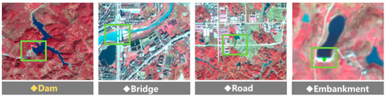
Figure 1.
Features with similar characteristics (The green squares mark the easily confused disaster-bearing bodies).
In recent years, the emergence of deep learning technology has offered innovative solutions to address the constraints of feature-based image extraction methods [10,11]. For instance, Biffi et al. introduced a ground-based RGB image detection method utilizing adaptive training samples to select a deep learning model, effectively overcoming issues of target self-obscuration and mutual occlusion [12]. Similarly, Balaniuk et al. combined cloud computing, free open-source software, and deep learning techniques to automatically identify and classify large-scale mining tailing dams nationwide [13]. With the rapid evolution of this domain, deep learning based on convolutional neural networks (CNNs) has demonstrated robust feature extraction capabilities and high accuracy rates [14]. For example, Shao et al. leveraged nighttime remotely sensed data to enhance ship detection, refining the YOLOv5 algorithm model to effectively improve the accuracy and completeness of ship datasets [15]. Additionally, Yan et al. developed an intelligent, high-precision method for extracting information from tailing ponds, addressing the challenge of incomplete data by enhancing deep learning target detection models. This advancement not only enhances the recognition accuracy of tailing pond failures but also boosts decision-making efficiency in tailing pond management, laying the groundwork for global-scale tailing dam detection [16]. While deep learning stands as a potent machine learning algorithm capable of handling nonlinear and complex data, remotely sensed images remain susceptible to interference from various factors such as background conditions, lighting, and target shape diversity. Deep learning models encounter difficulties in distinguishing targets with high similarity [17,18], as illustrated in Figure 2, where bridges, roads, and reservoir embankments are erroneously categorized under the same label with relatively high confidence levels.
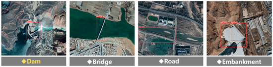
Figure 2.
Deep Learning Misjudged Features (Red boxes represent checkboxes for target tests).
Furthermore, while deep learning models excel at recognizing targets within images, they often lack precise location information about these targets. However, disaster census and post-disaster rescue operations typically necessitate accurate target location data. Consequently, scholars have introduced spatial constraint strategies to enhance the understanding of target shape, structure, and location. For instance, Van Soesbergen et al. devised a globally available remotely sensed imagery method for automated dam reservoir extraction, effectively distinguishing dam reservoirs from natural water bodies to bridge the geolocation data gap between dams and reservoirs [19]. Similarly, Asbury and Aly integrated remotely sensed and Geographic Information System (GIS) techniques to examine the impact of drought on ten selected surface reservoirs in San Angelo and Dallas, Texas, emphasizing the need for continuous monitoring to understand drought effects on reservoirs [20]. Additionally, Yang et al. introduced a GIS-based accident analysis framework centered on spatial feature distribution [21], while Chen et al. proposed a model for assessing human settlement suitability at the village scale, combining decision analysis and spatial analysis for the first time [22]. The spatial constraint strategy delves into the intricate spatial relationships between targets, eliminating various interfering factors that may introduce errors, thus refining the discrimination scope. This approach enables more accurate problem analysis and the development of effective solutions.
In summary, the challenges in recognizing and extracting disaster-bearing objects can be categorized as follows: (1) Distinguishing disaster-bearing objects from surrounding features with similar geometric and spectral characteristics poses a significant obstacle. Consequently, employing a single method for their recognition and extraction proves challenging. (2) The presence of various background factors within the region introduces interference, impacting the accuracy of disaster-bearing body recognition. This interference often leads to confusion between disaster-bearing bodies and other features present in remotely sensed images.
Based on the aforementioned analysis, it is evident that remotely sensed images are vulnerable to interference from background and lighting conditions, as well as the diverse shapes of targets. This poses challenges for deep learning models in distinguishing targets with high similarity during recognition. Consequently, misjudgments can occur, and the precise location of the target remains unknown when using deep learning models alone. However, by integrating spatial constraint strategies, interference factors can be mitigated, and the discriminatory range can be narrowed, aiding the deep learning model in achieving more accurate target localization. Therefore, this paper focuses on dams as a representative example of typical disaster-bearing bodies and explores the feasibility of combining deep learning techniques with spatial constraint strategies. The results demonstrate significant potential for the extraction of typical disaster-bearing bodies using this approach.
The subsequent sections of the paper are structured as follows. Section 2 offers an overview of the study area, detailing the methodological process for dataset construction and the acquisition of additional necessary experimental data. Furthermore, it introduces the concepts and composition of two distinct classes of target recognition models and spatial constraint strategies. Section 3 explores the extraction results achieved through the fusion of deep learning and spatial constraint strategies, along with discussing the evaluation method employed to assess extraction accuracy. Section 4 examines the applicability of the spatial constraint strategy and provides supplementary analysis on target extraction from disaster-bearing bodies in small watersheds. Section 5 summarizes the conclusions drawn from this study.
2. Materials and Methods
2.1. Study Area
As shown in Figure 3, Qinghai Province is located in the hinterland of the Northwest China Plateau, at a longitude of 89°20′–103°05′E and a latitude of 31°40′–39°15′N. The province of Qinghai has the largest number of dams in the world. Its special geographic location and plateau continental climate endow it with a unique hydrological environment, so we take the distribution of dams in Qinghai Province as the research object and dams in various regions around the world as the sample data source [23] and verify the accuracy of the model and algorithms by extracting dams, the typical disaster-bearing bodies in the images of Qinghai Province.
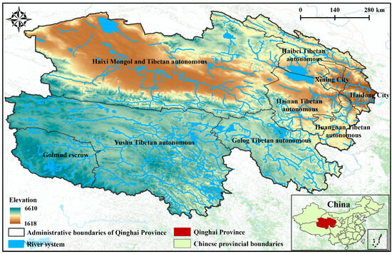
Figure 3.
Study area—Qinghai Province.
2.2. Data
In this study, we utilize Sentinel-2A satellite remotely sensed imagery, ensuring coverage of Qinghai Province with minimal cloud interference (less than 5%). These images boast a spatial resolution of 10 m, as detailed in Table 1 and Appendix B. Leveraging Sentinel-2’s L2A [24] data, which undergoes rigorous radiometric calibration and geometric refinement, enables direct utilization for our analytical purposes. In this paper, we mainly use green and near-infrared bands to extract the water bodies in the study area.

Table 1.
Sentinel II satellite information.
The dataset employed in this study comprises both training and validation sample sets. The quantity and quality of these samples critically influence the classifier’s performance, with an apt selection ensuring accurate feature representation. Thus, a meticulously chosen sample set can effectively mirror real-world conditions and enhance classifier efficacy [25].
Currently, publicly available dam samples primarily consist of conventional digital images captured at close proximity. There exists a notable absence of publicly accessible remotely sensed image datasets, compounded by variations in dam design standards across different countries. As illustrated in Figure 4, (a) depicts the arch-shaped Hoover Dam in the U.S., while (b) showcases the straight-line structure of the Three Gorges Dam in China. Hence, the creation of a comprehensive dam sample dataset becomes imperative [23]. To initiate this process, we establish circular buffers centered on the dam point-type vectors sourced from the Global Reservoir and Dam Database (GOODD) [2], a repository curated by Arnout van Soesbergen, Mark Mulligan, et al. in 2020, encompassing over 38,000 geo-referenced dams. Subsequently, utilizing Google Earth Pro, we retrieve dam images within these buffers to initiate the initial training data acquisition process. Acknowledging the substantial demand for training samples in deep learning applications, we augment the sample dataset by employing techniques such as mirror flipping, scale transformation, color transformation, noise perturbation, luminance transformation, and positional transformation. This augmentation strategy aims to bolster the model’s resilience and generalization capacity, mitigating the risk of overfitting. Finally, we have opted to utilize the VOC and COCO dataset formats for the efficient storage and management of our enhanced sample data in the realm of remote sensing. The VOC dataset, stemming from the esteemed PASCAL VOC challenge (Projects—EN (idiap.ch)), stands as a cornerstone in remotely sensed research, particularly in tasks such as object detection, classification, and segmentation [26,27]. With its comprehensive object category labels and precise object bounding box annotations, it serves as an invaluable asset for assessing and comparing algorithmic performance within the remotely sensed community. On the other hand, the COCO dataset is a large-scale dataset used for tasks such as object detection, segmentation, and captioning, encompassing a diverse range of object categories and complex scenes [28]. It provides precise object bounding box annotations, segmentation masks, and object key point annotations, making it the preferred dataset for handling complex scenes. In the field of computer vision research, both the VOC and COCO datasets are widely utilized as benchmark datasets, driving advancements in object detection and related research. The outcomes of this dataset enhancement process are showcased in Figure 5.
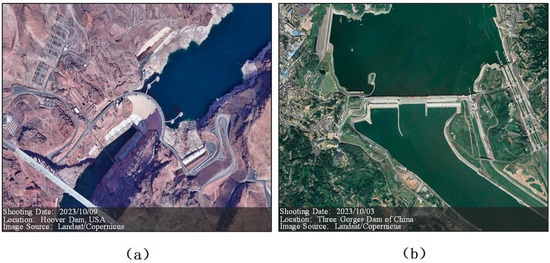
Figure 4.
Dams in Remotely sensed Images (Image Source: Landsat/Copernicus), ((a) depicts the arch-shaped Hoover Dam in the U.S.; (b) showcases the straight-line structure of the Three Gorges Dam in China).
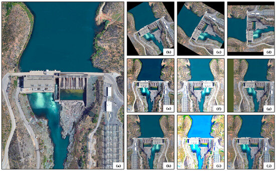
Figure 5.
Schematic representation of the enhancement results for the dam dataset. ((a) Original map, (b) 30 degrees rotation, (c) 60 degrees rotation, (d) 90 degrees rotation, (e) Contrast Enhancement, (f) Brightness Enhancement, (g) Image Panning, (h) Mirror Flip, (i) Add Random Color, (j) Enhancement Color)).
After the sample enhancement process, the dams in it are manually labeled, while in the process of labeling, the quality of the samples is manually checked, screened, and labeled to remove the unqualified samples such as duplicates, deformations, incomplete and unrecognizable objects, etc., and finally, a valid sample set of 4108 sheets is obtained. The labeled sample set is randomly divided into a training sample set and a test sample set, of which 70% are training samples and 30% are validation samples.
Furthermore, the elevation data utilized in this study are sourced from the Advanced Land Observing Satellite (ALOS) project, managed by the Japan Aerospace Exploration Agency (JAXA), which commenced operations in 2006. Specifically, the ALOS-12.5-m resolution elevation data are acquired through the Phased Array type L-band Synthetic Aperture Radar (PALSAR) sensor onboard the ALOS satellite [29]. This sensor offers three distinct observation modes: high resolution, scanning synthetic aperture radar, and polarization. Notably, the ALOS-DEM data boasts horizontal and vertical accuracies of up to 12.5 m, rendering it suitable for generating three-dimensional terrain models. Subsequently, the data are regionally refined by cropping to delineate the elevation data specific to Qinghai Province. Data download at https://search.asf.alaska.edu/ (accessed on 15 October 2023).
2.3. Methods
The technical approach used in this study is illustrated in Figure 6 and is divided into three main phases: Training and testing of the dam dataset using deep learning models: this initial step focuses on training and testing the best weights specifically for dam recognition. Implementing a spatial constraint strategy: A spatial constraint strategy was designed to minimize the interference of external factors. The strategy aims to restrict the analysis to a specified spatial region to minimize the impact of background interfering factors. Integrating deep learning models with a spatial constraining strategy for dam recognition and extraction: integrating deep learning models with spatial constraints strategy helps to accurately recognize and extract dam structures from images. Nomenclature abbreviations are used in the flowchart and detailed names are given in Appendix A.
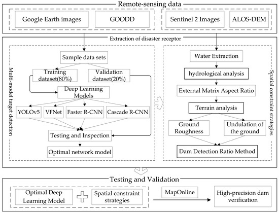
Figure 6.
Flowchart of identification and extraction techniques for a typical hazard-bearing body-dam.
2.3.1. Multi-Model Target Detection
Dam extraction constitutes a pivotal aspect of feature extraction, with recent years witnessing a surge in interest towards deep learning-based target extraction methodologies [30]. Within the realm of feature extraction from remotely sensed imagery, several noteworthy algorithms have emerged, leveraging the inherent advantages of deep learning for target recognition. This section delves into the exploration of four prominent target detection algorithms, seeking to discern their efficacy in the context of extracting typical bearer dams.
There are two primary categories of target recognition models: one-stage and two-stage. One-stage models undertake the simultaneous detection and localization of objects within an image without the necessity of generating additional candidate regions. These models are distinguished by their simplicity and speed, rendering them particularly suitable for real-time detection applications. Prominent examples of one-stage target recognition models encompass YOLO, SSD, and RetinaNet. In contrast, two-stage models partition the target detection task into two distinct phases: the generation of candidate regions and subsequent target classification and localization. Noteworthy examples of two-stage target recognition models encompass Faster R-CNN and R-FCN [16,31,32]. While two-stage models typically exhibit superior accuracy and localization precision, one-stage methods offer expedited processing times.
YOLOv5 is the fifth generation of the YOLO [26] family, which uses a single-stage target detection approach and reformulates the target detection as a regression problem. Its basic architecture consists of an input layer, a backbone network, an intermediate layer, and an output layer. The backbone network is responsible for feature extraction, the intermediate layer is connected using the FPN + PAN structure, and the output layer is responsible for category and location prediction. Various components, such as CBL, SPP, CSP, Focus, Concat, add, and Conv, are integrated for feature processing and fusion. VariFocalNet, on the other hand, is a dense target detection algorithm [33] that extracts feature maps using YOLOv5 as a base model. It uses VariFocal Loss on these feature maps to improve the detection performance and subsequently applies the NMS algorithm in post-processing to eliminate redundant detections. VFNet performs well in a variety of target detection tasks, especially in complex scenes. A distinguishing feature of VFNet lies in its introduction of the ‘multifocal’ mechanism, which enables the model to concentrate on target objects across diverse locations and scales. This multifocal mechanism, coupled with Varifocal Loss, contributes significantly to enhancing the model’s performance across a wide array of targets. VFNet’s multi-focus mechanism and Varifocal Loss bolster the model’s adaptability to a myriad of target scenarios.
Faster R-CNN stands as an advanced deep learning model [16]. It employs a shared convolutional network to construct the Region Proposal Network (RPN) based on the framework of Fast R-CNN, facilitating direct prediction of proposed frames. By extracting image features through a neural network, Faster R-CNN utilizes the RPN to generate multiple candidate target frames. These frames undergo ROI pooling and fully connected operations for target classification and precise localization. Subsequently, the final target detection results undergo non-maximum suppression to filter out redundant detections. This method yields a smaller set of high-quality suggestion frames, significantly enhancing the speed of target recognition. Cascade R-CNN, an extended and refined iteration of Faster R-CNN [34], enhances its predecessor’s capabilities by employing a cascading structure. This structure integrates independent target detectors at each level, which sequentially screen higher-quality candidate frames across multiple detection iterations. At each level, detectors first perform target detection, assigning confidence scores to candidate target regions, and then undergo training using distinct loss functions. Notably, Cascade R-CNN facilitates end-to-end training, allowing detectors at different levels to share feature extractors. This accelerates the training process and refines grading to enhance detection accuracy. Our choice to explore these two distinct models enables us to conduct experimental comparisons, evaluating their performance, strengths, and weaknesses in the context of a specific task—such as the identification of a typical disaster-prone structure like a dam. This analysis not only informs immediate decision-making but also guides future research endeavors.
2.3.2. Spatial Constraint Strategies
- Hydrological analysis. Dams serve as vital hydraulic structures [35], with hydrologic analysis playing a pivotal role in their site selection and design processes. Hydrologic analysis, a scientific method within the realm of Geographic Information Systems (GISs) and hydrology, aims to ascertain the distribution and attributes of river networks through Digital Elevation Models (DEMs) of the study area. Subsequently, it classifies and prioritizes watersheds to pinpoint those with high flow rates. Thus, the precise identification of dam locations necessitates a thorough examination of water bodies. To determine the optimal dam location, the process begins by extracting water body information from remotely sensed imagery utilizing the Normalized Difference Water Body Index (NDWI) [36], as depicted by Equation (1). Following this, the river network within the region is delineated and extracted from DEM data and then categorized and hierarchically subdivided based on factors such as size, geographical positioning, and flow characteristics. It is worth noting that there is a difference in the spatial resolution between the elevation data and the satellite image, and when comparing the two, we have to make the spatial resolution consistent through the resampling method; therefore, we obtain the same resolution as the elevation data by resampling the preprocessed satellite image in ArcGIS, which is 12.5 m. Finally, the external rectangular aspect ratio is computed to identify nodes of disconnection within elongated watersheds. Equation (2) illustrates the formula for calculating the external rectangle aspect ratio (AR), where ‘L’ represents the length of the external rectangle and ‘W’ signifies its width.
- Terrain analysis. When pinpointing the optimal location for a dam, leveraging topographic features becomes imperative. These features furnish critical insights into the geographical landscape, aiding in the precise extraction of dam locations while effectively mitigating the influence of background information. Terrain analysis encompasses two primary facets: ground roughness and ground undulation. Ground roughness quantifies the surface morphology by evaluating the ratio of a raster cell’s surface area to its projected area within a designated region. Denoted by the symbol ‘M,’ ground roughness is computed as the ratio of the surface area of each raster cell (ABAC) to its projected area. Here, in a longitudinal section of a raster cell (ABC), ‘α’ represents the slope of the sub-raster cell. The surface area of AB (ABAC) divided by the projected area of the cell (AC) is expressed by cosα = AC/AB, as detailed in Equation (3). On the other hand, the degree of ground undulation serves as a quantitative measure describing the morphology of landforms. It denotes the maximum relative elevation difference per unit area. This parameter, symbolized by ‘R’, is computed using Equation (4), where ‘Hmax’ represents the maximum elevation value per unit area, and ‘Hmin’ represents the minimum elevation value per unit area.
- Dam Detection Ratio Method. The Dam Detection Ratio Method (DDRM) method is a GIS analysis method for long watershed analysis and water body feature identification. The core idea is to determine the presence or absence of dams by analyzing nodes in the watershed based on the spatial distribution of water body features. The method takes the center point of the dam candidate area as the origin, establishes appropriate buffer zones around it, and determines whether the candidate area is a dam or not by the ratio of the water area on both sides of the dam candidate area. This provides important information about water resources and topographic features. The DDRM calculation formula is shown in Equation (5). Within a certain range of buffer zones, Sp denotes the result of the progressive ratio, U denotes the larger of the watershed areas in the buffer zone, and D denotes the smaller of the watershed areas in the buffer zone.
2.3.3. Evaluation Methodology
The experiment was conducted on the Windows Operating System platform (OS), the graphics card was AMD Ryzen 7 (CPU) and NVIDIA GeForce RTX4060 graphics card (GPU), and the deep learning framework was Python3.9, Pytorch1.12.1. The training started with the initialization of weights on the model, and the parameter settings were shown in Table 2.
Table 2.
Four Deep Learning Model Hyperparameter Settings.
In the typical bearer-dam identification task, the performance of each deep learning model is evaluated based on accuracy, recall, and inference speed (FPS), as shown in Table 3. Accuracy represents the ratio of dam bounding boxes correctly detected by the model to the total number of detected bounding boxes, and recall represents the ratio of dams correctly identified by the model in the validation dataset to the total number of dams actually present. The formulas for precision, recall, and AP (average precision) are as follows:
Table 3.
Four Deep Learning Model Hyperparameter Settings.
Precision–Recall (P-R) curves illustrate the fluctuation of precision and recall under different Intersection of Union (IoU) thresholds. The bounding region of these curves is called Average Precision (AP), which is a composite metric that takes into account both the detection precision and completeness of the model under different IoU thresholds. As shown in Figure 7, a higher AP value indicates that the model is more capable of providing highly accurate detection results under different IoU thresholds. Notably, the cascaded R-CNN has a relatively small variance and has the largest area under two IoU thresholds, indicating its ability to reliably recognize targets under different conditions. However, despite the advances brought about by deep learning models, there are inherent limitations, as shown in Figure 2. Deep learning models tend to misclassify bridges, roads, and reservoir dams as dams. Distinguishing dams from these structures through deep learning recognition methods alone is challenging. Therefore, spatial constraint strategies must be integrated to reduce such confounding factors and improve recognition accuracy.
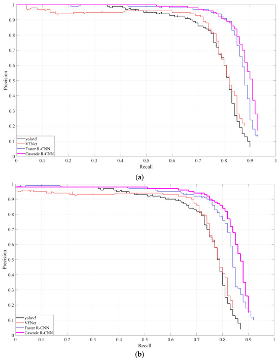
Figure 7.
P-R curves for four deep learning models ((a) IOU = 0.50, (b) IOU = 0.75).
The dams extracted in this chapter result in point-type vectors, and this section uses three indicators, namely, extraction rate, omission rate, and false extraction rate, to comprehensively evaluate the extraction effect of various models. The extraction rate indicates the ratio of the number of dams correctly extracted to the true number of dams, and the formula is shown in Equation (10) where E is the extraction rate, R is the number of dams correctly extracted, and T is the true number of dams. The omission rate indicates the ratio of the number of dams not extracted to the true number of dams, and the formula is shown in Equation (11) where M is the omission rate, R is the number of dams correctly extracted, and T is the true number of dams. False extraction rate represents the ratio of the number of dams incorrectly extracted to the true number of dams, and the formula is shown in Equation (12) where F is the false extraction rate, k is the number of dams incorrectly extracted, and T is the true number of dams.
3. Results
3.1. Spatial Constraint Strategy
3.1.1. Results of Hydrological Analysis
In Figure 8a, the water body extracted from the preprocessed remotely sensed image using the threshold segmentation method is depicted. Figure 8b shows the classification of the river network generated by the Digital Elevation Model (DEM) through ArcGIS, which is divided into seven levels by flow size according to the guidelines of the International Commission on Dams (ICDs). Notably, dams are typically constructed where river volume is substantial, yet areas with the highest river volume are often unsuitable for dam construction. Consequently, our study primarily concentrates on rivers classified as classes 3, 4, 5, and 6, with additional insights to be gleaned from the examination of class 1 and 2 rivers. Given that dams intersect rivers, resulting in discontinuities in the water body delineated via remotely sensed imagery, we employed an external matrix aspect ratio to identify breaks in the watershed. This approach enables us to specifically target rivers within the region, excluding roads and reservoir embankments. Figure 8c illustrates all identified breakpoints along the main stem watersheds within the study area.
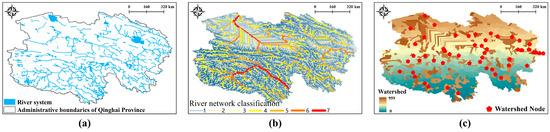
Figure 8.
Results of hydrological analysis ((a) river system, (b) river network classification, (c) watershed nodes)).
3.1.2. Results of Terrain Analysis
Based on conventional knowledge of dams, it becomes apparent that ground roughness and undulation are more pronounced in dam areas (see (1) and (3) in Figure 9b), whereas they are comparatively reduced in urban regions (see (2) and (4) in Figure 9b). Leveraging this disparity, we can utilize ground roughness and undulation metrics to effectively mitigate interference from irrelevant point locations. Figure 9a, c offers a visual juxtaposition of the outcomes of terrain analysis before and after processing, respectively. This comparison underscores the utility of terrain analysis in refining the discrimination range further.
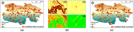
Figure 9.
Results of hydrological analysis ((a) dam candidate area before terrain analysis, (b) terrain analysis process, and (c) dam candidate area after terrain analysis)).
3.1.3. Dam Testing Ratio Test Results
The approach involves calculating the ratio of water area on both sides of the dam. A threshold, often set to one in the experiments, determines whether the target is considered a dam. This threshold can be adjusted based on the completeness of the water portion in the original dam image, allowing for progressive relaxation. For the dam investigation, it is crucial to compute the area ratio upstream and downstream of the dammed river, particularly within a 500-m buffer zone from the dam. If the upstream area ratio closely resembles the downstream area ratio (refer to Figure 10b), it suggests the absence of a dam. Conversely, if the upstream area ratio surpasses one (as illustrated in Figure 10a), it indicates the potential presence of a dam. Furthermore, bridges can be eliminated based on Digital Dam Removal Models (DDRMs). Table 4 showcases points with a ratio of one, which can be omitted based on the comparison of water area ratios on both sides of the river at each point.
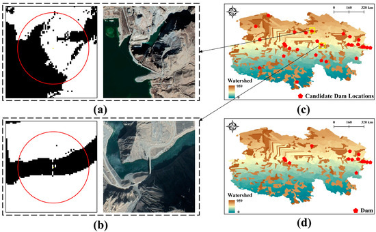
Figure 10.
Water area ratio Water area ratio. ((a) indicates upstream and downstream water bodies that are not similar in size within the red circular buffer zone; (b) indicates upstream and downstream water bodies of similar size within the red circular buffer zone; (c) and (d) indicates pre-screening and post-screening results).
Table 4.
Results of the ratio of the area of waters on both sides of the river at different points.
3.2. Model Evaluation
Using these comprehensive performance metrics, we assess the results presented in Table 5 and Table 6, which illustrate the performance of the four deep learning models in the dam extraction task. It is evident that all models exhibit relatively low extraction rates, a phenomenon that can be attributed to various factors. This underscores the challenge of achieving optimal performance with a single model when confronted with a complex task. However, upon integrating the spatial constraints strategy, a notable enhancement in extraction performance is observed, as depicted in Table 5. The experimental findings underscore the active role of the spatial constraint strategy in addressing the extraction task, offering an effective approach for typical hazard-bearing body-dam extraction. To gain deeper insights into the practical applicability of these four models, we opt to visualize their extraction results, as demonstrated in Figure 11.
Table 5.
Dam extraction rate, leakage rate, and false extraction rate for deep learning models.
Table 6.
Dam extraction rate, leakage rate and false extraction rate after method fusion.
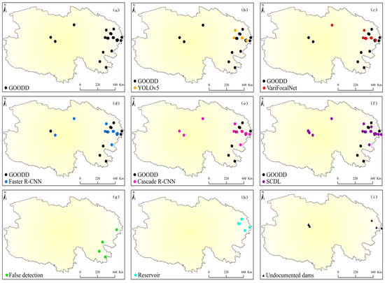
Figure 11.
Visualization results ((a) Dams in the database, (b) YOLOv5 recognition results, (c) VariFocalNet recognition results, (d) Faster R-CNN recognition results, (e) Cascade R-CNN recognition results, (f) Enhanced luminance of the recognition results of SCDL, (g) Misdetection (h) Reservoirs, (i) Unrecorded dams).
In Figure 11, a comprehensive view of the performance of various deep learning models in the dam extraction task is presented: (a) the image displays the point vector dam locations in the GOODD database, serving as a benchmark for our study and objectively verifying the accuracy of SCDL extraction. In Figure 11, (b), (c), (d), and (e) showcase the recognition outcomes by four deep learning models on the dam locations depicted in (a). A comparative analysis reveals that the CascadeR-CNN model exhibits superior performance in dam recognition, demonstrating a notably higher accuracy than other models. In Figure 11, (f) illustrates the recognition effectiveness of the SCDL model, which integrates the best single deep learning model with a spatial constraint strategy. Results indicate a substantial enhancement in the accuracy of typical hazard-bearing body-dam extraction following the incorporation of spatial constraints. Remarkably, a comparison between (f) and (a) reveals that the SCDL model successfully identifies unrecorded points in the database. To validate the model’s performance, ArcMap is utilized for point matching validation, yielding the following results: (g) and (h) showcase points in the database erroneously detected as dam reservoirs, indicating misclassifications. (i), conversely, represents dams detected by the model that are absent in the database. This signifies that the SCDL model not only enhances accuracy but also identifies new dam locations, offering valuable insights for database refinement and updates.
4. Discussion
4.1. Model Comparison and Spatial Constraint Strategy Expansion Analysis
In this study, the extraction method combining deep learning and spatial constraint strategies successfully extracted the dams in the study area. In order to verify the reasonableness of the method proposed in this paper, we compared the extraction rate and accuracy of the four models at the same time, where accuracy refers to the proportion of the extraction rate that is correct. As shown in Table 7, Varifocal Net has the lowest extraction rate among the single model comparisons, but the highest accuracy rate; similarly, the network still has the highest accuracy rate among the coupled models, but the network has a lower omission rate. In a comprehensive comparison, Cascade R-CNN performs well in both extraction rate and accuracy. By comparing the single model and the coupled model, we find that the extraction rate and accuracy of the coupled model are higher than those of the single model, which implies that the spatial constraint strategy can assist the deep learning model to improve the detection performance.
Table 7.
Dam extraction rate and accuracy of deep learning models.
The primary objective of employing the spatial constraint strategy is to confine the geographical extent of the target. Within the dam extraction process, this strategy encompasses hydrologic analysis, topographic analysis, and the implementation of a dam scale detection method. It is worth noting that the composition of spatial constraint strategies may show differences for different disaster-bearing bodies. Under different disaster scenarios, the characteristics and spatial distribution of disaster-bearing bodies may be diverse [37]. Consequently, it is imperative to adapt the spatial constraints strategy composition flexibly to suit different disaster-bearing bodies. For instance, in the extraction of a common disaster-bearing body like a house, the spatial constraint strategy may be constructed using topographic analysis [38], land use classification [39], and building characterization. By synergistically applying these spatial constraints, the expectation is to achieve a more precise identification of various types of disaster-bearing bodies, effectively narrowing down the discrimination range. This approach aims to facilitate the accurate localization and identification of specific target types in remote-sensing images.
4.2. Analysis of Sub-Watershed Hazard-Bearing Bodies
In our extraction process, our primary focus was on experimenting with rivers at the large watershed level. However, it is crucial to note that dams also exist in smaller watersheds, as illustrated in Figure 12. In this figure, b, e, and h represent dams within small watersheds, while a, d, and g correspond to the water bodies in those dam areas. Additionally, c, f, and i depict the corresponding topographic landforms in the dam area. Upon analyzing water bodies and topographic features, it becomes evident that the accuracy of dam extraction is heavily influenced by the effectiveness of water body extraction [40,41] and the precision of the terrain model generated by DEM [42,43,44]. Inaccurate water body extraction can lead to the omission of dams, thereby compromising extraction accuracy. A high-quality DEM contributes to a more accurate terrain model, capturing subtle changes in the area, including small topographic features and variations in surface elevation. Conversely, a low-accuracy DEM may result in blurred or overlooked details, presenting a terrain model with flatter and simplified features.
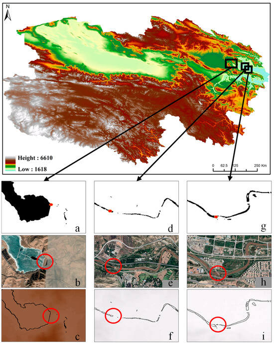
Figure 12.
Analysis of sub-watershed receptors. ((a,d,g) representing the spatial distribution of water bodies on both sides of the dam; (b,e,h) indicates the actual view of each dam in the red buffer zone; (c,f,i) depicts the corresponding topography of the dam area within the red buffer zone).
4.3. Limitations of DDRM
The effectiveness of the DDRM method hinges on the spatial distribution of water body features, demanding a high level of stability in these features. However, this stability can vary significantly across different environments. Factors such as seasonality and climate change may induce notable fluctuations in the shape and size of water bodies, introducing challenges to the accuracy of the DDRM method and potentially resulting in misclassifications. Moreover, the DDRM method necessitates an appropriate buffer zone for calculating the watershed area ratio. Nevertheless, determining the size of this buffer zone often relies on subjective judgment or trial-and-error methods, as depicted in Figure 13. This variability may lead different researchers to employ distinct buffer zone settings in various contexts, thereby impacting the consistency and reproducibility of results. In our experiments, we assumed that a dam is identified when the upstream/downstream area ratio exceeds one, based on the spatial feature distribution of water on both sides of the dam. However, in practical scenarios, as illustrated in Figure 14, there may be a dam where the area ratio on the two sides is not greater than one. Consequently, the area ratio threshold could potentially be set at alternative values, such as 0.65, 0.75, or 0.85.
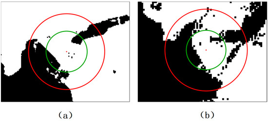
Figure 13.
Buffer zones with different thresholds. ((a,b) represent the spatial distribution of water bodies on either side of the dam in the buffer zone, green buffer has a radius of 300 m, red buffer has a radius of 500 m).
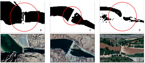
Figure 14.
Dams present in sub-basins. ((a,c,e) indicates dams of similar size upstream and downstream in the red circular buffer zone; (b,d,f) the actual view of each dam is represented separately).
5. Conclusions
Within the existing disaster management system, conducting a thorough census and implementing efficient management of disaster-bearing entities are recognized as fundamental stages in disaster risk assessment and zoning. Ensuring the quality and completeness of pertinent data are crucial for accurately delineating areas at risk of disasters, optimizing resource allocation, and formulating effective strategies for disaster response.
In this study, we tackle the challenge posed by the difficulty of a single remotely sensed image extraction method in distinguishing between similar features. To address this, we propose an extraction method that combines deep learning and spatial constraint strategies. This approach involves comparing spatial features of dams with those of similar features, like bridges, roads, and reservoir embankments. By carefully selecting appropriate constraint strategies, establishing separability index rules for dams and the mentioned features, and employing hydrological analyses to narrow the research scope to the river, interference from roads and reservoir embankments can be excluded. Additionally, terrain analysis is utilized to eliminate interference from bridges. The accuracy of the extraction results for a typical disaster-bearing entity—dams—is evaluated using three indicators: extraction rate, omission rate, and false extraction rate.
The accuracy of dam extraction is contingent not only on the precision of the neural network but also on factors such as image quality, the effectiveness of water body extraction, and post-processing accuracy. Our dataset comprises high-quality dam images encompassing various types, sizes, and geographic locations. The accuracy of image quality and class not only enhances the performance of the deep learning model but also elucidates the texture and morphological features of dams more clearly. The introduction of DDRM in this study was pivotal in narrowing down the dam discrimination range. This effectively eliminated interfering point locations within the study area, making significant contributions to the accurate extraction of dam candidates. The hybrid method, combining deep learning and spatial constraint strategies, not only identifies typical disaster-bearing entities but also successfully pinpoints dam locations. The method achieves high accuracy, with extraction rates, omission rates, and false extraction rates of 94.73%, 5.27%, and 11.11%, respectively. Our findings indicate that, built upon open geographic data products, the proposed technological process in this paper demonstrates reliability in dam extraction and effectively identifies and locates targets. This approach not only overcomes the limitations and challenges of traditional methods but also uncovers dams not recorded in the database, offering new insights and possibilities for the management, monitoring, and planning of typical hazard-bearing bodies.
This study serves as a valuable reference for the methodology and implementation of dam target detection using open geographic data and technology. While some progress has been achieved in this research direction, there are still potential challenges and areas for improvement. On one hand, the model’s training dataset could be further refined to enhance its generalization ability, and the integration of more advanced recognition models may contribute to further improvements in dam recognition performance. On the other hand, exploring additional high-resolution remotely sensed data sources could enhance the accuracy of dam recognition. Furthermore, considering the application of the framework on a global scale and in other fields could help address challenges in global dam management and geological research. This broader application could play a role in contributing to the sustainable development of human society.
Author Contributions
Conceptualization, L.W. and Q.C.; methodology, L.W.; software, L.W.; validation, L.W., Y.X. and Q.C.; formal analysis, L.W. and Q.C.; investigation, L.W.; resources, J.W.; data curation, L.W.; writing—original draft preparation, L.W.; writing—review and editing, J.L. (Jianhui Luo), X.L., R.P. and J.L. (Jiaxin Li); visualization, L.W.; supervision, Q.C.; project administration, L.W.; funding acquisition, Y.X. All authors have read and agreed to the published version of the manuscript.
Funding
This research was funded by THE NATIONAL KEY R&D PLAN OF China, grant number 2022YFC3004404, 2023YFF1305303.
Institutional Review Board Statement
Not applicable.
Informed Consent Statement
Not applicable.
Data Availability Statement
The data that support the findings of this study are available from the author upon reasonable request. The data are not publicly available due to privacy restrictions.
Conflicts of Interest
The authors declare no conflicts of interest.
Appendix A
| Abbreviated Nouns | Interpretation of Nouns |
| GOODD | The Global Geo-Referenced Database of Dams |
| YOLO | You Only Look Once (That is the full name of what we often refer to as a YOLO) |
| VFNET | VarifocalNet (VF-Net) A target detection network |
| R-CNN | Region-based Convolutional Neural Network (A Deep Learning Model for Object Detection) |
| ALOS-DEM | ALOS-DEM data, elevation data acquired by the ALOS (Advanced Land Observing Satellite. Launched in 2006) satellite phased-array L-band synthetic aperture radar (PALSAR) |
| SCDL | Remotely sensed Recognition Method Based on Deep Learning and Spatial Constraint Strategy |
| SCS | Spatial constraint strategy |
| DDRM | Digital Dam Removal Models |
| IOU | Intersection of Union |
| AP | Average Precision |
Appendix B
| Band Number | Band Name | Central Wavelength (nm) | Spatial Resolution (m) |
| 1 | Coastal aerosol | 443 | 60 |
| 2 | Blue | 490 | 10 |
| 3 | Green | 560 | 10 |
| 4 | Red | 665 | 10 |
| 5 | Vegetation red edge | 705 | 20 |
| 6 | Vegetation red edge | 740 | 20 |
| 7 | Vegetation red edge | 783 | 20 |
| 8 | NIR Narrow | 842 | 10 |
| 8A | NIR Narrow | 865 | 20 |
| 9 | Water vapor | 945 | 60 |
| 10 | SWIR | 1375 | 60 |
| 11 | SWIR | 1610 | 20 |
| 12 | SWIR | 2190 | 20 |
References
- Gao, C.; Zhang, B.; Shao, S.; Hao, M.; Zhang, Y.; Xu, Y.; Kuang, Y.; Dong, L.; Wang, Z. Risk assessment and zoning of flood disaster in Wuchengxiyu Region, China. Urban Clim. 2023, 49, 101562. [Google Scholar] [CrossRef]
- Jia, L.; Wang, J.; Gao, S.; Fang, L.; Wang, D. Landslide risk evaluation method of open-pit mine based on numerical simulation of large deformation of landslide. Sci. Rep. 2023, 13, 15410. [Google Scholar] [CrossRef]
- Feng, D.; Shi, X.; Renaud, F.G. Risk assessment for hurricane-induced pluvial flooding in urban areas using a GIS-based multi-criteria approach: A case study of Hurricane Harvey in Houston, USA. Sci. Total Environ. 2023, 904, 166891. [Google Scholar] [CrossRef] [PubMed]
- Qiao, W.; Shen, L.; Wen, Q.; Wen, Q.; Tang, S.; Li, Z. Revolutionizing building damage detection: A novel weakly supervised approach using high-resolution remote sensing images. Int. J. Digit. Earth 2023, 17, 2298245. [Google Scholar] [CrossRef]
- Tavra, M.; Lisec, A.; Galešić Divić, M.; Cetl, V. Unpacking the role of volunteered geographic information in disaster management: Focus on data quality. Geomat. Nat. Hazards Risk 2024, 15, 2300825. [Google Scholar] [CrossRef]
- Jing, M.; Cheng, L.; Ji, C.; Mao, J.; Li, N.; Duan, Z.; Li, Z.; Li, M. Detecting unknown dams from high-resolution remote sensing images: A deep learning and spatial analysis approach. Int. J. Appl. Earth Obs. Geoinf. 2021, 104, 102576. [Google Scholar] [CrossRef]
- Zhang, H.; Li, Q.; Wang, J.; Fu, B.; Duan, Z.; Zhao, Z. Application of Space–Sky–Earth Integration Technology with UAVs in Risk Identification of Tailings Ponds. Drones 2023, 7, 222. [Google Scholar] [CrossRef]
- Sebasco, N.P.; Sevil, H.E. Graph-Based Image Segmentation for Road Extraction from Post-Disaster Aerial Footage. Drones 2022, 6, 315. [Google Scholar] [CrossRef]
- Han, X.; Wang, J. Earthquake Information Extraction and Comparison from Different Sources Based on Web Text. ISPRS Int. J. Geo-Inf. 2019, 8, 252. [Google Scholar] [CrossRef]
- Li, S.T.; Song, W.W.; Fang, L.Y.; Chen, Y.S.; Ghamisi, P.; Benediktsson, J.A. Deep Learning for Hyperspectral Image Classification: An Overview. IEEE Trans. Geosci. Remote Sens. 2019, 57, 6690–6709. [Google Scholar] [CrossRef]
- Guo, J.; Jia, N.; Bai, J. Transformer based on channel-spatial attention for accurate classification of scenes in remote sensing image. Sci. Rep. 2022, 12, 15473. [Google Scholar] [CrossRef] [PubMed]
- Biffi, L.J.; Mitishita, E.; Liesenberg, V.; dos Santos, A.A.; Gonçalves, D.N.; Estrabis, N.V.; Silva, J.D.; Osco, L.P.; Ramos, A.P.M.; Centeno, J.A.S.; et al. ATSS Deep Learning-Based Approach to Detect Apple Fruits. Remote Sens. 2021, 13, 54. [Google Scholar] [CrossRef]
- Balaniuk, R.; Isupova, O.; Reece, S. Mining and Tailings Dam Detection in Satellite Imagery Using Deep Learning. Sensors 2020, 20, 6936. [Google Scholar] [CrossRef] [PubMed]
- Ghanbari, H.; Mahdianpari, M.; Homayouni, S.; Mohammadimanesh, F. A Meta-Analysis of Convolutional Neural Networks for Remote Sensing Applications. IEEE J. Sel. Top. Appl. Earth Obs. Remote Sens. 2021, 14, 3602–3613. [Google Scholar] [CrossRef]
- Shao, J.N.; Yang, Q.Y.; Luo, C.Y.; Li, R.H.; Zhou, Y.S.; Zhang, F.X. Vessel Detection From Nighttime Remote Sensing Imagery Based on Deep Learning. IEEE J. Sel. Top. Appl. Earth Obs. Remote Sens. 2021, 14, 12536–12544. [Google Scholar] [CrossRef]
- Yan, D.C.; Li, G.Q.; Li, X.Q.; Zhang, H.; Lei, H.; Lu, K.X.; Cheng, M.H.; Zhu, F.X. An Improved Faster R-CNN Method to Detect Tailings Ponds from High-Resolution Remote Sensing Images. Remote Sens. 2021, 13, 2052. [Google Scholar] [CrossRef]
- Kahar, S.; Hu, F.; Xu, F. Ship Detection in Complex Environment Using SAR Time Series. IEEE J. Sel. Top. Appl. Earth Obs. Remote Sens. 2022, 15, 3552–3563. [Google Scholar] [CrossRef]
- Liu, X.; Xu, L.; Zhang, J. Landslide detection with Mask R-CNN using complex background enhancement based on multi-scale samples. Geomat. Nat. Hazards Risk 2024, 15, 2300823. [Google Scholar] [CrossRef]
- van Soesbergen, A.; Chu, Z.D.; Shi, M.J.; Mulligan, M. Dam Reservoir Extraction From Remote Sensing Imagery Using Tailored Metric Learning Strategies. IEEE Trans. Geosci. Remote Sens. 2022, 60, 4207414. [Google Scholar] [CrossRef]
- Asbury, Z.; Aly, M.H. A geospatial study of the drought impact on surface water reservoirs: Study cases from Texas, USA. Gisci. Remote Sens. 2019, 56, 894–910. [Google Scholar] [CrossRef]
- Yang, Y.; Shao, Z.P.; Hu, Y.; Mei, Q.; Pan, J.C.; Song, R.X.; Wang, P. Geographical spatial analysis and risk prediction based on machine learning for maritime traffic accidents: A case study of Fujian sea area. Ocean. Eng. 2022, 266, 113106. [Google Scholar] [CrossRef]
- Chen, L.K.; Zhong, Q.K.; Li, Z. Analysis of spatial characteristics and influence mechanism of human settlement suitability in traditional villages based on multi-scale geographically weighted regression model: A case study of Hunan province. Ecol. Indic. 2023, 154, 110828. [Google Scholar] [CrossRef]
- Mulligan, M.; van Soesbergen, A.; Saenz, L. GOODD, a global dataset of more than 38,000 georeferenced dams. Sci. Data 2020, 7, 31. [Google Scholar] [CrossRef] [PubMed]
- Steve Keyamfe Nwagoum, C.; Yemefack, M.; Silatsa Tedou, F.B.; Tabi Oben, F. Sentinel-2 and Landsat-8 potentials for high-resolution mapping of the shifting agricultural landscape mosaic systems of southern Cameroon. Int. J. Appl. Earth Obs. Geoinf. 2023, 124, 103545. [Google Scholar] [CrossRef]
- Lin, C.; Guo, S.; Chen, J.; Sun, L.; Zheng, X.; Yang, Y.; Xiong, Y. Deep Learning Network Intensification for Preventing Noisy-Labeled Samples for Remote Sensing Classification. Remote Sens. 2021, 13, 1689. [Google Scholar] [CrossRef]
- Mujahid, A.; Awan, M.J.; Yasin, A.; Mohammed, M.A.; Damaševičius, R.; Maskeliūnas, R.; Abdulkareem, K.H. Real-Time Hand Gesture Recognition Based on Deep Learning YOLOv3 Model. Appl. Sci. 2021, 11, 4164. [Google Scholar] [CrossRef]
- Geng, L.; Meng, Q.; Xiao, Z.; Liu, Y. Measurement of Period Length and Skew Angle Patterns of Textile Cutting Pieces Based on Faster R-CNN. Appl. Sci. 2019, 9, 3026. [Google Scholar] [CrossRef]
- de Carvalho, O.L.F.; de Carvalho Júnior, O.A.; Silva, C.R.e.; de Albuquerque, A.O.; Santana, N.C.; Borges, D.L.; Gomes, R.A.T.; Guimarães, R.F. Panoptic Segmentation Meets Remote Sensing. Remote Sens. 2022, 14, 965. [Google Scholar] [CrossRef]
- Weifeng, X.; Jun, L.; Dailiang, P.; Jinge, J.; Hongxuan, X.; Hongyue, Y.; Jun, Y. Multi-source DEM accuracy evaluation based on ICESat-2 in Qinghai-Tibet Plateau, China. Int. J. Digit. Earth 2023, 17, 2297843. [Google Scholar] [CrossRef]
- Hu, L.; Niu, C.; Ren, S.; Dong, M.; Zheng, C.; Zhang, W.; Liang, J. Discriminative Context-Aware Network for Target Extraction in Remote Sensing Imagery. IEEE J. Sel. Top. Appl. Earth Obs. Remote Sens. 2022, 15, 700–715. [Google Scholar] [CrossRef]
- Li, J.; Liang, X.; Shen, S.; Xu, T.; Feng, J.; Yan, S. Scale-aware Fast R-CNN for Pedestrian Detection. IEEE Trans. Multimed. 2017, 20, 985–996. [Google Scholar] [CrossRef]
- Liu, Q.; Hang, R.; Song, H.; Li, Z. Learning Multiscale Deep Features for High-Resolution Satellite Image Scene Classification. IEEE Trans. Geosci. Remote Sens. 2018, 56, 117–126. [Google Scholar] [CrossRef]
- Huang, C.L.; Zhang, Z.F.; Zhang, X.J.; Jiang, L.; Hua, X.D.; Ye, J.L.; Yang, W.N.; Song, P.; Zhu, L.F. A Novel Intelligent System for Dynamic Observation of Cotton Verticillium Wilt. Plant Phenomics 2023, 5, 13. [Google Scholar] [CrossRef]
- Zhang, X.; Han, L.X.; Robinson, M.; Gallagher, A. A Gans-Based Deep Learning Framework for Automatic Subsurface Object Recognition From Ground Penetrating Radar Data. IEEE Access 2021, 9, 39009–39018. [Google Scholar] [CrossRef]
- Barbarossa, V.; Schmitt, R.J.P.; Huijbregts, M.A.J.; Zarfl, C.; King, H.; Schipper, A.M. Impacts of current and future large dams on the geographic range connectivity of freshwater fish worldwide. Proc. Natl. Acad. Sci. USA 2020, 117, 3648–3655. [Google Scholar] [CrossRef] [PubMed]
- Zhang, G.; Yao, T.; Chen, W.; Zheng, G.; Shum, C.K.; Yang, K.; Piao, S.; Sheng, Y.; Yi, S.; Li, J.; et al. Regional differences of lake evolution across China during 1960s–2015 and its natural and anthropogenic causes. Remote Sens. Environ. 2019, 221, 386–404. [Google Scholar] [CrossRef]
- Sun, L.; Wang, Q.; Chen, Y.; Zheng, Y.; Wu, Z.; Fu, L.; Jeon, B. CRNet: Channel-Enhanced Remodeling-Based Network for Salient Object Detection in Optical Remote Sensing Images. IEEE Trans. Geosci. Remote Sens. 2023, 61, 5618314. [Google Scholar] [CrossRef]
- Safanelli, J.; Poppiel, R.; Ruiz, L.; Bonfatti, B.; Mello, F.; Rizzo, R.; Demattê, J. Terrain Analysis in Google Earth Engine: A Method Adapted for High-Performance Global-Scale Analysis. ISPRS Int. J. Geo-Inf. 2020, 9, 400. [Google Scholar] [CrossRef]
- Zhang, H.K.; Roy, D.P. Using the 500 m MODIS land cover product to derive a consistent continental scale 30 m Landsat land cover classification. Remote Sens. Environ. 2017, 197, 15–34. [Google Scholar] [CrossRef]
- Li, X.; Zhang, F.; Chan, N.W.; Shi, J.; Liu, C.; Chen, D. High Precision Extraction of Surface Water from Complex Terrain in Bosten Lake Basin Based on Water Index and Slope Mask Data. Water 2022, 14, 2809. [Google Scholar] [CrossRef]
- Chen, C.; Liang, J.; Liu, Z.; Xu, W.; Zhang, Z.; Zhang, X.; Chen, J. Method of Water Body Information Extraction in Complex Geographical Environment from Remote Sensing Images. Sens. Mater. 2022, 34, 4325–4338. [Google Scholar] [CrossRef]
- Moges, D.M.; Virro, H.; Kmoch, A.; Cibin, R.; Rohith, A.N.; Martinez-Salvador, A.; Conesa-Garcia, C.; Uuemaa, E. How does the choice of DEMs affect catchment hydrological modeling? Sci. Total Environ. 2023, 892, 164627. [Google Scholar] [CrossRef] [PubMed]
- Xu, K.; Fang, J.; Fang, Y.; Sun, Q.; Wu, C.; Liu, M. The Importance of Digital Elevation Model Selection in Flood Simulation and a Proposed Method to Reduce DEM Errors: A Case Study in Shanghai. Int. J. Disaster Risk Sci. 2021, 12, 890–902. [Google Scholar] [CrossRef]
- Sukumaran, H.; Sahoo, S.N. A Methodological Framework for Identification of Baseline Scenario and Assessing the Impact of DEM Scenarios on SWAT Model Outputs. Water Resour. Manag. 2020, 34, 4795–4814. [Google Scholar] [CrossRef]
Disclaimer/Publisher’s Note: The statements, opinions and data contained in all publications are solely those of the individual author(s) and contributor(s) and not of MDPI and/or the editor(s). MDPI and/or the editor(s) disclaim responsibility for any injury to people or property resulting from any ideas, methods, instructions or products referred to in the content. |
© 2024 by the authors. Licensee MDPI, Basel, Switzerland. This article is an open access article distributed under the terms and conditions of the Creative Commons Attribution (CC BY) license (https://creativecommons.org/licenses/by/4.0/).