Estimation and Evaluation of 15 Minute, 40 Meter Surface Upward Longwave Radiation Downscaled from the Geostationary FY-4B AGRI

Abstract

Surface upward longwave radiation (SULR) is one of the four components of surface net radiation. Geostationary satellites can provide high temporal but coarse spatial resolution SULR products. Downscaling coarse SULR to a higher resolution is important for fine-scale thermal condition monitoring. Statistical regression downscaling is widely used due to its simplicity and is built on the assumption that the thermal parameter like land surface temperature (LST) or SULR has a relationship with the related surface factors like the normalized difference vegetation index (NDVI), and the relationship remains unchanged in any scales. In this study, to establish the relationship between SULR and the related surface factors, we chose the multiple linear regression (MLR) model and five surface factors (i.e., the modified normalized difference water index (MNDWI), normalized difference built-up and soil index (NDBSI), NDVI, normalized moisture difference index (NMDI), and urban index (UI)) to drive the downscaling process. Additionally, a step-by-step downscaling strategy was applied to reach the 100-fold increase in spatial resolution, transitioning the estimated SULR from 4 km of the advanced geostationary radiation imager (AGRI) onboard FengYun-4B (FY-4B) satellite to 40 m of the visual and infrared multispectral imager (VIMI) in infrared spectrum onboard GaoFen5-02 (GF5-02). Finally, we evaluated the downscaling results by comparing the downscaled SULR values with the in situ measured SULR and GF5-02-calculated SULR, and the root mean square errors (RMSEs) were 19.70 W/m² and 24.86 W/m², respectively. Throughout this MLR-based step-by-step downscaling method (high-frequency data from FY-4B and high spatial resolution data from GF5-02), high spatiotemporal SULR (15 min temporal resolution, 40 m spatial resolution) were successfully generated instead of coarse spatial resolution ones from the FY-4B satellite or a coarse temporal resolution one from the GF5-02 satellite, relieving the above-mentioned conflict to some extent.

1. Introduction

Land surface energy balance is central to any land model that characterizes land surface processes and is depicted using net radiation. Surface upward longwave radiation (SULR) is an important component of all-wave net radiation, which includes shortwave and longwave net radiation components [1,2,3]. SULR is defined as the sum of the radiation emitted from the land surface and the first-order reflected component of surface downward longwave radiation (SDLR) [4]. SULR with high spatiotemporal resolution can greatly enhance the understanding of atmospheric circulations like hydrological and meteorological cycles [5], land surface processes like surface matter–energy exchange [6,7], thermal condition monitoring [8,9], agricultural applications, and even global climate change [10]. Remote sensing is a promising technology that can estimate SULR on a global or regional scale. However, the products derived from thermal infrared remote sensing often face challenges in terms of conflicting spatial and temporal resolutions. For instance, the land surface temperature (LST) product of the moderate resolution imaging spectroradiometer (MODIS) onboard Terra and Aqua satellites offers four observations at most during a day but is limited to a spatial resolution of only 1000 m in the infrared spectrum. The spatial resolution of the Landsat thermal infrared sensor (TIRS) is 100 m, but its revisit period is 16 days. The advanced geostationary radiation imager (AGRI) onboard the FengYun-4B (FY-4B) satellite, on the other hand, provides a high temporal resolution with a 15 min revisit time but has a coarser spatial resolution of 4 km in the infrared spectrum. For the visual and infrared multispectral imager (VIMI) onboard GaoFen5-02 (GF5-02), the spatial resolution of its infrared bands is 40 m, and its revisit time is up to 51 days. This conflict commonly exists and seriously hinders the utilization of remote-sensing products.

To improve the spatial resolution of satellite-derived products, statistical regression downscaling methods have been developed and widely used due to their consideration of thermal infrared radiation and their low computational complexity [11,12,13,14,15,16]. The statistical regression method is based on the assumption of “scale consistence”, which posits that physical parameters like LST and LST-related factors such as the normalized difference vegetation index (NDVI), exhibit a statistical regression relationship that remains consistent regardless of the spatial scale. By utilizing regression factors with greater spatial texture information, the spatial resolution of the physical parameter (LST) can be improved. This kind of method was designed early on for vegetation-covered areas [17,18] using a linear regression model and single surface factor (e.g., NDVI), limiting the application scenarios. Over time, the approach has evolved to incorporate multiple linear regression (MLR) models, enhancing the robustness of the fitted relationship and expanding the applicability to various land cover types [19]. With the increase in remote sensing data and the development of regression models, nonlinear regression techniques such as machine learning have become popular choices for describing surface physical conditions and establishing complex relationships between LST and regression factors. For instance, Hutengs and Vohland [20] constructed a nonlinear relationship between LST and surface factors using a random forest (RF), improving the spatial resolution of MODIS LST products from 1000 m to 250 m. Zihao et al. employed back propagation neural networks to downscale LST products, achieving a spatial resolution of 30 m for Landsat thermal infrared images with an original resolution of 100 m, showcasing their potential ability for complex background areas [21]. Dong et al. integrated kernel-based and fusion-based downscaling methods with RF regression techniques, successfully downscaling MODIS LST from 1000 m to 100 m spatial resolution in alignment with Landsat 8/9 images [22].

However, these methods are generally implemented within a relatively small-scale span of approximately 10–20 times [18,19,20,21,22,23]. As the scale span increases, traditional statistical regression downscaling methods tend to perform poorly, which is attributed to the discrepancy in the assumption of scale–relationship consistency. Thus, the effectiveness of directly statistical downscaling methods for much larger spans (such as 100 times from 4 km of FY-4B to 40 m of GF5-02) remains unclear. To perform large-span downscaling, the step-by-step method based on LST was proposed to conduct downscaling in adjacent scales with a small span, ensuring the validity of the scale–relationship consistency assumption [24,25]. On the other hand, these downscaling methods primarily focus on LST, and their suitability for SULR remains uncertain, even though these two parameters both show thermal conditions. Therefore, a comprehensive evaluation of a large-span downscaling method for SULR is necessary. This study aims to achieve the following two main objectives: (1) to estimate the 4km SULR and downscale to 40 m (aligning with FY-4B and GF5-02) and (2) to evaluate the accuracy of large-span (100 times) downscaled results using in-situ measurement validation and GF5-02 cross-comparison.

The structure of this paper is organized as follows: Section 2 introduces the study area and provides information on the remotely sensed data from the FY-4B and GF5-02 satellites. Section 3 presents the downscaling methodology using the MLR model with a step-by-step strategy, detailed with the original SULR estimation, surface factor selection, and step-by-step downscaling process. The downscaling results and a comparative analysis are included in Section 4. Finally, conclusions and discussions are presented in Section 5.

2. Study Area and Data

2.1. Study Area

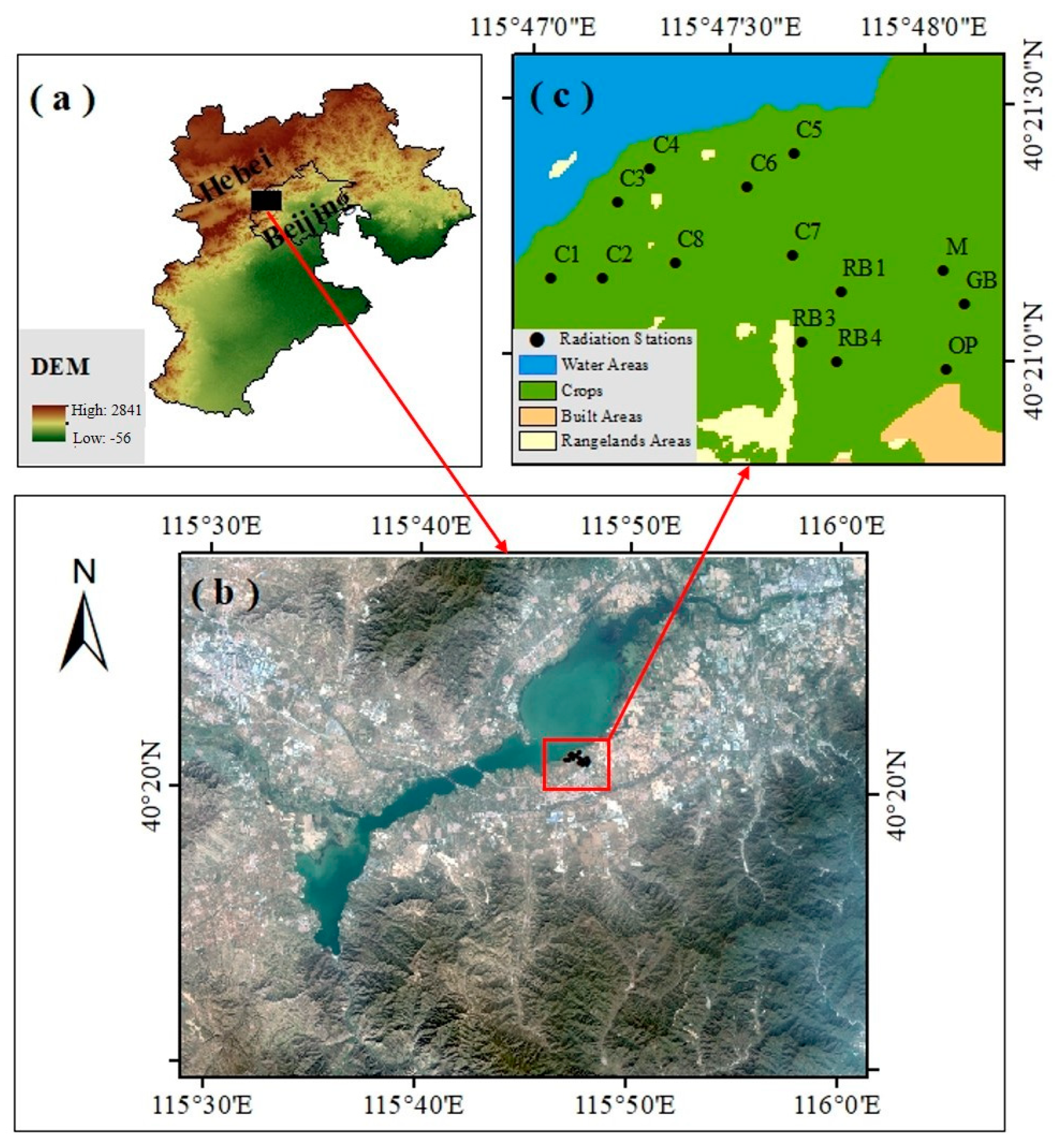
The Huailai Remote Sensing Comprehensive Experiment Station, affiliated with the Chinese Academy of Sciences, is situated on the border between Beijing and the Hebei Province. This station is surrounded by diverse land cover types, including farmland, waterbodies, mountains, grassland, and wetlands. The selection of such a study area allowed for the comprehensive consideration of complex backgrounds and abundant components that contribute to the land surface radiation budget. Additionally, to support the evaluation of the downscaling method, 14 ground radiation stations were strategically placed across the area. The 14 stations were each equipped with one Kipp and Zonen CGR3 net radiometer, which had a spectral wavelength of 4.5–42 μm, a field of view of 150°, and an accuracy of 1 W/m² after the blackbody-based calibration.

These radiometers collect measurements of SULR and SDLR at 10 min intervals, providing reliable validation data for the downscaling process. Figure 1 illustrates the study area and the distribution of the radiation stations.

2.2. Data

2.2.1. GaoFen5-02 VIMI Data

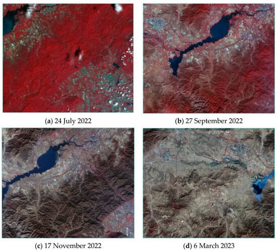
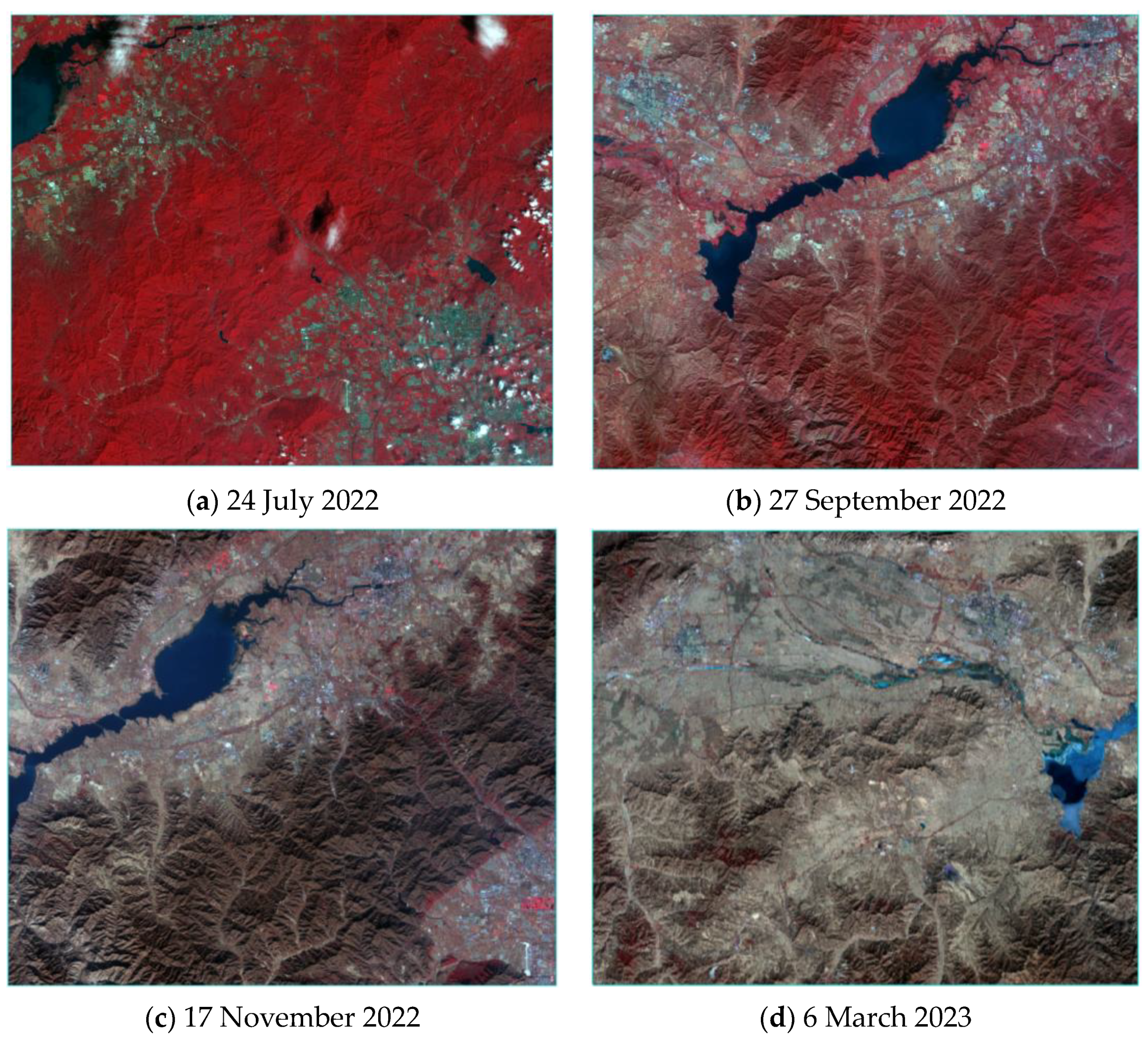
GF5-02 was successfully launched on 7 September 2021 at 11:01 and has since provided a wealth of high-quality remote sensing image data. The data utilized in this study was from the VIMI sensor onboard the GF5-02 satellite. This sensor captures imagery with a width of 60 km and offers two distinct spatial resolutions, depending on the spectral band. In the visible spectrum, the spatial resolution is 20 m, while in the thermal infrared spectrum, it is 40 m. The surface reflectance from GF5-02 VIMI after radiometric calibration and atmospheric correction served to calculate the surface factors to drive the downscaling process, and the thermal infrared data was used to estimate the SULR and compare it with the downscaled SULR results. We tried to select more GF5-02 VIMI images of the study area, but the collected data was scarce due to the long revisit period of GF5-02 and the serious influence of cloud contamination. We finally obtained four images, as shown in Figure 2, which was from 24 July 2022, 27 September 2022, 17 November 2022, and 6 March 2023. In addition, the observation area did not completely overlap when the GF5-02 satellite revisited the study area, which meant that the 14 stations were not included on 6 March 2023. Therefore, the validation method based on in-situ measured SULR was only carried out in three days: 24 July 2022, 27 September 2022, and 17 November 2022.

2.2.2. FengYun-4B AGRI Level 1 Data

The FengYun-4 series of meteorological satellites is the second-generation geostationary meteorological satellite of China, designed as an upgrade of the first-generation geostationary orbit meteorological satellite (FY-2). The FY-4B satellite was launched on 3 June 2021, and started providing data from 1 June 2022. One of the key instruments onboard FY-4B is the AGRI, which offers improved temporal and spatial resolution compared to its predecessor. AGRI observed the study area every 15 min, and it provided thermal infrared data with a subsatellite point spatial resolution of approximately 4 km. In this study, we downloaded the FY-4B AGRI 4 km level 1 full disk data for four specific days, which were 24 July 2022, 27 September 2022, 17 November 2022, and 6 March 2023, consistent with the available GF5-02 data across four seasons from https://satellite.nsmc.org.cn/portalsite/Data/Satellite.aspx accessed on 26 July 2023. The AGRI level 1 data was used to estimate the original SULR in this study. Every day, there were approximately 90 effective data images available, generating the same amount of SULR for downscaling.

3. Methodology

The SULR estimation method, downscaling model and driving factors, and step-by-step downscaling strategy are introduced in Section 3.1, Section 3.2, and Section 3.3, respectively. The evaluation strategy is provided in Section 3.4.

3.1. Hybrid Algorithm for Estimating SULR

SULR is the sum of the thermal radiation emitted by a surface and the reflected SDLR. To retrieve the SULR from remote sensing data, state-of-the-art methods can be categorized into two main approaches: the temperature-broadband emissivity physical method [4,9,26] and the hybrid method [2,27,28]. The temperature-broadband emissivity physical method estimates SULR by utilizing the LST, broadband emissivity, and SDLR. On the other hand, the hybrid method establishes a direct relationship between SULR and the radiances measured via satellite sensors at the top of the atmosphere. This method bypasses the temperature emissivity separation process and generally achieves high accuracy [3,29]. We employed the widely-used linear regression hybrid method with the input of top-of-atmosphere radiances, abbreviated as TOA-LIN [29], to estimate the SULR from the FY-4B and GF5-02 satellites (see Equations (1) and (2)). The key to this method is to accurately calibrate the coefficients. Here, the coefficients of TOA-LIN were derived from simulated datasets including seven typical view zenith angles (VZAs) of 0° to 60° with a step of 10°, 946 atmospheric profiles, 6 LSTs from −10 K to 15 K with a step of 5 K, 35 typical emissivity spectrums including water bodies, vegetation, soil, minerals, ice, snow, and spectral response functions of the 12–14 FY-4B bands as well as the 9–12 GF5-02 bands [29] according to the center wavelength of the thermal infrared spectrums.

$$SUL{R}_{FY}=a_0+a_1\ast R_{12}+a_2\ast R_{13}+a_3\ast R_{14}$$

(1)

where a₀–a₃ denote the calibrated coefficients, and R₁₂–R₁₄ denote the radiance values of the 12, 13, and 14 bands of the FY-4B satellite, respectively.

$$SUL{R}_{GF}=b_0+b_1\ast R_9^{\prime }+b_2\ast R_{10}^{\prime }+b_3\ast R_{11}^{\prime }+b_4\ast R_{12}^{\prime }$$

(2)

Equally, b₀–b₄ denote the calibrated coefficients and $R_9^{\prime }–R_{12}^{\prime }$ denote the radiance values of the 9, 10, 11, and 12 bands of the GF5-02 satellite, respectively.

Consequently, the calibrated coefficients for the 0° to 60° VZAs were obtained and are presented in

Table 1. Calibrated coefficients to estimate the SULR of the FY-4B and GF5-02 satellites at VZA = 0–60° with a 10° step.

	VZA	0°	10°	20°	30°	40°	50°	60°
FY-4B AGRI	a0	86.0905	86.4723	87.6620	89.7995	93.1742	98.3240	106.2046
	a1	−2.4927	−2.5541	−2.7384	−3.0441	−3.4589	−3.9184	−4.1643
	a2	105.9331	106.7086	109.0992	113.3028	119.7131	129.0193	142.3019
	a3	−68.9081	−69.7235	−72.2442	−76.7023	−83.5696	−93.7132	−108.6330
	RMSE (W/m2)	6.65	6.71	6.91	7.27	7.86	8.82	10.48
GF5-02 VIMI	b0	−38.0897	−38.4436	−39.5298	−41.4500	−44.4164	−48.8187	−55.5221
	b1	21.8166	22.0164	22.6375	23.7702	25.6111	28.5709	33.6638
	b2	104.2309	104.8645	106.8184	110.2269	115.3711	122.7523	132.9230
	b3	−53.2957	−53.8959	−55.7607	−59.0569	−64.1387	−71.6837	−82.6188
	b4	66.9902	67.2557	68.0969	69.6449	72.1708	76.1867	82.4844
	RMSE (W/m2)	6.03	6.09	6.26	6.59	7.13	8.05	9.65

. The SULR for a specific VZA could be calculated with the coefficients of two adjacent VZAs via interpolation. The selected TOA-LIN hybrid method in this study had an acceptable accuracy (with an RMSE of approximately less than 10 W/m²).

3.2. Surface Factors and Downscaling the Model Selection

Surface factors play a critical role as driving kernels in providing spatial information for downscaling purposes [30]. These factors encompass a wide range of thermal-related parameters, ranging from visual and near-infrared spectrums to shortwave infrared spectrums. They also include terrain and land-cover type factors specific to the scenes being studied. For instance, Sánchez et al. downscaled the Sentinel-3 LST to Sentinel-2 resolution with only the NDVI in a specific agriculture area [31]. Zhu et al. employed a NDVI, digital elevation model (DEM), slope, latitude, and longitude to describe the distribution and variation of the LST, downscaling the MODIS LST to a 100 m resolution in an area with a complex landscape [32]. To clarify how to select the thermal-related factors to drive the different downscaling processes, Dong et al. conducted a comprehensive comparison of thirty-five statistical regression downscaling LST algorithms (seven scaling factors × five regression models) across thirty-two geographical regions worldwide. They concluded that a RF with approximately 30–50 scaling factors or MLR with approximately six factors had the highest accuracy [30]. Here, we chose MLR as the regression model, considering that our study area consisted of only 120 pixels (10 rows × 12 columns) at a 4 km scale, which is insufficient for training a RF model. Furthermore, given the various landscapes in the study area (water bodies, vegetation, soil, and urban areas), we selected the following five surface factors: (1) the modified normalized difference water index (MNDWI), highlighting the water bodies in the study area; (2) the normalized difference built-up and soil index (NDBSI), providing information about the soil and building coverage; (3) the NDVI, describing the vegetation cover condition in the study area; (4) the normalized moisture difference index (NMDI), indicating the vegetation moisture, and (5) the urban index (UI), providing urban information in the study area. These factors effectively characterized the property of the entire study area, as listed in

Table 2. The definitions, descriptions, and formulas of the surface factors.

Index	Description	Formula
MNDWI	Improves the normalized difference water body index to highlight water	$\frac{B2-B6}{B2+B6}$
NDBSI	Indicates the degree of dryness of the ground surface	$IBI=\frac{\frac{2\ast B5}{B5+B4}-(\frac{B4}{B4+B3}+\frac{B2}{B2+B5})}{\frac{2\ast B5}{B5+B4}+(\frac{B4}{B4+B3}+\frac{B2}{B2+B5})}$ $SI=\frac{\left(B5+B3\right)-(B4+B1)}{\left(B5+B3\right)+(B4+B1)}$ $NDBSI=\frac{IBI+SI}{2}$
NDVI	Highlights the vegetation information	$\frac{B4-B3}{B4+B3}$
NMDI	Indicates the vegetation moisture	$\frac{B4-(B5-B6)}{B4+(B5+B6)}$
UI	Highlights the urban information	$\frac{B6-B4}{B6+B4}$

Notes: B1–B6 denote the surface reflectance of band 1–band 6 of the GaoFen5-02 satellite, which are 0.440–0.510, 0.510–0.580, 0.620–0.680, 0.760–0.870, 1.540–1.700, and 2.060–2.350 µm, respectively.

. The surface reflectance for calculating these factors was obtained after the radiometric calibration and atmospheric correction of the GF5-02 original data. The MLR with the input of the selected factors is provided in Section 3.3.

3.3. MLR-Based Step-by-Step Downscaling Strategy

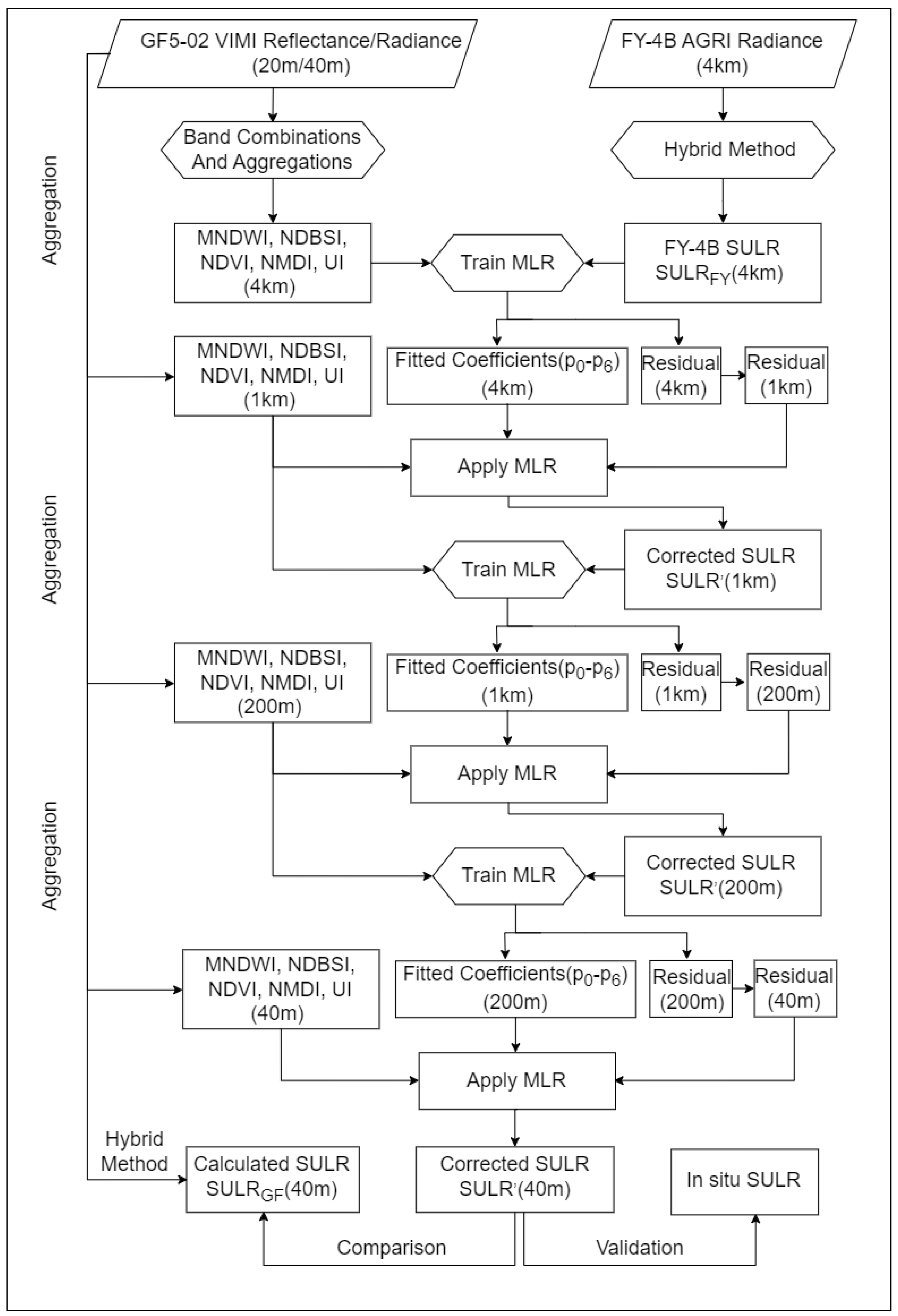
The statistical regression downscaling method is based on the assumption that the relationship between the SULR and surface factors remains unchanged across different spatial scales. However, as the scale difference increases, especially in regions with strong spatial heterogeneity, the downscaled results perform worse. To solve this problem, the step-by-step downscaling strategy was introduced [24,25], which establishes and applies the relationship between the SULR and surface factors in every two adjacent scales. Theoretically, the intermediate resolutions could be any number between the initial and target resolutions. In this study, we selected 1 km and 200 m as the intermediate scales, performing the downscaling process in 4–1 km, 1 km–200 m, and 200–40 m steps since a too-large or small adjacent scale resolution difference leads to a weakened scale effect or redundant computation according to the pre-study test.

As shown in the overall flow chart (Figure 3), in the first-level downscaling from 4 km to 1 km, we initially calculated the MNDWI, NDBSI, NDVI, NMDI, and UI at a 20 m resolution using GF5-02 VIMI reflectance data as introduced in Section 3.2 and resampled them to a 4 km resolution to match the FY-4B SULR, which was estimated using the hybrid method introduced in Section 3.1. Here, we adopted the widely applied areal average method to aggregate the five selected factors into multiple intermediate scales to drive the step-wise downscaling processes, which has been proven to be reliable in previous studies [22,33]. The selected MLR was adopted to build the relationship between the SULR and surface factors in a coarse resolution and then was applied to the next finer resolution according to Equations (3) and (4), respectively.

$${\mathrm{S}\mathrm{U}\mathrm{L}\mathrm{R}}_{\mathrm{c}}={{\mathrm{p}}_0+\mathrm{p}}_1\ast {\mathrm{M}\mathrm{N}\mathrm{D}\mathrm{W}\mathrm{I}}_{\mathrm{c}}+{\mathrm{p}}_2\ast {\mathrm{N}\mathrm{D}\mathrm{B}\mathrm{S}\mathrm{I}}_{\mathrm{c}}+{\mathrm{p}}_3\ast {\mathrm{N}\mathrm{D}\mathrm{V}\mathrm{I}}_{\mathrm{c}}+{\mathrm{p}}_4\ast {\mathrm{N}\mathrm{M}\mathrm{D}\mathrm{I}}_{\mathrm{c}}+{\mathrm{p}}_5\ast {\mathrm{U}\mathrm{I}}_{\mathrm{c}}$$

(3)

$${\mathrm{S}\mathrm{U}\mathrm{L}\mathrm{R}}_f={{\mathrm{p}}_0+\mathrm{p}}_1\ast {\mathrm{M}\mathrm{N}\mathrm{D}\mathrm{W}\mathrm{I}}_{\mathrm{f}}+{\mathrm{p}}_2\ast {\mathrm{N}\mathrm{D}\mathrm{B}\mathrm{S}\mathrm{I}}_{\mathrm{f}}+{\mathrm{p}}_3\ast {\mathrm{N}\mathrm{D}\mathrm{V}\mathrm{I}}_{\mathrm{f}}+{\mathrm{p}}_4\ast {\mathrm{N}\mathrm{M}\mathrm{D}\mathrm{I}}_{\mathrm{f}}+{\mathrm{p}}_5\ast {\mathrm{U}\mathrm{I}}_{\mathrm{f}}$$

(4)

where p₀–p₅ denote the fitted coefficients of MLR; subscript c and f denote the coarse-spatial-resolution and next finer-spatial-resolution, such as the 4 km scale and 1 km scale, respectively.

In the downscaling process from a 4 km to a 1 km scale, it is necessary to ensure that the average value of every 4 × 4 pixels at the 1 km spatial resolution is equivalent to that at the 4 km spatial resolution (i.e., energy balance). Therefore, the unavoidable residual (ΔSULR_c, see Equation (5)) between the original SULR_c and re-aggerated SULR ($\mathrm{S}\mathrm{U}\mathrm{L}{\mathrm{R}}_{\mathrm{f}\to \mathrm{c}}$) needs to be allocated back to the downscaled image [18].

$$\Delta {\mathrm{S}\mathrm{U}\mathrm{L}\mathrm{R}}_c={\mathrm{S}\mathrm{U}\mathrm{L}\mathrm{R}}_{\mathrm{c}}-\mathrm{S}\mathrm{U}\mathrm{L}{\mathrm{R}}_{f\to c}$$

(5)

We resampled the ΔSULR_c using nearest-neighbor interpolation to fine resolution ($\Delta {\mathrm{S}\mathrm{U}\mathrm{L}\mathrm{R}}_{\mathrm{c}\to \mathrm{f}}$) aiming to allocate the residual. To ensure both the energy balance and visual effectiveness, we employed a mean filter with a window size of 3 × 3 to smooth the resampled residual. Then, the smoothed residual was added back to the primary downscaled SULR for generating the corrected fine-spatial-resolution SULR at 1 km (the ${\mathrm{S}\mathrm{U}\mathrm{L}\mathrm{R}}_f^{\prime }$ as shown in Equation (6)).

$${\mathrm{S}\mathrm{U}\mathrm{L}\mathrm{R}}_f^{\prime }={\mathrm{S}\mathrm{U}\mathrm{L}\mathrm{R}}_{\mathrm{f}}+\Delta {\mathrm{S}\mathrm{U}\mathrm{L}\mathrm{R}}_{c\to f}$$

(6)

Subsequently, the MLR function was refitted with the corrected ${\mathrm{S}\mathrm{U}\mathrm{L}\mathrm{R}}_f^{\prime }$ of the 1 km spatial resolution and 1 km surface factors and applied to generate the 200 m SULR. This process was repeated at the 200 m SULR to generate the 40 m SULR, as shown in Figure 3. In summary, we performed the SULR MLR-based step-by-step downscaling method from FY-4B at a 4 km spatial resolution to a 40 m spatial resolution to align with GF5-02 using intermediate scales of 1 km and 200 m.

3.4. Evaluation Strategy

In this study, we adopted two strategies to evaluate the downscaling accuracy: (1) an in situ validation. As introduced in the study area and study data, we had 14 radiation stations collecting SULR every 10 min. We also obtained extensive downscaled images in terms of the high-frequency (every 15 min) property of the FY-4B geostationary satellite data. The in situ measurements were was linearly interpolated to match the FY-4B imaging time. The downscaled 40 m SULR values located in all the radiation stations were extracted, containing approximately 90 pairs every day in each station. It is sufficient to evaluate the downscaling accuracy with these in situ measurements. (2) The calculated SULR comparison. The calculated SULR results from the high-spatial-resolution GF5-02 data allowed an image-to-image assessment of the downscaling effectiveness. Specifically, the downscaled 40 m SULR alignment with the GF5-02 overpass time was compared with the directly calculated SULR from the GF5-02 satellite data using the hybrid method (introduced in Section 3.1). To quantitatively evaluate the accuracy of the downscaling process based on the above two strategies, three metrics containing the root mean square error (RMSE), mean bias error (MBE), and correlation coefficient (R) were employed as the indicators. Equations (7)–(9) were used to calculate these metrics.

$$\mathrm{R}\mathrm{M}\mathrm{S}\mathrm{E}=\sqrt{\frac{1}{n}{\sum _{i=1}^n\left(SUL{R}_{downscaled}-SUL{R}_{reference}\right)}^2}$$

(7)

$$MBE=\frac{1}{n}\sum _{i=1}^n\left(SUL{R}_{downscaled}-SUL{R}_{reference}\right)$$

(8)

$$R=\frac{Cov\left({SULR}_{downscaled},{SULR}_{reference}\right)}{\sqrt{{Var}_{SUL{R}_{downscaled}}\ast {Var}_{SUL{R}_{reference}}}}$$

(9)

In the above equations, SULR_downscaled denotes the downscaled SULR while SULR_reference denotes the SULR data that was collected in situ from the radiation stations or the calculated SULR from GF5-02. Cov(SULR_downscaled, SULR_downscaled) denotes the covariance of the two parameters and ${Var}_{SUL{R}_{downscaled}}$ and ${Var}_{SUL{R}_{reference}}$ denote the variance of SULR_downscaled and SULR_reference, respectively.

4. Results and Evaluation

The results and evaluations were categorized into four different aspects as seen in

Table 3. Data details in Section 4.

Section	Time
4.1 Step-by-step downscaled SULR results	11:15 in local time on 27 September 2022 (i.e., the same as the GF5-02 imaging time of a specific day) (Figure 4)
4.2 Hour-by-hour downscaled SULR results	08:00, 08:15, 08:30…24:00 on 27 September 2022 00:15, 00:30…07:45 on 28 September 2022 in local time (i.e., the same as the FY-4B imaging time of a specific day) (Figure 5)
4.3 Point-by-point validation using the SULR measured in situ	The same time as in Section 4.2 for all 14 stations separately (Figure 6a–n); The same time as in Section 4.2 for all 14 stations together on 24 July 2022, 27 September 2022, and 17 November 2022 (Figure 6o)
4.4 Image-to-image comparison using the calculated GF5-02 SULR	11:15 in local time on 24 July 2022, 27 September 2022, 17 November 2022, and 6 March 2023 (i.e., the same as all the GF5-02 imaging times of four specific days) (Figure 7)

. The step-by-step downscaled SULR results were based on one local time observation (11:15) on a specific day (Section 4.1). The hour-by-hour results were focused on all the hours of one specific day (Section 4.2). The point-by-point validation was achieved in all local times for three days (Section 4.3). The image-to-image comparison was conducted in one local time (11:15) for all four specific days.

4.1. Step-by-Step Downscaled SULR Results

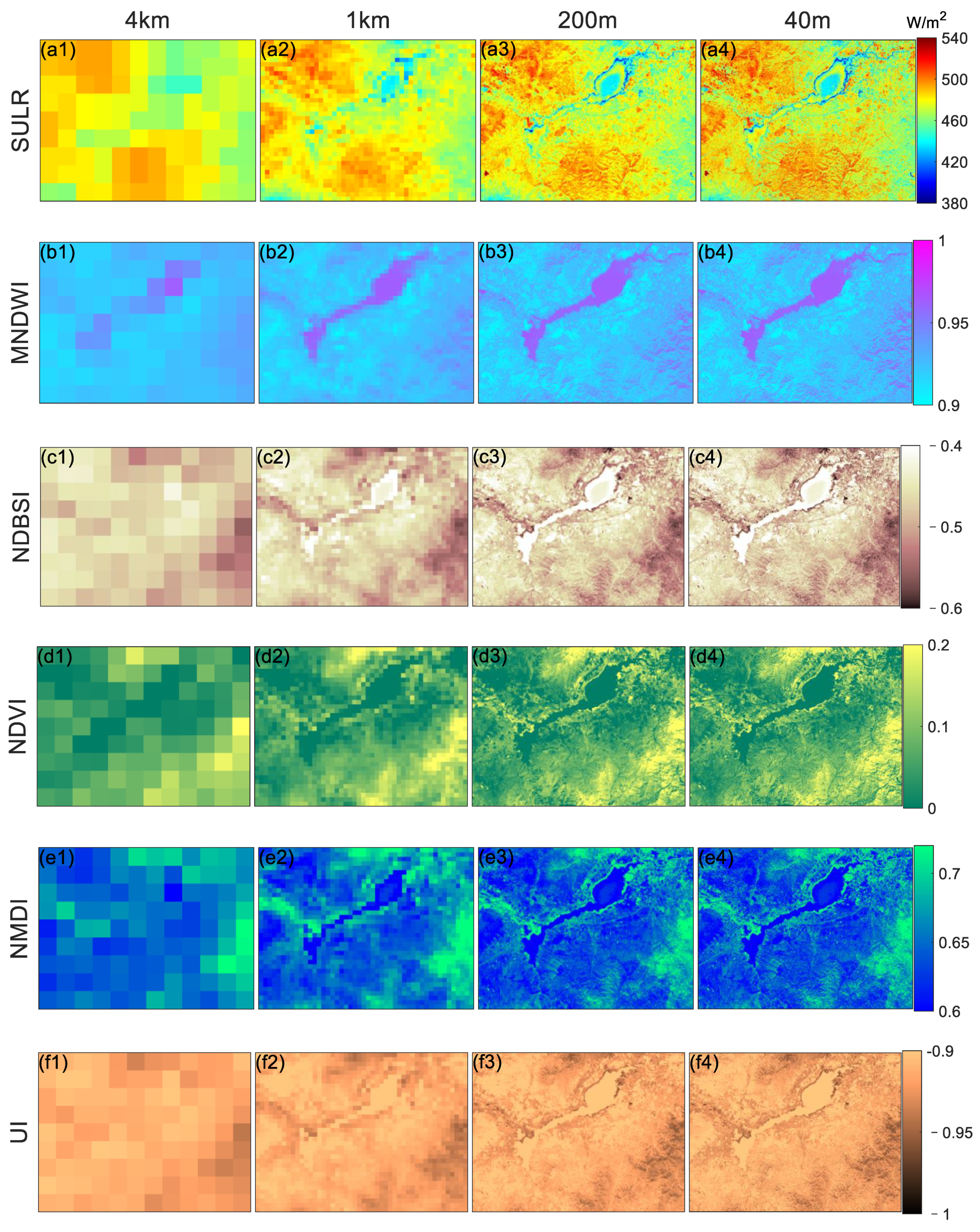
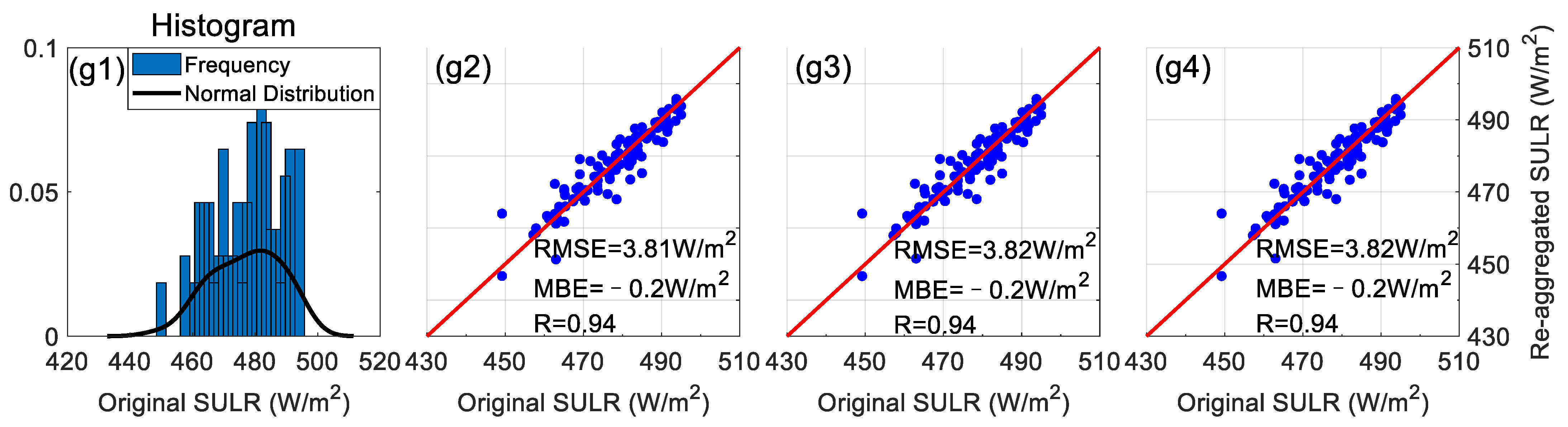
During the step-by-step downscaling process, we progressively obtained the intermediate downscaled SULR images at 1 km, 200 m, and the final result at the 40 m spatial resolution by introducing the surface factors in these scales. The study data from 27 September 2022 (11:15 in local time) was selected as an example to illustrate the following detailed downscaling processes and results. Firstly, Figure 4(a1–f4) exhibits the factors in different scales and the corresponding SULR via downscaling with these factors. As shown in the figure, the spatial texture property gradually recovered through the downscaling processes, demonstrating the successful achievement of step-by-step downscaling. These factors hold a clear texture on their own, contributing to recovering the SULR in higher spatial resolutions. Figure 4(g1) demonstrates the histogram of the originally estimated SULR before downscaling, an approximate range of 440–500 W/m². To validate the preservation of the energy balance during the large-span downscaling process, we conducted a re-aggregation of the downscaled SULR at 1 km, 200 m, and 40 m spatial resolution back to a 4 km spatial resolution and compared the values. This comparison was illustrated in Figure 4(g2–g4) which remains an energy balance in every intermediate scale of step-by-step downscaling with the RMSE between the original SULR and the re-aggregated SULR of 3.82 W/m².

Figure 4. (a1–f4) The intermediate downscaled SULR with the surface factors in the corresponding scales, (g1) the histogram of the original estimated SULR, and (g2–g4) the energy balance during each intermediate-scale downscaling step.

Figure 4. (a1–f4) The intermediate downscaled SULR with the surface factors in the corresponding scales, (g1) the histogram of the original estimated SULR, and (g2–g4) the energy balance during each intermediate-scale downscaling step.

4.2. Hour-by-Hour Downscaled SULR Results

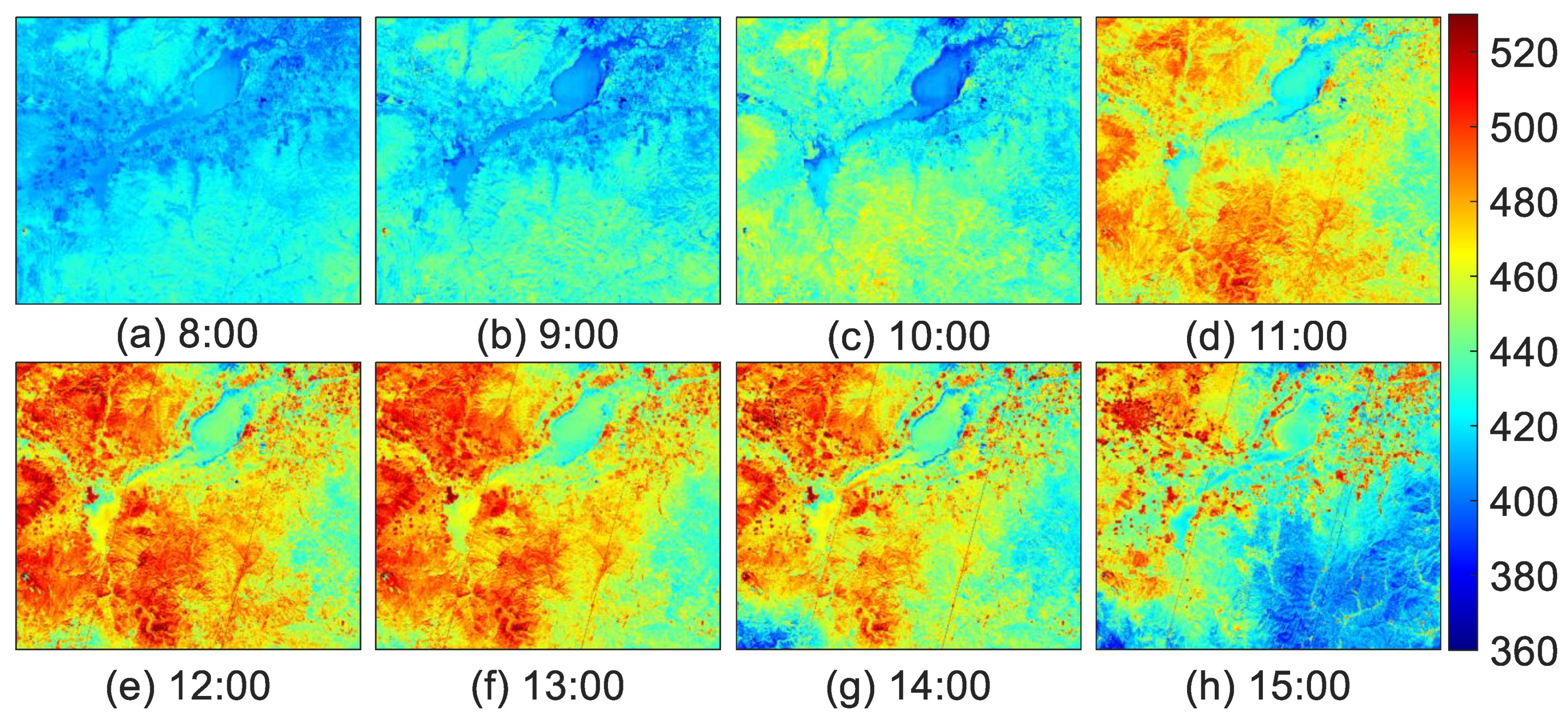
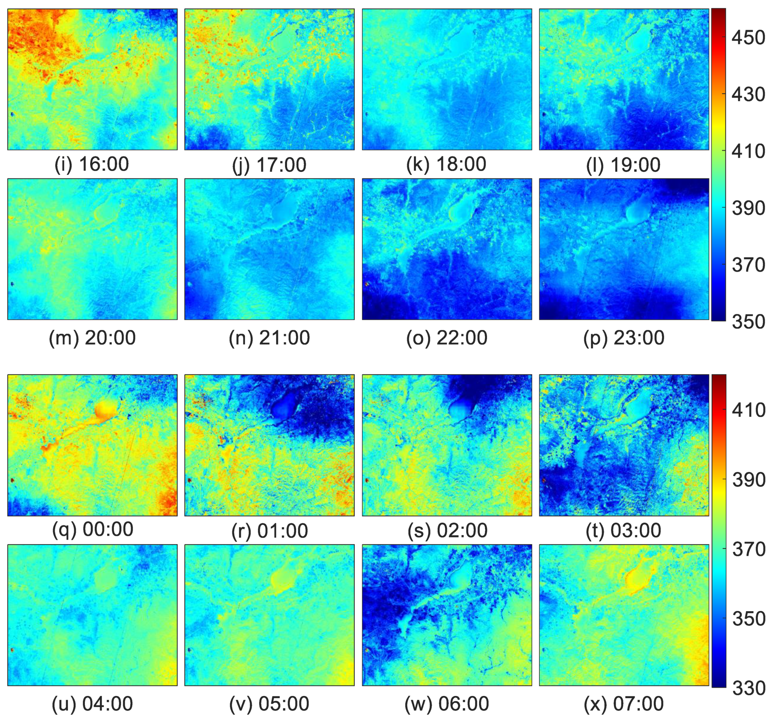
Based on the high-frequency property of the FY-4B data, the MLR-based step-by-step downscaling strategy was applied to the other imaging time on 27 September 2022, generating a high-temporal-resolution SULR dataset that corresponds to the FY-4B original SULR before downscaling. Figure 5 illustrates the downscaled SULR in 24 selected moments of a day based on the local time, revealing a distinct trend with lower SULR values during the nighttime and higher values during the daytime and lower values for waterbodies during the daytime and higher ones during the nighttime.

Figure 5. Downscaled SULR with a resolution of 40 m at 24 moments in an example day (27 September 2022).

Figure 5. Downscaled SULR with a resolution of 40 m at 24 moments in an example day (27 September 2022).

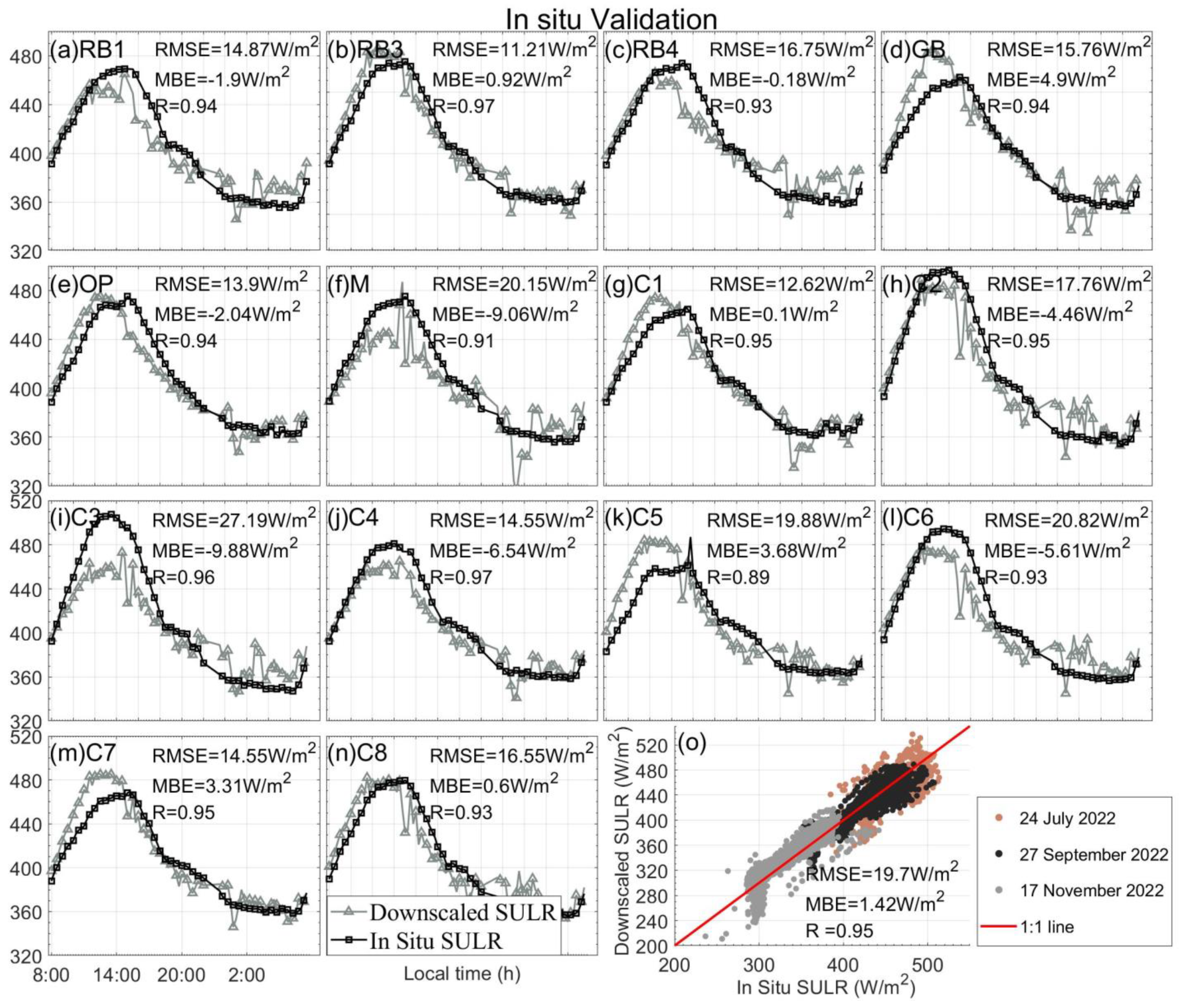
4.3. Point-by-Point Validation Using the SULR Measured In Situ

The SULR collected from 14 radiation stations was employed to quantitatively evaluate the accuracy of the downscaling process based on the above high-temporal-resolution downscaling results. It was difficult to validate SULR in coarse scales using in situ measurements due to the serious spatial heterogeneity in this study area [34]. Therefore, we conducted the point-by-point validation only in the targeted 40 m resolution. According to the latitude and longitude locations of these stations and following the minimum distance principle, we extracted the downscaled SULR values from the entire downscaled image at a 40 m resolution for each station at 15 min intervals, aligning with the temporal resolution of FY-4B. On the example day (27 September 2022), there were 90 effective data images available. Simultaneously, the surface radiation stations collected the SULR values every 10 min, and the interpolation method was adopted to obtain the intermediate SULR values to ensure the temporal resolutions matched. Consequently, 90 pairs of comparisons between the downscaled SULR values and the in situ SULR values were obtained, and the chronological comparison results are presented in Figure 6. The chronological trend exhibits diurnal variation characteristics. On 27 September 2022, the RMSE for 11 out of 14 stations was below 20 W/m², while the average RMSE and MBE for all the stations were 16.90 W/m² and −1.87 W/m², respectively. For 24 July 2022, 27 September 2022, and 17 November 2022, the overall RMSE, MBE, and R of the 14 stations were 19.70 W/m², 1.42 W/m², and 0.95, respectively. These results indicate a favorable downscaling achievement, considering the acceptable instantaneous error of 20 W/m² [35]. Recent SULR estimations have achieved an approximate accuracy with a RMSE from 15.72 to 18.75 W/m², which is very close to the RMSE of our study [36,37,38].

Figure 6. In situ validation for the downscaling process in 14 stations. (a–n) the in situ validation of 14 stations on the example day (27 September 2022) and (o) the validation of all the stations on three study days.

Figure 6. In situ validation for the downscaling process in 14 stations. (a–n) the in situ validation of 14 stations on the example day (27 September 2022) and (o) the validation of all the stations on three study days.

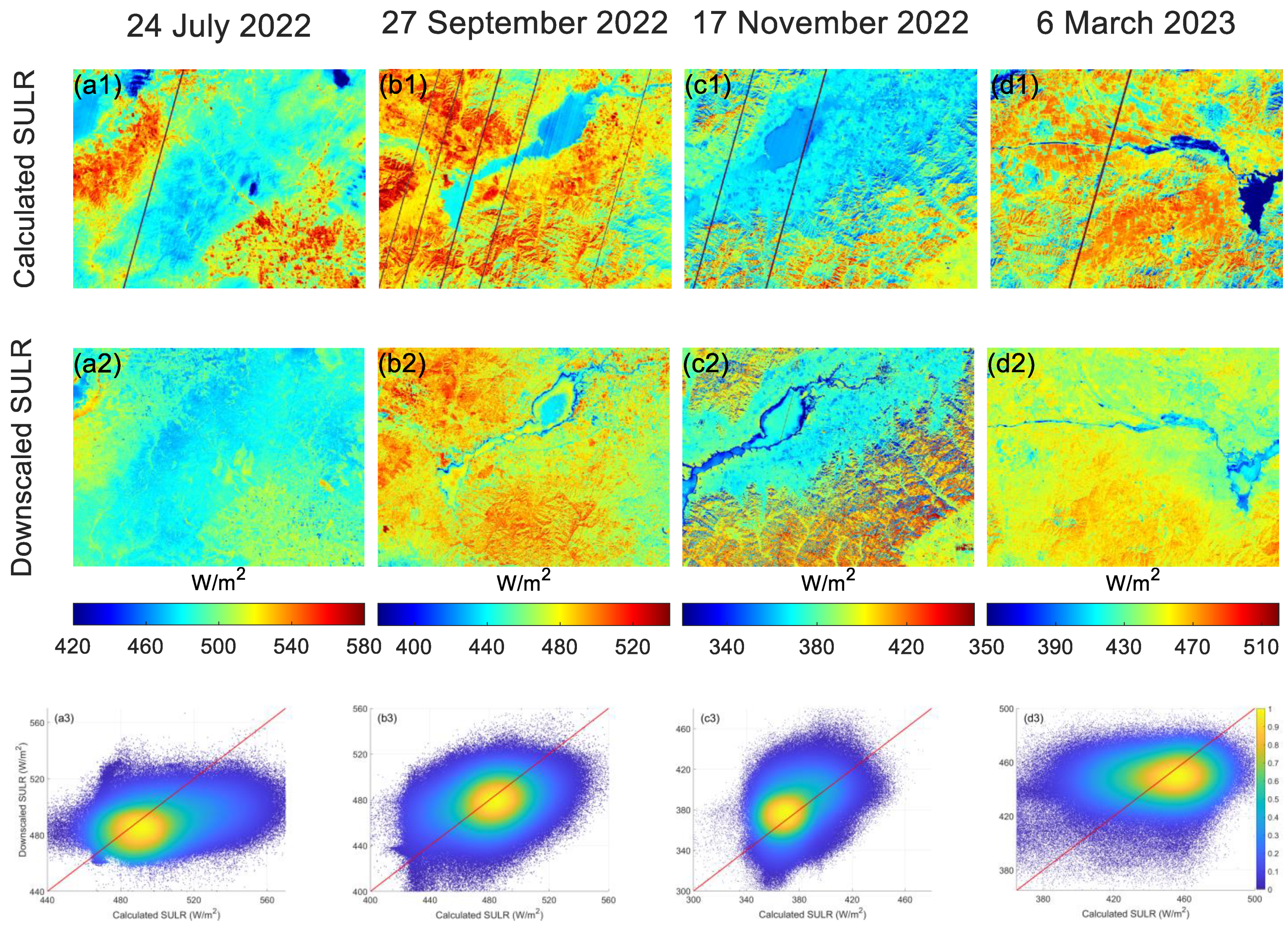
4.4. Image-to-Image Comparison Using the Calculated GF5-02 SULR

Besides the in situ validation, evaluating the downscaling results from an image perspective is necessary. We compared the downscaled SULR with the calculated SULR for each pixel at a 40 m resolution, which was estimated directly from the GF5-02 satellite thermal infrared data using the hybrid method outlined in Section 3.1. The root mean square difference (RMSD) between the GF5-02 calculation and FY-4B downscaling results was approximately 23.21, 24.22, 24.10, and 27.90 W/m² on four study days (see Figure 7 and

Table 4. The RMSD, MBE, and correlation coefficient between the downscaled SULR and calculated SULR.

	24 July 2022	27 September 2022	17 November 2022	6 March 2023
RMSD (W/m2)	23.21	24.22)	24.10	27.90
MBE (W/m2)	−11.46	−3.00	6.53	4.68
R	0.42	0.38	0.41	0.31

). From an image perspective, the downscaled SULR varied in a smaller range than the reference ones with an overestimation in the water body areas and an underestimation in the mountain areas.

Figure 7. Comparison between the GF5-02-calculated SULR and FY-4B-downscaled SULR; (a1–d1) SULRs calculated from the GF5-02 data on four study days; (a2–d2) downscaled SULR of the corresponding days; (a3–d3) comparison results. Table 4 shows the detailed comparison values.

Figure 7. Comparison between the GF5-02-calculated SULR and FY-4B-downscaled SULR; (a1–d1) SULRs calculated from the GF5-02 data on four study days; (a2–d2) downscaled SULR of the corresponding days; (a3–d3) comparison results. Table 4 shows the detailed comparison values.

5. Conclusions and Discussion

In this study, the 4 km SULR from the FY-4B satellite was downscaled to 40 m using the MLR model and five surface factors based on the step-by-step downscaling strategy. Simultaneously, leveraging the high frequency of FY-4B geostationary satellite data, high temporal resolution SULR (approximately 90 observations per day, aligning with the imaging frequency of FY-4B AGRI) was able to be generated. The downscaled SULR had an acceptable accuracy with an average RMSE of 24.86 and 19.70 W/m² with cross-comparisons and in situ validation, respectively.

Throughout this study, three main conclusions were drawn:

(1) The processes and results were reliable. The estimated original SULR had an acceptable accuracy with an RMSE of less than 10W/m². During the whole downscaling process, allocating residuals in each intermediate scale ensured the energy balance, the mean filter smooth for the residual took the visual effectiveness into account, and the final downscaled SULR had an accuracy with an RMSE of almost less than 20 W/m²;

(2) The data was sufficient. Approximately 3780 pairs of data (90 images every day for three days in 14 stations) were employed to evaluate the accuracy on a point-to-point scale. Four image-to-image comparisons covering four seasons showed annual thermal conditions and hourly downscaled results that revealed a diurnal thermal tendency;

(3) The evaluation was independent of the additional satellite data. The SULR collected from the station radiometers was directly employed to evaluate the downscaling accuracy instead of the experimental data, providing reliable and dependent validation.

However, there were still many challenges.

(1) The range of the downscaled results was small. Similar to numerous existing methods for downscaling, the downscaled SULR had a small range of variation with underestimated SULR values in the high-value zones and overestimated SULR values in the low-value zones [19,22,23,39]. The most significant underestimation appeared around 13:00, which could be explained as a limitation of the MLR method (i.e., underestimated SULR values in high-value zones). In addition, station C3 had the most serious error compared with the other stations, which is possible due to the inaccurate geolocation since it is located near a lake. When comparing with the GF5-02-calculated SULR at a 40 m resolution, the downscaled SULR was also difficult to achieve for a wide range of value variation, which was flatly concentrated around the median values. This phenomenon was obvious on 24 July 2022 and 6 March 2023 according to the 1:1 line in Figure 7 and prominent in the mountain areas and waterbody areas according to Figure 7(a1–d2);

(2) The radiation stations were mainly placed on flat ground and lacked real measured data for the water bodies or mountain areas. In future work, we are supposed to place more stations, including more landscapes, to improve the presentiveness of the in situ measurements;

(3) The comparison valuation strategy has some limits. The GF5-02 observes the Earth at a nadir direction as a polar-orbiting satellite while the FY-4B satellite is at a fixed orientation as geostationary satellite. Therefore, the RMSD of the calculated SULR using the GF5-02 satellite and downscaled SULR from the FY-4B satellite was unable to strictly present the downscaling accuracy. Furthermore, it was likely that existing thermal radiation directionality led to a large bias for the downscaled SULR [40]. Looking to 24 July 2022 as an example (Figure 7(a3)), the downscaled SULR was obviously underestimated according to the MBE of −11.46 W/m². In future work, methods for thermal radiation directionality corrections may be introduced to correct the SULR to a unified direction so that the downscaled results can be compared and evaluated more strictly [38,41].

References

- Liang, S.; Wang, K.; Zhang, X.; Wild, M. Review on Estimation of Land Surface Radiation and Energy Budgets From Ground Measurement, Remote Sensing and Model Simulations. IEEE J. Sel. Top. Appl. Earth Obs. Remote Sens. 2010, 3, 225–240. [Google Scholar] [CrossRef]
- Cheng, J.; Liang, S. Global Estimates for High-Spatial-Resolution Clear-Sky Land Surface Upwelling Longwave Radiation From MODIS Data. IEEE Trans. Geosci. Remote Sens. 2016, 54, 4115–4129. [Google Scholar] [CrossRef]
- Zhang, H.; Tang, B.-H. Retrieval of Daytime Surface Upward Longwave Radiation Under All-Sky Conditions With Remote Sensing and Meteorological Reanalysis Data. IEEE Trans. Geosci. Remote Sens. 2022, 60, 1–13. [Google Scholar] [CrossRef]
- Tang, B.; Li, Z.-L. Estimation of Instantaneous Net Surface Longwave Radiation from MODIS Cloud-Free Data. Remote Sens. Environ. 2008, 112, 3482–3492. [Google Scholar] [CrossRef]
- Jiao, Z.; Yan, G.; Zhao, J.; Wang, T.; Chen, L. Estimation of Surface Upward Longwave Radiation from MODIS and VIIRS Clear-Sky Data in the Tibetan Plateau. Remote Sens. Environ. 2015, 162, 221–237. [Google Scholar] [CrossRef]
- Sellers, P.J.; Dickinson, R.E.; Randall, D.A.; Betts, A.K.; Hall, F.G.; Berry, J.A.; Collatz, G.J.; Denning, A.S.; Mooney, H.A.; Nobre, C.A.; et al. Modeling the Exchanges of Energy, Water, and Carbon Between Continents and the Atmosphere. Science 1997, 275, 502–509. [Google Scholar] [CrossRef] [PubMed]
- Diak, G.R.; Mecikalski, J.R.; Anderson, M.C.; Norman, J.M.; Kustas, W.P.; Torn, R.D.; DeWolf, R.L. Estimating Land Surface Energy Budgets From Space: Review and Current Efforts at the University of Wisconsin—Madison and USDA–ARS. Bull. Am. Meteorol. Soc. 2004, 85, 65–78. [Google Scholar] [CrossRef]
- Hu, T.; Du, Y.; Cao, B.; Li, H.; Bian, Z.; Sun, D.; Liu, Q. Estimation of Upward Longwave Radiation From Vegetated Surfaces Considering Thermal Directionality. IEEE Trans. Geosci. Remote Sens. 2016, 54, 6644–6658. [Google Scholar] [CrossRef]
- Ge, N.; Zhong, L.; Ma, Y.; Fu, Y.; Zou, M.; Cheng, M.; Wang, X.; Huang, Z. Estimations of Land Surface Characteristic Parameters and Turbulent Heat Fluxes over the Tibetan Plateau Based on FY-4A/AGRI Data. Adv. Atmos. Sci. 2021, 38, 1299–1314. [Google Scholar] [CrossRef]
- Wu, H.; Zhang, X.; Liang, S.; Yang, H.; Zhou, G. Estimation of Clear-sky Land Surface Longwave Radiation from MODIS Data Products by Merging Multiple Models. J. Geophys. Res. Atmos. 2012, 117, 2012JD017567. [Google Scholar] [CrossRef]
- Zhan, W.; Chen, Y.; Zhou, J.; Li, J.; Liu, W. Sharpening Thermal Imageries: A Generalized Theoretical Framework From an Assimilation Perspective. IEEE Trans. Geosci. Remote Sens. 2011, 49, 773–789. [Google Scholar] [CrossRef]
- Nie, J.; Wu, J.; Yang, X.; Liu, M.; Zhang, J.; Zhou, L. Downscaling Land Surface Temperature Based on Relationship between Surface Temperature and Vegetation Index. Acta Ecol. Sin. 2011, 187, 259–272. [Google Scholar]
- Quan, J.; Zhan, W.; Chen, Y.; Liu, W. Downscaling Remotely Sensed Land Surface Temperatures: A Comparison of Typical Methods. J. Remote Sens. 2013, 17, 361–387. [Google Scholar]
- Wang, Y.; Xie, D.; Li, Y. Downscaling Remotely Sensed Land Surface Temperature over Urban Areas Using Trend Surface of Spectral Index. J. Remote Sens. 2014, 18, 13. [Google Scholar]
- Hua, J.; Zhu, S.; Zhang, G. Downscaling Land Surface Temperature Based on Random Forest Algorithm. Remote Sens. Land Resour. 2018, 30, 78–86. [Google Scholar]
- Yu, F.; Zhu, S.; Zhang, G.; Zhu, J.; Zhang, N.; Xu, Y. A Downscaling Method for Land Surface Air Temperature of ERA5 Reanalysis Dataset under Complex Terrain Conditions in Mountainous Areas. J. Geosci. 2022, 24, 750–765. [Google Scholar]
- Kustas, W.P.; Norman, J.M.; Anderson, M.C.; French, A.N. Estimating Subpixel Surface Temperatures and Energy Fluxes from the Vegetation Index–Radiometric Temperature Relationship. Remote Sens. Environ. 2003, 85, 429–440. [Google Scholar] [CrossRef]
- Agam, N.; Kustas, W.P.; Anderson, M.C.; Li, F.; Neale, C.M.U. A Vegetation Index Based Technique for Spatial Sharpening of Thermal Imagery. Remote Sens. Environ. 2007, 107, 545–558. [Google Scholar] [CrossRef]
- Zhu, S.; Guan, H.; Millington, A.C.; Zhang, G. Disaggregation of Land Surface Temperature over a Heterogeneous Urban and Surrounding Suburban Area: A Case Study in Shanghai, China. Int. J. Remote Sens. 2013, 34, 1707–1723. [Google Scholar] [CrossRef]
- Hutengs, C.; Vohland, M. Downscaling Land Surface Temperatures at Regional Scales with Random Forest Regression. Remote Sens. Environ. 2016, 178, 127–141. [Google Scholar] [CrossRef]
- Wang, Z.; Qin, Q.; Sun, Y. Downscaling of Remotely Sensed Land Surface Temperature with the BP Neural Network. Remote Sens. Technol. Appl. 2018, 33, 793–802. [Google Scholar]
- Dong, P.; Zhan, W.; Wang, C.; Jiang, S.; Du, H.; Liu, Z.; Chen, Y.; Li, L.; Wang, S.; Ji, Y. Simple yet Efficient Downscaling of Land Surface Temperatures by Suitably Integrating Kernel- and Fusion-Based Methods. ISPRS J. Photogramm. Remote Sens. 2023, 205, 317–333. [Google Scholar] [CrossRef]
- Hu, Y.; Tang, R.; Jiang, X.; Li, Z.-L.; Jiang, Y.; Liu, M.; Gao, C.; Zhou, X. A Physical Method for Downscaling Land Surface Temperatures Using Surface Energy Balance Theory. Remote Sens. Environ. 2023, 286, 113421. [Google Scholar] [CrossRef]
- Zhang, Q.; Wang, N.; Cheng, J.; Xu, S. A Stepwise Downscaling Method for Generating High-Resolution Land Surface Temperature from AMSR-E Data. IEEE J. Sel. Top. Appl. Earth Obs. Remote Sens. 2020, 13, 5669–5691. [Google Scholar] [CrossRef]
- Li, X.; Zhang, G.; Zhu, S.; Xu, Y. Step-By-Step Downscaling of Land Surface Temperature Considering Urban Spatial Morphological Parameters. Remote Sens. 2022, 14, 3038. [Google Scholar] [CrossRef]
- Jung, H.-S.; Lee, K.-T.; Zo, I.-S. Calculation Algorithm of Upward Longwave Radiation Based on Surface Types. Asia-Pac. J. Atmos. Sci. 2020, 56, 291–306. [Google Scholar] [CrossRef]
- Wang, C.; Tang, B.-H.; Huo, X.; Li, Z.-L. New Method to Estimate Surface Upwelling Long-Wave Radiation from MODIS Cloud-Free Data. Opt. Express 2017, 25, A574. [Google Scholar] [CrossRef] [PubMed]
- Zhou, S.; Cheng, J. Estimation of High Spatial-Resolution Clear-Sky Land Surface-Upwelling Longwave Radiation from VIIRS/S-NPP Data. Remote Sens. 2018, 10, 253. [Google Scholar] [CrossRef]
- Qin, B.; Cao, B.; Li, H.; Bian, Z.; Hu, T.; Du, Y.; Yang, Y.; Xiao, Q.; Liu, Q. Evaluation of Six High-Spatial Resolution Clear-Sky Surface Upward Longwave Radiation Estimation Methods with MODIS. Remote Sens. 2020, 12, 1834. [Google Scholar] [CrossRef]
- Dong, P.; Gao, L.; Zhan, W.; Liu, Z.; Li, J.; Lai, J.; Li, H.; Huang, F.; Tamang, S.K.; Zhao, L. Global Comparison of Diverse Scaling Factors and Regression Models for Downscaling Landsat-8 Thermal Data. ISPRS J. Photogramm. Remote Sens. 2020, 169, 44–56. [Google Scholar] [CrossRef]
- Sánchez, J.M.; Galve, J.M.; Nieto, H.; Guzinski, R. Assessment of High-Resolution LST Derived From the Synergy of Sentinel-2 and Sentinel-3 in Agricultural Areas. IEEE J. Sel. Top. Appl. Earth Obs. Remote Sens. 2024, 17, 916–928. [Google Scholar] [CrossRef]
- Zhu, X.; Song, X.; Leng, P.; Hu, R. Spatial Downscaling of Land Surface Temperature with the Multi-Scale Geographically Weighted Regression. J. Remote Sens. 2021, 25, 18. [Google Scholar] [CrossRef]
- Yoo, C.; Im, J.; Park, S.; Cho, D. Spatial Downscaling of MODIS Land Surface Temperature: Recent Research Trends, Challenges, and Future Directions. Korean J. Remote Sens. 2020, 36, 609–626. [Google Scholar] [CrossRef]
- Li, H.; Li, R.; Tu, H.; Cao, B.; Liu, F.; Bian, Z.; Hu, T.; Du, Y.; Sun, L.; Liu, Q. An Operational Split-Window Algorithm for Generating Long-Term Land Surface Temperature Products From Chinese Fengyun-3 Series Satellite Data. IEEE Trans. Geosci. Remote Sens. 2023, 61, 1–14. [Google Scholar] [CrossRef]
- Wang, W.; Liang, S.; Augustine, J.A. Estimating High Spatial Resolution Clear-Sky Land Surface Upwelling Longwave Radiation from MODIS Data. IEEE Trans. Geosci. Remote Sens. 2009, 47, 1559–1570. [Google Scholar] [CrossRef]
- Zeng, Q.; Cheng, J.; Dong, L. Assessment of the Long-Term High-Spatial-Resolution Global LAnd Surface Satellite (GLASS) Surface Longwave Radiation Product Using Ground Measurements. IEEE J. Sel. Top. Appl. Earth Obs. Remote Sens. 2020, 13, 2032–2055. [Google Scholar] [CrossRef]
- Zeng, Q.; Cheng, J.; Guo, M. A Comprehensive Evaluation of Three Global Surface Longwave Radiation Products. Remote Sens. 2023, 15, 2955. [Google Scholar] [CrossRef]
- Qin, B.; Cao, B.; Roujean, J.-L.; Gastellu-Etchegorry, J.-P.; Ermida, S.L.; Bian, Z.; Du, Y.; Hu, T.; Li, H.; Xiao, Q.; et al. A Thermal Radiation Directionality Correction Method for the Surface Upward Longwave Radiation of Geostationary Satellite Based on a Time-Evolving Kernel-Driven Model. Remote Sens. Environ. 2023, 294, 113599. [Google Scholar] [CrossRef]
- Duan, S.-B.; Li, Z.-L. Spatial Downscaling of MODIS Land Surface Temperatures Using Geographically Weighted Regression: Case Study in Northern China. IEEE Trans. Geosci. Remote Sens. 2016, 54, 6458–6469. [Google Scholar] [CrossRef]
- Cao, B.; Liu, Q.; Du, Y.; Roujean, J.-L.; Gastellu-Etchegorry, J.-P.; Trigo, I.F.; Zhan, W.; Yu, Y.; Cheng, J.; Jacob, F.; et al. A Review of Earth Surface Thermal Radiation Directionality Observing and Modeling: Historical Development, Current Status and Perspectives. Remote Sens. Environ. 2019, 232, 111304. [Google Scholar] [CrossRef]
- Hu, T.; Roujean, J.-L.; Cao, B.; Mallick, K.; Boulet, G.; Li, H.; Xu, Z.; Du, Y.; Liu, Q. Correction for LST Directionality Impact on the Estimation of Surface Upwelling Longwave Radiation over Vegetated Surfaces at the Satellite Scale. Remote Sens. Environ. 2023, 295, 113649. [Google Scholar] [CrossRef]
Disclaimer/Publisher’s Note: The statements, opinions and data contained in all publications are solely those of the individual author(s) and contributor(s) and not of MDPI and/or the editor(s). MDPI and/or the editor(s) disclaim responsibility for any injury to people or property resulting from any ideas, methods, instructions or products referred to in the content. |
© 2024 by the authors. Licensee MDPI, Basel, Switzerland. This article is an open access article distributed under the terms and conditions of the Creative Commons Attribution (CC BY) license (https://creativecommons.org/licenses/by/4.0/).