Abstract
The complexity of surface characteristics in rural areas poses challenges for accurate extraction of built-up areas from remote sensing images. The Artificial Surface Index (ASI) emerged as a novel and accurate built-up land index. However, the absence of short-wave infrared (SWIR) bands in most high-resolution (HR) images restricts the application of index-based methods in rural built-up land extraction. This paper presents a rapid extraction method for high-resolution built-up land in rural areas based on ASI. Through the downscaling techniques of random forest (RF) regression, high-resolution SWIR bands were generated. They were then combined with visible and near-infrared (VNIR) bands to compute ASI on GaoFen-2 (GF-2) images (called ). Furthermore, a red roof index (RRI) was designed to reduce the probability of misclassifying built-up land with bare soil. The results demonstrated that SWIR downscaling effectively compensates for multispectral information absence in HR imagery and expands the applicability of index-based methods to HR remote sensing data. Compared with five other indices (UI, BFLEI, NDBI, BCI, and PISI), the combination of ASI and RRI achieved the optimal performance in built-up land enhancement and bare land suppression, particularly showcasing superior performance in rural built-up land extraction.
1. Introduction
With rapid economic development and the acceleration of urbanization [1], built-up land has undergone the most drastic changes both in urban and rural regions among all types of land use/land cover (LULC). Research on the structural features of built-up areas and expansion patterns is of great significance to sustainable development [2,3], urban construction [4], urban environmental monitoring [5,6], and other scientific topics. The precise identification and monitoring of built-up areas provide a basis for urban and rural planning [7] and contribute to the optimal allocation of land resources [8].
Remote sensing technology, with its unique advantages of long time-series, multi-angle observations, and fine spatial resolution, has become an important tool to acquire distribution and dynamical changes of built-up areas [9,10]. Especially, high-resolution (HR) remote sensing imagery could capture the details and the internal structure of built-up land [11,12,13]. In China, with the release and implementation of policies related to new urbanization and rural revitalization, the potential of HR remote sensing imagery has been further demonstrated in serving land regulation and promoting high-quality development.
Most built-up land mapping methods have been applied directly to both urban and rural areas, without extracting them separately. These methods for built-up land mapping based on remote sensing images can be categorized into object level and pixel level by the minimum unit of extraction. The key to the object-level method lies in image segmentation. Challenges still existed in determining the optimal parameters during the segmentation process and the generalization of segmentation methods across different study areas and data sources [14]. Machine learning algorithms have been widely used to acquire distribution and dynamical changes of built-up areas using medium- to high-resolution images [15,16,17]. In recent years, deep learning techniques have received much attention for building extraction from high-resolution or very-high-resolution (VHR) images [4,18,19]. Deep learning models achieve high accuracy, but due to the requirement of abundant high-quality training data, the demand for computational resources is large and data processing work is heavy [20,21]. These make it difficult to extract built-up land effectively on large scales with low amounts of training data. Index-based methods use a combination of multi-spectral bands to construct and enhance spectral characteristics. The obtained results depend on the mathematical relationship between band values. Index-based methods, characterized by simplicity and flexibility, have been widely used in practical applications with less effort required in selecting training samples [22,23]. With their ability to quickly, objectively, and efficiently obtain the built-up status, they are convenient for visualization, spatiotemporal analysis, and modeling [24,25].
To date, many remote sensing indices have been developed to extract built-up areas based on satellite imagery. These indices can be divided into two groups depending on whether the short-wave infrared (SWIR) band is used. Built-up areas typically exhibit stronger reflectivity in SWIR compared to other types of land use/land cover. Indices using the SWIR band have worked well [26,27,28]. For example, the early proposed and widely used NDBI (Normalized Difference Built-up Index) [29] distinguishes built-up areas by enhancing the contrast between SWIR and near-infrared (NIR). It has been widely applied [30] and used to formulate new models like the Normalized Difference Bare Land Index (NDBLI) [31], Impervious Surface Percentage (ISP) [32], and modified linear spectral mixture analysis (MLSMA) method [33]. The BLFEI (Built-up Land Features Extraction Index) [34] and ASI (Artificial Surface Index) [35] were similarly designed using the SWIR band. Deng et al. [36] proposed BCI (Biophysical Composition Index) by employing the tasseled cap (TC) transformation. As a recently proposed built-up land index, ASI, significantly improves the separation of built-up/non-built-up land on eight types of landscapes (including desert, coastal, inland urban, and mountainous areas, etc.) around the globe [35]. Compared with other commonly used indices such as NDBI, IBI, and PISI, ASI generally performs the best [35] at present. However, due to the demand of SWIR bands being involved in the calculation of ASI, it is hard to apply ASI directly to most HR images.
Built-up indices that do not use SWIR have also been devised [36,37]. For instance, PISI (Perpendicular Impervious Surface Index) is a linear combination of the blue band and NIR [37] exhibiting a robust statistical correlation with the proportion of impervious surface area (ISA). Several indices have been proposed specifically for HR imagery, with only visible bands and NIR (VNIR) bands used [38,39,40]. However, these indices may not fully exploit the reflectance characteristics of built-up land due to the restricted set of feature bands incorporated.
The indices for built-up land extraction were originally designed on multi-spectral images with low or medium resolution typically involving several bands like SWIR and TIR. However, most HR images (e.g., GF-2) contain only VNIR bands. The lack of SWIR and TIR hinders the effective application of these indices on HR images. The downscaling method has been applied to generate high-resolution TIR and can also be extended to SWIR. TIR band downscaling methods can be specifically categorized as statistically based, modulation based, and spectral mixture model based [41,42], with statistically-based methods being the most commonly utilized. Machine learning has demonstrated its capability to establish complex non-linear statistical relationships [43], including neural network, support vector machine, random forest, etc. RF has been widely used because of its high accuracy and robustness [44,45,46]. It is efficient at processing large datasets, such as high-resolution images.
There have been many studies on urban built-up area extraction, while literature on the extraction for built-up land or buildings in rural areas is still relatively scarce. For example, the spectral residual (SR) method was applied to GF-1 satellite images to extract rural residential [47]. Li et al. [18] improved the performance of SR on large-scale rural areas by applying the faster R-CNN framework. Wang et al. [48] designed a two-layer clustering deep learning network to extract rural buildings. However, the results of these algorithms may not be satisfactory on large scales without a large amount of training data. The complexity and heterogeneity of rural surfaces are the main reasons for the lower accuracy of existing algorithms [49]. Furthermore, compared to built-up areas in urban regions, rural built-up land is smaller and more fragmented, often surrounded by farmland, vegetation, water bodies, or bare soil. Traditional rural buildings are usually made of earth, stones, and bricks, which contributes to their spectral characteristics being more similar to those of bare soil than urban buildings. It has been proven that the confusion with bare soil is one of the main problems that reduces the accuracy of built-up land extraction in rural areas. However, the methods mentioned above do little to address this problem. Therefore, developing a new effective index or improving an existing one becomes imperative to address the aforementioned challenges.
The objective of this study is to develop a method for extracting rural built-up land from HR images based on ASI. Firstly, to address the challenge that many built-up area indices relying on the SWIR band, which is usually absent in HR imagery, our approach involves generating two high-resolution SWIR bands through the downscaling method. This enables a more widespread application of built-up land extraction with index-based methods in HR remote sensing imagery. Secondly, we apply the SWIR bands obtained to the computation of ASI, which significantly enhances the information on built-up land. Finally, a new index called RRI (red roof index) is proposed to reduce the probability of misclassifying built-up land as bare soil.
2. Materials and Methods
2.1. Study Area
Fan County, part of Puyang City, is situated in the northeastern part of Henan Province, China with an average elevation of 49.3 m (Figure 1). The economy of this county relies primarily on agriculture, with arable land encompassing more than half of its entire geographical expanse. In the Henan Yellow River Floodplain within Fan County, residents have long been plagued by flood and have experienced a series of migration projects from 2015 to 2021. During these, most rural residences within the production bank underwent demolition and reclamation. Concurrently, allocation communities equipped with essential facilities were developed in townships or cities to accommodate the relocated residents. Consequently, the urban/rural built-up land in Fan County underwent substantial transformations.
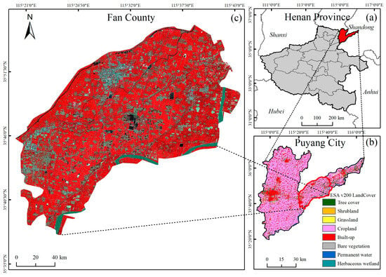
Figure 1.
Overview of the study area. (a) Locations of Puyang city in Henan province, China; (b) land cover of Puyang city (data from ESA (v200)); (c) Fan County with a false-color image of GF-2.
2.2. Data Sources and Pre-Processing
In this study, Landsat 8 OLI multi-spectral images were used for SWIR downscaling. We downloaded Landsat 8 cloud-free images of Fan County in 2023 from Google Earth Engine (GEE) and synthesized them into a single image with the median method, which reduced the influence of extreme values. GEE is a cloud-based geospatial data storage and processing platform that provides pre-processed Landsat series images with atmospheric and radiometric calibrations [50].
The GF-2 multi-spectral images were used for ASI calculation and built-up land extraction, which were acquired from the China Resource Satellite Application Center (https://data.cresda.cn) (accessed on 3 August 2023). Launched on 19 August 2014, the GF-2 satellite is a Chinese civilian high-resolution optical satellite in China and is equipped with both a panchromatic sensor and a multispectral sensor. These images were pre-processed (radiometric calibration, atmospheric correction, geometric correction), mosaicked, and clipped with ENVI 5.3 and ERDAS 2015. The detailed information on the images is listed in Table 1.

Table 1.
The wavelengths, spatial resolutions, and acquisition time of the GF-2 and Landsat-8 images.
In built-up land extraction research [35,36,37], water bodies are often seen as noise or background information that is usually removed. Fan County is located in the downstream beach area of the Yellow River, which contains part of the Yellow River, fishponds, ditches, etc. In this study, we masked the water bodies of more than 100 m2 using the remote sensing index and visual interpretation.
2.3. Methodology
The methodology for this research is shown in the flowchart (Figure 2). Firstly, NDVI and NDWI for downscaling model buildings were calculated on Landsat-8 (30 m) and GF-2 (4 m), respectively. Secondly, a high resolution of 4 m SWIR bands were obtained by downscaling skills through the random forest (RF) method. Thirdly, the SWIR bands (4 m) and the original visible and NIR bands of GF-2 were applied to the calculation of ASI (referred to as to distinguish it from the original index). Additionally, we designed a new index named red roof index (RRI) for rural house extraction, which is explained in detail in Section 2.3.3. Finally, the optimal thresholds were selected for and RRI to extract both urban and rural built-up land. Overall built-up areas were obtained as the union of the two results followed by accuracy validation.
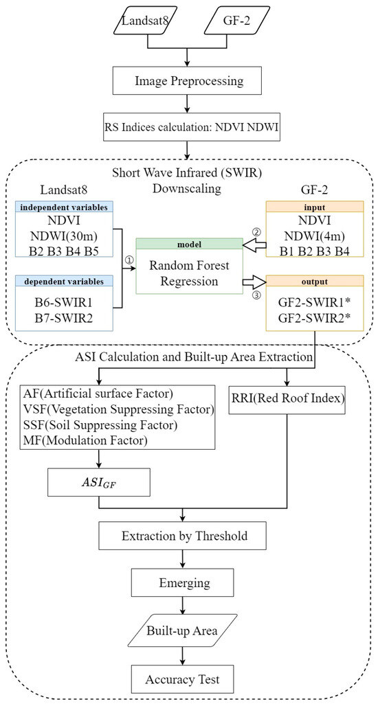
Figure 2.
The flowchart of the methodology.
2.3.1. Downscaling of SWIR Based on RF Regression
We used well-established downscaling methods for TIR bands and land surface temperature (LST) to generate the SWIR bands on the GF-2 image. The foundation of downscaling lies in the correlations between coarse-resolution LST and ancillary biophysical parameters that can be applied at a finer spatial resolution [51]. Original band reflectance, remote sensing indices, topographic factors, and land cover data are commonly employed as predictors in the regression process [52]. Here, we used RF regression to downscale SWIR. Random forest regression is a commonly used machine learning algorithm using bagging techniques, which combines the outputs of multiple decision trees to obtain a single result. The technique helps reduce variance and improve accuracy by combining the predictions from several decision trees.
Medium-resolution satellites equipped with SWIR include the Landsat and Sentinel. Since the spatial resolution of SWIR of Sentinel-2 (20 m) is inconsistent with visible and NIR bands (10 m), the Landsat-8 OLI imagery was chosen as the training data for the RF regression. Subsequently, VNIR bands (B2–B4), NDVI (Normalized Difference Vegetation Index, Equation (2)) and NDWI (Normalized Difference Water Index, Equation (3)) with a resolution of 30 m were designated as independent variables. Simultaneously, SWIR1 (B6) and SWIR2 (B7) were set as dependent variables to establish RF models M1 and M2. Finally, high-resolution NDVI, NDWI, and original bands (B1–B4) from GF-2 were fed into M1 and M2 to derive two SWIR bands (GF-2 SWIR1*, GF-2 SWIR2*) with a resolution of 4 m. The two downscaled SWIR bands can be represented as follows:
where Blue, Green, Red, and NIR are VNIR bands of GF-2 images; NDVI and NDWI are indices derived from GF-2; and f is a non-linear linking model. Regression models were built independently for the two SWIR bands.
where , and are the surface reflectance of the red, green, and NIR bands, respectively.
2.3.2. Artificial Surface Index (ASI)
ASI is a second-level index (Equation (4)), which is composed of the Artificial Surface Factor (AF, Equation (5)), Vegetation Suppressing Factor (VSF, Equation (6)), Soil Suppressing Factor (SSF, Equation (8)), and Modulation Factor (MF, Equation (12)).
The values of ASIGF were normalized to the range of [0, 1] with the min-max normalization function based on the entire image.
where AF is the Artificial Surface Factor, highlighting the spectral characteristics of built-up land, and and are the surface reflectance of the NIR and blue bands. AF highlights the spectral characteristics of built-up land.
where VSF is the Vegetation Suppressing Factor, calculated by two vegetation indices, NDVI (Equation (2)) and MSAVI (Equation (7)), and and are the surface reflectance of the NIR and red bands.
where SSF is the Soil Suppressing Factor, calculated by two bare soil indices (EMBI, Equation (9); MBI, Equation (10)) and the water index (MNDWI, Equation (11)). , , are the surface reflectance of the SWIR1, SWIR2, NIR, and green bands, respectively.
where MF is the Modulation Factor, which is designed to enhance built-up land and suppress bare soil/vegetation, and , are the surface reflectance of the blue, green, NIR, and SWIR bands, respectively.
2.3.3. Red Roof Index (RRI)
In this study, we designed RRI to identify rural buildings precisely. In our study area, most of the rural buildings are made of brick or stone, the roofs of which appear as red colors on the images. Through analysis of the spectral reflectance curve of red roof buildings and in GF-2 (Figure 3), we observed that the reflectance curves of the red roof buildings and the bare soil are similar. However, the spectral curve of red roof buildings from the blue band to red band obviously exhibited a concave shape, while that of bare soil was nearly convex or flat. This phenomenon could be described as the relationship between and twice of , which inspired the design of RRI. In theory, the value of RRI for red roof buildings was positive, while that for bare soil was negative.
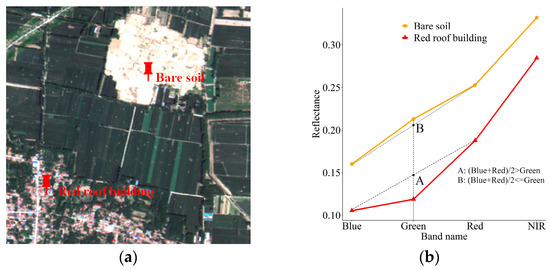
Figure 3.
The sample points (a) and spectral reflectance (b) of red roof buildings and bare soil.
The threshold segmentation method was used to extract the built-up land. The optimal thresholds were determined by representative samples and visual interpretation. We sampled five land cover types, including forest, farmland, urban built-up land, rural built-up land, and bare land, to determine the threshold for ASIGF. Bare soil with different humidity and vegetation covers as well as rural built-up land points were selected to determine the threshold for RRI.
2.3.4. Other Indices for Built-Up Area Extraction
Other five commonly used built-up land indices were calculated to compare with the method we proposed, including NDBI (Equation (14)), BCI (Equation (15)), PISI (Equation (16)), BLFEI (Equation (17)), and UI (Equation (18)).
where , , and are the normalized result of the first three components (brightness, greenness, and humidity) of the tasseled cap (TC) transformation of the GF-2 image. The TC parameters of the IKONOS satellite are commonly used on GF-2 [46] due to the absence of TC parameters for GF-2 and the similarity in wavebands between the two satellites.
2.3.5. Evaluation of SWIR Downscaling
In this study, two image quality metrics were employed to evaluate downscaled SWIR bands, namely contrast (CON) and information entropy (H):
where is the gray level and is the probability of the gray level of on the image. Prior to computing these two metrics, it is necessary to stretch the image to the range of [0, 255].
Additionally, the Pearson correlation coefficient (R) was utilized to quantify the information similarity between the low- and high-resolution SWIR images. The range of R is [−1, 1]. Two variables are positively correlated when R > 0 and vice versa. The larger the absolute value, the stronger the correlation. Furthermore, before calculating the Pearson correlation coefficient, the downscaled SWIR (4 m) bands were aggregated to 30 m by taking the spatial average of neighbor pixels to align with SWIR bands of Landsat-8 in resolution.
2.3.6. Accuracy Assessment of the Built-Up Area Extraction
Separability tests and histogram comparisons were performed for indices to determine the separability between built-up and non-built-up pixels [35,36]. The separability metrics include the Jeffries–Matusita distance (JMD) [53], the Transformed Divergence (TD) [54], and the Spectral Discrimination Index (SDI) [55]. The ranges of JMD and TD are (0, √2] and (0, 2], respectively, with no limit for SDI. Larger values indicate a higher degree of separability.
The confusion matrix is the most commonly used method for accuracy testing in remote sensing research. It is a standard method that includes the indicators overall accuracy (OA), Kappa coefficient (Kappa), commission error (CE), omission error (OE), mapper accuracy (MA), and user accuracy (UA).
To ensure that most of the validation points are from real built-up areas, we randomly chose 3/4 of the validation points from the built-up area we extracted, and the remaining 1/4 points were randomly chosen from a non-built-up area.
3. Results
3.1. Analysis of SWIR Downscaling
A total of 50,000 random points were generated for the entirety of Fan County, which were divided into the training set and testing set at a ratio of 4:1. The two main parameters for the random forest (RF) were the max number of trees (N) and max depth of trees (D). The 10-fold cross-validation technique was used to determine the optimal parameters. This process was conducted in ArcGIS Pro 3.1 automatically. In our study, N was 50 and D was 27. The coefficient of determination (R-squared) was also computed as an estimate of the goodness of fit. As Table 2 shows, the R-squared of two SWIR bands on both the training set and testing set were better than 85%, which indicates the good performance of our regression models.

Table 2.
R-squared of random forest regression model.
Six typical regions of three land cover types, towns, allocation communities, and villages, were selected to demonstrate and evaluate the SWIR downscaling from Landsat-8 to GF-2 in detail. It is evident that the spatial details are more distinctly visible in the downscaled SWIR band (Figure 4).
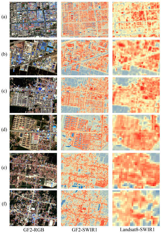
Figure 4.
Comparisons of downscaled and original SWIR1 bands. RGB means the red, green, and blue channels for image displaying. (a,b) towns; (c,d) allocation communities; (e,f) villages.
In the urban area (Figure 4a) and the factories (Figure 4b) in Fan County, the downscaled SWIR band images distinctly outline individual buildings. Additionally, the bare soil shows relatively high reflectance in SWIR bands on both Landsat-8 and GF-2, particularly in areas with sparse vegetation cover and high soil water content.
In the allocation communities (Figure 4c,d), the buildings exhibit regular shapes and roofs in dark colors. This characteristic is manifested in the SWIR band as lower reflectance, in contrast to the common blue or white roofs in other regions.
In the rural areas (Figure 4e,f), the internal structure and layout framework of the traditional rural settlements are better presented in the high-resolution SWIR images. However, the reflectance difference of built-up/non-built-up land in the rural area is lower than that in the urban area, posing potential challenges in the extraction of rural built-up areas.
To quantitatively evaluate the SWIR downscaling, the contrast and information entropy were computed for both low- and high-resolution images in the regions mentioned above. As shown in Table 3, the contrast of the downscaled SWIR bands is significantly improved, with nearly no difference in terms of information in comparison to the SWIR bands of the Landsat-8 images. This confirms that the downscaling method effectively enriches the spatial details of images while preserving the information the bands contain.

Table 3.
The contrast and information entropy of downscaled and original SWIR images sampled from the six typical regions.
Additionally, to verify the information similarity between the original and downscaled bands, the Pearson correlation analysis was performed on the values of 15,000 random points on the SWIR bands. Figure 5 shows that there is a strong correlation (R = 0.75) between coarse and aggregated fine resolution SWIR1 and SWIR2 images under the 95% confidence level.
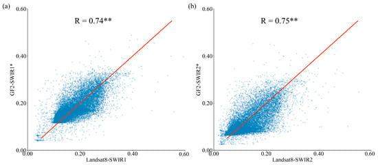
Figure 5.
Correlation coefficient between downscaled and original SWIR1 (a) and SWIR2 (b) bands. (** indicates significant at 95% confidence level).
By adopting the generally used and highly efficient RF regression method, our results not only excelled in preserving image information of the original bands but also yielded remarkable improvements in terms of spatial resolution. Consequently, the SWIR bands generated through the downscaling technique were highly reliable for calculating remote sensing indices in high-resolution images.
3.2. Built-Up Land Extraction by Threshold Segmentation
The built-up land extraction was conducted by indices calculation and threshold segmentation. In this section, we discuss the optical threshold settings for ASI and RRI first. Then, the two indices are combined together to map the built-up area in Fan County. The accuracy assessment is conducted for the whole study area based on the extraction results from our approach.
3.2.1. Optical Thresholds for ASI and RRI
To determine the optical threshold for , we selected three categories of samples—urban built-up land, rural built-up land, and non-built-up land, with 2000 points for each type. The histogram of these samples is shown in Figure 6a. During the process of threshold setting for , we observed a more effective distinction between urban built-up areas and non-built-up areas compared to rural built-up land on , as the latter is more prone to confusion with bare land. As shown in Figure 6, the threshold of being under 0.8 (Figure 6c) led to serious confusion between rural buildings and bare soil. When the threshold for was set to greater than 0.8 (Figure 6e), large quantities of buildings with high-reflectance roofs were omitted. Therefore, the optical segmentation threshold was 0.8 to both suppress bare soil and maintain urban buildings. Furthermore, the gradual increase in the threshold led to a notable increase in the omission of rural buildings with red roofs.
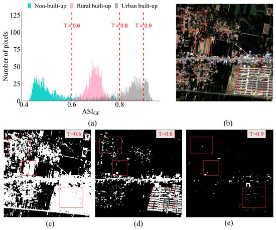
Figure 6.
Threshold segmentation results of with different thresholds. (a) Histogram of , where “T” means threshold; (b) RGB image; (c–e) segmentation results with thresholds set to 0.6, 0.8, and 0.9.
To further validate the performance of to separate built-up land from non-built-up land, a comparison and analysis were conducted on five commonly used indices related to built-up area extraction: UI, BLFEI, NDBI, BCI, and PISI. As the histogram (Figure 7) and separability indices (Table 4) show, exhibited the best performance in distinguishing urban built-up land from non-built-up land. In terms of distinguishing rural built-up land from non-built-up land, outperformed UI and BLFEI, while it was slightly inferior compared to NDBI, BCI, and PISI. Consequently, performed well for urban built-up land extraction and had a strong suppression of bare soil, but its ability to distinguish rural buildings from bare ground was inadequate.
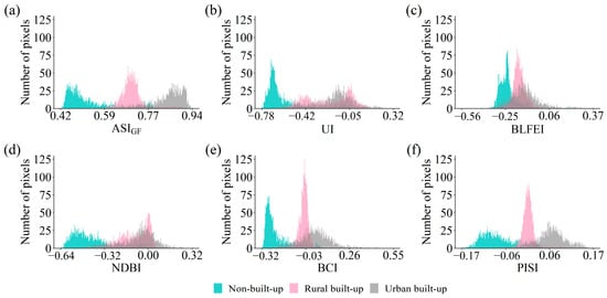
Figure 7.
The histogram of non-built-up areas, rural built-up areas, and urban built-up areas for (a), UI (b), BLFEI (c), NDBI (d), BCI (e), and PISI (f).

Table 4.
Separability between non-built-up areas and built-up areas for and five other indices.
The value range of RRI was not fixed according to its principle. For Fan County, the minimum and maximum values of RRI were −0.28 and 0.43. The threshold for RRI was visually judged to 0.01 to extract rural buildings omitted by .
To further illustrate the important complementary role of RRI, we selected 200 random points to conduct an accuracy test, among which 150 points were rural buildings while the remaining 50 points belonged to non-built-up land. As shown in Table 5, RRI acquired high accuracy when extracting rural built-up land. The complementary nature of RRI increased the overall accuracy and reduced the omission of rural buildings. The result of was not satisfactory, especially the high omission errors. This is because most of the rural built-up land was classified as background information given the threshold of 0.8.

Table 5.
Confusion matrix and accuracy assessment of rural built-up area extraction results using and RRI.
3.2.2. Built-Up Land Extraction Results
The final result for the built-up area in Fan County was the union of the extraction results of and RRI (Figure 8). This process not only eliminated the bare land but also extracted the red roof rural buildings omitted by . Most of the houses in the rural settlements have red roofs, which could be extracted by the RRI we designed. The rest of the buildings (such as factories) have blue or white roofs, which have high reflectance and can be extracted by . Therefore, the best extraction results can be achieved by combining the two indices.
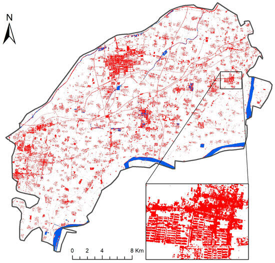
Figure 8.
Built-up area extraction results in Fan County (red color indicates the built-up land, blue indicates the water body).
In the urban area (Figure 9a) and clustered factories regions (Figure 9b) in Fan County, the prominent features include asphalt roads and high-albedo buildings with white or blue roofs. On the other hand, the allocation communities (Figure 9c,d) are new rural communities situated within the township area. Rural settlements (Figure 9e,f) are characterized by fine country roads and dense rural houses built with a mixture of brick and earth, featuring red or orange roofs, along with scattered concrete factories or stores.
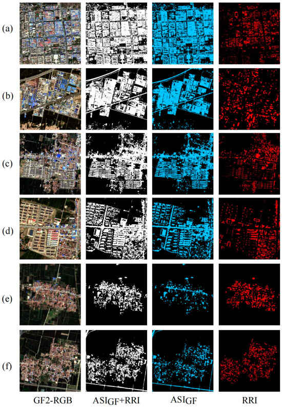
Figure 9.
Built-up area extraction results of and RRI. RGB means the red, green, and blue channels for image displaying. (a,b) towns; (c,d) allocation communities; (e,f) villages.
3.2.3. Accuracy Assessment
To validate the accuracy of the extraction results, 600 sample points were randomly selected from the entirety of Fan County, and the real land use types of these samples were obtained by visual interpretation on images with higher resolution. The confusion matrix and accuracy metrics (Table 6) revealed that the extraction of built-up land by the combination of and RRI is effective, with an overall accuracy of more than 90% and a Kappa coefficient of 0.83. The misclassified pixels were mainly from fallow land with high humidity and surfaces covered with sparse vegetation.

Table 6.
Confusion matrix and accuracy assessment of built-up area extraction results using the combination of and RRI.
In addition, by analyzing the histogram of (Figure 6), it can be found that to effectively distinguish built-up land from non-built-up land, the optimal threshold falls in the range of rural built-up land, which is an important reason for the inevitable misclassification of rural construction land.
3.3. Comparison with Five Other Index-Based Methods
To verify the effectiveness of RRI in addressing the confusion between rural built-up land and bare soil, we selected 2000 sample points from bare soil in the images. Histograms (Figure 10) and a separability test (Table 7) demonstrated that, compared with other indices, RRI excels in distinguishing rural built-up land from bare land. It exhibits the best performance with a JMD close to the maximum value () and the TD value close to 2, indicating a strong ability to distinguish the two land use types.
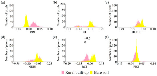
Figure 10.
The histograms of rural built-up areas and bare land for RRI (a), UI (b), BLFEI (c), NDBI (d), BCI (e), and PISI (f).

Table 7.
Separability between rural built-up areas and bare land for five other indices and RRI.
Based on the comprehensive analysis above, a further comparison of + RRI with the other three indices (NDBI, BCI, and PISI) that excel in distinguishing built-up land from non-built-up land was conducted. The extraction result comparisons (Figure 11) and accuracy validation (Table 8) demonstrated that the combination of and RRI works most effectively in the extraction of built-up land.
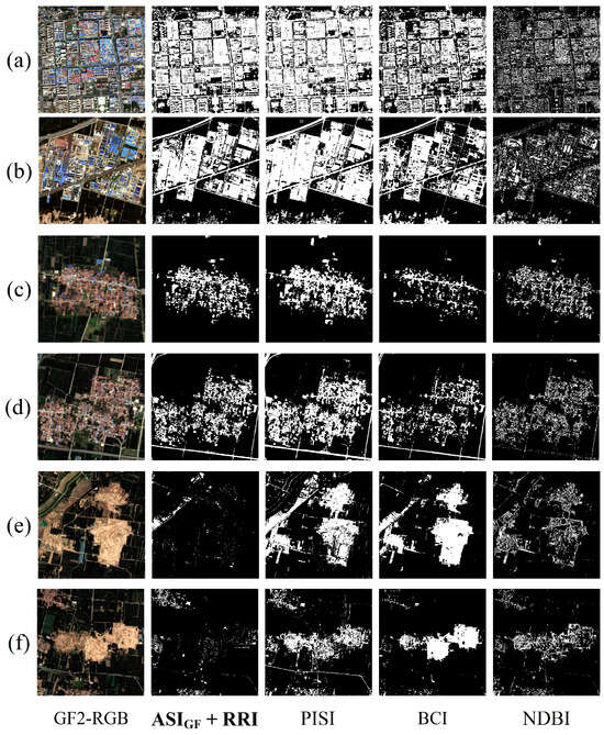
Figure 11.
The extraction results using + RRI, PISI, BCI, and NDBI. (a,b) towns; (c,d) allocation communities; (e,f) bare land.

Table 8.
Accuracy assessment of three other methodologies and the combination of and RRI.
In the extraction of urban built-up land (Figure 11a,b), + RRI, NDBI, and BCI exhibited superior performance, with no significant difference among the three methods. In the extraction of rural settlements (Figure 11c,d), + RRI demonstrated distinct advantages over PISI and NDBI. + RRI accurately extracts rural houses and effectively suppresses bare land in rural settlements. NDBI, on the other hand, suppresses both rural houses and bare soil, resulting in relatively low extraction accuracy. Regarding the bare soil shown in Figure 11e,f (i.e., leveled bare soil after a house demolition with low water content), + RRI effectively removes it, further confirming its superiority in built-up land extraction.
In conclusion, the combination of and RRI proved to be effective for extracting built-up land, particularly in rural areas, and suppressing bare land. This finding presents innovative ideas and methods for rural built-up land extraction, which are expected to benefit future research.
4. Discussion
4.1. The Application of the SWIR Downscaling Technique in High-Resolution Built-Up Land Extraction
In the field of remote sensing, many studies have adopted downscaling methods for TIR bands, but not in SWIR. This study successfully generated two SWIR bands of 4 m resolution using the RF regression method. Our method enables the effective application of built-up area indices (e.g., ASI, NDBI, etc.) that rely on SWIR information from high-resolution images that lack these two bands originally. This allows for finer extraction of built-up land.
From a technical perspective, the downscaling method preserves the information of the original band while significantly enhancing its spatial resolution. This technique is an image fusion method [56] that relies on the correlation between the reflectance of the target band and predictors, like other bands or remote sensing indices within the same region and at the same time. However, this method has limitations. It requires that the high- and low-resolution images used for modeling are temporally similar; otherwise, the temporal variations in the spectral characteristics of features may introduce errors. Additionally, the method is limited to improving the spatial resolution of the bands and adding missing bands to the high-resolution image rather than enhancing its temporal resolution. The enhancement of the temporal resolution by integrating satellite data with different revisiting periods contributes to continuous monitoring of land use change. There are still some challenges during the process of image fusion, including image registering, noise removal, and increased computational demands [57,58,59]. The SWIR downscaling method we proposed is able to enhance the spatial resolution of SWIR bands, providing additional bands for high-resolution images. The temporal resolution enhancement has been little emphasized in our study.
The application of spectral indices on high-resolution built-up land extraction has been limited due to the incapability of most high-resolution sensors to detect SWIR band information, which is crucial for distinguishing built-up land from other land use types. Indices designed for high-resolution images primarily rely on visible and NIR bands, posing limitations in fully leveraging the spectral characteristics of built-up land. In this study, the SWIR bands were successfully integrated into the high-resolution image through downscaling techniques. This expands the application of various built-up land indices on high-resolution images.
4.2. RRI Improves the Separability between Rural Buildings and Bare Land
Significant progress has been made in the research on built-up areas or building extraction in large and medium-sized cities. However, in economically underdeveloped and agriculture-oriented counties, especially in floodplain regions like Fan County, there is still insufficient research. These counties exhibit a low urbanization rate, limited urban built-up land area, and scattered distribution of rural construction land as the main characteristics of land use. The majority of rural houses in these areas are brick structures with red roofs, sharing certain spectral characteristics with bare soil. This similarity poses challenges to the extraction of rural built-up land.
Indices related to built-up area currently in use are primarily designed to differentiate between urban built-up areas and other land types, including bare land. However, the consideration of rural housing characteristics is not yet sufficient, leading to a weak distinction between rural construction land and bare land. We designed RRI to address this issue and validated its effectiveness through three separability indices. RRI alone may not be ideal for urban built-up land extraction, but its combination with other indices can significantly enhance the accuracy of built-up land extraction in rural areas.
This paper demonstrates the effectiveness of the + RRI method in extracting built-up land in rural areas of the central China plain. The findings offer a novel approach for rural construction land extraction with potential significance for future research and application. Given the complexity of rural built-up land, along with potential errors caused by elevation, subsequent research should involve built-up land extraction experiments in diverse rural settings (e.g., mountainous areas) to test the generalizability of the proposed index.
5. Conclusions
This paper introduced a rapid extraction method for built-up land in rural areas on high-resolution remote sensing images lacking SWIR bands. The methodology was applied and examined in Fan County, Henan Province. Two 4 m resolution SWIR bands were generated through the downscaling method by RF regression with predictors like NDVI and NDWI. The high-resolution SWIR bands, along with the original bands of the GF-2 images, were then applied to calculate , which exhibited superior accuracy in urban built-up land extraction. In rural areas, five other indices (NDBI, BCI, etc.) did not performed well when discriminating rural built-up areas and non-built-up areas. This challenge was effectively addressed by the RRI we proposed in this study. The accuracy assessment demonstrated that, compared with three other commonly used indices, the combination of and RRI achieved the highest performance, with an overall accuracy of 93.33% and Kappa of 83.12%. In summary, our methodology has the potential and advantage of efficient extraction of built-up land in rural areas on HR images without SWIR bands.
There are still some limitations to our approach. Firstly, the determination of thresholds for ASI and RRI requires experiments according to different areas. In this study, the threshold of ASI was set to 0.8 with the aim of excluding bare soil. The threshold setting for RRI was intended to extract red roof buildings omitted by ASI. Secondly, further validation will be needed by using the method on other regions. RRI performs well in the extraction of specifically red roof buildings, and further validation will be needed for other types of buildings.
Author Contributions
Conceptualization, W.Z., C.Y. and Y.T.; methodology, W.Z., C.Y., Y.T. and Y.W.; validation, W.Z. and Y.W.; formal analysis, W.Z., C.Y. and Y.T.; investigation, W.Z., Y.W. and C.H.; writing—original draft preparation, W.Z.; writing—review and editing, C.Y. and L.L.; visualization, W.Z. and L.L.; supervision, Y.T.; funding acquisition, C.Y. All authors have read and agreed to the published version of the manuscript.
Funding
This research was funded by Major Project of Chinese High-resolution Earth Observation System, grant number 00-Y30B01-9001-22/23.
Data Availability Statement
The data presented in this study are available on reasonable request from the corresponding author.
Acknowledgments
Special thanks are extended to Huang Huiping (Aerospace Information Research Institute, Chinese Academy of Sciences) for her guidance and encouragement with the experiment and writing.
Conflicts of Interest
The authors declare no conflicts of interest.
References
- Das, T.; Shahfahad; Naikoo, M.W.; Talukdar, S.; Parvez, A.; Rahman, A.; Pal, S.; Asgher, M.S.; Islam, A.R.M.T.; Mosavi, A. Analysing Process and Probability of Built-Up Expansion Using Machine Learning and Fuzzy Logic in English Bazar, West Bengal. Remote Sens. 2022, 14, 2349. [Google Scholar] [CrossRef]
- Gao, X.; Wu, M.; Niu, Z.; Chen, F. Global Identification of Unelectrified Built-Up Areas by Remote Sensing. Remote Sens. 2022, 14, 1941. [Google Scholar] [CrossRef]
- Ruan, L.; He, T.; Xiao, W.; Chen, W.; Lu, D.; Liu, S. Measuring the Coupling of Built-up Land Intensity and Use Efficiency: An Example of the Yangtze River Delta Urban Agglomeration. Sustain. Cities Soc. 2022, 87, 104224. [Google Scholar] [CrossRef]
- Wang, H.; Gong, X.; Wang, B.; Deng, C.; Cao, Q. Urban Development Analysis Using Built-up Area Maps Based on Multiple High-Resolution Satellite Data. Int. J. Appl. Earth Obs. Geoinf. 2021, 103, 102500. [Google Scholar] [CrossRef]
- Chuai, X.; Huang, X.; Lu, Q.; Zhang, M.; Zhao, R.; Lu, J. Spatiotemporal Changes of Built-Up Land Expansion and Carbon Emissions Caused by the Chinese Construction Industry. Environ. Sci. Technol. 2015, 49, 13021–13030. [Google Scholar] [CrossRef]
- Morabito, M.; Crisci, A.; Messeri, A.; Orlandini, S.; Raschi, A.; Maracchi, G.; Munafò, M. The Impact of Built-up Surfaces on Land Surface Temperatures in Italian Urban Areas. Sci. Total Environ. 2016, 551–552, 317–326. [Google Scholar] [CrossRef]
- Wang, J.; Hadjikakou, M.; Bryan, B.A. Consistent, Accurate, High Resolution, Long Time-Series Mapping of Built-up Land in the North China Plain. GIScience Remote Sens. 2021, 58, 982–998. [Google Scholar] [CrossRef]
- Zhang, Y.; Chen, Z.; Cheng, Q.; Zhou, C.; Jiang, P.; Li, M.; Chen, D. Quota Restrictions on Land Use for Decelerating Urban Sprawl of Mega City: A Case Study of Shanghai, China. Sustainability 2016, 8, 968. [Google Scholar] [CrossRef]
- Peres, L.D.F.; Lucena, A.J.D.; Rotunno Filho, O.C.; França, J.R.D.A. The Urban Heat Island in Rio de Janeiro, Brazil, in the Last 30 Years Using Remote Sensing Data. Int. J. Appl. Earth Obs. Geoinf. 2018, 64, 104–116. [Google Scholar] [CrossRef]
- Xu, H.; Xiao, X.; Qin, Y.; Qiao, Z.; Long, S.; Tang, X.; Liu, L. Annual Maps of Built-Up Land in Guangdong from 1991 to 2020 Based on Landsat Images, Phenology, Deep Learning Algorithms, and Google Earth Engine. Remote Sens. 2022, 14, 3562. [Google Scholar] [CrossRef]
- Gong, J.; Liu, C.; Huang, X. Advances in Urban Information Extraction from High-Resolution Remote Sensing Imagery. Sci. China Earth Sci. 2020, 63, 463–475. [Google Scholar] [CrossRef]
- Li, J.; Huang, X.; Tu, L.; Zhang, T.; Wang, L. A Review of Building Detection from Very High Resolution Optical Remote Sensing Images. GIScience Remote Sens. 2022, 59, 1199–1225. [Google Scholar] [CrossRef]
- Bi, Q.; Qin, K.; Zhang, H.; Zhang, Y.; Li, Z.; Xu, K. A Multi-Scale Filtering Building Index for Building Extraction in Very High-Resolution Satellite Imagery. Remote Sens. 2019, 11, 482. [Google Scholar] [CrossRef]
- Shao, Z.; Cheng, T.; Fu, H.; Li, D.; Huang, X. Emerging Issues in Mapping Urban Impervious Surfaces Using High-Resolution Remote Sensing Images. Remote Sens. 2023, 15, 2562. [Google Scholar] [CrossRef]
- Suharyadi, R.; Umarhadi, D.A.; Awanda, D.; Widyatmanti, W. Exploring Built-Up Indices and Machine Learning Regressions for Multi-Temporal Building Density Monitoring Based on Landsat Series. Sensors 2022, 22, 4716. [Google Scholar] [CrossRef] [PubMed]
- Ul Din, S.; Mak, H.W.L. Retrieval of Land-Use/Land Cover Change (LUCC) Maps and Urban Expansion Dynamics of Hyderabad, Pakistan via Landsat Datasets and Support Vector Machine Framework. Remote Sens. 2021, 13, 3337. [Google Scholar] [CrossRef]
- Tikuye, B.G.; Rusnak, M.; Manjunatha, B.R.; Jose, J. Land Use and Land Cover Change Detection Using the Random Forest Approach: The Case of The Upper Blue Nile River Basin, Ethiopia. Glob. Chall. 2023, 7, 2300155. [Google Scholar] [CrossRef]
- Li, S.; Fu, S.; Zheng, D. Rural Built-Up Area Extraction from Remote Sensing Images Using Spectral Residual Methods with Embedded Deep Neural Network. Sustainability 2022, 14, 1272. [Google Scholar] [CrossRef]
- Zheng, J.; Tian, Y.; Yuan, C.; Yin, K.; Zhang, F.; Chen, F.; Chen, Q. MDESNet: Multitask Difference-Enhanced Siamese Network for Building Change Detection in High-Resolution Remote Sensing Images. Remote Sens. 2022, 14, 3775. [Google Scholar] [CrossRef]
- Tan, Y.; Xiong, S.; Li, Y. Automatic Extraction of Built-Up Areas from Panchromatic and Multispectral Remote Sensing Images Using Double-Stream Deep Convolutional Neural Networks. IEEE J. Sel. Top. Appl. Earth Obs. Remote Sens. 2018, 11, 3988–4004. [Google Scholar] [CrossRef]
- Chen, T.-H.K.; Pandey, B.; Seto, K.C. Detecting Subpixel Human Settlements in Mountains Using Deep Learning: A Case of the Hindu Kush Himalaya 1990–2020. Remote Sens. Environ. 2023, 294, 113625. [Google Scholar] [CrossRef]
- Ichsan Ali, M.; Hafid Hasim, A.H.H.; Raiz Abidin, M. Monitoring the Built-up Area Transformation Using Urban Index and Normalized Difference Built-up Index Analysis. Int. J. Eng. 2019, 32, 647–653. [Google Scholar] [CrossRef]
- Bouzekri, S.; Lasbet, A.A.; Lachehab, A. A New Spectral Index for Extraction of Built-Up Area Using Landsat-8 Data. J. Indian Soc. Remote Sens. 2015, 43, 867–873. [Google Scholar] [CrossRef]
- Huang, X.; Zhang, L.; Zhu, T. Building Change Detection from Multitemporal High-Resolution Remotely Sensed Images Based on a Morphological Building Index. IEEE J. Sel. Top. Appl. Earth Obs. Remote Sens. 2014, 7, 105–115. [Google Scholar] [CrossRef]
- Shao, Z.; Tian, Y.; Shen, X. BASI: A New Index to Extract Built-up Areas from High-Resolution Remote Sensing Images by Visual Attention Model. Remote Sens. Lett. 2014, 5, 305–314. [Google Scholar] [CrossRef]
- Xu, H. Analysis of Impervious Surface and Its Impact on Urban Heat Environment Using the Normalized Difference Impervious Surface Index (NDISI). Photogramm. Eng. Remote Sens. 2010, 76, 557–565. [Google Scholar] [CrossRef]
- As-syakur, A.R.; Adnyana, I.W.S.; Arthana, I.W.; Nuarsa, I.W. Enhanced Built-Up and Bareness Index (EBBI) for Mapping Built-Up and Bare Land in an Urban Area. Remote Sens. 2012, 4, 2957–2970. [Google Scholar] [CrossRef]
- Zhang, P.; Sun, Q.; Liu, M.; Li, J.; Sun, D. A Strategy of Rapid Extraction of Built-Up Area Using Multi-Seasonal Landsat-8 Thermal Infrared Band 10 Images. Remote Sens. 2017, 9, 1126. [Google Scholar] [CrossRef]
- Zha, Y.; Gao, J.; Ni, S. Use of Normalized Difference Built-up Index in Automatically Mapping Urban Areas from TM Imagery. Int. J. Remote Sens. 2003, 24, 583–594. [Google Scholar] [CrossRef]
- Xu, H. A New Index for Delineating Built-up Land Features in Satellite Imagery. Int. J. Remote Sens. 2008, 29, 4269–4276. [Google Scholar] [CrossRef]
- Tang, Y.; Liu, Z.J.; Yang, S.W. Mapping Urban Built-up Land in Northwest China Based on Three-index Synthetic Remote Sensing Imagery. J. Geo-Inf. Sci. 2019, 21, 1455–1466. [Google Scholar]
- Li, F.G.; Li, E.Z.; Samat, A.; Zhang, L.P.; Liu, W.; Hu, J.S. Estimation of large-scale impervious surface percentage by fusion of multi-source time series remote sensing data. J. Remote Sens. 2020, 24, 243–1254. [Google Scholar] [CrossRef]
- Xu, R.; Liu, J.; Xu, J. Extraction of High-Precision Urban Impervious Surfaces from Sentinel-2 Multispectral Imagery via Modified Linear Spectral Mixture Analysis. Sensors 2018, 18, 2873. [Google Scholar] [CrossRef]
- Bouhennache, R.; Bouden, T.; Taleb-Ahmed, A.; Cheddad, A. A New Spectral Index for the Extraction of Built-up Land Features from Landsat 8 Satellite Imagery. Geocarto Int. 2019, 34, 1531–1551. [Google Scholar] [CrossRef]
- Zhao, Y.; Zhu, Z. ASI: An Artificial Surface Index for Landsat 8 Imagery. Int. J. Appl. Earth Obs. Geoinf. 2022, 107, 102703. [Google Scholar] [CrossRef]
- Deng, C.; Wu, C. BCI: A Biophysical Composition Index for Remote Sensing of Urban Environments. Remote Sens. Environ. 2012, 127, 247–259. [Google Scholar] [CrossRef]
- Tian, Y.; Chen, H.; Song, Q.; Zheng, K. A Novel Index for Impervious Surface Area Mapping: Development and Validation. Remote Sens. 2018, 10, 1521. [Google Scholar] [CrossRef]
- Yang, W.; Zhang, Y.; Yin, X. Construction of Ratio Build-up Index for GF-1 Image. Remote Sens. Land Resour. 2016, 28, 35–42. [Google Scholar]
- Zhang, Y.; Chen, Y.; Xue, Y.; Lin, J. Construction of Urban Built-up Index Oriented to GF-1 WFV Image. Geomat. Spat. Inf. Technol. 2019, 42, 84–88. [Google Scholar]
- Bai, Y.; He, G.; Wang, G.; Yang, G. WE-NDBI-A New Index for Mapping Urban Built-up Areas from GF-1 WFV Images. Remote Sens. Lett. 2020, 11, 407–415. [Google Scholar] [CrossRef]
- Zhang, L.; Peng, M.; Sun, X.; Cen, Y.; Tong, Q. Progress and bibliometric analysis of remote sensing data fusion methods (1992—2018). J. Remote Sens. 2019, 23, 603–619. [Google Scholar] [CrossRef]
- Stathopoulou, M.; Cartalis, C. Downscaling AVHRR Land Surface Temperatures for Improved Surface Urban Heat Island Intensity Estimation. Remote Sens. Environ. 2009, 113, 2592–2605. [Google Scholar] [CrossRef]
- Njuki, S.M.; Mannaerts, C.M.; Su, Z. An Improved Approach for Downscaling Coarse-Resolution Thermal Data by Minimizing the Spatial Averaging Biases in Random Forest. Remote Sens. 2020, 12, 3507. [Google Scholar] [CrossRef]
- Zhao, W.; Duan, S.-B.; Li, A.; Yin, G. A Practical Method for Reducing Terrain Effect on Land Surface Temperature Using Random Forest Regression. Remote Sens. Environ. 2019, 221, 635–649. [Google Scholar] [CrossRef]
- Hutengs, C.; Vohland, M. Downscaling Land Surface Temperatures at Regional Scales with Random Forest Regression. Remote Sens. Environ. 2016, 178, 127–141. [Google Scholar] [CrossRef]
- Xu, S. Research on Spatial Downscaling Method of Land Surface Temperature and Its Application. Ph.D. Thesis, Aerospace Information Research Institute, Chinese Academy of Sciences, Beijing, China, 2021. [Google Scholar]
- Li, S.; Tang, H.; Yang, X. Spectral Residual Model for Rural Residential Region Extraction from GF-1 Satellite Images. Math. Probl. Eng. 2016, 1–13. [Google Scholar] [CrossRef]
- Wang, Z.; Li, S.; Zhu, Z. Rural Building Extraction Based on Joint U-Net and the Generalized Chinese Restaurant Franchise from Remote Sensing Images. Sustainability 2023, 15, 4685. [Google Scholar] [CrossRef]
- Zheng, X.; Wu, B.; Weston, M.; Zhang, J.; Gan, M.; Zhu, J.; Deng, J.; Wang, K.; Teng, L. Rural Settlement Subdivision by Using Landscape Metrics as Spatial Contextual Information. Remote Sens. 2017, 9, 486. [Google Scholar] [CrossRef]
- Yang, L.; Driscol, J.; Sarigai, S.; Wu, Q.; Chen, H.; Lippitt, C.D. Google Earth Engine and Artificial Intelligence (AI): A Comprehensive Review. Remote Sens. 2022, 14, 3253. [Google Scholar] [CrossRef]
- Pan, X.; Zhu, X.; Yang, Y.; Cao, C.; Zhang, X.; Shan, L. Applicability of Downscaling Land Surface Temperature by Using Normalized Difference Sand Index. Sci. Rep. 2018, 8, 9530. [Google Scholar] [CrossRef] [PubMed]
- Yang, X.; Meng, F.; Fu, P.; Zhang, J.; Liu, Y. Instability of Remote Sensing Ecological Index and Its Optimisation for Time Frequency and Scale. Ecol. Inform. 2022, 72, 101870. [Google Scholar] [CrossRef]
- Swain, P.H.; Davis, S.M. Remote Sensing: The Quantitative Approach. IEEE Trans. Pattern Anal. Mach. Intell. 1981, 3, 713–714. [Google Scholar] [CrossRef]
- Chang, C.-I. New Hyperspectral Discrimination Measure for Spectral Characterization. Opt. Eng. 2004, 43, 1777. [Google Scholar] [CrossRef]
- Kaufman, Y.J.; Remer, L.A. Detection of Forests Using Mid-IR Reflectance: An Application for Aerosol Studies. IEEE Trans. Geosci. Remote Sens. 1994, 32, 672–683. [Google Scholar] [CrossRef]
- Jing, Y.; Shen, H.; Li, X. Spatial Downscaling of Remote Sensing Parameters from the Perspective of Data Fusion. Geomat. Inf. Sci. Wuhan Univ. 2024, 49, 175–189. Available online: https://kns.cnki.net/kcms/detail/42.1676.TN.20230801.1715.001.html (accessed on 3 August 2023).
- Li, S.; Li, C.; Kang, X. Development status and future prospects of multi-source remote sensing image fusion. Natl. Remote Sens. Bull. 2021, 25, 148–166. [Google Scholar] [CrossRef]
- Ghassemian, H. A Review of Remote Sensing Image Fusion Methods. Inf. Fusion 2016, 32, 75–89. [Google Scholar] [CrossRef]
- Karim, S.; Tong, G.; Li, J.; Qadir, A.; Farooq, U.; Yu, Y. Current Advances and Future Perspectives of Image Fusion: A Comprehensive Review. Inf. Fusion 2023, 90, 185–217. [Google Scholar] [CrossRef]
Disclaimer/Publisher’s Note: The statements, opinions and data contained in all publications are solely those of the individual author(s) and contributor(s) and not of MDPI and/or the editor(s). MDPI and/or the editor(s) disclaim responsibility for any injury to people or property resulting from any ideas, methods, instructions or products referred to in the content. |
© 2024 by the authors. Licensee MDPI, Basel, Switzerland. This article is an open access article distributed under the terms and conditions of the Creative Commons Attribution (CC BY) license (https://creativecommons.org/licenses/by/4.0/).