Deep Learning-Based Landslide Recognition Incorporating Deformation Characteristics

Abstract

Landslide disasters pose a significant threat, with their highly destructive nature underscoring the critical importance of timely and accurate recognition for effective early warning systems and emergency response efforts. In recent years, substantial advancements have been made in the realm of landslide recognition (LR) based on remote sensing data, leveraging deep learning techniques. However, the intricate and varied environments in which landslides occur often present challenges in detecting subtle changes, especially when relying solely on optical remote sensing images. InSAR (Interferometric Synthetic Aperture Radar) technology emerges as a valuable tool for LR, providing more detailed ground deformation data and enhancing the theoretical foundation. To harness the slow deformation characteristics of landslides, we developed the FCADenseNet model. This model is designed to learn features and patterns within ground deformation data, with a specific focus on improving LR. A noteworthy aspect of our model is the integration of an attention mechanism, which considers various monitoring factors. This holistic approach enables the comprehensive detection of landslide disasters across entire watersheds, providing valuable information on landslide hazards. Our experimental results demonstrate the effectiveness of the FCADenseNet model, with an F1-score of 0.7611, which is 9.53% higher than that of FC_DenseNet. This study substantiates the feasibility and efficacy of combining InSAR with deep learning methods for LR. The insights gained from this research contribute to the advancement of regional landslide geological hazard monitoring, identification, and prevention strategies.

1. Introduction

Landslide is a geological disaster characterized by sudden, rapid, and irreversible movement. Typically occurring in terrain such as mountain slopes, river banks, or geotechnical slopes, landslides involve the downward sliding of soil and rocks due to the influence of gravity or other factors. Given China’s mountainous landscape and distinctive energy gradient, coupled with human engineering activities, the country is prone to frequent geological disasters, including landslides [1]. In 2022, China experienced a total of 5659 geological disasters, with landslide geological disasters accounting for a significant 70%, totaling 3919 incidents. These events resulted in substantial life and economic losses [2]. Landslides, influenced by external factors such as intense or sustained precipitation, earthquakes, and human activities, as well as internal factors such as loose rock and soil structures and geological structural damage, are marked by their strong destructiveness and high risk [3]. Landslides pose a significant threat to the lives of society and individuals. Such disasters often lead to road destruction and disruptions in traffic, hindering investigators’ swift access to the disaster site for immediate assessments. Therefore, the rapid and timely acquisition of landslide disaster information and the establishment of landslide inventory maps are crucial for effective subsequent responses to landslide risks [4,5].

In recent years, extensive studies have focused on landslide recognition (LR). The initial methods for LR involved manual visual interpretation. This method usually requires interpreters to have rich experiences, and is subjectively influenced and time-consuming, making it difficult to meet the needs of processing a large amount of information [6]. Subsequently, computer-aided methods were introduced. However, due to the increasingly complex spectral features, the classification efficacy remained unsatisfactory. As computer algorithms continued to evolve, researchers progressively integrated mainstream machine learning algorithms into LR, encompassing artificial neural networks [7], support vector machines [8], random forests [9], and decision trees [10]. Despite enhancing performance, these algorithms encountered difficulties in processing extensive remote sensing (RS) data and extracting deep-dimensional information from various image datasets. Deep learning algorithms (DLAs) can automatically extract meaningful feature representations from images [11]. Through the construction of deep neural networks, DLAs can acquire sophisticated and abstract features from raw data. Research on LR based on DLAs can be broadly categorized into three categories: classification, semantic segmentation, and object detection. Mainstream models based on CNNs (Convolutional Neural Networks), such as VGGNet [12], ResNet [13], DenseNet [14], have achieved notable success in remote sensing landslide recognition (RSLR). While object segmentation methods are effective, the accumulation of errors stemming from their reliance on predefined object features has prompted the rapid development of pixel-based methods. These pixel-based approaches prioritize labeling each pixel, thus capturing fine-grained information.

The semantic segmentation network initiated with a Fully Convolutional Network (FCN) replaces the traditional fully connected layer with a convolutional layer for the first time, and achieves end-to-end pixel-level classification [15]. Moreover, the semantic segmentation encoding–decoding architecture, as exemplified by U-Net, lays the groundwork for subsequent improvements [16]. For instance, Lei et al. used FCN and U-Net frameworks to extract landslide features, combining them with the Pyramid Pooling module to consider the mutual constraints between convolutional receptive fields and contextual information, thereby improving landslide mapping [17]. Liu et al. introduced a reconstruction U-Net model using hierarchical feature extraction for automatic extraction of post-earthquake landslides, surpassing traditional U-Net models by 13.8% [18]. Soares et al. delved into the effectiveness of a fully convolutional deep learning model based on U-Net in mountain landslide inventory maps, conducting experiments with patch pixels of varying sizes [19]. Qi et al. innovatively utilized residual learning blocks to replace each convolutional layer of the U-Net baseline model’s encoding path. By integrating environmental information, they generated disaster maps, effectively circumventing model degradation resulting from limited landslide samples training [20]. The continual refinement and exploration of these methods contribute to the provision of more accurate and efficient solutions for LR.

Landslide recognition, as a pivotal task in geological disaster monitoring, plays a crucial role for early warning and disaster prevention. Currently, the main method is to combine optical remote sensing images and influencing factors. This combination, considering the spectral and spatial characteristics of landslide, is employed to monitor landslide-prone areas and effectively identify them [21]. However, the environments where landslides occur are often complex, marked by significant variations in landforms, vegetation, and land use types. Furthermore, adverse weather conditions, particularly cloud cover, can impede the quality and availability of optical RS images, rendering it challenging to capture changes on the surface.

To overcome these limitations, researchers have turned their attention to other RS data and technologies. InSAR (Interferometric Synthetic Aperture Radar) stands out as a RS technology based on Synthetic Aperture Radar data. By analyzing the phase difference of radar signals, InSAR observes subtle changes in surface deformation, reflecting alterations in underground geological structure and surface motion. This approach offers crucial insights into landslide activity and proves to be a potent and effective technical tool. Currently, applications like D-InSAR (Differential Interferometric Synthetic Aperture Radar) [22], PS-InSAR (Persistent Scatterer Interferometric Synthetic Aperture Radar) [23], SBAS-InSAR (Small Baseline Subset Interferometric Synthetic Aperture Radar) [24], developed based on InSAR methods, are widely used. In terms of geological disaster research, InSAR technology is mainly used for long-term deformation monitoring and characterization. Liu extracted two-dimensional deformation features of landslides using LOS/ALSAR-1 and ALOS/ALSAR-2 images under a new offset tracking method [25]. Dai used SBAS InSAR to monitor the surface deformation area of Zhouqu County, analyzed its deformation characteristics and triggering reasons, and identified 23 active landslide deformation characteristics [26]. Lattari combined with long short-term memory to model InSAR time series and achieve continuous monitoring of landslides [27]. In addition, Cai proposed an integrated algorithm for landslide multi-source displacement optimization estimation based on the Kalman filter, which integrates displacement observation results from multiple platforms into a unified time series to achieve high temporal resolution monitoring of landslide motion [28]. Liu used the DS-InSAR method to monitor and analyze the Woda landslide area, and the density of monitoring points in the ascending and descending orbit data increased by 25.1% and 22.9%, respectively, providing more accurate monitoring of landslide deformation [29].

Landslide recognition requires the support from multiple sources of data and methods. The comprehensive utilization of multiple data sources and technical means can significantly improve the landslide identification ability and reliability of results [30]. The factor systems commonly utilized in numerous studies primarily focus on external triggering factors and internal geological factors. However, these factor systems may not adequately capture the intricate evolution and deformation processes of landslides themselves. InSAR technology can capture small surface deformation information, and deep learning methods can obtain the intrinsic feature representation of landslides. Therefore, this study combines InSAR technology and deep learning methods, utilizing the surface deformation information obtained by InSAR technology as an internal indicator for landslide analysis. Combining RS images and geological factor data, regional landslide sample data are established to explore the coupling effect between it and other breeding factors; Based on deep learning methods, a dense connected semantic segmentation network based on full convolution is proposed, and attention mechanism is introduced to integrate various monitoring factors for landslide recognition and analysis. This comprehensive method can fully utilize the advantages of different data sources and technical means, provide comprehensive landslide analysis and evaluation, and provide strong support for landslide prevention and disaster management.

2. Study Area and Data

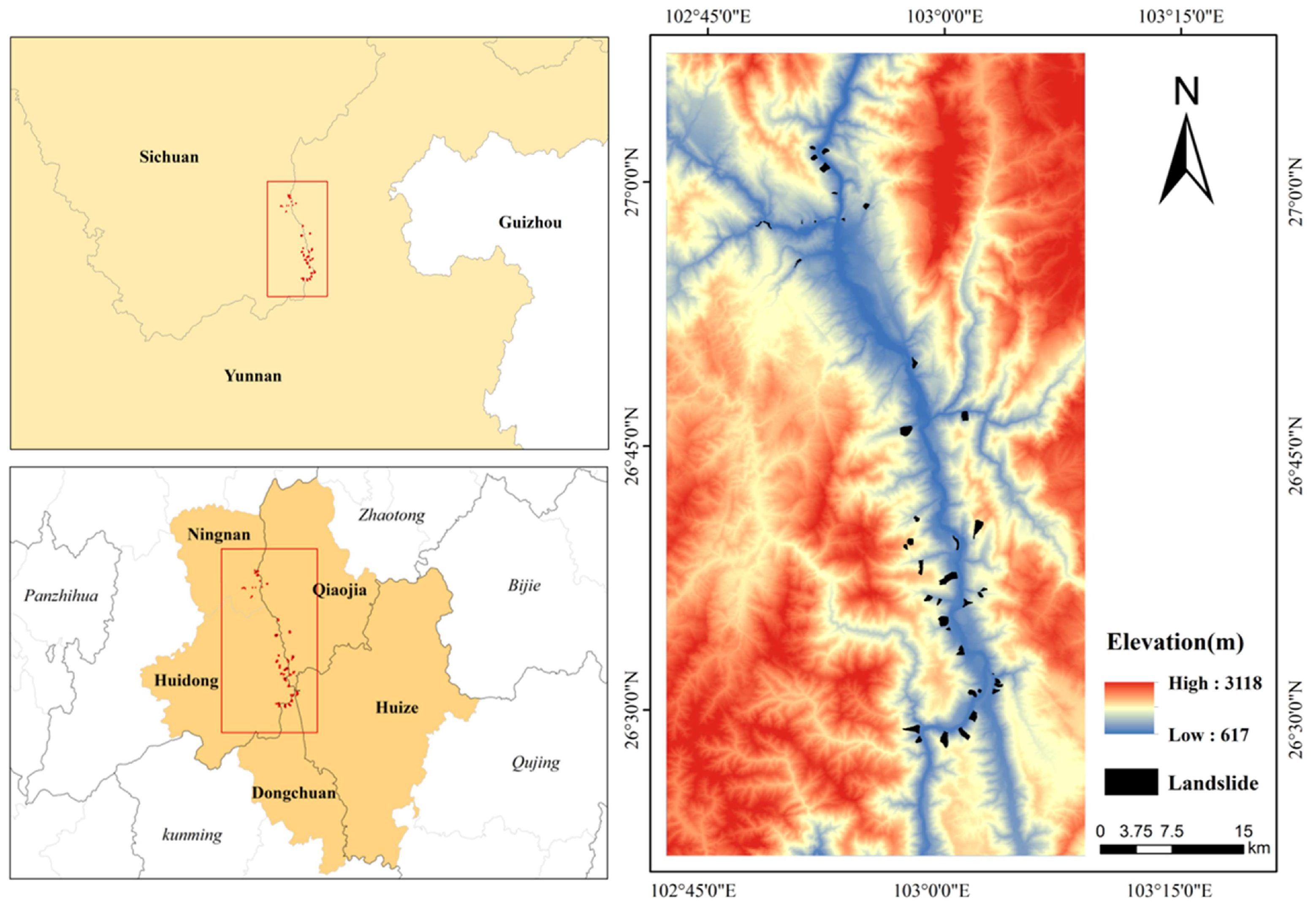
2.1. Study Area

The Baihetan Reservoir Area (BRA) is located in the border area between Sichuan Province and Yunnan Province in China, adjacent to five counties (districts): Huidong County, Ningnan County, Qiaojia County, Huize County, and Dongchuan District (Figure 1). This region lies between the Wumeng Mountains and the Lunan Mountains within the Hengduan Mountains, positioned on the southeastern edge of the Qinghai Tibet Plateau. It falls within the high mountain and plateau geomorphic units of southwestern Sichuan and northeastern Yunnan. The terrain exhibits significant variations, marked by complexity, with most mountain peaks surpassing an elevation of 2000 m. The BRA is situated in the Jinsha River Basin, encompassing a broad distribution of water systems, including tributaries such as Xiaojiang River and Pudu River, along with well-developed gullies. This area experiences a typical subtropical humid and alpine climate due to its undulating terrain, high mountains, deep valleys, and abundant precipitation. The combination of these factors makes it susceptible to elevated river water levels, impacting steep terrain and unstable slope. The dynamic geological environment and intricate water system contribute to the BRA being a high-risk area for landslide disasters [31]. Consequently, effective identification and analysis of landslides in this area are paramount for proactive prevention and response measures.

2.2. Data and Preprocessing

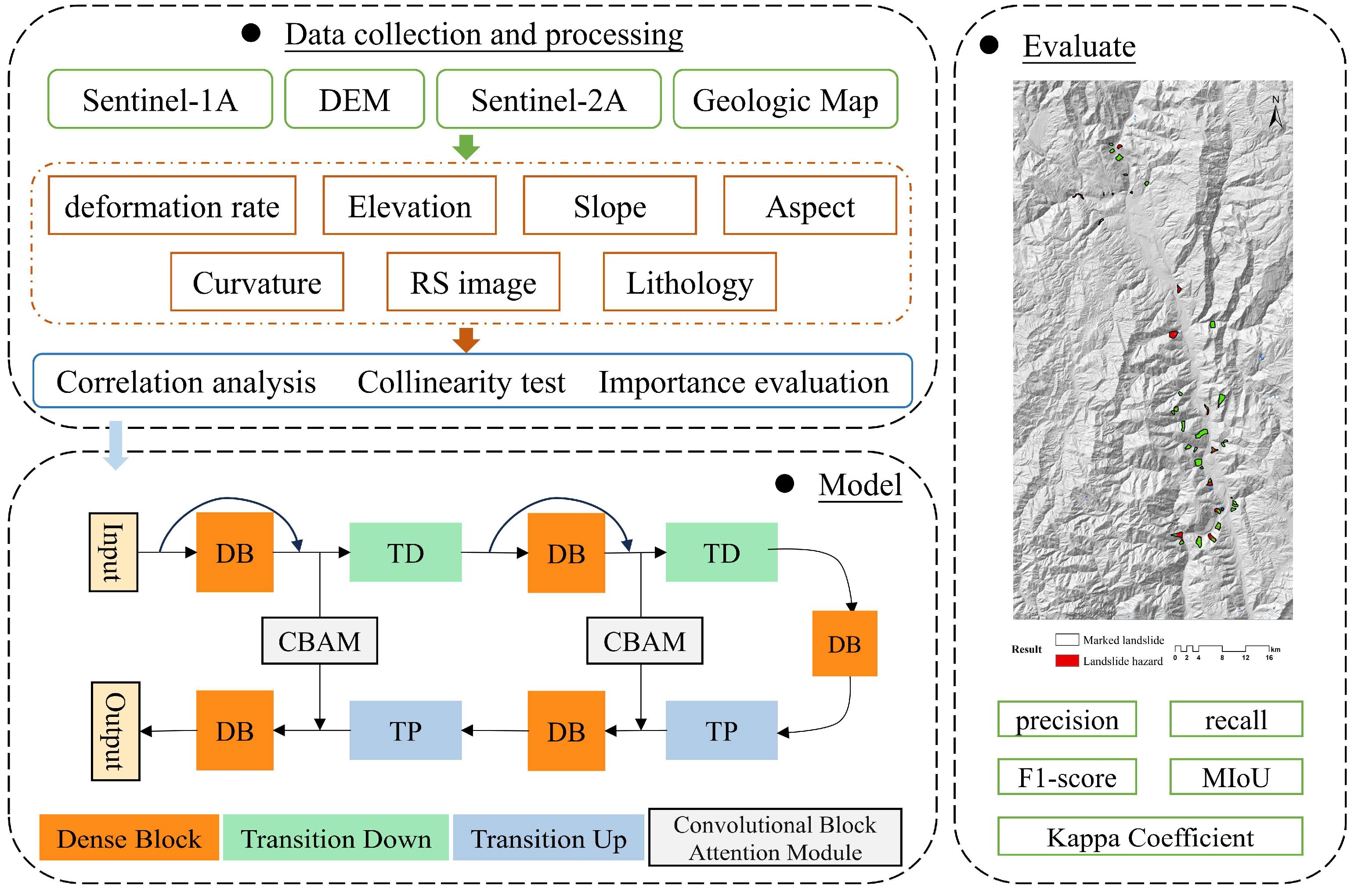
In order to detect landslides in the BRA, this study mainly collected Sentinel-1 images to offer surface deformation information, Sentinel-2 images to provide surface feature details. Digital elevation model (DEM) and regional geological maps, as well as derived factors were incorporated to furnish geological structure information.

Table 1. Data information.

Data	Information	Number/Cloud Coverage	Resolution	Data Source
Sentinel-1	9 January 2021–29 May 2023	103 scenes	5 m × 20 m	European Space Agency
Sentinel-2	20230529T034541_T48RTR	0.7637%	10 m
	20230529T034541_T48RUR	1.2485%
	20230521T033539_T48RTQ	0.0565%
	20230521T033539_T48RUQ	0.4099%
DEM	/		12.5 m	Alaska Satellite Facility
Lithology	/		/	Geologic Map

outlines the main data sources and information utilized in this study.

The deformation data in this study are derived from Sentinel-1 image provided by the European Space Agency. Sentinel-1A possesses all-weather observation capabilities, making it widely used in surface monitoring [32]. SBAS-InSAR, employed in this study, is an InSAR time series analysis technique based on multiple main images [33]. Its principle involves calculating the time and spatial baselines of multi-scene SAR images in different time periods within the coverage area. Subsequently, differential interference processing and phase unwrapping are performed on the selected interference pairs. A series of subsets are generated based on the time and spatial baselines, and the least squares method is used to estimate deformation parameters. The final step involves inversion calculation and geocoding to obtain deformation results. To ensure the data source base for SBAS-InSAR technology processing and the accuracy of obtaining surface deformation information in the study area, 103 Sentinel-1A images from 9 January 2021 to 29 May 2023, were selected. The imaging mode was interferometric wideband imaging (IW) with a resolution of 5 m × 20 m, a central incidence angle of 39.17° and VV single polarization mode. In the SBAS-InSAR method, the threshold for time baseline and spatial baseline is 60 days and 0–2%, respectively. With these limitations, a total of 310 interferograms are generated from the data, revealing a deformation rate in the study area ranging from −136.52 to 44.14 mm/year, as shown in Figure 2a. Based on the surface deformation results obtained from the above process, we selected the areas with obvious deformation and combined optical and Google Earth images for verification, and delineated landslide samples.

The formation of landslides is a complex outcome involving the interaction of multiple factors. Exploring the relationship between internal and external factors and the occurrence of landslides enhances the accuracy of LR [34]. Therefore, optical images and geological factors were also chosen as landslide causative factors (LCFs), conducting LR together with deformation rate.

Sentinel-2 images are also sourced from the European Space Agency, encompassing a total of 4 scenes across the entire study area, with imaging dates of 21 May 2023 and 29 May 2023. Following preprocessing steps such as radiometric calibration and atmospheric correction, bands 2, 3, 4, and 8 with a resolution of 10 m were selected for band fusion, cropping, and embedding to enhance interpretability. Additionally, the DEM used in this study was obtained from the Alaska Satellite Facility, featuring a spatial resolution of 12.5 m. Given the close relationship between the occurrence of landslide geological disasters and LCFs, this study selected DEM-derived factors such as slope, aspect, curvature, and geological lithology maps as LCFs for LR. All LCFs were underwent processing based on ENVI5.3, SARscape platform and ArcGIS10.7, and the results were visualized using ArcGIS10.7 (Figure 2).

To ensure pixel position matching, the spatial resolution of all factors was resampled to 12.5 m. To standardize the data distribution across different dimensions and expedite the convergence speed of the model, the Z-score method was used to normalize each channel of input data [35]. Given the relatively small proportion of landslide samples, a data augmentation strategy was adopted to generate more training samples. This experiment utilized a sliding window size of 128 × 128 to scan and generate non-overlapping sample blocks. Divide landslide and non-landslide samples at a ratio of 7:3, and then combine 70% of the selected samples into the training dataset to learn landslide characteristics.

3. Method

This study is organized into three main components: data collection and processing, model training, predictive evaluation (Figure 3). The first part is data collection and processing, mainly including radar satellite data collection and processing in the research area, image and deformation data acquisition, sample annotation, and geological factor extraction. The second part is the model construction, a new FCADenseNet model is established based on semantic segmentation, incorporating attention modules. Additionally, three commonly used semantic segmentation networks are selected for comparison. The third part involves predictive evaluation, wherein the trained model is employed to predict the entire research area. Five evaluation metrics (EMs) for assessment of the performance of the LR models, and the LR map are generated based on the predictions.

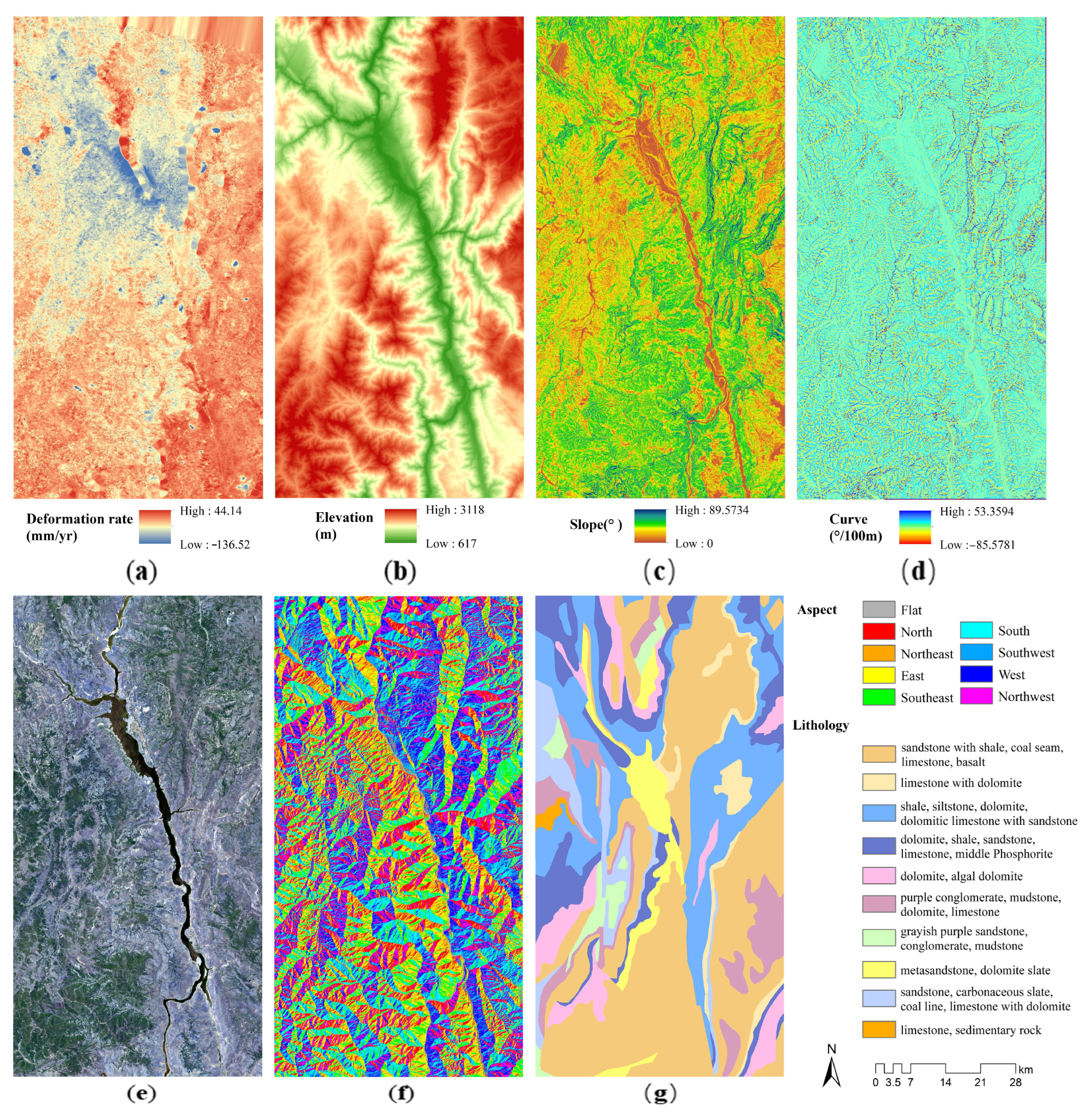
3.1. Selection of LCFs

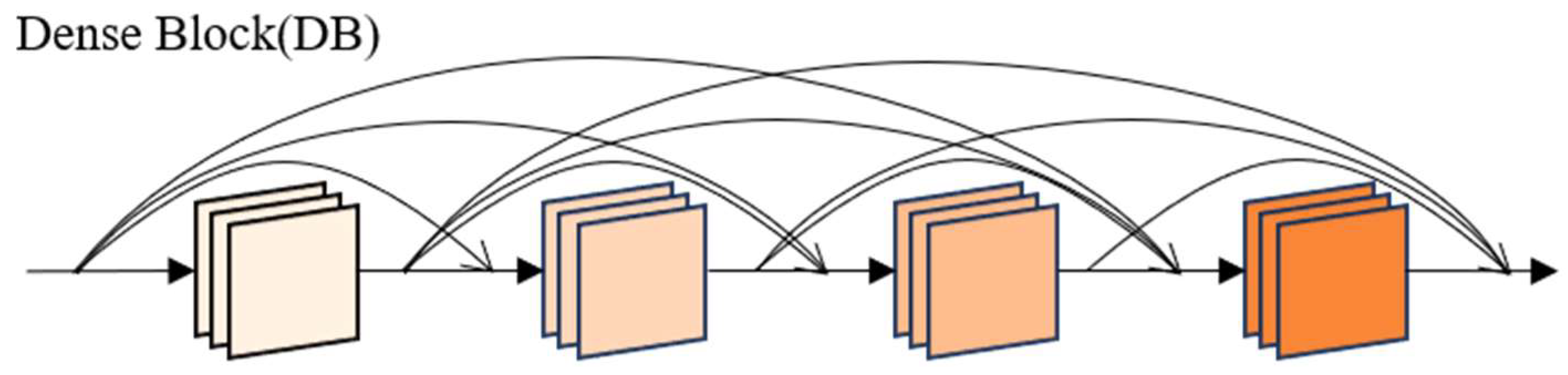
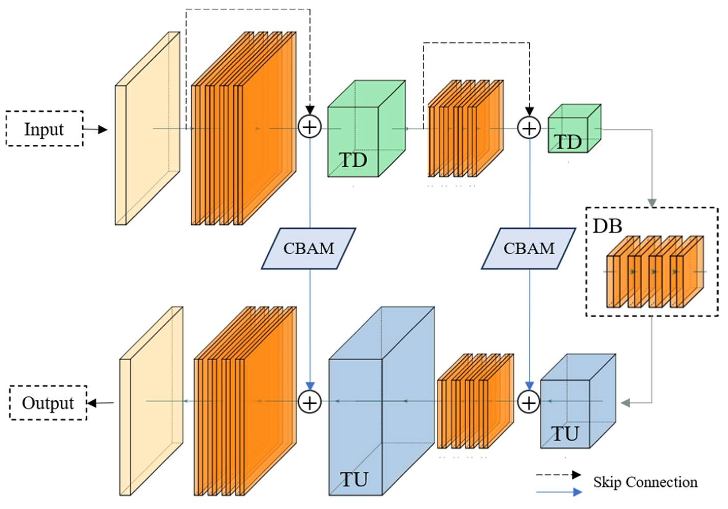
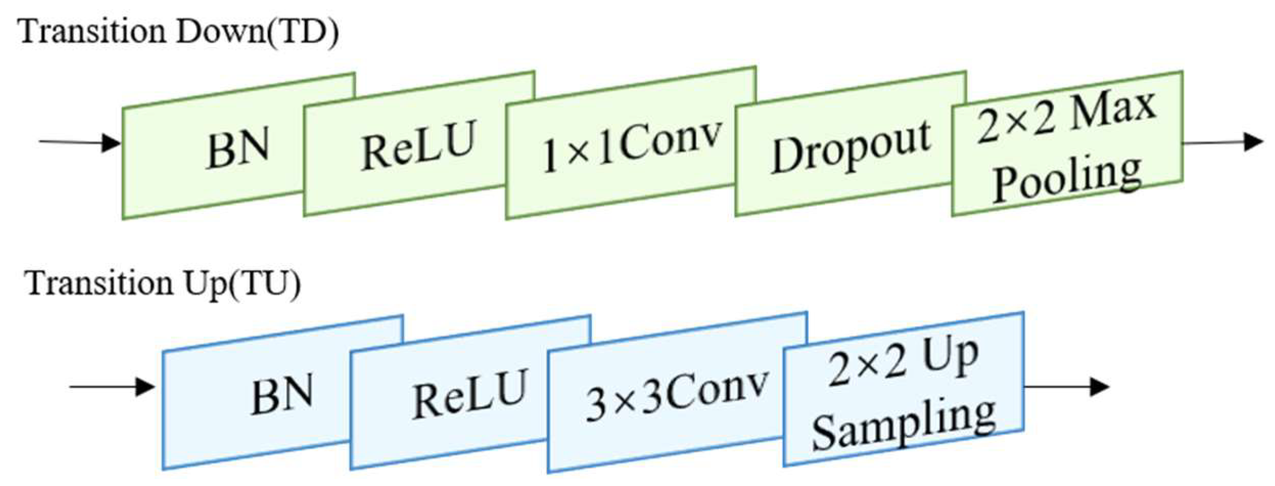
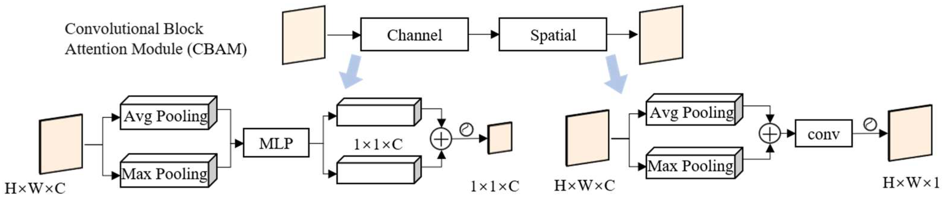
The selection of LCFs has an important impact on the overall performance of the model. When factors exhibit high correlation, indicating a strong linear or non-linear relationship between them, it not only burdens the model with excessive data but also interferes with the weight allocation of different features during the feature learning process [36]. Consequently, this study conducted correlation analysis, collinearity test, and importance evaluation on the LCFs.

(1) Correlation analysis: Pearson correlation coefficient, also known as Pearson product moment correlation coefficient (PPMCC), serves as a metric for quantifying the linear correlation between two variables, denoted as X and Y. The correlation values range from −1 and 1, indicating the strength and direction of the relationship between the variables [37]. This coefficient is determined by evaluating the covariance and standard deviation of the two sets of data, as illustrated in Formula (1):

$$PPMCC=\frac{cov\left(X,Y\right)}{{\sigma }_X{\sigma }_Y}=\frac{{\sum }_{i=1}^n\left(X_i-\overline{X}\right)\left(Y_i-\overline{Y}\right)}{\sqrt{{\sum }_{i=1}^n{\left(X_i-\overline{X}\right)}^2}\sqrt{{\sum }_{i=1}^n{\left(Y_i-\overline{Y}\right)}^2}}$$

(1)

where n is the total number of samples, and $cov\left(X,Y\right)$ represents the covariance between variables X and Y. Additionally, ${\sigma }_X$, ${\sigma }_Y$ signify the standard deviation of all samples. $\overline{X}$ and $\overline{Y}$ denote the average values of all samples.

(2) Collinearity test: Multicollinearity refers to the linear correlation among independent variables [38]. It involves examining tolerance (TOL) and variance inflation factor (VIT) between selected factors, which exhibit a reciprocal relationship. The calculation method of VIF is shown in Formula (2). The closer the VIF value is to 1, the weaker the correlation among the data, while a higher value indicates a more pronounced correlation.

$$VIF=\frac{1}{1-R_i^2}$$

(2)

where $R_i^2$ represents the $i$-th variable and obtains the corresponding decision coefficient in the linear regression model.

(3) Importance evaluation: Factors have different contributions to the performance of the model, and the importance of LCFs is ranked using the Gini index in the random forest model [39]. If a feature is frequently selected for node partitioning in the construction of random forests and can improve model performance after partitioning, then this feature is likely to be an important feature. Conversely, if a feature is rarely selected in the construction of a random forest or has little impact on model performance after partitioning, then this feature is likely to be an unimportant feature. By employing this approach, we can rank the importance of features.

3.2. FCADenseNet

The model initially incorporates fundamental concepts from DenseNet and ResNet, establishing connections between feature maps (FMs) at different levels through dense connections. This design enables each layer to directly access information from all previous layers. Simultaneously, the incorporation of residual connections aims to address the gradient dispersion problem that may arise with deepening the network. The architecture of the FCN encoder–decoder is subsequently retained, transforming the conventional DenseNet into a model well suited for image segmentation tasks. This adaptation allows for the generation of pixel-level segmentation predictions, effectively fusing spatial characteristics [40].

However, the dense feature reuse and connections may result in the loss of original information. Moreover, the smoothing and interpolation operations during the up-sampling process can cause the blurring of edge information. Although the model’s emphasis on learning deep semantic information, it is crucial to preserve detailed information. Consequently, an attention module is introduced to both the decoding and encoder skip connection sections, with the weight adjusted to learn without unduly increasing the model’s complexity. This strategic enhancement aims to better leverage low-level fine information and high-level semantic features. Figure 4 shows the overall model structure.

The FCADenseNet model mainly consists of four modules: Dense Block (DB), Transition Down (TD), Transition Up (TU), and attention mechanism. In the DB, the FMs of each layer are densely connected to the FMs of all previous layers, to facilitating optimal information transmission (Figure 5). This dense connection method significantly augments the number of connections in the network, allowing each layer to directly access information from all previous layers. Leveraging features from previous layers enhances the expression ability of each layer, resulting in the extraction of richer semantic information. The formula governing this process is as follows:

$$X_L=F_l\left(\left[X_0,X_1,\dots ,X_{L-1}\right]\right)$$

(3)

where $\left[X_0,X_1,\cdots ,X_{L-1}\right]$ refers to the dense connections of the FMs of layers 0,…, L − 1. $F_l$ represents a combination of non-linear transformation functions: three operations are batch normalization (BN), ReLU activation function, and 3 × 3 Convolution convolutions [41,42].

Following the dense connections, each layer $F_l$ produces k FMs, referred to as growth rates, which are hyperparameters. Generally, opting for a smaller k tends to yield superior performance. To mitigate an upsurge in feature computation due to redundant learning, an internal 1 × 1 convolutional bottleneck layer is incorporated for feature compression.

The TD module employs a convolution operation akin to the DB module. It is distinguished by reducing the number of channels in the FM through a 1 × 1 convolution layer and a max-pooling operation, effectively diminishing reducing network parameters. In the decoder, TD and DB modules are arranged alternately, facilitating the extraction of global information from the input data. The decoder part is a combination of TU and DB modules. The TU module uses 3 × 3 convolutional layers and 2 × 2 up-samplingup-sampling layers to systematically restore low resolution FMs to their original resolution. The overall structure is shown in Figure 6.

Spectral and spatial features contained in different terrain characteristics in RS data are represented differently in FMs. The recognition ability will be greatly improved by pinpointing significant features of landslide objects in specific bands and spatial dimensions. To optimize the utilization of both low-level fine information and high-level semantic features, the Convolutional Block Attention Module (CBAM) [43] has been introduced to the shallow FMs in the skip connection section after the TU module. It is an efficient module suitable for feedforward neural networks, where the given feature map infers the attention map along two independent dimensions, and then multiplies the attention map with the input feature map for adaptive feature optimization. This is achieved through the learning of weights or attention distribution, facilitating the extraction and accentuation of key landmark features [44]. The structure of this attention module is shown in Figure 7. The channel attention component dynamically adjusts the importance level of channels in the FMs, while the spatial attention part underscores the significance of spatial positions in the FMs, and the pooling operation can generate information feedback for each pixel. By focusing on these key features, the information contained in the shallow FMs is emphasized, effectively mitigating information loss caused by the up-sampling process in the FM and improving overall model performance. Ultimately, the class distribution of each pixel is derived through sigmoid non-linear mapping.

3.3. Evaluation Metrics

Five commonly used evaluation metrics (EMs) were chosen to quantitatively evaluate the performance of the proposed LR method. These metrics include the precision (Pre), recall (Rec), F1-score (F1), Kappa coefficient (Kappa), and mean intersection over union (MIoU). These five EMs are defined as follows.

Pre refers to the proportion of correctly predicted positive samples to the total number of predicted positive samples. Rec refers to the proportion of correctly predicted positive samples to all positive samples. Usually, in order to comprehensively evaluate the performance of classification models, F1 is used to evaluate the model. When F1 is high, the model performs well [45]. The calculation formulas of these three EMs are as follows:

$$Pre=\frac{TP}{TP+FP}$$

(4)

$$Rec=\frac{TP}{TP+FN}$$

(5)

$$F1=2\times \frac{Pre\times Rec}{Pre+Rec}$$

(6)

where TP is the number of correctly predicted positive samples, TN is the number of correctly predicted negative samples, FN is the number of predicted negative samples, and FP is the number of predicted positive negative samples.

Kappa coefficient is a method of evaluating consistency, ranging from [–1, 1]. The higher the value of the coefficient, the higher the classification accuracy achieved by the model [46]. Kappa coefficient and overall accuracy are mutually verified, and the results are objectively evaluated. The formula is as follows:

$$kappa=\frac{p_o-p_e}{1-p_e}$$

(7)

$$p_o=\frac{TP+TN}{TP+TN+FP+FN}$$

(8)

$$p_e=\frac{\left(TP+FN\right)\left(TP+FP\right)+\left(FP+TN\right)\left(FN+TN\right)}{n^2}$$

(9)

MIoU calculates the ratio of the intersection and union of pixels in each category, and averages the results of all categories to obtain the final MIoU value [47]. When the true and predicted values are the same, the MIoU value is 1, indicating a perfect match in an ideal situation. The formula is as follows:

$$MIoU=\frac{1}{2}\times \left(\frac{TP}{TP+FN+FP}+\frac{TN}{TN+FN+FP}\right)$$

(10)

3.4. Experiment Setting

The construction of the experimental platform mainly includes three key aspects: hardware configuration, running environment setup, and parameter settings. The experimental code was written using the Python programming language, executed on the Pycharm2021 software, and built upon the Keras framework within TensorFlow. Firstly, the network weights are randomly initialized. The classifier of the network uses the sigmoid function, which is suitable for binary classification problems. The binary cross-entropy function is chosen as the loss function for LR. Using Adam algorithm as the optimization algorithm, the learning rate is 0.0001, the batch size is 8, and the network weights are fine tuned. Additionally, a Dropout layer with a value of 0.2 is incorporated during training to streamline the model and mitigate gradient disappearance. Finally, the ModelCheckpoint function is selected to monitor changes in the loss function and automatically save the model.

4. Results and Analysis

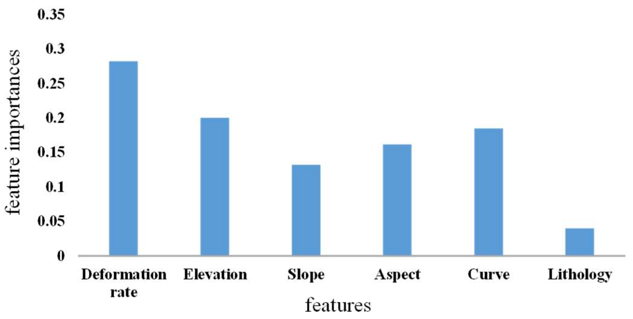
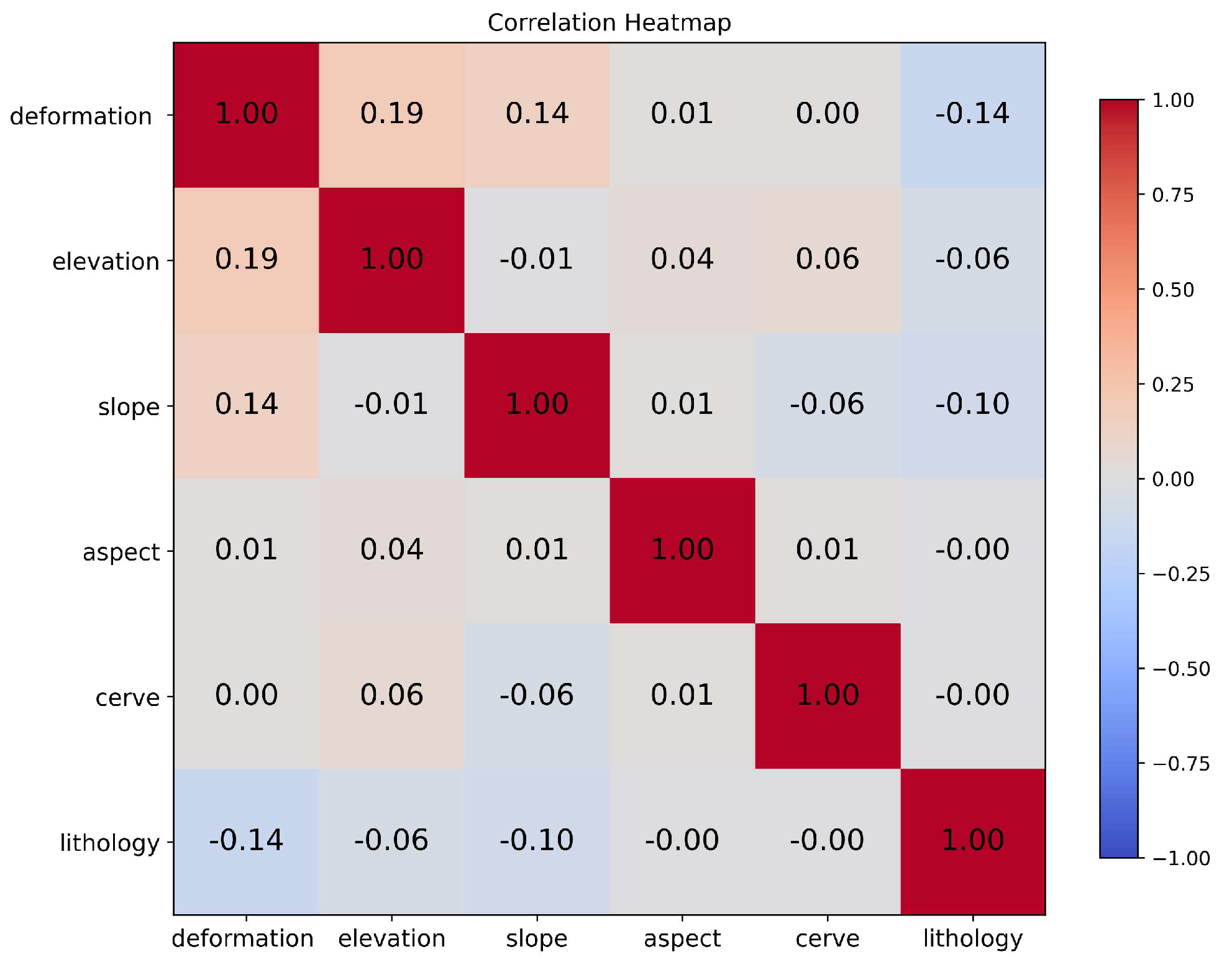
4.1. Analysis of LCFs

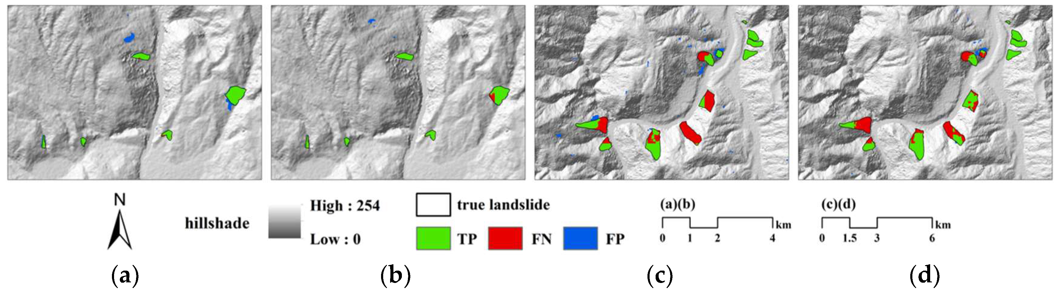
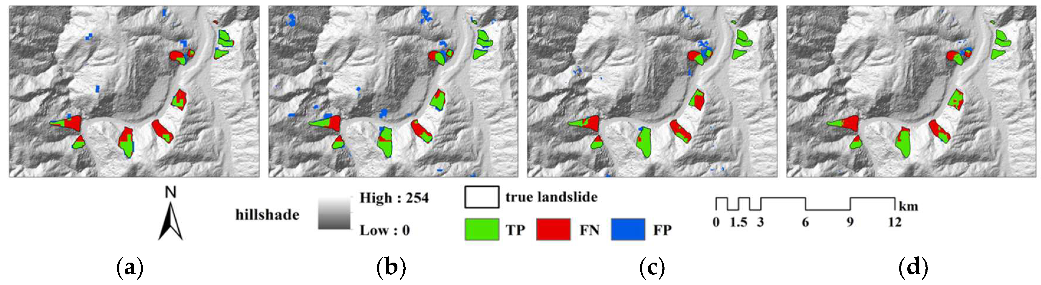
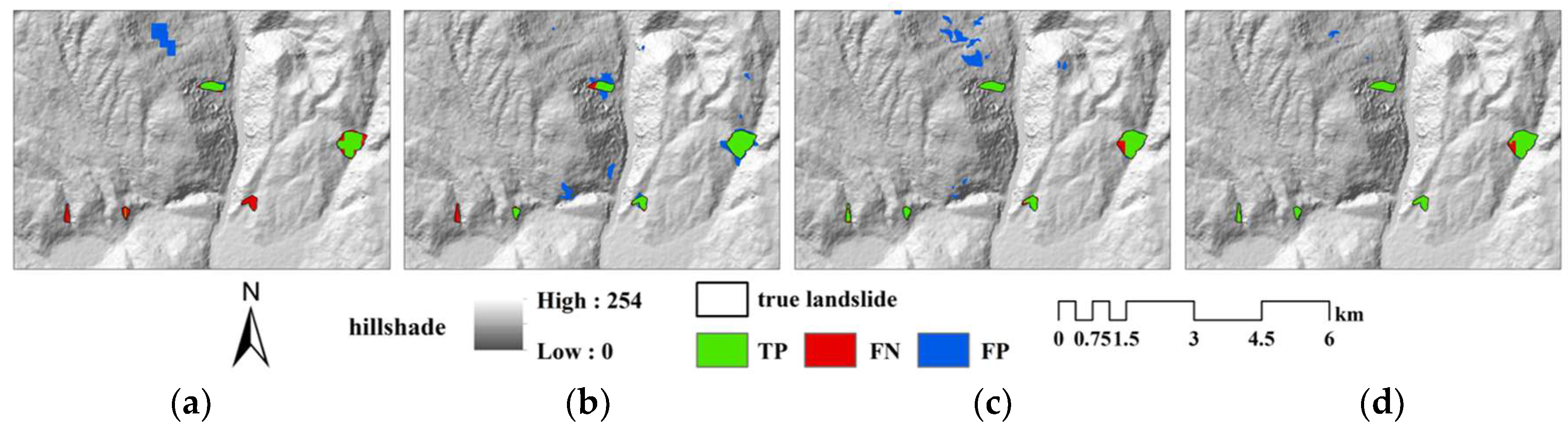
In this study, PyCharm 2020 was employed to calculate correlations, VIF, and TOL among the selected factors. Figure 8 shows the PPMCC visualization thermal map of six LCFs in the study area, including deformation rate. Positive and negative values represent the positive and negative correlation between the data, while the depth of the color indicates the strength of these correlations. Specifically, the deformation rate is positively correlated with elevation and slope features, with correlation coefficients of 0.19 and 0.14, respectively. It indicates that with the increase in height and slope in the region, the rate of surface deformation also rises. Relatively high elevations and steep slopes have a certain correlation with the occurrence of landslide events, which is reflected in surface deformation. Consequently, selecting elevation and slope features as discriminant factors proves beneficial for LR.

Table 2. Multicollinearity test results of factors.

	Deformation Rate	Elevation	Slope	Aspect	Curve	Lithology
VIF	1.074	1.044	1.031	1.002	1.007	1.028
TOL	0.931	0.957	0.970	0.998	0.993	0.973

shows the VIF and TOL values for the six LCFs. The results indicate a weak positive correlation among the selected LCFs. The VIF and TOL values for each LCF approach 1, indicating that the correlation among the selected LCFs in this study is not strong. There is no need for removal through multicollinearity testing, affirming the robustness of the chosen factors in the analysis.

The importance ranking distribution of each LCFs in the study area is shown in Figure 9, with the highest importance value for surface deformation rate, followed by elevation and curvature. A high deformation rate indicates the acceleration or rapid subsidence of geological bodies, and a high probability indicates the occurrence of landslides; Elevation and curvature are also important factors in the occurrence of landslides. Stress concentration at high curvature and steep slopes at high altitudes are more prone to landslides, so their importance is also high. The importance of lithology is the lowest, as there are many kinds of lithology and complex distribution in the region.

4.2. LR Results

In this section, the performance of LR result of the proposed FCADenseNet model are compared with three LR model, which are FCN, U-Net [48], and FC_DenseNet [40] network.

Since the landslide area in the study area occupies a small area, we chose to zoom in on the local area to view the model identification results. As shown in Figure 10 and Figure 11, they belong to two representative areas of medium landslide (most landslides) and small landslide development in the region, respectively. According to the results, for medium landslide, Figure 10a,b, respectively, show the results of the FCN and U-Net models respectively. The FCN model seems to be overly regularized in identifying landslide boundaries, resulting in a noticeable rectangular shape. The U-Net model demonstrates stronger land-slide localization capabilities. But there are some difficulties in distinguishing similar backgrounds around landslides, resulting in incorrect predictions. Figure 10c,d, respectively, show the results of the FC_DenseNet and FCADenseNet models respectively. Considering the localization of landslides and the recovery of boundary features, the results are more accurate compared to the first two models, but there is still some noise in the results of the FC_DenseNet model. The landslide range identified by FCADenseNet in the four model results is more complete, and due to the introduction of attention, it effectively recovers the loss of edge information during the up-sampling process. It is worth noting that for the recognition results of small landslides, the range of landslides annotated based on prior knowledge is very small, and there are obvious differences between the results of models. Figure 11a,b show the identification results of FCN and U-Net models, respectively. FCN and U-Net models are difficult to identify such small landslides. Figure 11c,d show the results of the FC_DenseNet and FCADenseNet models, both of which accurately identify the range of small landslides. In comparison, FCADenseNet has fewer errors in identifying the surrounding areas.

Furthermore, based on the visual results, we quantitatively analyzed the performance of the model using the five EMs. In the experiment, we opted not to use Overall Accuracy (OA) as one EM because the substantial imbalance between non-landslide and landslide pixels in the study area, with a ratio of 224:1. The proportion of non-landslide pixels is very high, which leads to a small change between the OA values of the model. From

Table 3. The EMs of different models (the bold and underlined value means the highest EMs of the col).

	Pre	Rec	F1	Kappa	MIoU
FCN	0.6870	0.5354	0.6018	0.6002	0.7136
U-Net	0.4653	0.6908	0.5561	0.5543	0.6901
FC_DenseNet	0.6312	0.7043	0.6658	0.6599	0.7479
FCADenseNet	0.8381	0.6972	0.7611	0.7602	0.8062

, the five EMs of FCADenseNet are superior to the other three models, achieving commendable LR results. The FCADenseNet model, augmented with an attention module, achieves the Pre of 0.8381, the Rec of 0 6972, the F1 of 0.7611, the kappa of 0.7602, and the MIoU of 0.8062. It is noteworthy that the results of the proposed FCADenseNet obtained the highest values of the five EMs, except for Rec. Compared to the FC_DenseNet model, the F1, Kappa, and MIoU demonstrate improvements of 14.3%, 15.1%, and 7.8%, respectively. This enhancement stems from our introduced method, adjusting the attention weight of the model to preserve shallow information on landslide boundary features, effectively recovering the loss of edge information during the up-sampling process. This adjustment is the main reason for improving model accuracy.

4.3. Improvement of FCADenseNet Performance by Deformation Rate

To verify the impact of deformation rate on the performance of the model, we compared the LR results using the FCADenseNet model with or without deformation rate. Two sets of training datasets were created: RS (devoid of deformation rate) and RS-DR (incorporating deformation rate). The proposed FCADenseNet model was used to evaluate both datasets.

Similarly, we focused on a local area for a closer examination of the model’s LR results. As shown in Figure 12a,b, they represent the LR outcomes of small landslide areas using RS and RS-DR training data, respectively. With sufficient learning from the FCADenseNet model, the recognition of small landslides is relatively accurate, but there is no pronounced increase in error recognition for non-landslide areas. Figure 12c,d represent the recognition results of the local landslide area using RS and RS-DR training data, respectively. The results of this area indicate that the model has some difficulties in identifying the overall range of landslides in this area, but with the addition of deformation rate features, partial positioning can be carried out within the landslide area, and the recognition results have been improved.

Table 4. The EMs of FCADenseNet for two training data (the bold and underlined value means the highest EMs of the col).

	Pre	Rec	F1	Kappa	MIoU
RS	0.6614	0.6878	0.6743	0.6729	0.7529
RS-DR	0.8381	0.6972	0.7611	0.7602	0.8062

presents the quantitative analysis results for the two datasets. When using the RS-DR dataset, the model achieved an F1, a kappa, and a MIoU of 0.7611, 0.7602, and 0.8062, respectively. Compared with the RS dataset, the model exhibited increases in 12.9%, 12.9%, and 7.1% in F1, kappa, and MIoU, respectively, highlighting the practicality of deformation rate in effectively distinguishing landslides. Notably, in the results from both datasets, the Rec value did not exhibit significant changes, while the Pre value demonstrated a notable improvement. Combining the results of Figure 12, it becomes evident that the RS-DR dataset provides a more detailed depiction of the morphology of localized landslide, resulting in clearer LR results. This indicates that adding deformation rate as a landslide feature has a positive effect on LR.

5. Discussion

5.1. Comparisions of the Model’s Effect

Currently, LR methods based on semantic segmentation usually adopt an encoding–decoding structure. In this structure, the stacking of convolutional layers can extract landslide-related information well. However, during the up-sampling process, the gradual recovery of feature maps may lead to the loss of information. To solve this problem, the FCADenseNet proposed in this article adds an attention mechanism module based on the original model and applies it to skip connections. This attention mechanism module focuses on the information contained in the shallow feature map, effectively reducing the information loss that may occur during the sampling process on the feature map. According to comparative experiments with the original FC_DenseNet, U-Net, and FCN networks, the FCADenseNet model has a more complete landslide boundary in terms of landslide recognition effect, and has stronger recognition capabilities for some small landslides. This adjustment effectively maintains the integrity of the original features during the information recovery process and is the main factor in improving model accuracy.

5.2. Influence of Deformation Rate on LR

In the BRA, the water level of the river undergoes constant changes due to factors such as rainfall and reservoir water storage. Additionally, the slope of the reservoir area experiences continuous fluctuations. To account for these variations, we incorporate a time series deformation change value, integrating it into LCFs to train the model for LR. Given that the FCADenseNet model has already demonstrated excellent LR results, we conducted a comparative analysis to assess the impact of including deformation rate features. The results indicate that, when deformation rate is combined, the model can more accurately identify landslide. However, some challenges remain, particularly in achieving precise landslide positioning. There are regional landslides in the results that have not been recognized by all models in this study, but there are in the sample library, which may be due to incorrect labeling of samples based on deformation results and images; and the “false detection” areas in the identification results may have some impact on the quantitative evaluation results because these areas have characteristics of landslide hazards but are not in our original sample library. Addressing this issue requires ongoing attention to surface deformation conditions, with on-site verification being crucial for subsequent research endeavors. In addition, it is difficult to accurately analyze the motion characteristics of some deep landslides solely through InSAR methods. The surface deformation rate characteristics have a certain improvement effect on the recognition of these shallow landslides, but the impact on deep landslides still needs to be explored.

5.3. Limitations and Future Work

This study attempts to combine landslide surface deformation with DLAs for landslide disaster recognition However, practical applications still face challenges in timely LR. Firstly, the orbital data of the Sentinel-1A satellite can be used to provide surface deformation data for LR. However, effectively analyzing orbit and descent data, leveraging richer SAR data resources such as interferograms, and fusing InSAR data into factor data in a more appropriate manner is still an unresolved issue. This is crucial for monitoring surface deformation with higher accuracy and obtaining more precise landslide cataloging data. Secondly, the utilization of DLAs requires a substantial amount of sample data to ensure accuracy, rendering it more suitable for ongoing landslides that require long-term monitoring. Research efforts should focus on establishing dynamic databases that can be updated in real time, thereby enhancing the generalization ability of existing models.

6. Conclusions

In this study, we aimed to validate the feasibility of combining InSAR technology with deep learning in LR. We obtained the annual deformation rate of the BRA as the main factor using SBAS-InSAR technology. This information, combined with the study area image and geological factors, formed a new dataset for LR. We constructed a newly Dense Connected Fully Convolutional Network model, incorporating an attention mechanism, FCADenseNet, for LR. To assess the performance of the model, comparisons were made with FCN, U-Net, and FC_DenseNet networks. The results demonstrate that the proposed FCADenseNet achieves the F1-score of 0.7611 and the kappa of 0.7602, which is more effective in this study and has certain advantages for small landslides. We also analyzed the impact of surface deformation rate on LR. The results indicate that the increase in surface deformation characteristics has a positive impact on LR. In the future, the integration of InSAR technology with the existing system will provide more timely information for the monitoring and rapid identification of landslide disasters. The establishment of a long-term dynamic database will play a proactive role in regional disaster monitoring and recognition.

References

1. Casagli, N.; Intrieri, E.; Tofani, V.; Gigli, G.; Raspini, F. Landslide Detection, Monitoring and Prediction with Remote-Sensing Techniques. Nat. Rev. Earth Environ. 2023, 4, 51–64. [Google Scholar] [CrossRef]
2. Lissak, C.; Bartsch, A.; De Michele, M.; Gomez, C.; Maquaire, O.; Raucoules, D.; Roulland, T. Remote Sensing for Assessing Landslides and Associated Hazards. Surv. Geophys. 2020, 41, 1391–1435. [Google Scholar] [CrossRef]
3. Gao, J.; Sang, Y. Identification and Estimation of Landslide-Debris Flow Disaster Risk in Primary and Middle School Campuses in a Mountainous Area of Southwest China. Int. J. Disaster Risk Reduct. 2017, 25, 60–71. [Google Scholar] [CrossRef]
4. Catani, F. Landslide detection by deep learning of non-nadiral and crowdsourced optical images. Landslides 2021, 18, 1025–1044. [Google Scholar] [CrossRef]
5. Mohan, A.; Singh, A.K.; Kumar, B.; Dwivedi, R. Review on remote sensing methods for landslide detection using machine and deep learning. Trans. Emerg. Telecommun. Technol. 2021, 32, e3998. [Google Scholar] [CrossRef]
6. Du, B.; Zhang, W. Research on object-oriented high resolution remote sensing image classification technology. West. Resour. 2016, 5, 135–138. [Google Scholar]
7. Long, L.; He, F.; Liu, H. The use of remote sensing satellite using deep learning in emergency monitoring of high-level landslides disaster in Jinsha River. J. Supercomput. 2021, 77, 8728–8744. [Google Scholar] [CrossRef]
8. Das, R.; Wegmann, K.W. Evaluation of Machine Learning-Based Algorithms for Landslide Detection across Satellite Sensors for the 2019 Cyclone Idai Event, Chimanimani District, Zimbabwe. Landslides 2022, 19, 2965–2981. [Google Scholar] [CrossRef]
9. Chen, F.; Yu, B.; Li, B. A Practical Trial of Landslide Detection from Single-Temporal Landsat8 Images Using Contour-Based Proposals and Random Forest: A Case Study of National Nepal. Landslides 2018, 15, 453–464. [Google Scholar] [CrossRef]
10. Krawczyk, B.; Woźniak, M.; Schaefer, G. Cost-Sensitive Decision Tree Ensembles for Effective Imbalanced Classification. Appl. Soft Comput. 2014, 14, 554–562. [Google Scholar] [CrossRef]
11. Ding, A.; Zhang, Q.; Zhou, X.; Dai, B. Automatic recognition of landslide based on CNN and texture change detection. In Proceedings of the 2016 31st Youth Academic Annual Conference of Chinese Association of Automation (YAC), Wuhan, China, 11–13 November 2016; pp. 444–448. [Google Scholar]
12. Simonyan, K.; Zisserman, A. Very Deep Convolutional Networks for Large-Scale Image Recognition. In Proceedings of the 2015 IEEE Conference on Computer Vision and Pattern Recognition (CVPR), Boston, MA, USA, 7–12 June 2015; pp. 509–518. [Google Scholar]
13. He, K.; Zhang, X.; Ren, S.; Sun, J. Deep Residual Learning for Image Recognition. In Proceedings of the 2016 IEEE Conference on Computer Vision and Pattern Recognition (CVPR), Las Vegas, NV, USA, 27–30 June 2016; pp. 770–778. [Google Scholar]
14. Chen, T.; Gao, X.; Liu, G.; Wang, C.; Zhao, Z.; Dou, J.; Niu, R.Q.; Plaza, A. BisDeNet: A New Lightweight Deep Learning-based Framework for Efficient Landslide Detection. IEEE J. Sel. Top. Appl. Earth Obs. Remote Sens. 2024, 17, 3648–3663. [Google Scholar] [CrossRef]
15. Shelhamer, E.; Long, J.; Darrell, T. Fully Convolutional Networks for Semantic Segmentation. IEEE Trans. Pattern Anal. Mach. Intell. 2017, 39, 640–651. [Google Scholar] [CrossRef] [PubMed]
16. Ronneberger, O.; Fischer, P.; Brox, T. U-Net: Convolutional Networks for Biomedical Image Segmentation. In Medical Image Computing and Computer-Assisted Intervention—MICCAI 2015; Navab, N., Hornegger, J., Wells, W.M., Frangi, A.F., Eds.; Lecture Notes in Computer Science; Springer International Publishing: Cham, Switzerland, 2015; Volume 9351, pp. 234–241. [Google Scholar]
17. Lei, T.; Zhang, Y.; Lv, Z.; Li, S.; Liu, S.; Nandi, A.K. Landslide Inventory Mapping from Bitemporal Images Using Deep Convolutional Neural Networks. IEEE Geosci. Remote Sens. Lett. 2019, 16, 982–986. [Google Scholar] [CrossRef]
18. Liu, P.; Wei, Y.; Wang, Q.; Chen, Y.; Xie, J. Research on Post-Earthquake Landslide Extraction Algorithm Based on Improved U-Net Model. Remote Sens. 2020, 12, 894. [Google Scholar] [CrossRef]
19. Soares, L.P.; Dias, H.C.; Grohmann, C.H. Landslide Segmentation with U-Net: Evaluating Different Sampling Methods and Patch Sizes. arXiv 2020, arXiv:2007.06672. [Google Scholar]
20. Qi, W.; Wei, M.; Yang, W.; Xu, C.; Ma, C. Automatic Mapping of Landslides by the ResU-Net. Remote Sens. 2020, 12, 2487. [Google Scholar] [CrossRef]
21. Gorsevski, P.V.; Brown, M.K.; Panter, K.; Onasch, C.M.; Simic, A.; Snyder, J. Landslide Detection and Susceptibility Mapping Using LiDAR and an Artificial Neural Network Approach: A Case Study in the Cuyahoga Valley National Park, Ohio. Landslides 2016, 13, 467–484. [Google Scholar] [CrossRef]
22. Peduto, D.; Santoro, M.; Aceto, L.; Borrelli, L.; Gullà, G. Full Integration of Geomorphological, Geotechnical, A-DInSAR and Damage Data for Detailed Geometric-Kinematic Features of a Slow-Moving Landslide in Urban Area. Landslides 2021, 18, 807–825. [Google Scholar] [CrossRef]
23. Rosi, A.; Tofani, V.; Tanteri, L.; Stefanelli, C.T.; Agostini, A.; Catani, F.; Casagli, N. The new landslide inventory of Tuscany (Italy) updated with PS-InSAR: Geomorphological features and landslide distribution. Landslides 2018, 15, 5–19. [Google Scholar] [CrossRef]
24. Zhao, F.; Meng, X.; Zhang, Y.; Chen, G.; Su, X.; Yue, D. Landslide susceptibility mapping of karakorum highway combined with the application of SBAS-InSAR technology. Sensors 2019, 19, 2685. [Google Scholar] [CrossRef] [PubMed]
25. Liu, X.; Zhao, C.; Zhang, Q.; Lu, Z.; Li, Z. Deformation of the Baige Landslide, Tibet, China, Revealed Through the Integration of Cross-Platform ALOS/PALSAR-1 and ALOS/PALSAR-2 SAR Observations. Geophys. Res. Lett. 2020, 47, e2019GL086142. [Google Scholar] [CrossRef]
26. Dai, C.; Li, W.; Wang, D.; Lu, H.; Xu, Q.; Jian, J. Active Landslide Detection Based on Sentinel-1 Data and InSAR Technology in Zhouqu County, Gansu Province, Northwest China. J. Earth Sci. 2021, 32, 1092–1103. [Google Scholar] [CrossRef]
27. Lattari, F.; Rucci, A.; Matteucci, M. A Deep Learning Approach for Change Points Detection in InSAR Time Series. IEEE Trans. Geosci. Remote Sens. 2022, 60, 1–16. [Google Scholar] [CrossRef]
28. Cai, J.; Liu, G.; Jia, H.; Zhang, B.; Wu, R.; Fu, Y.; Xiang, W.; Mao, W.; Wang, X.; Zhang, R. A New Algorithm for Landslide Dynamic Monitoring with High Temporal Resolution by Kalman Filter Integration of Multiplatform Time-Series InSAR Processing. Int. J. Appl. Earth Obs. Geoinf. 2022, 110, 102812. [Google Scholar] [CrossRef]
29. Liu, Y.; Yang, H.; Wang, S.; Xu, L.; Peng, J. Monitoring and Stability Analysis of the Deformation in the Woda Landslide Area in Tibet, China by the DS-InSAR Method. Remote Sens. 2022, 14, 532. [Google Scholar] [CrossRef]
30. Zheng, X.; He, G.; Wang, S.; Wang, Y.; Wang, G.; Yang, Z.; Yu, J.; Wang, N. Comparison of Machine Learning Methods for Potential Active Landslide Hazards Identification with Multi-Source Data. ISPRS Int. J. Geo-Inf. 2021, 10, 253. [Google Scholar] [CrossRef]
31. Liu, M.; Yang, Z.; Xi, W.; Guo, J.; Yang, H. InSAR-Based Method for Deformation Monitoring of Landslide Source Area in Baihetan Reservoir, China. Front. Earth Sci. 2023, 11, 1253272. [Google Scholar] [CrossRef]
32. Oludare, O.; Kazeem, R.; Adebayo, A.; Awonusi, A.; Dare, A.; Ikumapayi, O.; Adaramola, B. An Assessment of Earthquake-Induced Landslides Distribution in Nepal Using Open-Source Applications on Sentinel-1 Tops SAR Imagery. Int. J. Des. Nat. Ecodyn. 2023, 18, 237–249. [Google Scholar] [CrossRef]
33. Berardino, P.; Fornaro, G.; Lanari, R.; Sansosti, E. A new algorithm for surface deformation monitoring based on small baseline differential SAR interferograms. IEEE Trans. Geosci. Remote Sens. 2002, 40, 2375–2383. [Google Scholar] [CrossRef]
34. Liu, T.; Chen, T.; Niu, R.; Plaza, A. Landslide Detection Mapping Employing CNN, ResNet, and DenseNet in the Three Gorges Reservoir, China. IEEE J. Sel. Top. Appl. Earth Obs. Remote Sens. 2021, 14, 11417–11428. [Google Scholar] [CrossRef]
35. Lv, Z.; Liu, T.; Shi, C.; Benediktsson, J.A. Local Histogram-Based Analysis for Detecting Land Cover Change Using VHR Remote Sensing Images. IEEE Geosci. Remote Sens. Lett. 2021, 18, 1284–1287. [Google Scholar] [CrossRef]
36. Varmuza, K.; Filzmoser, P. Introduction to Multivariate Statistical Analysis in Chemometrics; CRC Press: Boca Raton, FL, USA, 2016. [Google Scholar]
37. Gulick, S.P.S.; Barton, P.J.; Christeson, G.L.; Morgan, J.V.; McDonald, M.; Mendoza-Cervantes, K.; Pearson, Z.F.; Surendra, A.; Urrutia-Fucugauchi, J.; Vermeesch, P.M.; et al. Importance of Pre-Impact Crustal Structure for the Asymmetry of the Chicxulub Impact Crater. Nat. Geosci. 2008, 1, 131–135. [Google Scholar] [CrossRef]
38. Berk, K.N. Tolerance and Condition in Regression Computations. J. Am. Stat. Assoc. 1977, 72, 863–866. [Google Scholar]
39. Boulesteix, A.-L.; Bender, A.; Lorenzo Bermejo, J.; Strobl, C. Random Forest Gini Importance Favours SNPs with Large Minor Allele Frequency: Impact, Sources and Recommendations. Brief. Bioinform. 2012, 13, 292–304. [Google Scholar] [CrossRef] [PubMed]
40. Gao, X.; Chen, T.; Niu, R.; Plaza, A. Recognition and Mapping of Landslide Using a Fully Convolutional DenseNet and Influencing Factors. IEEE J. Sel. Top. Appl. Earth Obs. Remote Sens. 2021, 14, 7881–7894. [Google Scholar] [CrossRef]
41. Ghorbanzadeh, O.; Blaschke, T.; Gholamnia, K.; Meena, S.; Tiede, D.; Aryal, J. Evaluation of Different Machine Learning Methods and Deep-Learning Convolutional Neural Networks for Landslide Detection. Remote Sens. 2019, 11, 196. [Google Scholar] [CrossRef]
42. Xiao, X.; Lian, S.; Luo, Z.; Li, S. Weighted Res-UNet for High-Quality Retina Vessel Segmentation. In Proceedings of the 2018 9th International Conference on Information Technology in Medicine and Education (ITME), Hangzhou, China, 19–21 October 2018; pp. 327–331. [Google Scholar]
43. Woo, S.; Park, J.; Lee, J.-Y.; Kweon, I.S. CBAM: Convolutional Block Attention Module. Eur. Conf. Comput. Vis. 2018, 11211, 3–19. [Google Scholar]
44. Babak, M.; Dominik, S.; Andreas, U. PRNU-Based Finger Vein Sensor Identification in the Presence of Presentation Attack Data; Verlag der Technischen Universität Graz: Graz, Austria, 2019. [Google Scholar]
45. Ghorbanzadeh, O.; Crivellari, A.; Ghamisi, P.; Shahabi, H.; Blaschke, T. A Comprehensive Transferability Evaluation of U-Net and ResU-Net for Landslide Detection from Sentinel-2 Data (Case Study Areas from Taiwan, China, and Japan). Sci. Rep. 2021, 11, 14629. [Google Scholar] [CrossRef]
46. Othman, A.A.; Gloaguen, R.; Andreani, L.; Rahnama, M. Improving Landslide Susceptibility Mapping Using Morphometric Features in the Mawat Area, Kurdistan Region, NE Iraq: Comparison of Different Statistical Models. Geomorphology 2018, 319, 147–160. [Google Scholar] [CrossRef]
47. Sameen, M.I.; Pradhan, B. Landslide Detection Using Residual Networks and the Fusion of Spectral and Topographic Information. IEEE Access 2019, 7, 114363–114373. [Google Scholar] [CrossRef]
48. 48Li, C.; Yi, B.; Gao, P.; Li, H.; Sun, J.; Chen, X.; Zhong, C. Valuable Clues for DCNN-Based Landslide Detection from a Comparative Assessment in the Wenchuan Earthquake Area. Sensors 2021, 21, 5191. [Google Scholar]
Figure 1. Location of the study area.
Remotesensing 16 00992 g001
Figure 2. Landslide causative factors: (a) deformation rate, (b) elevation, (c) slope, (d) curvature, (e)optical image, (f) aspect, and (g) lithology.
Remotesensing 16 00992 g002
Figure 3. Flowchart of this study.
Remotesensing 16 00992 g003
Figure 4. FCADenseNet network architecture.
Remotesensing 16 00992 g004
Figure 5. Dense Block block structure.
Remotesensing 16 00992 g005
Figure 6. Transition Down, Transition Up structure.
Remotesensing 16 00992 g006
Figure 7. CBAM module structure.
Remotesensing 16 00992 g007
Figure 8. Spearman correlation coefficients of factors.
Remotesensing 16 00992 g008
Figure 9. The importance ranking results of LCFs.
Remotesensing 16 00992 g009
Figure 10. Recognition results of local medium landslide: (a) FCN, (b) U-Net, (c) FC_DenseNet, and (d) FCADenseNet.
Remotesensing 16 00992 g010
Figure 11. Recognition results of local small landslide: (a) FCN, (b) U-Net, (c) FC_DenseNet, and (d) FCADenseNet.
Remotesensing 16 00992 g011
Figure 12. Recognition results: (a) local small landslides using RS, (b) local small landslides using RS-DR, (c) local medium landslide using RS, and (d) local medium landslide using RS-DR.
Remotesensing 16 00992 g012