Abstract
Imaging has been an important strategy for exploring space weather. The Solar wind Magnetosphere Ionosphere Link Explorer (SMILE) is a joint Chinese Academy of Sciences (CAS) and European Space Agency (ESA) mission, aiming at studying the interaction between Earth’s magnetosphere and solar wind near the subsolar point via soft X-ray imaging. As the boundary of Earth’s magnetosphere, magnetopause is a significant detection target to mirror solar wind’s change for the SMILE mission. In preparation for inverting three-dimensional magnetopause, we proposed an OESA-UNet model to detect the magnetopause position. The model obtains magnetopause with a U-shaped structure, in an end-to-end manner. Inspired by attention mechanisms, these blocks are integrated into ours. OESA-UNet captures low and high-level feature maps by adjusting the receptive field for precise localization. Adaptively pre-processing the image provides a prior for the network. Availability metrics are designed to determine whether it can serve three-dimensional inversion. Lastly, we provided ablation and comparison experiments by qualitative and quantitative analysis. Our recall, precision, and f1 score are 93.8%, 92.1%, and 92.9%, respectively, with an average angle deviation of 0.005 under the availability metrics. Results indicate that OESA-UNet outperforms other methods. It can better serve the purpose of magnetopause tracing from an X-ray image.
1. Introduction
Solar wind charge exchange (SWCX) occurs when ions in the solar wind in high charge states (e.g., O6+, O7+, O8+) interact with neutral atoms in the outer atmosphere, resulting in the ions being in an excited state [1,2]. After that, the ions decay to a low-energy state. Soft X-rays of 0.5–2.0 keV are produced, and the emitted soft X-ray photons are detected by satellite [3].
In 2015, the Chinese Academy of Sciences (CAS) and the European Space Agency (ESA) jointly carried out the Solar wind Magnetosphere Ionosphere Link Explorer (SMILE) mission, which aims to study the process acting on the Earth’s subsolar magnetosphere and the solar wind using a single satellite. The anticipated launch is scheduled for 2025 [4]. With SWCX process occurring between the Earth and solar wind (1), neutral atoms in the Earth’s space environment come from hydrogen in the outer exosphere [5]. They transfer electrons to solar wind ions which emit soft X-ray photons that allow imaging of the Earth’s magnetosheath and cusps with the Soft X-ray Imager (SXI).
SXI mainly consists of optical lenses, detectors, and electronic boxes. Microporous optical plates are used to collect X-rays. The internal baffle blades are used to prevent light reflection and interference. The detector mainly records and measures the intensity and distribution of X-rays. The emission shutter assembly is used to control the time and quantity of X-rays entering the detector. The field of view of SXI detection is 16° 27° [6].
Part of the magnetopause near the subsolar point, as well as the bow shock, can be imaged. The magnetopause is the boundary area between the solar wind and the magnetosphere, serving as the outer edge of the magnetosphere. There is also a bow shock and a magnetosheath outside the magnetopause. There is a thickness at the magnetopause. It changes with the surface current layer at the top of the magnetosphere [7,8]. There is a significant and persistent morning dusk asymmetry in the disturbance of ground magnetism. Therefore, there is a stronger current on the dusk side. This current layer makes the side of the magnetopause thicker than the magnetopause near the dayside. Thicknesses vary from about 650 km near noon to over 1000 km near the terminator [9]. The density of the magnetopause typically decreases gradually with increasing height. Atmospheric molecules are influenced by high-energy particles such as solar wind and cosmic rays, leading to molecular escape and a decrease in density. The outside of the magnetosphere is in a vacuum, and the atmospheric molecules inside the magnetosphere gradually become thinner. As the boundary, the density magnetopause is about 0.25 cm−3 inside the magnetosphere, while the density in the magnetosheath is about 9 cm−3 [10]. The emission from the magnetopause is influenced by changes in the interplanetary magnetic field, solar wind density, and velocity. The higher the density and velocity of the solar wind, the stronger the radiation generated by the solar wind plasma and hydrogen in the atmosphere. Affected by the density of the magnetosphere, the internal emission magnetopause is extremely small, almost zero. Strong emission is from the magnetosheath. Especially near the subsolar point, the emission on the dusk side is weak. The internal boundary of the magnetopause can reach the maximum value [11].
Changes in the shape of the magnetopause usually reflect changes in the solar wind or physical processes in the magnetosphere. Therefore, the inversion of three-dimensional (3D) magnetopause from two-dimensional (2D) X-ray images has been one of the main research aims of SMILE (e.g., computerized tomography approach, boundary fitting approach, tangential direction approach, tangent fitting approach) [3]. Among them, the computerized tomography approach (CTA) is a direct 3D reconstruction of the magnetopause from several 2D images [12]. The tangential direction approach (TDA) finds that the maximum radiance in the images expresses the position of the magnetopause tangent to the line of sight [13]. The boundary fitting approach (BFA) inverts the 3D magnetopause by finding the optimal match between the observed image and the predicted image based on a parameterized function of magnetopause position and the X-ray distribution [14]. The tangent fitting approach (TFA) combines TDA and BFA technologies suitable for satellite detection outside the magnetosphere. Before performing the TFA, the tangent direction of the magnetopause needs to be obtained from the X-ray image [15].
The SMILE satellite will operate in fixed orbits, sometimes only part of the subsolar magnetopause can be imaged due to the SXI field of view (FOV) of 16° 27°. The UCFE-RF technology [16] has filtered out magnetosphere images near the subsolar point with observation positions outside the magnetosphere. They can be segmented to detect the position of the magnetopause for serving the TFA technology.
Traditional semantic segmentation methods include thresholding, Snakes [17], fuzzy [18] algorithms, and edge segmentation detection operators such as Roberts, Sobel, Prewitt, Laplacian [19], and so on. These algorithms have their parameters to fit different needs. They typically perform well in images with strong gradient changes, but their generalization performances are limited in target-specific and complex datasets [20]. Therefore, it is necessary to build a universal model. It has robustness in challenging images and suits different forms of magnetopause.
Convolutional neural networks (CNNs) with encoder and decoder structures have shown excellent expression in image segmentation tasks compared to traditional image processing methods [21]. This includes PSPNet [22], Deeplab [23], FCN [24], PAN [25], UNet [26], and so on. The UNet network is a variant of FCN. It concatenates the shallow encoder’s features with the high-level features in the decoder for feature fusion, representing the image information from coarse to fine. It greatly enhances the ability to segment edge targets.
In this paper, we proposed an OESA-UNet segmentation model. The model can be applied to various magnetopause images near the subsolar point with observation positions outside the magnetosphere, which include a large number of partial weak and full magnetopause shapes under the limited field of view (FOV). First, we used adaptive threshold segmentation technology to pre-segment the staple integral structure of the magnetosphere. It can estimate the region where the magnetopause is located in advance and serves as input to the model along with magnetospheric images. Afterward, the model is designed with a U-shaped structure, capturing higher-resolution contextual information through the connection of up and downsampling. We added attention modules that allow localized attention to the magnetopause structure under the receptive field. Inspired by the long-tail problem [27] in segmentation, multi-scale losses are used in the training. After that, we selected and designed new evaluation metrics to evaluate the segmentation results of the magnetopause target in the images. In this way, new evaluation metrics can assess the feasibility of being used by the TFA technique. Our segmentation can serve TFA by detecting the position of the magnetopause.
2. Materials
In Figure 1a, the direction of SXI detection is to rotate 26 degrees around the positive direction of the x-axis in the satellite coordinate system using satellite direction as the origin (SAT) according to the right-hand rule. The x-axis of SAT (XSAT) is always perpendicular to the plane formed by the line between the satellite position and x-axis of the geocentric solar magnetospheric (GSM) coordinate system. The positive XSAT points in the positive direction of the GSM’s y-axis. and are the two axes of the probe panel. The probe always points to the origin (0°, 0°) of the detection plane, and the positive direction of points to the sun [15,16]. It has a range of −8° to 8°, and is always perpendicular to the direction of detection and the x-axis of the GSM. ’s range is from −13.5° to 13.5°. The positive direction of points to the positive y-axis of the GSM.
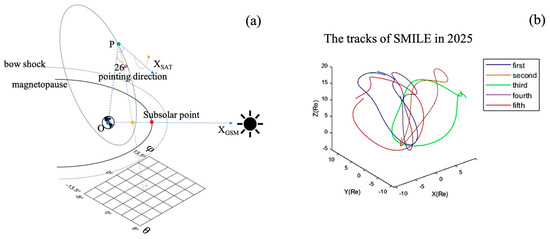
Figure 1.
Simulation of detection attitude during MHD imaging in satellite operation and selection of the tracks. (a) shows that the direction of the orientation is always the line between the satellite position and the center of the earth rotated by 26° around XSAT in the positive. The principle of MHD imaging is to integrate the 3D emission along the line of sight [10]. (b) The shape of every selected track under the GSM coordinate system in Table 1 (figure adapted from Wang et al. [16]).
The subsolar point is sometimes on the -axis. Then, the partial subsolar magnetopause can be imaged along the line of sight. The imaging integration method follows that of Sun et al. [15].
We used the simulated SMILE MHD images as the dataset considering that the satellite has not yet been launched (Figure 1b). The dataset of magnetospheric images is derived from simulated images of a hypothetical satellite on a candidate orbit of SMILE, with 1–5 satellite tracks in 2025 (Table 1). The sampling is performed every 3 min.

Table 1.
Satellite orbit times in 2025.
We selected 3D MHD X-ray emissions (the Lagrangian remapping MHD model developed by Hu et al. [28]) under seven sets of various solar wind parameters and interplanetary magnetic field (IMF) parameters (Table 2) to simulate the images. A direct calculation can justify that the X-ray intensity inside the magnetosphere is at least an order of magnitude smaller than that outside [5]. Therefore, for the value of the internal emissivity inside the magnetosphere, we set it to 0. Then, we filtered out the magnetopause images near the subsolar point followed by the UCFE-RF technique [16]. These images form the magnetopause dataset.
Table 2.
The parameters of the solar wind plasma and interplanetary magnetic field (IMF) BX, By, Bz.
The magnetopause dataset contains full and partial magnetopause shapes in the FOV, and the span of the magnetopause is greater than 5° on the -axis. The span of the magnetopause below 5° is considered so weak as to be unusable for TFA [16]. The magnetopause position can be masked in the image by defining the 3D magnetopause position. However, due to the unbalanced voxel resolution of the 3D MHD X-ray emissions with a minimum of 0.4Re, we cannot find the magnetopause location in the 3D model. In a way, if the satellite probes outside the magnetosphere (partly inside the magnetosheath) in the unlimited FOV, the whole magnetopause will appear [16]. Then, the magnetopause position is usually shown as the maximum value of the radiation at each angle at the -axis when the line of sight is tangent to the magnetopause [15]. So, magnetopause labels are obtained by expanding the view to reveal the whole magnetopause to find the maximum value of the radiation at each angle under the -axis.
Each image has an FOV of 16° 27° and the size is 161 271 under the resolution of 0.1°. The number of images is 17,064 in total. The partial dataset morphology is shown in Figure 2. These images contain the full and partial magnetopauses in the FOV, and the images correspond to different times, solar wind conditions, satellite positions (under the GSM coordinate system), and detection directions.
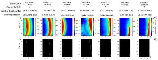
Figure 2.
Partial magnetopause morphology in the magnetopause dataset with different times (in Table 1) and solar wind conditions in Table 2. (a) The diverse magnetopause images under the SXI field of view (FOV) of 16° 27°. (b) The corresponding real magnetopause labels in (a). The first and second images in (a) have full magnetopause in the FOV.
3. Methods
3.1. Image Adaptive Preprocessing
The staple integral structure containing magnetopause (the white area of Figure 3b) can be obtained by pre-segmentation method from the images as a prior. From analyzing the characteristics of the image, there is a significant difference between the foreground (staple integral structure) and background (the others of the image). Nevertheless, OTSU threshold technology [29] is a nonparametric adaptive threshold selection for pre-segmenting the staple integral structure. The technology chooses an optimal threshold by discriminating to maximize the divisibility of the foreground and background at the gray level. Specifically, the gray values of an image are counted, after which a threshold is found to maximize the variance of the divided foreground and background. This technology is based on histogram statistics, without setting a threshold, but adaptively selecting a threshold to divide the foreground and background of the image. OTSU has a certain universality for all images. Therefore, we applied it to the magnetopause images.
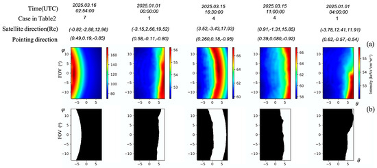
Figure 3.
OTSU threshold technique for expressing partial magnetopause datasets. (a) Part of the magnetopause dataset. (b) The corresponding preprocessed images followed the OTSU under (a). The white area is the staple integral structure (foreground). The black area is the other part of the image that acts as the background. Magnetopause is included in the structure.
3.2. Attention Block
3.2.1. Squeeze and Excitation Units
The squeeze and excitation (SE) network aims at informational dependencies between channels (Figure 4a). Channel feature response can be adaptively recalibrated by explicitly modeling the channel relevance [30]. The first step of the module is to squeeze each channel through an adaptive mean pooling operation to generate a global distribution of channel-level feature responses. An excitation operation follows. The excitation of each channel is controlled by sample-specific activations learned from the channel-dependent gating mechanism. The feature mappings are then reweighted to generate the output of the SE block [30]. This module improves the characterization of the network by enhancing the sensitivity of channel features in the local receptive field.
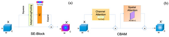
Figure 4.
The attention blocks. (a) The structure of SE block; (b) the structure of CBAM block.
3.2.2. Convolutional Block Attention Module
Convolutional Block Attention Module (CBAM) recalibrates strong feature correspondence in both spatial and channel dimensions by separately modeling channel and spatial dependencies [31]. It is a simple and effective attention module for feed-forward convolutional neural networks.
Each channel of the feature map is characterized by a feature detector [32]. First, the spatial information is aggregated using the average pooling method along the channel dimension [33]. Then, the maximum pooling gathers another important clue about features to infer more precise channel attention. Both average pooling and maximum pooling are used together to adapt to the strong feature correspondence of the channel. Afterwards, spatial attention is used after channel response, applying average pooling and maximum pooling operations along the channel axis, and concatenating them to generate the valid feature descriptor. It continues the channel attention sub-module and can effectively highlight areas of spatial information. Finally, the convolutional layer is added to generate the spatial attention sub-module [31].
CBAM generates the adaptive feature map from the feature responses of the two submodules (Figure 4b). It is a lightweight module that can be embedded into any network model to improve network performance.
3.3. Efficientnet as Encoder
We used the efficientnet network [34] as the encoder, with its main component being the mobile inverted bottleneck convolution (MBConv). Specifically, the MBConv module contains the deep separable convolution and drop connect from MobileNet [35]. Depth separable convolution includes depthwise and pointwise convolution. The MBConv module represents them separately, with the batch normalization layer (BN) and SE block added in between. Drop connect randomly sets the input weights of a hidden layer to zero, and the result is fed into the switch activation function. At the end of the module, the input of the module is added with the information processed by the series to get the output of the MBConv module. The structure of the module is shown in Figure 5a.
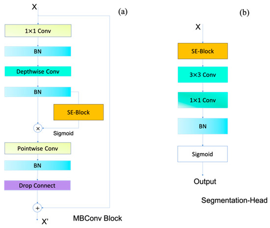
Figure 5.
The frameworks of the main blocks in the model. (a) The framework of the MBConv block. This is the foundation of the efficientnet. (b) The framework of the segmentation head.
Unlike the VGG, resnet, and densenet networks [36], the efficientnet backbone network considers the limitations of depth on performance. It takes into account the effects of depth, width, and resolution factors and combines them to form the series of efficientnet. We chose the efficientnet-b1 network [34] as the backbone, while the number of channels for each layer of outputs is (24, 40, 112, 320), and the number of MBConv basic modules used in each layer is (5, 3, 8, 7).
3.4. Loss Function
Using multi-scale loss to train models can fully optimize information from different scales in images, thereby improving the model’s ability to capture the target’s details and boundaries. Scale functions are often applied to multi-level semantic segmentation models to alleviate the long-tail problem of category imbalance, making the model more stable and convergent. The traditional loss function for semantic segmentation is cross-entropy loss. The binary cross-entropy (BCE) loss (2) is applied to the binary classification of foreground and background to calculate the entropy value.
BCELoss = −(y × log(p) + (1 − y) × log(1 − p))
For the magnetopause dataset, the pixel-level proportion of the magnetopause target in the image is 1:3 × 10², which leads to an imbalance in the ratio between the magnetopause and others of the image. When there are many easy samples (except magnetopause), the training of the model will be occupied by these. This will make it difficult to learn complex samples (magnetopause). Diceloss is a similarity measure loss function (3) aimed at finding the difference between two types of the samples. It mainly calculates the intersection information of two samples by multiplying the predicted values and real labels. Intersection calculation can effectively clear information in the predicted segmentation map that is not activated in the real labels, and learn complex samples with the small proportion of categories in the model.
We used the traditional BCE loss and diceloss to train the model (4). The multi-scale loss (L) catches complex magnetopause information in images that are difficult to extract. λ is set up to 0.5.
3.5. OESA-UNet Architecture
The overall architecture of the OESA-UNet is presented in Figure 6. We used the preprocessing image, SE block, CBAM, and efficientnet-b1 backbone to construct the model following the structure of the encoder and decoder. The OESA-UNet encoder uses the efficientnet backbone network to extract low-level semantic information. Nearest neighbor interpolation is applied to the first downsampling, and the convolutional operation is used at each downsampling after the first. The efficientnet-b1 backbone network can reduce the number of parameters for model training and improve training performance. After that, we inserted the CBAM module into the bottom feature to fuse the attention feature responses between the multi-dimensional channels and spaces. In the decoder structure, two SE blocks are put into each decoder layer. One is in the skip connection stage, and the other is before upsampling with the nearest interpolation. Two 3 3 convolutional layers are added between the two SE blocks. The segmentation head (Figure 5b) includes a 1 1 convolutional layer and batch normalization layer after the SE block. Sigmoid is the activation function. The inputs of the model are the preprocessed image and magnetosphere image. The features obtained by each encoder layer are connected to the corresponding decoder layer in a skipping manner, and we also connected depth features before the segmentation head and inputs.
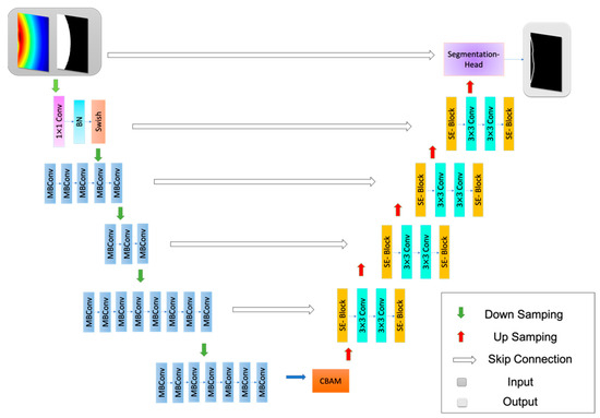
Figure 6.
The overview of the OESA-UNet, which is composed of the encoder (efficientnet network), decoder with attention block, and skip connection. Here, the CBAM block receives the last encoding feature.
4. Experiments and Metrics
4.1. Training
Our model used the Adam optimizer and had a learning rate of 0.1 in the first 25 epochs, 0.05 from 25 to 50 epochs, and 8 × 10⁻³ after 50 epochs, with a total number of 100 epochs and 32 batch sizes. We performed data augmentation on the training set, and randomly added noise to the data current inability to accurately simulate background pollution in the sky area during satellite operation. The ratio of the training set, validation set, and test set is 8:1:1. All experiments are implemented using NVIDIA RTX 2080 Ti and 16 GB of RAM. For training, we used pre-training weights on the advprop [37] for the encoder. The advprop technology can improve model performance by using adversarial samples from the imagenet dataset [38] for training. The pre-trained encoder under the efficientnet is insensitive to noisy datasets. We further trained our magnetosphere dataset followed by the weights.
4.2. Evaluation Metrics
Performance evaluation of segmentation is usually expressed in terms of pixel accuracy. For the issue of weak expression of the magnetopause in an image, we used recall, precision, and f1 score metrics to evaluate the quality of segmentation.
In addition, if an image can be exploited by TFA technology, it usually shows a larger proportion of the predicted magnetopause position and a smaller deviation compared to the truth. Finally, TFA technology can be used to invert the three-dimensional magnetopause position more accurately. We designed four indicators to evaluate the feasibility of being utilized by TFA.
The ratio of predicted magnetopause length (LP) under the truth (5) can represent how much magnetopause can be utilized by TFA. Lpre and Ltruth mean the predicted length of the magnetopause and the actual length, respectively.
Maximum angle deviation (6) and minimum angle deviation (7) metrics can obtain the deviation limit of the predicted magnetopause position. yi-pre and yi-truth represent the predicted and real position of the magnetopause at each i pixel under the axis.
The average angle deviation expresses the degree of stable divergence that TFA can utilize (8).
5. Results
We tried to segment our magnetopause using traditional image edge processing methods (e.g., Sobel, Laplacian, and Canny), and the results (Figure 7) found that most edge operators do not recognize specific magnetopause targets. Sobel and Laplacian can hardly recognize anything, and Canny’s weak segmentation result has a terrible error compared with the ground truth because there is no sudden change in gradient at the magnetopause. Therefore, these traditional edge processing methods have poor performance for specific targets under weak gradient changes.

Figure 7.
The results of the traditional edge operator with different times. The three-dimensional coordinates represent the satellite position and pointing direction of the SXI under the GSM coordinate system.
We compared our method with other semantic segmentation methods. The results show that recall, precision, and f1 score under the other networks do not reach 90% (Table 3), and these metrics are not balanced. The UNet series of networks works better. LinkNet [39] references the Unet structure and uses addition in the connection stage of encoder and decoder, performing better than the other methods in the last column of Figure 8c and less well in the second column. MAnet [40] has a large bias in the second column of Figure 8d. Meanwhile, Linknet and MAnet split the magnetopause line widely.
Table 3.
Results on comparing other segmentation networks.
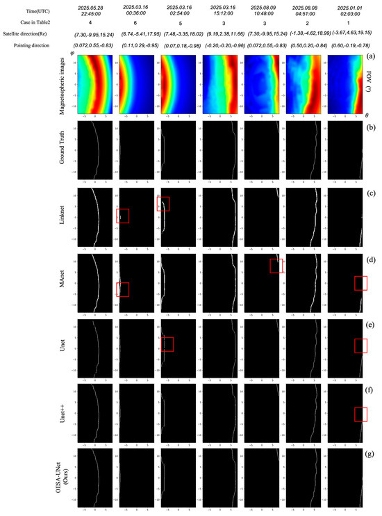
Figure 8.
Segmentation results using the different models. (a) For each case of magnetospheric images, (b) represents the true position of the magnetopause in the magnetospheric image. (c–g) are the segmentation result under the corresponding models. The red boxes indicate segmentation errors between the model and (b).
In our approach, we adjusted the encoder network and did ablation experiments. We compared the methods of changing the encoder backbone network, without adding the attention blocks, and without preprocessing the image.
In the experimental results of Table 4 (changing encoder backbone), vgg16, resnet50, and densenet backbone perform poorly. The Dpn68 network combines the resnet and densenet networks and thus outperforms our method in the precision metrics by 0.3%. Xception is a lightweight module that combines multi-scale information in the image. When used as the backbone network, it is only 0.1% higher in the recall metric than ours. However, ours performs better than others in the TFA evaluation metrics. Overall, the f1 score value of OXSA-UNet is slightly higher than that of ODPSA-UNet. From the segmentation results in Figure 9, the segmentation expression of ODPSA-UNet is not as good as that of OXSA-UNet. The various models perform well in the case where there is full magnetopause in the FOV, but there are deviations in the few cases where there are weak breaks in the magnetopause. For the last column in Figure 9c,d, there is a whole block that does not segment out in the small area, but ours can segment it out.
Table 4.
Comparative study on the changes of different encoder backbones.
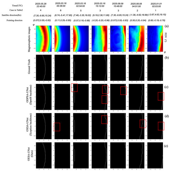
Figure 9.
Qualitative comparison of the different backbones. (a) For each case of magnetospheric images, (b) represents the true position of the magnetopause in the magnetospheric image. (c–e) are the segmentation result under the corresponding models. The red boxes indicate segmentation errors between the model and (b).
In the overall ablation study (Table 5), the OES-UNet model had the highest recall values and the OEA-UNet model had the highest display in precision values. The LP value performed well in OES-UNet, but the maximum angular deviation is large. Although there are errors in the performance of OES-UNet and OEA-UNet in the case of weak breaks (the third and fourth columns of Figure 10), it can segment out small blocks of the magnetopause in the small area (Figure 11c). Without CBAM, a longer arc curve can be obtained. Without SE, it has a weak arc curve. However, in the performance of Figure 11b and the first row of Figure 11a, not adding the CBAM module depresses the expression of magnetopause length. Not adding the SE module expands the length of the magnetopause. It misidentifies excess length. In the second row of Figure 11a, not adding the SE module cannot recognize the change of magnetopause, but without CBAM, the change is faint. The performance without the preprocessing effect is mediocre (Figure 10). Therefore, our model balances the influences of the modules without CBAM and SE. The enhancement effect is obvious after adding preprocessing, and the segmentation quality is better.
Table 5.
Ablation study w/o attention block and preprocessing.
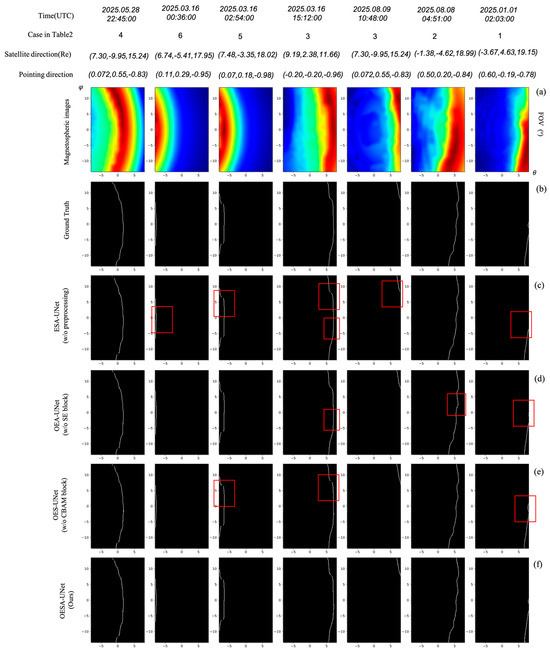
Figure 10.
Qualitative comparison of ablation study. (a) For each case of magnetospheric images, (b) represents the true position of the magnetopause in the magnetospheric image. (c–f) are the segmentation result under the corresponding models. The red boxes indicate segmentation errors between the model and (b).

Figure 11.
Magnified view of black-boxed patches predicted by different models. The three-dimensional coordinates represent the satellite position and pointing direction of the SXI under the GSM coordinate system. (a–c) Enlarged results of the black boxed areas in the corresponding magnetospheric images under the different cases.
All models have a minimum angular deviation value of 0. Under the mean angular deviation values, OXSA-UNet, OES-UNet, OEA-Unet, and ESA-UNet all reach the order of 1 × 10⁻³.
6. Discussion
In fact, for the image where the magnetopause is full in the FOV (such as the first column of Figure 10a), our model finds the magnetopause within 0.106 s. In contrast, the computational time to obtain the magnetopause by finding the maximum radiation value (MRV) in each row is 0.006 s. The running time of ours is 0.1 s slower than the MRV method, and there are a few biases in our model. However, the MRV method is not applicable when a partial magnetopause is present. There is no method to distinguish whether the acquired magnetospheric image is full magnetopause or not in the FOV. Our model can detect diverse magnetopause images under the limited FOV. Downstream tasks can be designed to classify the full magnetopause in the future.
The simulated image is ideal and does not contain cosmic and other noises. Real SMILE satellite images will contain noises from the instrument, the universe, and so on. Our model can incorporate noise processing and adversarial modules to overcome the impact of noises on future data.
We proposed OESA-UNet technology to detect the magnetopause position in images. Firstly, we preprocessed the images to segment the staple integral structure containing magnetopause. It can adaptively determine the region where the magnetopause is located.
7. Conclusions
Then, we used the efficientnet network as the encoder and the attention mechanism in the decoder following the U-shape structure. The fusion of low-level and high-level semantic features can finely identify the magnetospheric boundary. After that, a multi-scale loss is integrated to train the model, and the designed metrics can evaluate the feasibility of being utilized by TFA. The precision reaches 92.1%, recall reaches 93.8%, F1 score reaches 92.9%, and pixel accuracy reaches 99.9%. The average angle deviation can reach below 5 × 10⁻³ degrees, and the proportion of true length can reach over 0.97. The feasibility of being utilized by TFA technology is higher. The traditional detection method represents the position of the magnetopause by finding the maximum radiation value of each row in the image, but this only applies to the situation where the magnetopause is completely exposed at the φ axis. In the case where the magnetopause does not fully appear in the FOV, it is unable to find the magnetopause position. The advantage of our segmentation model is that it adapts to diverse magnetopause forms, which includes the shape accounting for more than 5° on the -axis. Even though we do not know if there is a full or partial magnetopause in a magnetospheric image that can be inverted by TFA due to the limitation of the current technology, we can use the OESA-UNet model. This adaptive detection model can quickly detect diverse magnetopause to serve TFA technology for three-dimensional magnetopause inversion and allow further study of the interaction between the magnetosphere on the Earth’s dayside and the solar wind.
Author Contributions
Conceptualization, D.L. and T.S.; methodology, J.W. and R.W.; code, J.W.; validation, J.W., R.W., D.L. and T.S.; investigation, J.W.; resources, T.S.; data curation, J.W. and R.W.; writing—original draft preparation, J.W.; writing—review and editing, J.W.; visualization, J.W.; supervision, D.L., T.S. and X.P. All authors have read and agreed to the published version of the manuscript.
Funding
This work was supported by the National Natural Science Foundation of China (Grant Nos. 42322408, 42188101, 42074202), Strategic Pioneer Program on Space Science, CAS, Grant Nos. XDA15350201, and XDA15014800.
Data Availability Statement
The data used for this study have been made available to the public in this ScienceDB repository link: https://doi.org/10.57760/sciencedb.07871 (accessed on 1 March 2024).
Acknowledgments
The authors gratefully acknowledge Y. Q. Hu for providing information on the MHD simulation code.
Conflicts of Interest
The authors declare no conflicts of interest.
References
- Cravens, T.E. Comet Hyakutake X-ray Source: Charge Transfer of Solar Wind Heavy Ions. Geophys. Res. Lett. 1997, 24, 105–108. [Google Scholar] [CrossRef]
- Bhardwaj, A.; Elsner, R.F.; Randall Gladstone, G.; Cravens, T.E.; Lisse, C.M.; Dennerl, K.; Branduardi-Raymont, G.; Wargelin, B.J.; Hunter Waite, J.; Robertson, I.; et al. X-rays from Solar System Objects. Planet. Space Sci. 2007, 55, 1135–1189. [Google Scholar] [CrossRef]
- Wang, C.; Sun, T. Methods to Derive the Magnetopause from Soft X-ray Images by the SMILE Mission. Geosci. Lett. 2022, 9, 30. [Google Scholar] [CrossRef]
- Branduardi-Raymont, G.; Wang, C.; Escoubet, C.P.; Sembay, S.; Donovan, E.; Dai, L.; Li, L.; Li, J.; Agnolon, D.; Raab, W.; et al. Imaging solar-terrestrial interactions on the global scale: The SMILE mission. In Proceedings of the EGU General Assembly Conference Abstracts, Online, 19–30 April 2021; p. EGU21-3230. [Google Scholar]
- Sun, T.R.; Wang, C.; Wei, F.; Sembay, S. X-ray Imaging of Kelvin-Helmholtz Waves at the Magnetopause. J. Geophys. Res. Space Phys. 2015, 120, 266–275. [Google Scholar] [CrossRef]
- Soman, M.R.; Hall, D.J.; Holland, A.D.; Burgon, R.; Buggey, T.; Skottfelt, J.; Sembay, S.; Drumm, P.; Thornhill, J.; Read, A.; et al. The SMILE Soft X-ray Imager (SXI) CCD Design and Development. J. Inst. 2018, 13, C01022. [Google Scholar] [CrossRef]
- Xu, Q.; Tang, B.; Sun, T.; Li, W.; Zhang, X.; Wei, F.; Guo, X.; Wang, C. Modeling of the Subsolar Magnetopause Motion Under Interplanetary Magnetic Field Southward Turning. Space Weather 2022, 20, 12. [Google Scholar] [CrossRef]
- Haaland, S.; Gjerloev, J. On the Relation between Asymmetries in the Ring Current and Magnetopause Current. JGR Space Phys. 2013, 118, 7593–7604. [Google Scholar] [CrossRef]
- Haaland, S.; Paschmann, G.; Øieroset, M.; Phan, T.; Hasegawa, H.; Fuselier, S.A.; Constantinescu, V.; Eriksson, S.; Trattner, K.J.; Fadanelli, S.; et al. Characteristics of the Flank Magnetopause: MMS Results. JGR Space Phys. 2020, 125, e2019JA027623. [Google Scholar] [CrossRef]
- Walsh, B.M.; Sibeck, D.G.; Nishimura, Y.; Angelopoulos, V. Statistical Analysis of the Plasmaspheric Plume at the Magnetopause. J. Geophys. Res. Space Phys. 2013, 118, 4844–4851. [Google Scholar] [CrossRef]
- Robertson, I.P.; Cravens, T.E. X-ray Emission from the Terrestrial Magnetosheath. Geophys. Res. Lett. 2003, 30, 2002GL016740. [Google Scholar] [CrossRef]
- Jorgensen, A.M.; Xu, R.; Sun, T.; Huang, Y.; Li, L.; Dai, L.; Wang, C. A Theoretical Study of the Tomographic Reconstruction of Magnetosheath X-ray Emissions. JGR Space Phys. 2022, 127, 4. [Google Scholar] [CrossRef]
- Collier, M.R.; Connor, H.K. Magnetopause Surface Reconstruction from Tangent Vector Observations. JGR Space Phys. 2018, 123, 12. [Google Scholar] [CrossRef]
- Jorgensen, A.M.; Sun, T.; Wang, C.; Dai, L.; Sembay, S.; Zheng, J.; Yu, X. Boundary Detection in Three Dimensions with Application to the SMILE Mission: The Effect of Model-Fitting Noise. J. Geophys. Res. Space Phys. 2019, 124, 4341–4355. [Google Scholar] [CrossRef]
- Sun, T.; Wang, C.; Connor, H.K.; Jorgensen, A.M.; Sembay, S. Deriving the Magnetopause Position from the Soft X-ray Image by Using the Tangent Fitting Approach. JGR Space Phys. 2020, 125, 9. [Google Scholar] [CrossRef]
- Wang, J.; Wang, R.; Li, D.; Sun, T.; Peng, X. An Approach of Filtering Simulated Magnetospheric X-ray Images Based on Self-Supervised Network and Random Forest. Phys. Scr. 2023, 98, 096002. [Google Scholar] [CrossRef]
- Kass, M.; Witkin, A.; Terzopoulos, D. Snakes: Active Contour Models. Int. J. Comput. Vis. 1988, 1, 321–331. [Google Scholar] [CrossRef]
- Burman, R.; Paul, S.; Das, S. A Differential Evolution Approach to Multi-Level Image Thresholding Using Type II Fuzzy Sets. In Swarm, Evolutionary, and Memetic Computing; Springer: Cham, Switzerland, 2013; pp. 274–285. [Google Scholar]
- Singh, S.; Singh, R. Comparison of Various Edge Detection Techniques. In Proceedings of the 2015 2nd International Conference on Computing for Sustainable Global Development (INDIACom), New Delhi, India, 11–13 March 2015; pp. 393–396. [Google Scholar]
- Xu, Q.; Ma, Z.; He, N.; Duan, W. DCSAU-Net: A Deeper and More Compact Split-Attention U-Net for Medical Image Segmentation. Comput. Biol. Med. 2023, 154, 106626. [Google Scholar] [CrossRef]
- Shinde, P.P.; Shah, S. A Review of Machine Learning and Deep Learning Applications. In Proceedings of the 2018 Fourth International Conference on Computing Communication Control and Automation (ICCUBEA), Pune, India, 16–18 August 2018; pp. 1–6. [Google Scholar]
- Zhu, X.; Cheng, Z.; Wang, S.; Chen, X.; Lu, G. Coronary Angiography Image Segmentation Based on PSPNet. Comput. Methods Programs Biomed. 2021, 200, 105897. [Google Scholar] [CrossRef]
- DeepLab: Semantic Image Segmentation with Deep Convolutional Nets, Atrous Convolution, and Fully Connected CRFs|IEEE Journals & Magazine|IEEE Xplore. Available online: https://ieeexplore.ieee.org/abstract/document/7913730 (accessed on 11 December 2023).
- Bi, L.; Feng, D.; Kim, J. Dual-Path Adversarial Learning for Fully Convolutional Network (FCN)-Based Medical Image Segmentation. Vis. Comput. 2018, 34, 1043–1052. [Google Scholar] [CrossRef]
- Khosravan, N.; Mortazi, A.; Wallace, M.; Bagci, U. PAN: Projective Adversarial Network for Medical Image Segmentation. In Medical Image Computing and Computer Assisted Intervention—MICCAI 2019; Springer: Cham, Switzerland, 2019; pp. 68–76. [Google Scholar]
- Jha, D.; Smedsrud, P.H.; Riegler, M.A.; Johansen, D.; Lange, T.D.; Halvorsen, P.D.; Johansen, H. ResUNet++: An Advanced Architecture for Medical Image Segmentation. In Proceedings of the 2019 IEEE International Symposium on Multimedia (ISM), San Diego, CA, USA, 9–11 December 2019; pp. 225–2255. [Google Scholar]
- Yu, W.; Yang, T.; Chen, C. Towards Resolving the Challenge of Long-Tail Distribution in UAV Images for Object Detection. In Proceedings of the 2021 IEEE Winter Conference on Applications of Computer Vision (WACV), Waikoloa, HI, USA, 3–8 January 2021; pp. 3257–3266. [Google Scholar]
- Hu, Y.Q.; Guo, X.C.; Wang, C. On the Ionospheric and Reconnection Potentials of the Earth: Results from Global MHD Simulations. J. Geophys. Res. Space Phys. 2007, 112, A07215. [Google Scholar] [CrossRef]
- Otsu, N. A Threshold Selection Method from Gray-Level Histograms. IEEE Trans. Syst. Man Cybern. 1979, 9, 62–66. [Google Scholar] [CrossRef]
- Hu, J.; Shen, L.; Sun, G. Squeeze-and-Excitation Networks. In Proceedings of the 2021 IEEE International Conference on Industrial Application of Artificial Intelligence (IAAI), Salt Lake City, UT, USA, 18–23 June 2018; pp. 7132–7141. [Google Scholar]
- Woo, S.; Park, J.; Lee, J.-Y.; Kweon, I.S. CBAM: Convolutional Block Attention Module. In Proceedings of the Computer Vision – ECCV 2018: 15th European Conference, Munich, Germany, 8–14 September 2018. [Google Scholar]
- Visualizing and Understanding Convolutional Networks|SpringerLink. Available online: https://www.usualwant.com/chapter/10.1007/978-3-319-10590-1_53 (accessed on 11 December 2023).
- Zhou, B.; Khosla, A.; Lapedriza, A.; Oliva, A.; Torralba, A. Learning Deep Features for Discriminative Localization. In Proceedings of the 2016 IEEE Conference on Computer Vision and Pattern Recognition (CVPR), Las Vegas, NV, USA, 27–30 June 2016; pp. 2921–2929. [Google Scholar]
- Tan, M.; Le, Q.V. EfficientNet: Rethinking Model Scaling for Convolutional Neural Networks. arXiv 2020, arXiv:1905.11946. [Google Scholar]
- Sandler, M.; Howard, A.; Zhu, M.; Zhmoginov, A.; Chen, L.-C. MobileNetV2: Inverted Residuals and Linear Bottlenecks; CRV: Leeuwarden, The Netherlands, 2018; pp. 4510–4520. [Google Scholar]
- Gikunda, P.K.; Jouandeau, N. State-of-the-Art Convolutional Neural Networks for Smart Farms: A Review. In Intelligent Computing; Arai, K., Bhatia, R., Kapoor, S., Eds.; Advances in Intelligent Systems and Computing; Springer International Publishing: Cham, Switzerland, 2019; Volume 997, pp. 763–775. ISBN 978-3-030-22870-5. [Google Scholar]
- Xie, C.; Tan, M.; Gong, B.; Wang, J.; Yuille, A.; Le, Q.V. Adversarial Examples Improve Image Recognition. arXiv 2020, arXiv:1911.09665. [Google Scholar]
- Deng, J.; Dong, W.; Socher, R.; Li, L.-J.; Li, K.; Li, F.-F. ImageNet: A Large-Scale Hierarchical Image Database. In Proceedings of the 2009 IEEE Conference on Computer Vision and Pattern Recognition, Miami, FL, USA, 20–25 June 2009; pp. 248–255. [Google Scholar]
- Chaurasia, A.; Culurciello, E. LinkNet: Exploiting Encoder Representations for Efficient Semantic Segmentation. In Proceedings of the 2017 IEEE Visual Communications and Image Processing (VCIP), St. Petersburg, FL, USA, 10–13 December 2017; pp. 1–4. [Google Scholar]
- He, P.; Jiao, L.; Shang, R.; Wang, S.; Liu, X.; Quan, D.; Yang, K.; Zhao, D. MANet: Multi-Scale Aware-Relation Network for Semantic Segmentation in Aerial Scenes. IEEE Trans. Geosci. Remote Sens. 2022, 60, 1–15. [Google Scholar] [CrossRef]
- Syazwany, N.S.; Nam, J.-H.; Lee, S.-C. MM-BiFPN: Multi-Modality Fusion Network With Bi-FPN for MRI Brain Tumor Segmentation. IEEE Access 2021, 9, 160708–160720. [Google Scholar] [CrossRef]
- Cao, H.; Wang, Y.; Chen, J.; Jiang, D.; Zhang, X.; Tian, Q.; Wang, M. Swin-Unet: Unet-like Pure Transformer for Medical Image Segmentation. arXiv 2021, arXiv:2105.05537. [Google Scholar]
Disclaimer/Publisher’s Note: The statements, opinions and data contained in all publications are solely those of the individual author(s) and contributor(s) and not of MDPI and/or the editor(s). MDPI and/or the editor(s) disclaim responsibility for any injury to people or property resulting from any ideas, methods, instructions or products referred to in the content. |
© 2024 by the authors. Licensee MDPI, Basel, Switzerland. This article is an open access article distributed under the terms and conditions of the Creative Commons Attribution (CC BY) license (https://creativecommons.org/licenses/by/4.0/).