InSAR-DEM Block Adjustment Model for Upcoming BIOMASS Mission: Considering Atmospheric Effects

Abstract

The unique P-band synthetic aperture radar (SAR) instrument, BIOMASS, is scheduled for launch in 2024. This satellite will enhance the estimation of subcanopy topography, owing to its strong penetration and fully polarimetric observation capability. In order to conduct global-scale mapping of the subcanopy topography, it is crucial to calibrate systematic errors of different strips through interferometric SAR (InSAR) DEM (digital elevation model) block adjustment. Furthermore, the BIOMASS mission will operate in repeat-pass interferometric mode, facing the atmospheric delay errors introduced by changes in atmospheric conditions. However, the existing block adjustment methods aim to calibrate systematic errors in bistatic mode, which can avoid possible errors from atmospheric effects through interferometry. Therefore, there is still a lack of systematic error calibration methods under the interference of atmospheric effects. To address this issue, we propose a block adjustment model considering atmospheric effects. Our model begins by employing the sub-aperture decomposition technique to form forward-looking and backward-looking interferograms, then multi-resolution weighted correlation analysis based on sub-aperture interferograms (SA-MRWCA) is utilized to detect atmospheric delay errors. Subsequently, the block adjustment model considering atmospheric effects can be established based on the SA-MRWCA. Finally, we use robust Helmert variance component estimation (RHVCE) to build the posterior stochastic model to improve parameter estimation accuracy. Due to the lack of spaceborne P-band data, this paper utilized L-band Advanced Land Observing Satellite (ALOS)-1 PALSAR data, which is also long-wavelength, to emulate systematic error calibration of the BIOMASS mission. We chose climatically diverse inland regions of Asia and the coastal regions of South America to assess the model’s effectiveness. The results show that the proposed block adjustment model considering atmospheric effects improved accuracy by 72.2% in the inland test site, with root mean square error (RMSE) decreasing from 10.85 m to 3.02 m. Moreover, the accuracy in the coastal test site improved by 80.2%, with RMSE decreasing from 16.19 m to 3.22 m.

1. Introduction

Interferometric synthetic aperture radar (InSAR) is a powerful tool for large-scale topographic mapping within remote sensing technologies due to its all-weather, all-day, and wide-area observation capability [1,2]. To further observe the three-dimensional structure of forests and estimate the subcanopy topography, the European Space Agency (ESA) proposed the BIOMASS mission [3], which has strong penetration capability due to operating in P-band. Compared with existing space-borne SAR satellites, BIOMASS holds excellent potential for global-scale inverting forest parameters [4] and estimating digital terrain models (DTMs) [5].

The BIOMASS mission will carry a P-band synthetic aperture radar (SAR) sensor with full polarimetric and tomographic capabilities, offering the first opportunity to measure global subcanopy topography [5]. The SAR will operate in repeat-pass interferometric mode and fly in a near-polar, Sun-synchronous orbit with a 637–666 km altitude. Due to instrument performance and high interferometric coherence requirements, the BIOMASS mission will achieve global coverage through interleave stripmap operations between three subswaths, which need a series of roll and repositioning maneuvers [5,6]. Therefore, the digital elevation models (DEMs) derived from BIOMASS will encounter systematic errors between different strips and atmospheric delay errors introduced by changes in atmospheric conditions [7,8,9]. To ensure the absolute height accuracy and the overall accuracy consistency of topography products, it is necessary to eliminate the above error sources.

For the systematic error calibration, one of the most effective methods is to establish the block adjustment model based on absolute elevation references from ground control points (GCPs) and elevation consistency constraints from tie-points (TPs) [10,11]. To achieve this, DLR (Microwaves and Radar Institute at the German Aerospace Center) utilized the spaceborne lidar, Ice, Cloud, and land Elevation Satellite-1 (ICESat-1) [12] as GCPs and proposed block adjustment using a two-dimensional polynomial as the function model [1,9,10,11], which generated global topography products TanDEM-X DEM. As the successor to ICESat-1, ICESat-2 offers GCPs with higher spatial resolution and higher repetition rates [13]. Due to the distribution and accuracy of GCPs and ensuring height matching being the keys for systematic error calibration [14,15], researchers began using ICESat-2 as GCPs and considered horizontal errors of DEMs, further improving the block adjustment methods [16,17]. However, the existing block adjustment methods aim to calibrate systematic errors in bistatic mode, whose atmospheric effects can be effectively eliminated through interferometry [18]. Therefore, for the BIOMASS mission, there is an urgent need for a systematic error calibration algorithm under the interference of atmospheric effects. In addition, for the P-band, the atmospheric delay errors significantly affect the elevation accuracy of DEM [7]. Moreover, it also interferes with the height matching between DEMs and GCPs, as well as between TPs, thus affecting the calibration of systematic errors. However, the existing atmospheric effects correction methods usually rely on external water vapor data [19] or require extensive SAR data to perform spatiotemporal analyses [20], limiting the real-time correction of atmospheric effects on a global scale.

Given the above issue, we utilize ICESat-2 ATL08 data as GCPs and propose the block adjustment model considering atmospheric effects for the BIOMASS mission. First, we use the block adjustment model to weaken atmospheric effects’ interference in estimating systematic errors. Second, the forward-looking interferograms (F-Infs) and backward-looking interferograms (B-Infs) are composed by sub-aperture decomposition [21]. Then, the atmospheric delay errors can be detected through the multi-resolution weighted correlation analysis based on sub-aperture interferograms (SA-MRWCA), which can correct atmospheric effects without relying on external water vapor data. Finally, we establish the block adjustment model considering atmospheric effects and utilize robust Helmert variance component estimation (RHVCE) [22] to determine weight ratios for GCPs and TPs, overcoming the interference of gross errors and achieving fine systematic error calibration.

2. Methodology

InSAR-DEM block adjustment aims to calibrate systematic errors in different strips to fulfill height accuracy requirements and accomplish large-scale topographic mapping [9,23]. However, due to the error equation’s lack of consideration for atmospheric delay errors’ impact on height matching, current block adjustment methods prove inadequate for estimating systematic errors in repeat-pass interferometric mode. Hence, this section mainly describes the proposed block adjustment model considering atmospheric effects to address this issue.

2.1. InSAR-DEM Block Adjustment Based on Function Model

The interference factors such as baseline inaccuracies, random phase errors, and radar instruments residual offsets can cause residual systematic errors in different strips [10,11]. The above error sources primarily include offsets and tilts in range and azimuth, which can typically be modeled using a two-dimensional polynomial about image coordinates:

$$g_i\left(x,y\right)=a_i+b_{i}x+c_{i}y+d_{i}xy+e_i{x}^2+f_i{y}^2$$

(1)

where $i$ is the index of the DEM acquisition, $g_i(x,y)$ is the height error function, and $x,y$ are the range and azimuth coordinates. $\left\{a_i,b_i,c_i,d_i,e_i,f_i\right\}$ are the unknown error parameters of the block adjustment model, which can be estimated using height constraints from GCPs and height consistency constraints from TPs.

For the bistatic mode, since the atmospheric conditions of the two SAR images are the same, the atmospheric delay errors can be eliminated through interferometry [1]. Therefore, the error equations of block adjustment are as follows:

$$\left\{\begin{array}{c}{\mathit{V}}_{GCP}={\mathit{H}}_{GCP}-\left({\widehat{\mathit{H}}}_i+g_i\left(x,y\right)\right)\\ {\mathit{V}}_{TP}=-\left({\widehat{\mathit{H}}}_j+g_j\left(x,y\right)\right)+\left({\widehat{\mathit{H}}}_k+g_k\left(x,y\right)\right)\end{array}\right.$$

(2)

where ${\mathit{V}}_{GCP}$ and ${\mathit{V}}_{TP}$ are residual vectors of GCPs and TPs, respectively. ${\mathit{H}}_{GCP}$ is the height of GCPs, and $\widehat{\mathit{H}}$ is the initial height matched on InSAR-DEM. $j$ and $k$ are the indices of adjacent and overlapping DEMs. Then, we can use the least squares principle to calculate the unknown error parameters and correct the systematic errors in each DEM:

$$\left\{\begin{array}{c}\left|{\mathit{V}}^T\mathit{P}\mathit{V}\right|=min\\ \begin{array}{cc}\mathit{V}={\left[\begin{array}{cc}{\mathit{V}}_{GCP}& {\mathit{V}}_{TP}\end{array}\right]}^T& \mathit{P}=\left[\begin{array}{cc}{\mathit{P}}_{\mathit{G}\mathit{C}\mathit{P}}& 0\\ 0& {\mathit{P}}_{TP}\end{array}\right]\end{array}\\ {DEM}_{post-adjust}^i\left(x,y\right)={DEM}_{pre-adjust}^i\left(x,y\right)+g_i\left(x,y\right)\end{array}\right.$$

(3)

where $T$ denotes the vector transposition, $\mathit{V}$ is the residual matrix, and $\mathit{P}$ is the stochastic model that characterizes the weight of observation equations in Equation (2).

2.2. Atmospheric Effects Correction Based on Correlation Analysis

Due to different atmospheric conditions in the repeat-pass interferometric mode, the propagation path and propagation speed of SAR ranging signals will change in the atmosphere, introducing atmospheric delay errors in InSAR-DEM [20,24]. Therefore, the core factors affecting DEM accuracy are systematic errors and atmospheric delay errors [24,25]. At this point, the height matching of the error equations shown in Equation (2) will be disturbed, which should transform into

$$\left\{\begin{array}{c}{\mathit{V}}_{GCP}={\mathit{H}}_{GCP}-\left({\widehat{\mathit{H}}}_i+{∆\mathit{H}}_i+g_i\left(x,y\right)\right)\\ {\mathit{V}}_{TP}=-\left({\widehat{\mathit{H}}}_j+{∆\mathit{H}}_j+g_j\left(x,y\right)\right)+\left({\widehat{\mathit{H}}}_k+{∆\mathit{H}}_k+g_k\left(x,y\right)\right)\end{array}\right.$$

(4)

where $∆\mathit{H}$ represents atmospheric delay errors. A lightweight atmospheric effects correction method is urgently needed to estimate systematic errors accurately through block adjustment.

In the atmosphere, the troposphere and ionosphere severely impact SAR signals, resulting in troposphere delay errors and ionospheric delay errors in InSAR-DEM [26]. Among them, the troposphere mainly causes the delay of the SAR signal propagation path, which is manifested as the tropospheric delay phase ${\phi }_{trop}$ in the InSAR interferogram [24,26]:

$${\phi }_{trop}=\frac{4\pi }{\lambda }\frac{{10}^{-6}}{\cos \theta }{\int }_z^{z_{top}}Ndl$$

(5)

where $\lambda$ is the wavelength, $\theta$ is the SAR incidence angle, $N$ is the zenith total delay, and $z$ and $z_{top}$ represent the surface elevation and tropospheric elevation, respectively. Under identical tropospheric conditions, shorter wavelengths reduce penetration into the troposphere and increase range delay. Therefore, long-wavelength SAR data can resist the interference of tropospheric delay for InSAR deformation measurements. However, for InSAR terrain mapping, the wavelength λ will be eliminated when the tropospheric delay phase ${\phi }_{trop}$ undergoes phase-to-height conversion, as shown in Equation (6). So, the tropospheric delay errors ${\sigma }_{trop}$ are independent of wavelength $\lambda$.

$$\left\{\begin{array}{c}{k}_z=\frac{4\pi B_{\perp }}{\lambda R\sin \theta }\\ {\sigma }_{trop}=\frac{{\phi }_{trop}}{k_z}\end{array}\right.$$

(6)

where $k_z$ is the phase-to-height conversion factor determined by the baseline parameters, $B_{\perp }$ is the vertical baseline, $R$ is the slant-range, and ${\sigma }_{tropo}$ is the tropospheric delay errors after phase-to-height conversion. In particular, although BIOMASS will operate in a Sun-synchronous orbit to mitigate the effects of ionosphere disturbances, all measurements will still be influenced by the ionosphere [7]. The main impacts include Faraday rotation $\mathsf{\Omega }$ and range delay ${\phi }_{iono}$:

$$\left\{\begin{array}{c}\mathrm{\Omega }=\frac{K}{f^2}〈B·\cos \psi 〉·\sec \theta ·TEC\\ {\phi }_{iono}=2\pi \frac{K}{cf}·TEC\end{array}\right.$$

(7)

where constant $K=40.28 {\mathrm{m}}^3/{\mathrm{s}}^2$, $f$ is the wave frequency, $B$ is the magnetic field, $\psi$ is the magnetic declination, and $TEC$ is the Total Electron Content (TEC). Under identical ionospheric conditions, the longer the wavelength of the SAR signal, the more serious the ionospheric delay will be.

In summary, considering the needs of BIOMASS global terrain mapping, atmospheric correction is crucial. Liu et al. proposed the multi-resolution weighted correlation analysis (MRWCA) method, achieving atmospheric effects correction of single-baseline dual-polarization SAR data without external water vapor data [24]. To further alleviate the limitations imposed by the polarization mode, we propose the SA-MRWCA method for single-baseline single-polarization SAR data. Specifically, the SAR images are divided into F-Infs and B-Infs under different squint angles using sub-aperture decomposition. Based on the independence assumption between atmospheric effects and squint angles, the SA-MRWCA can detect similar atmospheric delay errors in sub-aperture interferograms. Although the sub-aperture decomposition changes the overall information characteristics of the interferograms, the atmospheric effects are hardly affected, manifesting the same attributes in the sub-aperture interferograms. This provides the possibility to detect the atmospheric delay phase (ADP) [21]. For stable ground scattering targets, the main components of the interferometric phase ${\phi }_{int}$ include

$${\phi }_{int}={\phi }_{flat}+{\phi }_{topo}+{\phi }_{orb}+{\phi }_{atm}+{\phi }_{noi}$$

(8)

where ${\phi }_{flat}$ is the flat-earth phase, ${\phi }_{topo}$ is the topographic phase, ${\phi }_{orb}$ is the orbit error phase caused by the inaccuracy of orbit parameters, ${\phi }_{atm}$ is the ADP, and ${\phi }_{noi}$ is the noise phase (NP). After the sub-aperture decomposition, the forward- and backward-looking interferometric phases ${\phi }_{int}^{F/B}$ can be represented as

$${\phi }_{int}^{F/B}={\phi }_{flat}^{F/B}+{\phi }_{topo}^{F/B}+{\phi }_{orb}^{F/B}+{\phi }_{atm}^{F/B}+{\phi }_{noi}^{F/B}$$

(9)

where $F/B$ represents forward- and backward-looking, respectively. Among the phase components shown in Equations (8) and (9), ${\phi }_{flat}$ is the systematic phase contributed by the reference ellipsoidal surface, and ${\phi }_{orb}$ is only related to the orbit parameters of SAR satellites, so they are the same in F-Infs and B-Infs. Additionally, the partial phase associated with the scattering characteristics of the ground target in ${\phi }_{topo}$ will be slightly different between F-Infs and B-Infs. At the same time, ${\phi }_{noi}$ will show randomness in sub-aperture interferograms. Most importantly, the changes in atmospheric conditions between F-Infs and B-Infs are insignificant compared with the distance from the satellite to the ground scattering target. Therefore, ${\phi }_{atm}$ is almost the same in F-Infs and B-Infs.

The SA-MRWCA is based on the MRWCA for multi-resolution analysis of F-Infs and B-Infs through wavelet transform [24], utilizing correlation analysis to estimate atmospheric effects, which requires that ADP is the only similar signal in the phase components. Therefore, the other identical or similar phase components must be eliminated. To achieve this purpose, we first employ SRTM DEM [2], generated based on InSAR, and ASTER GDEM [27], generated based on optical stereophotogrammetry, to perform differential interferometry of F-Infs and B-Infs:

$${\phi }_{int}^{F/B}={\phi }_{\epsilon topo}^{F/B}+{\phi }_{orb}^{F/B}+{\phi }_{atm}^{F/B}+{\phi }_{noi}^{F/B}$$

(10)

where ${\phi }_{\epsilon topo}^{F/B}$ represents the topographic error phase (TEP). Due to the different error sources of the above two DEMs, ${\phi }_{\epsilon topo}^F$ and ${\phi }_{\epsilon topo}^B$ are also different in forward-looking differential interferograms (F-DInfs) and backward-looking differential interferograms (B-DInfs). Subsequently, the same orbit error phase ${\phi }_{orb}$ can be removed through polynomial fitting [28] or block adjustment:

$${\phi }_{int}^{F/B}={\phi }_{\epsilon topo}^{F/B}+{\phi }_{atm}^{F/B}+{\phi }_{noi}^{F/B}$$

(11)

At this point, the ADP is the only similar phase component between F-DInfs and B-DInfs. Moreover, the TEP and the NP primarily consist of high-frequency signals in the frequency domain, while the ADP predominantly includes low-frequency signals. Based on the differences in frequency characteristics, the SA-MRWCA decomposes F-DInfs and B-DInfs into building blocks through forward wavelet transform [24]. Then, it utilizes the weighted correlation analysis to estimate the wavelet coefficients associated with the ADP. Finally, the ADP is reconstructed by refining the wavelet coefficients in the inverse wavelet transform process to achieve the estimation of atmospheric delay errors. By substituting the atmospheric delay errors into the error equations shown in Equation (4), height matching between DEMs and GCPs, as well as between TPs, can be achieved for the repeat-pass interferometric mode of BIOMASS.

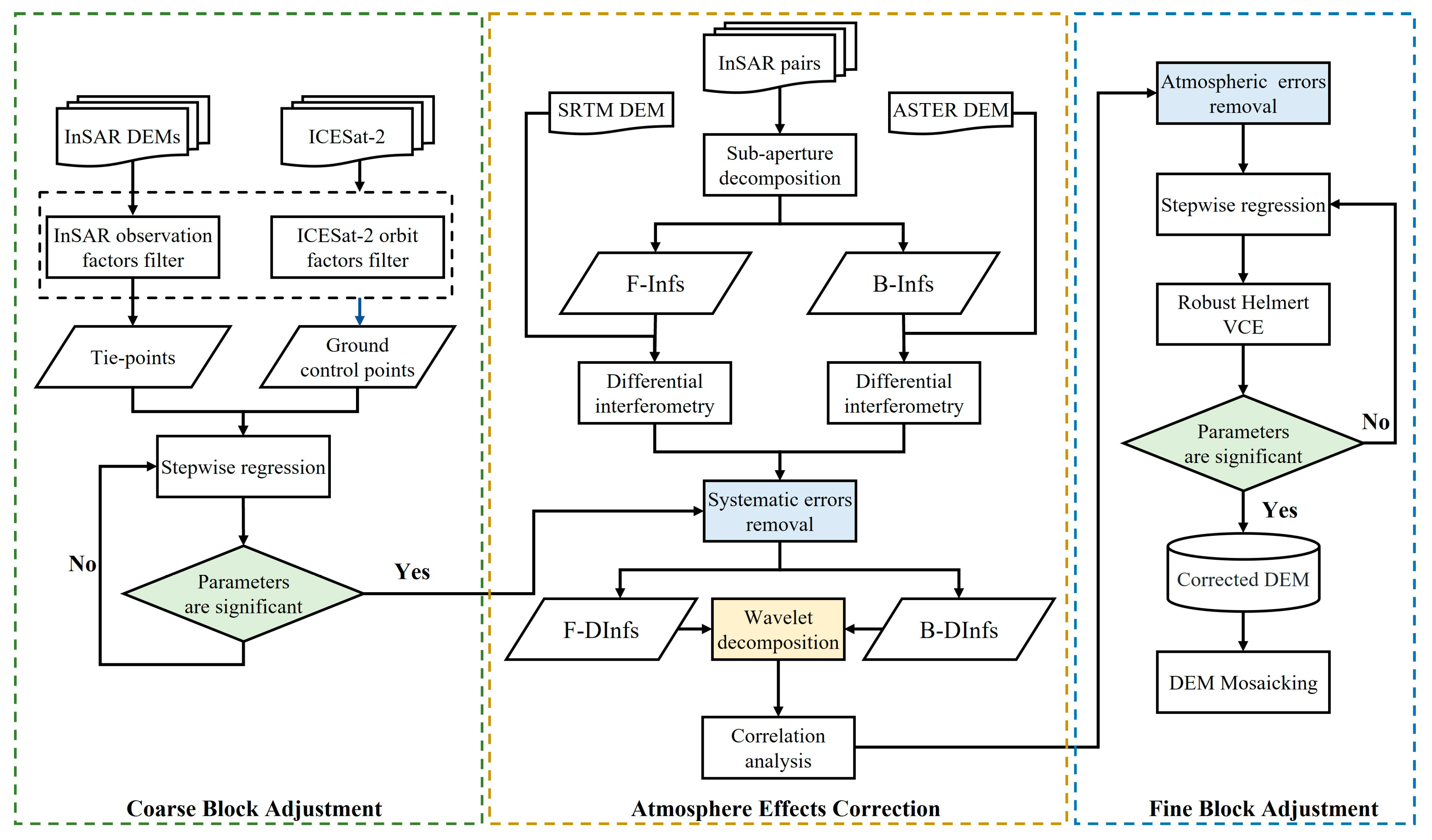
2.3. InSAR-DEM Block Adjustment Model Considering Atmospheric Effects

Based on the above analysis, we can establish the block adjustment model considering atmospheric effects to calibrate systematic errors under the interference of atmospheric delay errors. Figure 1 shows that the algorithm mainly includes the following three stages.

(1)

Coarse Block Adjustment

The core task of this stage involves selecting GCPs and TPs and then utilizing the block adjustment model, as shown in Equations (1)–(3), to provide the orbit error phase ${\phi }_{orb}$ for atmospheric effects correction. Compared with fitting the orbit error phase ${\phi }_{orb}$ scene by scene, this method uses the overall observations of the block adjustment as constraints, weakening the interference of the ADP on the polynomial fitting orbit error phase ${\phi }_{orb}$, thus separating the two as much as possible. High-quality GCPs and TPs are needed to achieve this goal [14,15], with the selection criteria shown in

Table 1. Selection criteria for Ground control points (GCPs) and tie-points (TPs).

	Data Sources	Chip Grid	Selection Criteria
GCPs	ICESat-2 ATL08 Version 5	5 km × 5 km	1. Strong beam 2. Cloud cover less than 20% 3. Not located in the geometric distortion area of SAR images 4. InSAR coherence greater than 0.5
TPs	InSAR DEMs	3 km × 3 km	1. Slope less than 30° 2. Not located in the geometric distortion area of SAR images 3. InSAR coherence greater than 0.5

.

We use ICESat-2 ATL08 (Version 5) data [13] as GCPs and divide the overlapping DEMs uniformly into 3 km × 3 km grids, with the central points selected as TPs. Then, we integrate the ICESat-2 orbit, InSAR observations, and terrain factors as the selection criteria to refine the GCPs and TPs. The selection criteria determine the quality of the GCPs and TPs, playing a crucial role in DEM calibration. To further improve the quality of points and reduce the interference of atmospheric delay errors on height matching, a reselection based on the 3-sigma rule is carried out:

$$\left\{\begin{array}{c}abs\left(H_{GCP}-H_{TanDEM-X DEM}\right)<3*{\sigma }_{H_{GCP}-H_{TanDEM-X DEM}}\\ abs\left(H_{GCP}-H_{InSAR-DEM}\right)<3*{\sigma }_{H_{GCP}-H_{InSAR-DEM}}\\ abs\left(H_{TIE\_j}-H_{TIE\_k}\right)<3*{\sigma }_{H_{TIE\_j}-H_{TIE\_k}}\end{array}\right.$$

(12)

where $H_{GCP}$, $H_{TanDEM-XDEM}$, and $H_{InSAR-DEM}$ represent the height of GCPs, TanDEM-X DEM, and InSAR-DEM, respectively. $H_{TIE\_j}$ and $H_{TIE\_k}$ represent the height of adjacent and overlapping DEMs. Then, we downsample the GCPs using a 5 km × 5 km grid and select the GCPs with the smallest elevation uncertainty [13] within each grid as the GCP used for block adjustment. The remaining parts will serve as checkpoints after block adjustment.

By using the selected GCPs and TPs, we can establish the error equations shown in Equation (2). Then, the unknown parameters of the block adjustment model can be estimated by utilizing the least-squares principle iteratively to realize the adaptive correction of systematic errors by the function model [11]:

$$t=\frac{{\widehat{x}}_{est}}{{\sigma }_{{\widehat{x}}_{est}}}$$

(13)

where ${\widehat{x}}_{est}$ and ${\sigma }_{{\widehat{x}}_{est}}$ represent the unknown parameters and their standard deviation, respectively. If the significance of all parameters $t\ge 1.64$, then accept all parameters. Otherwise, iterate the estimation by reducing one parameter at a time until all remaining parameters are significant [11]. As shown in Figure 1, the systematic errors based on coarse block adjustment serve as the orbit error phase in atmospheric effect correction, making the ADP the only similar phase component in Equation (11).

(2)

Atmosphere Effects Correction

Previous studies have reported that the ionosphere delay errors usually show a similar trend to the orbit error phase, causing the traditional polynomial fitting method to correct the orbit error to fail [29]. However, with the help of the systematic error estimated by the coarse block adjustment, the orbit error phase and the ADP in F-DInfs and B-DInfs can be more accurately separated. After removing the orbit error phase, the ADP is the only similar phase component between F-DInfs and B-DInfs, which can be detected through the SA-MRWCA, providing a basis for block adjustment considering atmospheric effects.

(3)

Fine Block Adjustment

As shown in Figure 1, unlike the coarse block adjustment, the fine block adjustment utilizes the atmospheric delay errors detected by the SA-MRWCA to establish the error equations considering atmospheric effects, achieving height matching for the block adjustment of repeat-pass interferometric mode. Furthermore, since the GCPs and TPs come from two different observation systems, the priori stochastic model $\mathit{P}$ in Equation (3) may not be appropriate, and the error equations shown in Equation (4) is also susceptible to interference from gross error. Therefore, after realizing systematic error adaptation through a t-test, we use RHVCE [22] in fine block adjustment to calculate the robust posterior stochastic model. In this way, the weight ratio of GCPs and TPs can be adjusted while overcoming the interference of gross errors. Combining the systematic errors estimated from block adjustment and the atmospheric delay errors detected by the SA-MRWCA, we can conduct precise error calibration:

$$\left\{\begin{array}{c}\left|{\mathit{V}}^T{\mathit{P}}_{RHVCE}\mathit{V}\right|=min\\ {DEM}_{post-adjust}^i\left(x,y\right)={DEM}_{pre-adjust}^i\left(x,y\right)+g_{RHVCE}^i\left(x,y\right)+{∆H}_{atm}(x,y)\end{array}\right.$$

(14)

where ${\mathit{P}}_{RHVCE}$ represents the robust posterior stochastic model estimated by RHVCE, $g_{RHVCE}^i\left(x,y\right)$ represents the systematic errors estimated based on ${\mathit{P}}_{RHVCE}$, and ${∆H}_{atm}(x,y)$ represents the atmospheric delay errors estimated by the SA-MRWCA at position $(x,y)$.

3. Test Sites and Data Sets

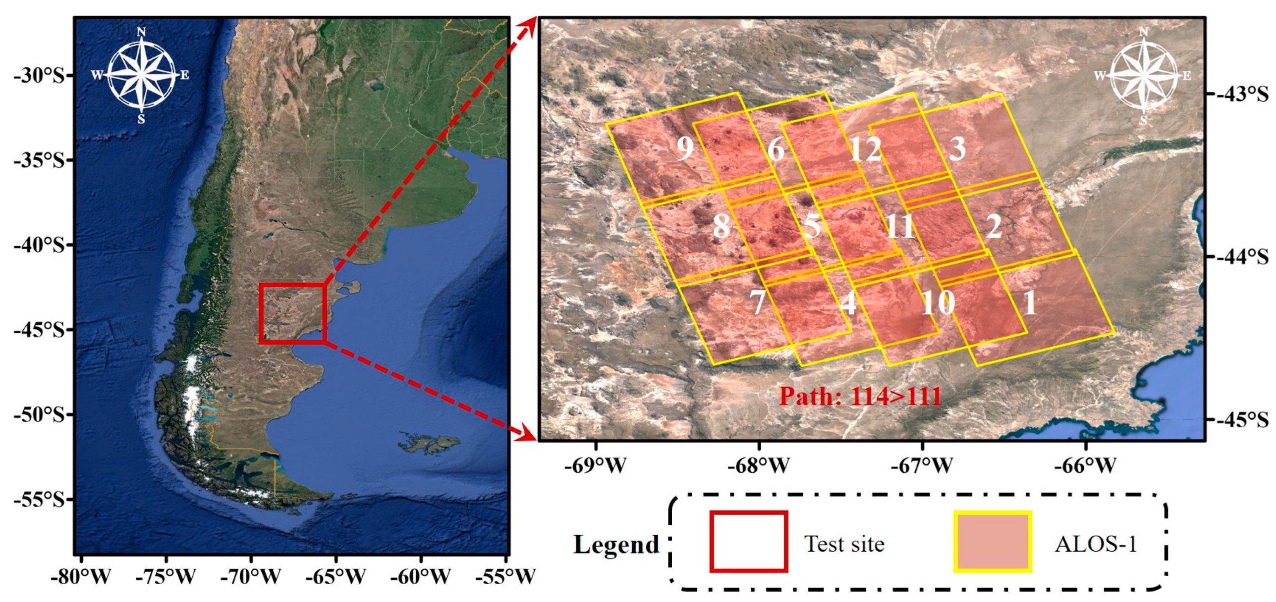
To fully verify the algorithm’s effectiveness, we conducted experiments in inland regions of Asia and coastal regions of South America with significant climate differences. Due to the lack of spaceborne P-band InSAR data, we emulated the BIOMASS data through L-band Advanced Land Observing Satellite (ALOS)-1 PALSAR data [30], which was also long-wavelength.

3.1. Test Sites

3.1.1. Inland Test Site

As shown in Figure 2, the inland test site lies at the junction of China and Mongolia. Situated in the midlatitude region of inland Asia. The test site exhibits a typical temperate continental climate: hot summers, cold winters, little precipitation, low air humidity, and a relatively stable atmosphere. In addition, hills and mountains dominate the topography of the area.

3.1.2. Coastal Test Site

Unlike the stable atmosphere in the inland test site, as shown in Figure 3, the coastal test site lies in South America’s midlatitude eastern coastal area, facing the Atlantic Ocean to the east. The ocean brings a humid climate and an active atmosphere. Additionally, hills and plains dominate the test site.

3.2. Data Sets

3.2.1. ALOS-1 PALSAR

In 2006, the Japan Aerospace Exploration Agency (JAXA) launched the ALOS-1 satellite carrying the L-band PALSAR for research in Earth resource survey, environmental monitoring, and natural disaster management [30]. ALOS-1 has a 46-day repeat cycle and features multiple polarization and multimode capabilities. We used HH-polarization data from fine-beam dual-polarization (FBD) mode to emulate block adjustment considering atmospheric effects for the BIOMASS mission.

Table 2. The information of ALOS-1 PALSAR data used in this study.

Test Sites	Time	Number *	Path *	$\overline{\mathbf{B}}\mathbf{p}\mathbf{e}\mathbf{r}\mathbf{p}$(m)	$\mathbf{B}\mathbf{t}\mathbf{e}\mathbf{m}\mathbf{p}$	Pixel Spacing (m)	Orbit
Inland	25 July 2010	1–3	482	557.5	92	3.16 × 9.37	ASC
	11 August 2010	4–6	483	435.6	46	3.16 × 9.37	ASC
	28 August 2010	7–9	484	317.3	46	3.16 × 9.37	ASC
	14 September 2010	10–12	485	465.3	46	3.16 × 9.37	ASC
Coastal	4 June 2010	1–3	111	131.4	46	3.26 × 9.37	ASC
	8 July 2010	4–6	113	160.9	46	3.26 × 9.37	ASC
	25 July 2010	7–9	114	537.5	46	3.26 × 9.37	ASC
	6 August 2010	10–12	112	489.3	46	3.26 × 9.37	ASC

“*” indicates correspondence to Figure 1 and Figure 2.

shows the data information in the inland and coastal test sites.

3.2.2. ICESat-2 ATL08 Product (Version 5)

The National Aeronautics and Space Administration (NASA) has released the fifth version of the land elevation product ATL08 through photon cloud filtering and classification of ICESat-2 ATL03 data [13]. The ATL08 data provide terrain and canopy heights at a 20 m along-track spacing, which has been widely used for DEM systematic error correction or forest height deduction [16,31]. In actual quality assessments, the accuracy of ATL08 terrain elevation can reach 0.73 m [32]. Previous studies have shown that the quality of GCPs is crucial for block adjustment [14,15]. To ensure the reliability of GCPs, we established extraction rules and refined ATL08 data within the two test sites from 14 October 2018 to 15 July 2021, as shown in Table 1.

3.2.3. Global Digital Elevation Products

We introduced the SRTM DEM and ASTER GDEM to remove the topographic phases of F-Infs and B-Infs, respectively. In addition, the higher-precision TanDEM-X DEM was utilized to verify the correction of atmospheric delay errors and systematic errors in continuous space.

Table 3. The information of the DEMs used in this study.

Dataset	Horizontal Datum	Vertical Datum	Time (Year)	Resolution (m)	Absolute Vertical Accuracy (m)	Technique
TanDEM-X DEM	WGS84	WGS84	2016	30	10	InSAR
SRTM DEM V003	WGS84	EGM96	2013	30	16	InSAR
ASTER GDEM V2	WGS84	EGM96	2011	30	17	Optical stereophotogrammetry

shows the information of the above DEMs. Before using the SRTM DEM and ASTER GDEM, it is necessary to convert their vertical datum to WGS84.

4. Results and Analysis

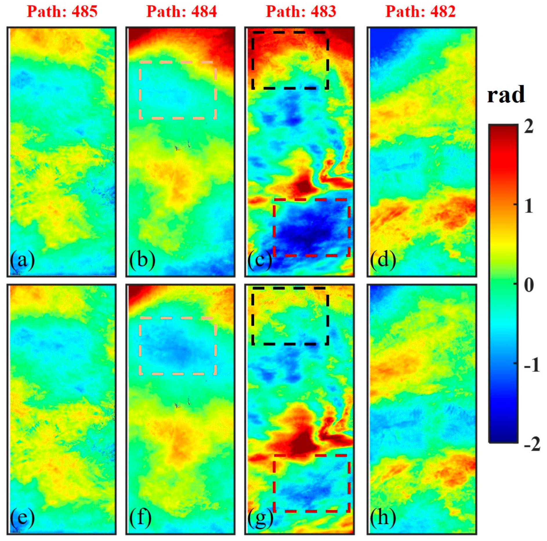
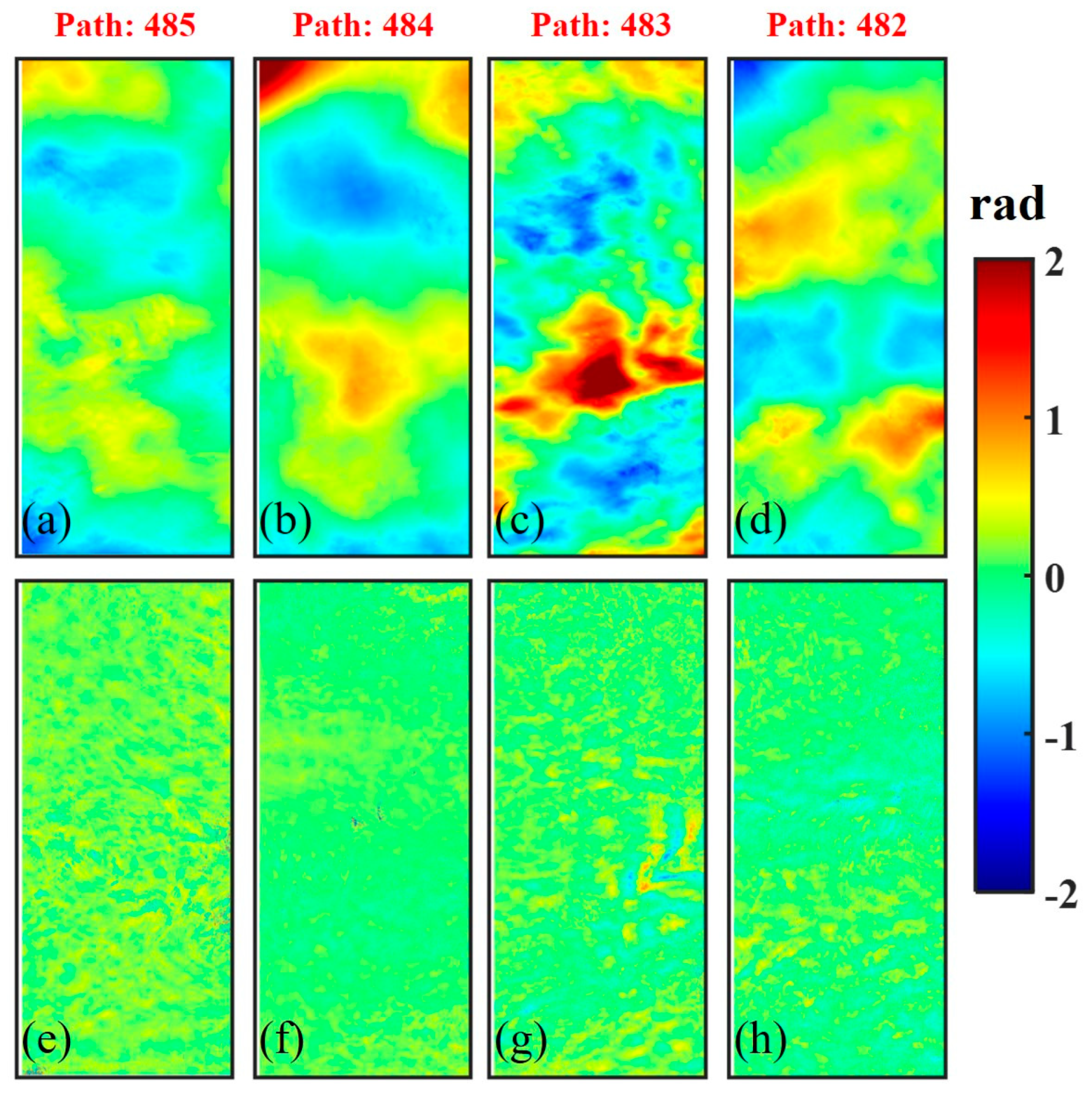
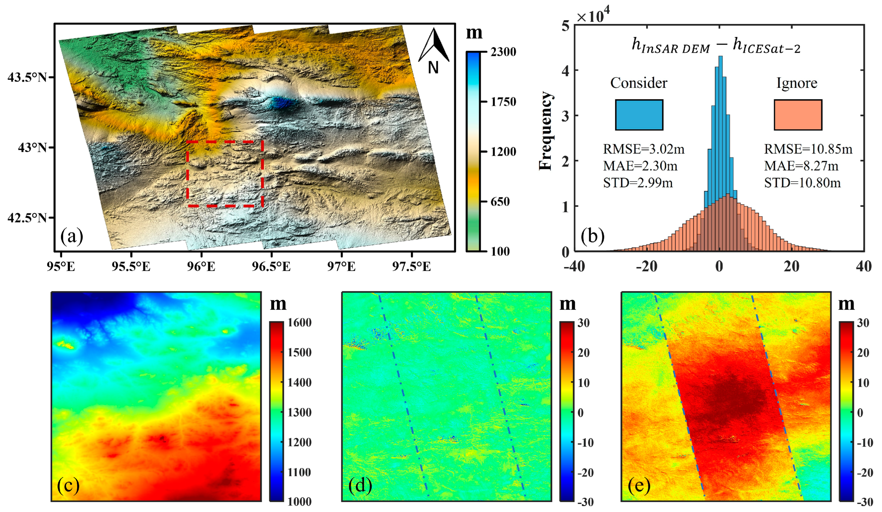
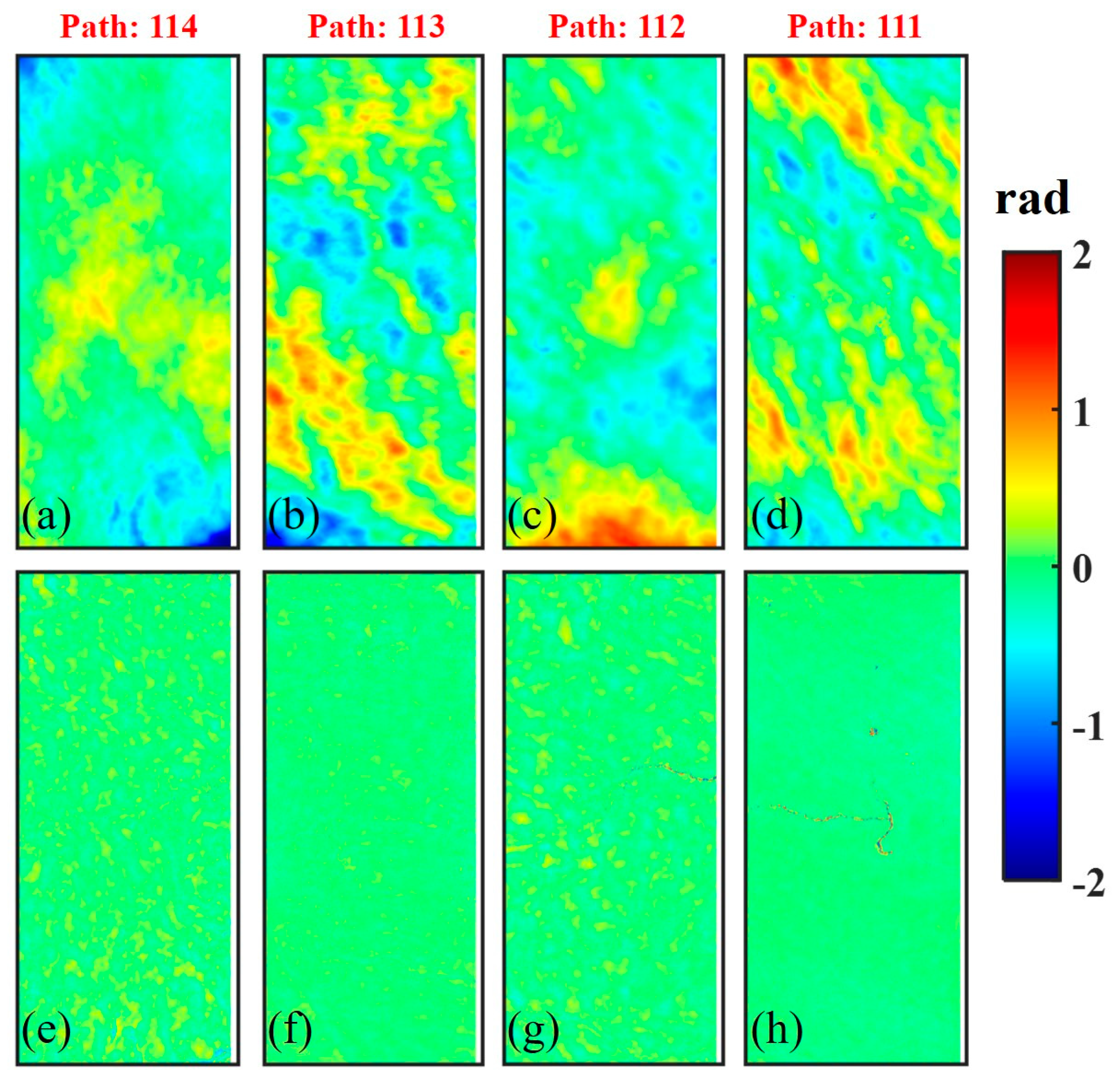
4.1. Inland Test Site

Aiming to construct an observation equation for block adjustment that considers both systematic errors and atmospheric delay errors, the reliability of GCPs and TPs is essential. Figure 4 shows the distribution of GCPs and TPs in the inland test site, where Figure 4a represents the control point database established using the selection rules in Table 1, and Figure 4b displays the GCPs and TPs after refinement and thinning. The uniform distribution provides support for systematic error calibration.

The existing research indicated that atmospheric delay errors mainly include tropospheric delay errors and ionospheric delay errors [26]. Since the ionospheric delay error is a long-wavelength signal usually manifested as the orbit error, it will cause the scene-by-scene polynomial fitting method to correct the orbit error phase to fail [29]. To overcome the influence of trend errors of ionospheric delay errors on polynomial fitting orbit error, we used the coarse block adjustment to provide the SA-MRWCA with more accurate orbit error phases for correcting atmospheric effects. Sub-aperture decomposition was employed to form F-Infs and B-Infs. Then, we utilized SRTM DEM and ASTER GDEM to perform differential interferometry, respectively. Subsequently, the orbit error phase of F-DInf and B-DInf was removed to guarantee the ADP’s unique similarity. Figure 5 compares the above two methods for removing the orbit error phase, where Figure 5a–d shows scene-by-scene polynomial fitting, and Figure 5e–h displays coarse block adjustment estimates.

Apparent trend errors are observed at the top of Figure 5b–d but are weakened in Figure 5f–h. In the orange frame of Figure 5, Figure 5f shows an ionospheric delay phase similar to the orbit error phase. We can find that the scene-by-scene polynomial fitting orbit error phase was interfered with by the ionospheric delay phase and absorbed part of it, resulting in a residual orbit error signal at the top of Figure 5b. In addition, comparing the black frame and red frame in Figure 5, it can be seen that the trend errors in Figure 5c are weakened in Figure 5g. The above differences prove that benefiting from the elevation control of GCPs and the elevation consistency constraint of TPs, the systematic errors estimated by coarse block adjustment can overcome the interference of atmospheric delay errors to a certain extent and better separate the two. As a result, this provides the basis for the SA-MRWCA to correct atmospheric effects. The remaining phase components after removing the orbit error phase are shown in Equation (11).

Since the TEP comes from different DEMs and the NP is random, the ADP is the only similar phase component between F-DInfs and B-DInfs. In the frequency domain, the TEP and the NP are mainly composed of high-frequency signals, while the ADP mostly appears as low-frequency signals. The above phase components are mixed in the differential interferograms and are difficult to separate effectively through spatial domain filtering. However, the different signal characteristics provide the basis for detecting the ATP. Therefore, we proposed the SA-MRWCA method to decompose F-DInfs and B-DInfs into multiple phase signals of different wavelengths through forward wavelet transform. Then, the SA-MRWCA used weighted correlation analysis to reduce the TEP and NP signals, reconstructing the ADP through inverse wavelet transform. Figure 6a–h displays the detected ADP and the phase after atmospheric correction of the inland test site, respectively. Combining with Figure 5e–h, we find that the SA-MRWCA correctly detected atmospheric delay errors.

After obtaining the atmospheric delay errors, the error equations considering the atmospheric delay errors can be established, achieving height matching between DEMs and GCPs, as well as between TPs. In addition, to construct a more stable block adjustment solution method in fine block adjustment, we utilized the t-test to test the significance of model parameters and realized the adaptation of systematic errors. On this basis, since GCPs and TPs came from two types of observation systems, and the error equations were affected by gross errors, the RHVCE [22] was to establish an accurate posterior stochastic model for calculating the parameters. Finally, we used the error correction equation shown in Equation (14) to correct the InSAR-DEM in the inland test site.

The results and accuracy statistics are shown in Figure 7, where Figure 7a displays the corrected DEM, and Figure 7b shows the error statistics histogram of the DEMs corrected by block adjustment considering and ignoring atmospheric effects compared with ICESat-2 elevation validation points. The block adjustment considering atmospheric effects markedly enhanced error concentration, reducing the root mean square error (RMSE) from 10.85 m to 3.02 m and resulting in a 72.2% increase in height accuracy. In order to spatially evaluate whether systematic errors and atmospheric delay errors have been removed, we introduced TanDEM-X DEM as elevation reference data and conducted a local comparison at the red frame in Figure 7a. Figure 7c partially enlarges the view of the corrected DEM. The difference map between the InSAR-DEM of the area and TanDEM-X DEM under block adjustment considering and ignoring atmospheric effects is shown in Figure 7d,e, respectively. The red frame contains three strips. Figure 7d displays calibration considering atmospheric effects, which removes the atmospheric delay errors and systematic errors completely. However, Figure 7e exhibits significant residual error trends, indicating that block adjustment ignoring atmospheric effects cannot accurately estimate the systematic errors of each strip.

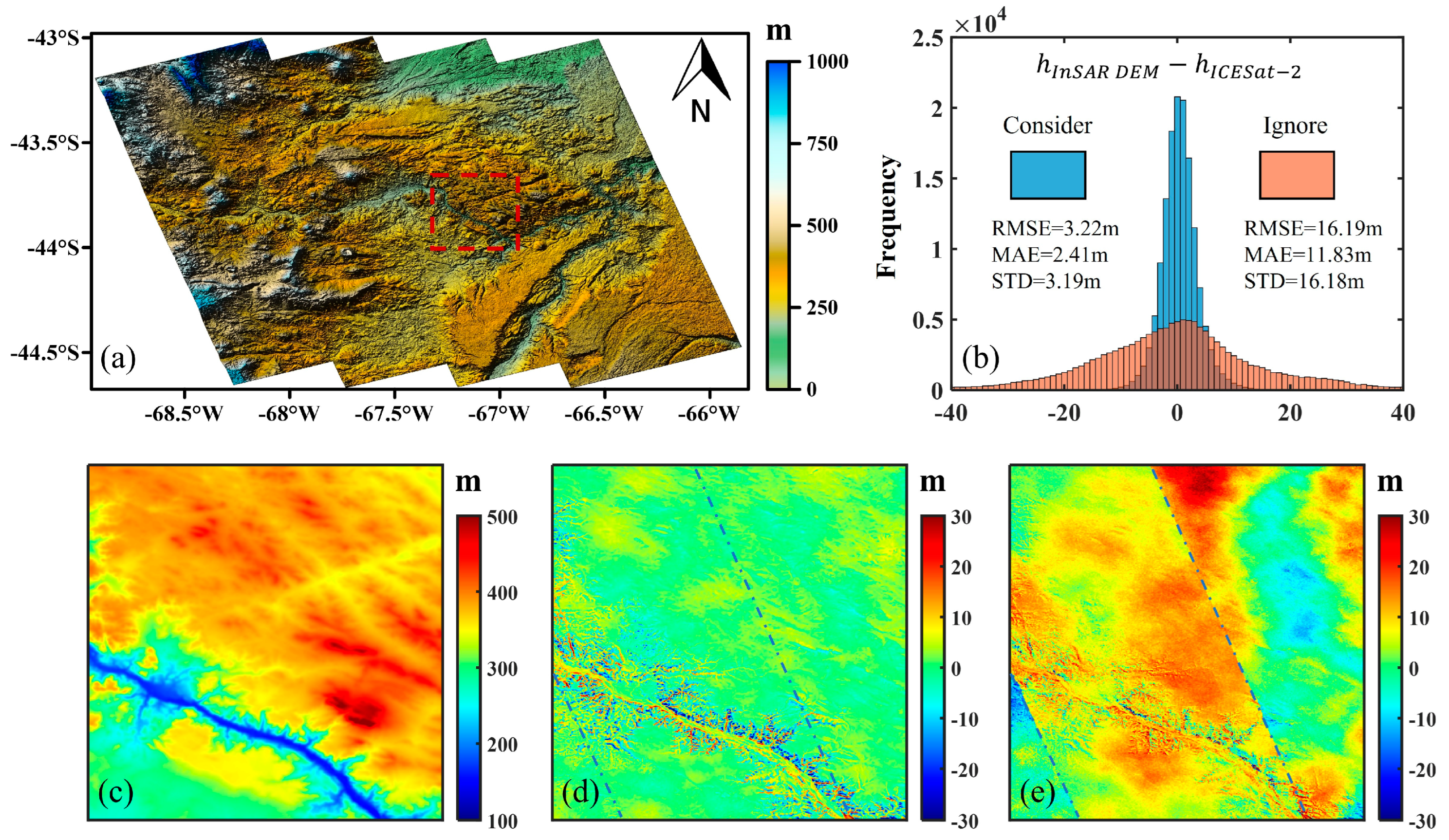
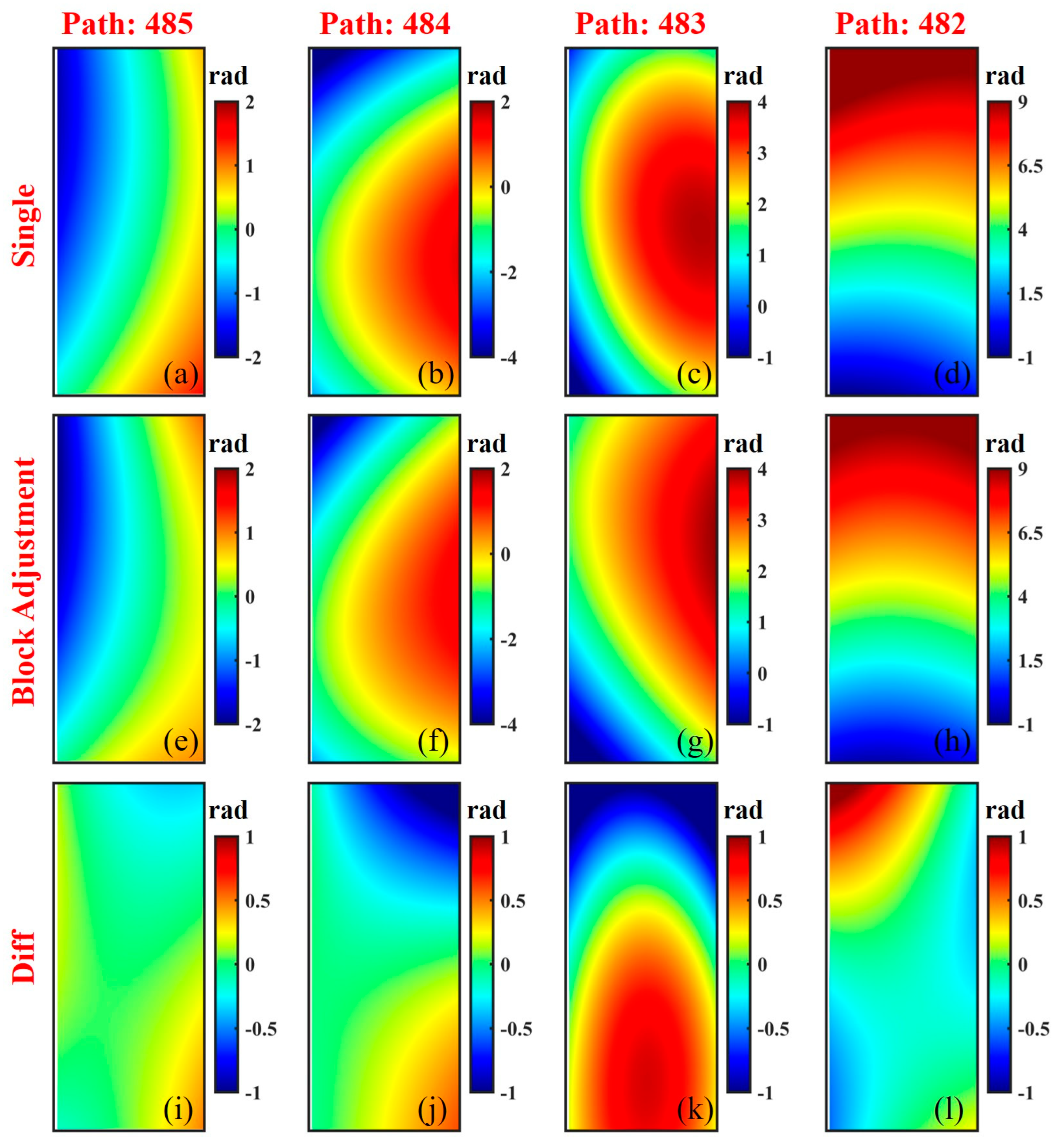
4.2. Coastal Test Site

The coastal test site lies east of the Atlantic Ocean, characterized by scattered hills with elevations ranging from approximately 100 to 750 m. Compared with the inland test site, the coastal test site has a more humid atmospheric layer and a more undulating terrain. Additionally, as shown in Table 2, the vertical baselines in the inland test site are concentrated between 300 and 550 m. In contrast, the coastal test site exhibits significant differences in vertical baselines between adjacent strips, with variations exceeding 300 m, implying that each strip has different sensitivities to the ADP and the TEP. Therefore, the coastal test site has more difficulty detecting atmospheric delay errors and estimating systematic errors using the proposed algorithm. The distribution of GCPs and TPs in the coastal test site is shown in Figure 8, where Figure 8a represents the control point database, and Figure 8b represents the GCPs and TPs after refinement and thinning.

After making the ADP the only similar phase component between F-DInfs and B-DInfs, we can detect the ADP based on the SA-MRWCA and correct the atmospheric delay errors, shown in Figure 9a–h, respectively. Previous studies have indicated that the tropospheric delay errors, as one of the main components of atmospheric effects, can be divided into topography-dependent vertical stratified delay and topography-independent turbulent delay [26]. When comparing Figure 6a–d with Figure 9a–d, it is evident that the ADP extracted in the coastal test site appears relatively discrete. This discreteness can be attributed to the dispersed hills in the coastal test site, where the topography undergoes rapid changes, resulting in the incorporation of topography-dependent signals in the atmospheric delay. In addition, considering that the ground surface will not deform in a short period, the positive phase at the bottom of Figure 9c should be topography-independent turbulence signals. After atmospheric correction, the residual phases shown in Figure 9e–h have no apparent atmospheric delay signals. Due to the relatively shorter vertical baselines of Path 111 and Path 113, the height of ambiguity (height change corresponding to one phase cycle) is 500 m and 410 m, respectively, leading to smaller TEP values, as depicted in Figure 9f,h. Height matching was achieved between DEMs and GCPs, as well as between TPs, through the atmospheric delay error estimated by the SA-MRWCA. On this basis, we utilized RHVCE in fine block adjustment to establish an accurate posterior stochastic model for resisting the influence of gross errors on the observation equations. Finally, we calculated the model parameters to correct the InSAR-DEM in the coastal test site.

Figure 10 shows the results and the height accuracy statistics, where Figure 10a displays the corrected DEM, and Figure 10b displays the error statistics histogram of the DEMs corrected by block adjustment considering and ignoring atmospheric effects compared with ICESat-2 elevation validation points. It can be seen that the errors after correction of the block adjustment considering atmospheric effects are more concentrated, the RMSE reduced from 16.19 m to 3.22 m, and the height accuracy increased by 80.2%. In addition, we also introduced TanDEM-X DEM to test the calibration effect and conducted a local comparison in the red frame in Figure 10a. Figure 10c is a partially enlarged view of the corrected DEM. The difference map between the InSAR-DEM of the area and TanDEM-X DEM under the block adjustment considering and ignoring the atmospheric effects is shown in Figure 10d,e. The red frame contains three strips. When comparing Figure 10d with Figure 10e, it can be seen that the block adjustment considering atmospheric effects completely corrected systematic errors and atmospheric delay errors. However, the block adjustment ignoring atmospheric effects shows apparent elevation discontinuities in the overlapping area, indicating a misestimation of systematic errors. The correction results in the coastal test area illustrate that our algorithm is still effective when the water vapor content is rich and the baselines between adjacent strips differ.

5. Discussion

5.1. The Impact of Atmospheric Effects on the Estimation of Block Adjustment

Through the above analysis, we can find that the impact of atmospheric effects on block adjustment mainly includes two aspects.

(1)

Height matching between InSAR-DEM and GCPs, as well as between TPs

DLR proposed the block adjustment based on the function model, aiming to calibrate the systematic errors of the bistatic mode [9,10]. Therefore, the error equations of this model only observe systematic errors. In the repeat-pass interferometric mode, changes in the state of the atmosphere lead to the introduction of atmospheric delay errors in the DEM. When the relative humidity of the atmosphere changes by 20%, the resulting height measurement deviation can reach 80~290 m [26]. In addition to systematic errors, the height differences between DEMs and GCPs, as well as between TPs, also include atmospheric delay errors. In order to achieve height matching, it is crucial to establish an error equation that considers systematic errors and atmospheric delay errors. As shown in Figure 7e and Figure 10e, without considering the atmospheric effects, the estimated model parameters through block adjustment are inaccurate, resulting in residual trend signals in DEM. In contrast, Figure 7d and Figure 10d depict the difference maps between the DEMs corrected by our algorithm and TanDEM-X DEM, which observe no residual trend errors. It demonstrates the effectiveness of our algorithm in overcoming the atmospheric effects on height matching and accurately rectifying systematic errors.

(2)

The long-wavelength signals of atmospheric effects are mixed with systematic errors

Since the trajectory of SAR satellites in space is relatively smooth, systematic errors caused by inaccurate orbit positions usually exist in the form of long-wavelength signals [28]. However, the ionospheric delay errors of the atmospheric effects are also long-wavelength signals, which have a similar distribution to the systematic errors [29]. Therefore, it will interfere with the estimating of systematic errors. However, combined with the height control of GCPs and the height consistency constraint of TPs, block adjustment is more resistant to the interference of atmospheric delay errors than scene-by-scene polynomial fitting.

Systematic errors exist as the orbit error phase at the interferometric phase. As shown in Figure 5b,f, the ionospheric delay phase in the red frame is absorbed by the polynomial of the fitted orbit error phase when correcting the systematic error scene by scene, causing an underestimation of the top system error. When the orbit error phase is removed using the systematic error estimated by the block adjustment, the ionospheric delay phase appears in the remaining phase component, indicating that the two are well separated. Taking the inland test site as an example, the systematic errors estimated by scene-by-scene fitting and block adjustment are shown in Figure 11a–h, respectively. Due to the limited orbit position accuracy, the systematic error trends shown in Figure 11 are relatively changeable. Benefiting from the significance test based on the t-test, the systematic error estimation of block adjustment can achieve adaptive estimation for each strip. The systematic errors estimated by the above methods are pretty different. Figure 11i–l displays the difference maps between the two. Due to the interference of atmospheric delay errors, the systematic error estimated scene by scene in Figure 11c shows local overfitting. Combining Figure 5c,g and Figure 11g, it can be seen that the block adjustment overcomes the problem of local overfitting. The above analysis demonstrates that the block adjustment considering atmospheric effects can still estimate the complex systematic errors under the interference of atmospheric delay errors.

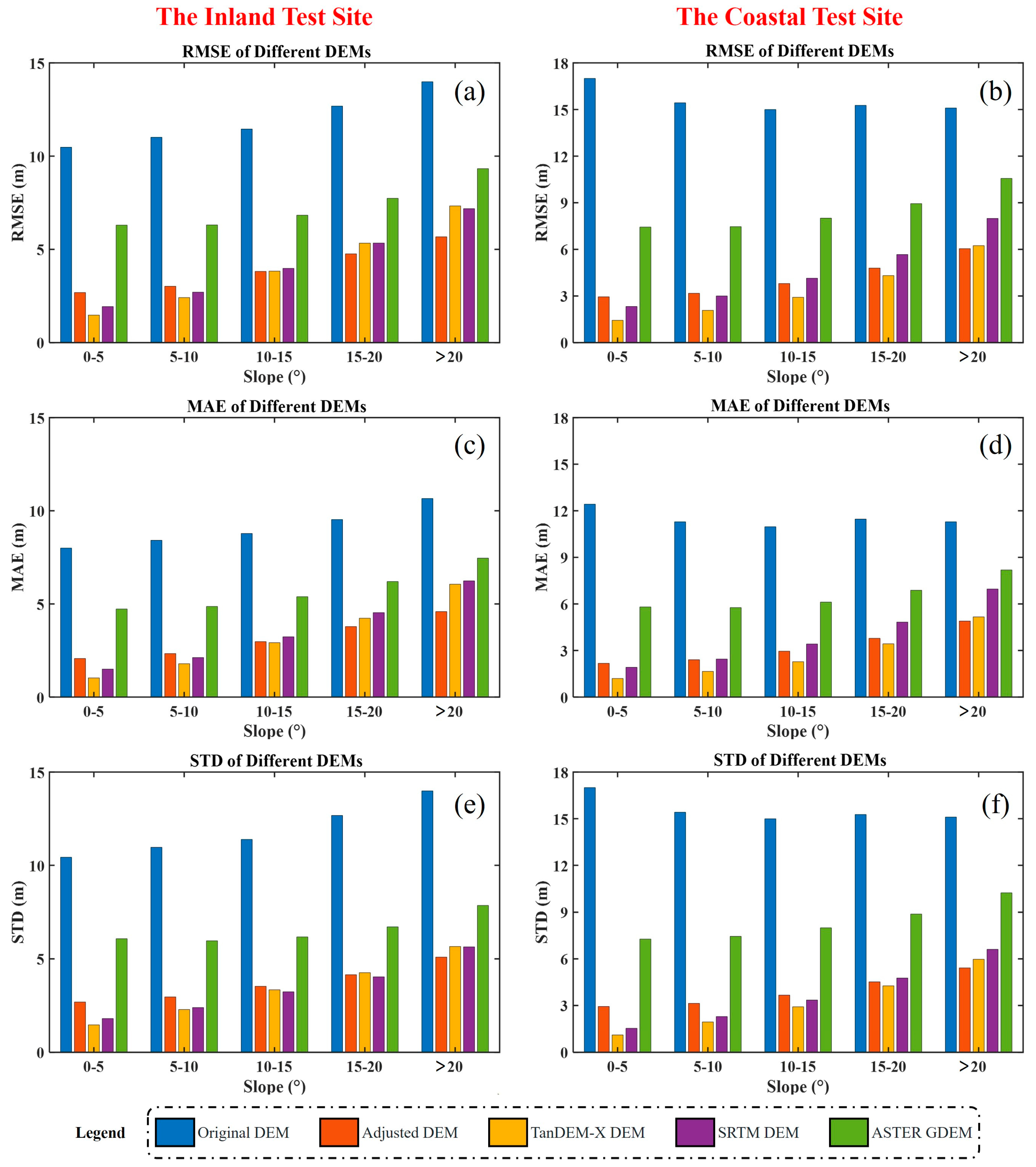
5.2. The Impact of Slope on DEM Calibration

In the block adjustment model considering atmospheric effects, the slope is another influencing factor besides atmospheric effects. Since the SAR uses side-looking imaging, geometric distortion can occur in steep slopes, resulting in limited DEM accuracy [26]. In addition, areas with large slopes often include mountains and hills, which are likely to contain topography-dependent tropospheric delay errors [26]. Based on the above factors, we divided the established control point database into five groups according to slope and then conducted height accuracy verification. The grouping situation is shown in

Table 4. The count of checkpoints in each category after being grouped by the slope.

Test Sites	0~5°	5~10°	10~15°	15~20°	>20°
Inland	151,680	102,129	27,047	6448	2403
Coastal	71,292	50,441	15,840	3641	1064

.

We used the grouped checkpoints to assess InSAR-DEMs’ accuracy in the inland and coastal test sites and then compared them with TanDEM-X DEM, SRTM DEM, and ASTER GDEM, respectively. The results are shown in Figure 12, where Figure 12a,c,e and Figure 12b,d,f are the RMSE, mean absolute error (MAE), and standard deviation (STD) of the inland and coastal test sites, respectively. With increasing slopes, the RMSE, MAE, and STD of the above DEMs decrease. However, compared with the original DEM, the accuracy indicators of the corrected DEM are significantly improved at each slope. In addition, the accuracy indicators of the corrected DEM are closer to TanDEM-X DEM and SRTM DEM produced by the zero-time baseline, which can prove the reliability of our algorithm in calibrating atmospheric delay errors and systematic errors.

6. Conclusions

Aiming at the block adjustment being interfered with by atmospheric effects for the BIOMASS mission, we proposed a block adjustment model considering atmospheric effects. This method separated systematic errors and atmospheric delay errors and then utilized the SA-MRWCA to detect atmospheric effects without relying on external water vapor data. Subsequently, the error equations containing the systematic errors and atmospheric delay errors can be established, achieving height matching between GCPs and DEMs, as well as between TPs. Finally, we used a significance test based on the t-test to achieve adaptive systematic error correction. Building on this foundation, we assessed the weights of GCPs and TPs by using the stochastic model estimated by RHVCE and then estimated the model parameters of block adjustment. Therefore, the atmospheric delay errors and systematic errors can be calibrated simultaneously, achieving block adjustment that overcomes the influence of atmospheric effects.

Through experiments with different climate conditions, we substantiated the algorithm’s effectiveness. Furthermore, a precision comparison was conducted between the original DEM, corrected DEM, and global DEM products at varying slopes. Compared with the original DEM, the height accuracy of the corrected DEM is closer to TanDEM-X DEM and SRTM DEM at each slope, indicating the algorithm can simultaneously correct atmospheric delay errors and systematic errors. In addition, the computational complexity and processing time depend on the quality of the satellite orbit, the reliability of the GCPs and TPs, and the distribution of systematic errors and atmospheric delay errors.

Since there are no available spaceborne P-band data, L-band data are the best means of simulation. The P-band has a longer wavelength than the L-band, which will cause it to experience more severe ionospheric delay errors. Furthermore, the P-band and L-band have different penetration capabilities into the forests, resulting in different forest responses to SAR signals. Therefore, future research should validate the proposed model using the actual BIOMASS data. What is particularly important is that to avoid forest signal interference with systematic error observations, existing studies mainly select the GCPs and TPs on bare earth. However, the core monitoring object of BIOMASS is the forest. An even distribution of the GCPs and TPs is necessary to ensure accurate observation of systematic errors. Therefore, it is urgent to establish a P-band scattering model that considers differences in penetration depths to forests and then overcomes their impact on DEM calibration.

References

1. Rizzoli, P.; Martone, M.; Gonzalez, C.; Wecklich, C.; Borla Tridon, D.; Bräutigam, B.; Bachmann, M.; Schulze, D.; Fritz, T.; Huber, M.; et al. Generation and Performance Assessment of the Global TanDEM-X Digital Elevation Model. ISPRS J. Photogramm. Remote Sens. 2017, 132, 119–139. [Google Scholar] [CrossRef]
2. Rodriguez, E.; Morris, C.; Belz, J.; Chapin, E.; Martin, J.; Daffer, W.; Hensley, S. An Assessment of the SRTM Topographic Products. 2005. Available online: https://www.researchgate.net/publication/235704654_An_assessment_of_the_SRTM_topographic_products_Technical_Report_JPL_D-31639 (accessed on 12 May 2024).
3. Le Toan, T.; Quegan, S.; Davidson, M.W.J.; Balzter, H.; Paillou, P.; Papathanassiou, K.; Plummer, S.; Rocca, F.; Saatchi, S.; Shugart, H.; et al. The BIOMASS Mission: Mapping Global Forest Biomass to Better Understand the Terrestrial Carbon Cycle. Remote Sens. Environ. 2011, 115, 2850–2860. [Google Scholar] [CrossRef]
4. Fatoyinbo, T.; Armston, J.; Simard, M.; Saatchi, S.; Denbina, M.; Lavalle, M.; Hofton, M.; Tang, H.; Marselis, S.; Pinto, N.; et al. The NASA AfriSAR Campaign: Airborne SAR and Lidar Measurements of Tropical Forest Structure and Biomass in Support of Current and Future Space Missions. Remote Sens. Environ. 2021, 264, 112533. [Google Scholar] [CrossRef]
5. Quegan, S.; Chave, J.; Dall, J.; Le Toan, T.; Papathanassiou, K.; Rocca, F.; Saatchi, S.; Scipal, K.; Shugart, H.; Ulander, L.; et al. The Science and Measurement Concepts Underlying the BIOMASS Mission. In Proceedings of the 2012 IEEE International Geoscience and Remote Sensing Symposium, Munich, Germany, 22–27 July 2012; pp. 5542–5545. [Google Scholar]
6. Banda, F.; Giudici, D.; Le Toan, T.; d’Alessandro, M.M.; Papathanassiou, K.; Quegan, S.; Riembauer, G.; Scipal, K.; Soja, M.; Tebaldini, S.; et al. The BIOMASS Level 2 Prototype Processor: Design and Experimental Results of Above-Ground Biomass Estimation. Remote Sens. 2020, 12, 985. [Google Scholar] [CrossRef]
7. Quegan, S.; Lomas, M.; Papathanassiou, K.P.; Kim, J.-S.; Tebaldini, S.; Giudici, D.; Scagliola, M.; Guccione, P.; Dall, J.; Dubois-Fenandez, P.; et al. Calibration Challenges for the Biomass P-Band SAR Instrument. In Proceedings of the IGARSS 2018—2018 IEEE International Geoscience and Remote Sensing Symposium, Valencia, Spain, 22–27 July 2018; pp. 8575–8578. [Google Scholar]
8. Ferretti, A.; Prati, C.; Rocca, F. Permanent Scatterers in SAR Interferometry. IEEE Trans. Geosci. Remote Sens. 2001, 39, 8–20. [Google Scholar] [CrossRef]
9. Wessel, B.; Gruber, A.; Huber, M.; Roth, A. TanDEM-X: Block Adjustment of Interferometric Height Models. In Proceedings of the ISPRS Hannover Workshop 2009 “High-Resolution Earth Imaging for Geospatioal Information”, International Archives of the Photogrammetry, Remote Sensing and Spatial Information Sciences, Hannover, Germany, 2–5 June 2009; pp. 1–6. Available online: https://elib.dlr.de/62358/ (accessed on 12 May 2024).
10. Wessel, B.; Gruber, A.; Gonzalez, J.H.; Bachmann, M.; Wendleder, A. TanDEM-X: DEM Calibration Concept. In Proceedings of the IGARSS 2008—2008 IEEE International Geoscience and Remote Sensing Symposium, Boston, MA, USA, 7–11 July 2008; Volume 3, pp. III-111–III-114. [Google Scholar]
11. Gruber, A.; Wessel, B.; Huber, M.; Roth, A. Operational TanDEM-X DEM Calibration and First Validation Results. ISPRS J. Photogramm. Remote Sens. 2012, 73, 39–49. [Google Scholar] [CrossRef]
12. Schutz, B.E.; Zwally, H.J.; Shuman, C.A.; Hancock, D.; DiMarzio, J.P. Overview of the ICESat Mission. Geophys. Res. Lett. 2005, 32, 2005GL024009. [Google Scholar] [CrossRef]
13. Markus, T.; Neumann, T.; Martino, A.; Abdalati, W.; Brunt, K.; Csatho, B.; Farrell, S.; Fricker, H.; Gardner, A.; Harding, D.; et al. The Ice, Cloud, and Land Elevation Satellite-2 (ICESat-2): Science Requirements, Concept, and Implementation. Remote Sens. Environ. 2017, 190, 260–273. [Google Scholar] [CrossRef]
14. Huber, M.; Wessel, B.; Kosmann, D.; Felbier, A.; Schwieger, V.; Habermeyer, M.; Wendleder, A.; Roth, A. Ensuring Globally the TanDEM-X Height Accuracy: Analysis of the Reference Data Sets ICESat, SRTM and KGPS-Tracks. In Proceedings of the 2009 IEEE International Geoscience and Remote Sensing Symposium, Cape Town, South Africa, 12–17 July 2009; IEEE: Piscataway, NJ, USA, 2009; pp. II-769–II-772. [Google Scholar]
15. Hueso Gonzalez, J.; Bachmann, M.; Scheiber, R.; Krieger, G. Definition of ICESat Selection Criteria for Their Use as Height References for TanDEM-X. IEEE Trans. Geosci. Remote Sens. 2010, 48, 2750–2757. [Google Scholar] [CrossRef]
16. Wang, R.; Lv, X.; Zhang, L. A Novel Three-Dimensional Block Adjustment Method for Spaceborne InSAR-DEM Based on General Models. IEEE J. Sel. Top. Appl. Earth Obs. Remote Sens. 2023, 16, 3973–3987. [Google Scholar] [CrossRef]
17. Wang, R.; Lv, X.; Chai, H.; Zhang, L. A Three-Dimensional Block Adjustment Method for Spaceborne InSAR Based on the Range-Doppler-Phase Model. Remote Sens. 2023, 15, 1046. [Google Scholar] [CrossRef]
18. Huber, S.; de Almeida, F.Q.; Villano, M.; Younis, M.; Krieger, G.; Moreira, A. Tandem-L: A Technical Perspective on Future Spaceborne SAR Sensors for Earth Observation. IEEE Trans. Geosci. Remote Sens. 2018, 56, 4792–4807. [Google Scholar] [CrossRef]
19. Xiao, R.; Yu, C.; Li, Z.; He, X. Statistical Assessment Metrics for InSAR Atmospheric Correction: Applications to Generic Atmospheric Correction Online Service for InSAR (GACOS) in Eastern China. Int. J. Appl. Earth Obs. Geoinf. 2021, 96, 102289. [Google Scholar] [CrossRef]
20. Dou, F.; Lv, X.; Chai, H. Mitigating Atmospheric Effects in InSAR Stacking Based on Ensemble Forecasting with a Numerical Weather Prediction Model. Remote Sens. 2021, 13, 4670. [Google Scholar] [CrossRef]
21. Jung, H.-S.; Won, J.-S.; Kim, S.-W. An Improvement of the Performance of Multiple-Aperture SAR Interferometry (MAI). IEEE Trans. Geosci. Remote Sens. 2009, 47, 2859–2869. [Google Scholar] [CrossRef]
22. Yang, Y.; Xu, T.; Song, L. Robust Estimation of Variance Components with Application in Global Positioning System Network Adjustment. J. Surv. Eng. 2005, 131, 107–112. [Google Scholar] [CrossRef]
23. Gonzalez, J.H.; Bachmann, M.; Krieger, G.; Fiedler, H. Development of the TanDEM-X Calibration Concept: Analysis of Systematic Errors. IEEE Trans. Geosci. Remote Sens. 2010, 48, 716–726. [Google Scholar] [CrossRef]
24. Liu, Z.; Fu, H.; Zhu, J.; Zhou, C.; Zuo, T. Using Dual-Polarization Interferograms to Correct Atmospheric Effects for InSAR Topographic Mapping. Remote Sens. 2018, 10, 1310. [Google Scholar] [CrossRef]
25. Fu, H.Q.; Zhu, J.J.; Wang, C.C.; Zhao, R.; Xie, Q.H. Atmospheric Effect Correction for InSAR With Wavelet Decomposition-Based Correlation Analysis Between Multipolarization Interferograms. IEEE Trans. Geosci. Remote Sens. 2018, 56, 5614–5625. [Google Scholar] [CrossRef]
26. Hanssen, R.F. Radar Interferometry: Data Interpretation and Error Analysis; Kluwer: Norwell, MA, USA, 2001. [Google Scholar]
27. Abrams, M.; Crippen, R.; Fujisada, H. ASTER Global Digital Elevation Model (GDEM) and ASTER Global Water Body Dataset (ASTWBD). Remote Sens. 2020, 12, 1156. [Google Scholar] [CrossRef]
28. Shirzaei, M.; Walter, T.R. Estimating the Effect of Satellite Orbital Error Using Wavelet-Based Robust Regression Applied to InSAR Deformation Data. IEEE Trans. Geosci. Remote Sens. 2011, 49, 4600–4605. [Google Scholar] [CrossRef]
29. Liao, H.; Meyer, F.J.; Scheuchl, B.; Mouginot, J.; Joughin, I.; Rignot, E. Ionospheric Correction of InSAR Data for Accurate Ice Velocity Measurement at Polar Regions. Remote Sens. Environ. 2018, 209, 166–180. [Google Scholar] [CrossRef]
30. Rosenqvist, A.; Shimada, M.; Ito, N.; Watanabe, M. ALOS PALSAR: A Pathfinder Mission for Global-Scale Monitoring of the Environment. IEEE Trans. Geosci. Remote Sens. 2007, 45, 3307–3316. [Google Scholar] [CrossRef]
31. Li, Y.; Fu, H.; Zhu, J.; Wu, K.; Yang, P.; Wang, L.; Gao, S. A Method for SRTM DEM Elevation Error Correction in Forested Areas Using ICESat-2 Data and Vegetation Classification Data. Remote Sens. 2022, 14, 3380. [Google Scholar] [CrossRef]
32. Neuenschwander, A.; Guenther, E.; White, J.C.; Duncanson, L.; Montesano, P. Validation of ICESat-2 Terrain and Canopy Heights in Boreal Forests. Remote Sens. Environ. 2020, 251, 112110. [Google Scholar] [CrossRef]
Figure 1. Flow chart of InSAR-DEM block adjustment considering atmospheric effects.
Remotesensing 16 01764 g001
Figure 2. The location and the ALOS-1 footprint of the inland test site. The numbers are the index of the SAR data.
Remotesensing 16 01764 g002
Figure 3. The location and the ALOS-1 footprint of the coastal test site. The numbers are the index of the SAR data.
Remotesensing 16 01764 g003
Figure 4. (a) The control point database of the inland test site; (b) the distribution of GCPs and TPs in the inland test site.
Remotesensing 16 01764 g004
Figure 5. Comparison of different methods for removing orbit error phase in inland test site: (ad) scene-by-scene polynomial fitting; (eh) block adjustment estimates. The boxes show the difference.
Remotesensing 16 01764 g005
Figure 6. The atmospheric correction results of the inland test site: (ad) ATP estimated by the SA-MRWCA; (eh) residual phase after atmospheric correction.
Remotesensing 16 01764 g006
Figure 7. DEM calibration results and accuracy verification in the inland test site: (a) corrected DEM; (b) error statistical histogram of the corrected DEMs by block adjustment considering and neglecting atmospheric effects. (ce) are partially enlarged views of the red frame in (a): (c) partial map of the corrected DEM; (d) difference map between (c) and TanDEM-X DEM; (e) difference map between the partial DEM ignoring atmospheric effects and TanDEM-X DEM.
Remotesensing 16 01764 g007
Figure 8. (a) The control point database of the coastal test site; (b) the distribution of GCPs and TPs in the coastal test site.
Remotesensing 16 01764 g008
Figure 9. The atmospheric correction results of the coastal test site: (ad) ATP estimated by the SA-MRWCA; (eh) residual phase after atmospheric correction.
Remotesensing 16 01764 g009
Figure 10. DEM calibration results and accuracy verification in the coastal test site: (a) corrected DEM; (b) error statistical histogram of the corrected DEMs by block adjustment considering and neglecting atmospheric effects. (ce) are partially enlarged views of the red frame in (a): (c) partial map of the corrected DEM; (d) difference map between (c) and TanDEM-X DEM; (e) difference map between the partial DEM ignoring atmospheric effects and TanDEM-X DEM.
Remotesensing 16 01764 g010
Figure 11. Comparison of systematic errors between scene-by-scene fitting and block adjustment fitting in the inland test site: (ad) scene-by-scene fitting; (eh) block adjustment fitting; (il) difference maps in estimated systematic errors between scene-by-scene fitting and block adjustment fitting.
Remotesensing 16 01764 g011
Figure 12. Comparison between the original DEM, corrected DEM, TanDEM-X DEM, SRTM DEM, and ASTER GDEM at varying slopes: (a,c,e) the RMSE, MAE, and STD of different DEMs in inland test site; (b,d,f) the RMSE, MAE, and STD of different DEMs in coastal test site.
Remotesensing 16 01764 g012